Antipode Preserving Cubic Maps:
the Fjord Theorem

Abstract.

This note will study a family of cubic rational maps which carry antipodal points of the Riemann sphere to antipodal points. We focus particularly on the fjords, which are part of the central hyperbolic component but stretch out to infinity. These serve to decompose the parameter plane into subsets, each of which is characterized by a corresponding rotation number.

1. Introduction.

By a classical theorem of Borsuk (see [Bo]):

There exists a degree $d$ map from the $n$-sphere to itself carrying antipodal points to antipodal points if and only if $d$ is odd.

For the Riemann sphere, ${\widehat{\mathbb{C}}}={\mathbb{C}}\cup\{\infty\}\cong~{}S^{2}$, the antipodal map is defined to be the fixed point free map ${\mathpzc A}(z)=-1/\overline{z}$. We are interested in rational maps from the Riemann sphere to itself which carry antipodal points to antipodal points, so that ${\mathpzc A}\circ f=f\circ{\mathpzc A}$. If all of the zeros $q_{j}$ of $f$ lie in the finite plane, then $f$ can be written uniquely as

$$f(z)=u\prod_{j=1}^{d}\frac{z-q_{j}}{1+\overline{q}_{j}z}\qquad{\rm with}\qquad|u|=1.$$

The simplest interesting case is in degree $d=3$. To fix ideas we will discuss only the special case where $f$ has a critical fixed point. Putting this fixed point at the origin, we can take $q_{1}=q_{2}=0$, and write $q_{3}$ briefly as $q$. It will be convenient to take $u=-1$, so that the map takes the form

$$f(z)=f_{q}(z)=z^{2}\frac{q-z}{1+\overline{q}z}.$$ (1)

(Note that there is no loss of generality in choosing one particular value for $u$, since we can always change to any other value of $u$ by rotating the $z$-plane appropriately.)

Figure 1. The $q$-parameter plane.

Figure 1 illustrates the $q$-parameter plane for this family of maps: (1).

$\bullet$ The central white region, resembling a porcupine, is the hyperbolic component centered at the map $f_{0}(z)=-z^{3}$. It consists of all $q$ for which the Julia set is a Jordan curve separating the basins of zero and infinity. This region is simply-connected (see Lemma 3.1); but its boundary is very far from locally connected. (See [BBM2], the sequel to this paper.)

$\bullet$ The colored regions in Figure 1 will be called tongues, in analogy with Arnold tongues. Each of these is a hyperbolic component, stretching out to infinity. Each representative map $f_{q}$ for such a tongue has a self-antipodal cycle of attracting basins which are arranged in a loop separating zero from infinity. (Compare Figure 2.) Each such loop has a well defined combinatorial rotation number, as seen from the origin, necessarily rational with even denominator. These rotation numbers are indicated in Figure 1 by colors which range from red (for rotation number close to zero) to blue (for rotation number close to one).

Figure 2. Rational rotation number with even denominator: Julia set for a point in the $(21/26)$-tongue. Here the Riemann sphere has been projected orthonormally onto the plane, so that only one hemisphere is visible. Zero is at the bottom and infinity at the top. Note the self-antipodal attracting orbit of period $26$, which has been marked. The associated ring of attracting Fatou components separates the basins of zero and infinity. $($If the sphere were transparent, then we would see the same figure on the far side, but rotated $180^{\circ}$ and with light and dark gray interchanged.$)$

  

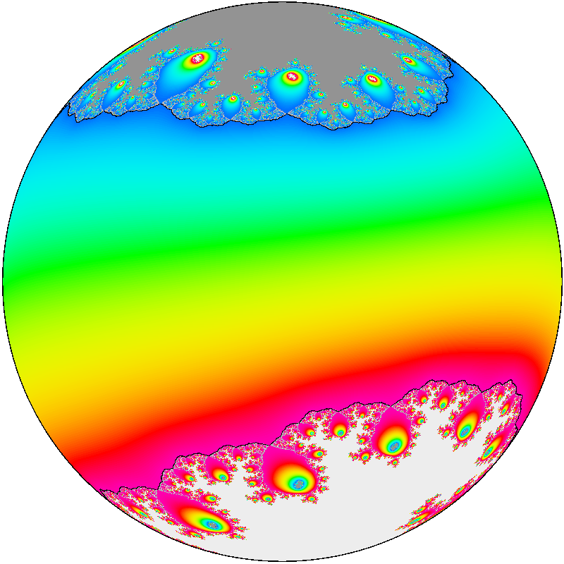
Figure 3. Irrational rotation number: two Herman rings on the Riemann sphere, projected orthonormally. The boundaries of the rings have been outlined. Otherwise, every point $z$ maps to a point $f_{q}(z)$ of the same color. Left example: $q=1-6i$, modulus $\approx 0.2081$. Right example: $q=3.21-1.8i$, modulus $\approx 0.0063$.

$\bullet$ The black region in Figure 1 is the Herman ring locus. For the overwhelming majority of parameters $q$ in this region, the map $f_{q}$ has a Herman ring which separates the basins of zero and infinity. (Compare Figure 3.) Every such Herman ring has a well defined rotation number (again as seen from zero), which is always a Brjuno number. If we indicate these rotation numbers also by color, then there is a smooth gradation, so that the tongues no longer stand out. (Compare Figures 5 and 5.)

$\bullet$ For rotation numbers with odd denominator, there are no such tongues or rings. Instead there are channels leading out to infinity within the central hyperbolic component. (Compare Figures 1 and 6.) These will be called fjords, and will be a central topic of this paper.

$\bullet$ The gray regions and the nearby small white regions in Figure 1 represent capture components, such that both of the critical points in ${\mathbb{C}}{\smallsetminus}\{0\}$ have orbits which eventually land in the immediate basin of zero (for white) or infinity (for gray).

Note that Figure 1 is invariant under $180^{\circ}$ rotation. In fact each $f_{q}$ is linearly conjugate to $f_{-q}(z)=-f_{q}(-z)$. In order to eliminate this duplication, it is often convenient to use $q^{2}$ as parameter. The $q^{2}$-plane of Figure 5, could be referred to as the moduli space, since each $q^{2}\in{\mathbb{C}}$ corresponds to a unique holomorphic conjugacy class of mappings of the form (1) with a marked critical fixed point at the origin.

Figure 4. The $q^{2}$-plane. Here the colors code the rotation number, not distinguishing between tongues and Herman rings.

Figure 5. Image of the circled $q^{2}$-plane under a homeomorphism $\quad\raisebox{-1.49994pt}{\includegraphics[width=9.39545pt]{cc-crop.pdf}}\to\overline{\mathbb{D}}$ which shrinks the circled plane to the unit disk.

Definition 1.1.

It is often useful to add a circle of points at infinity to the complex plane. The circled complex plane

$$\raisebox{-1.49994pt}{\includegraphics[width=9.39545pt]{cc-crop.pdf}}={\mathbb{C}}\cup({\rm circle~{}at~{}infinity})$$

will mean the compactification of the complex plane which is obtained by adding one point at infinity, ${\boldsymbol{\infty}}_{\bf t}\in\partial\raisebox{-1.49994pt}{\includegraphics[width=9.39545pt]{cc-crop.pdf}}$, for each ${\bf t}\in{{\mathbb{R}}/{\mathbb{Z}}}$; where a sequence of points $w_{k}\in{\mathbb{C}}$ converges to ${\boldsymbol{\infty}}_{\bf t}$ if and only if $|w_{k}|\to\infty$ and $w_{k}/|w_{k}|\to e^{2\pi i{\bf t}}$. By definition, this circled plane is homeomorphic to the closed unit disk $\overline{\mathbb{D}}$ under a homeomorphism $\raisebox{-1.49994pt}{\includegraphics[width=9.39545pt]{cc-crop.pdf}}\stackrel{{\scriptstyle\cong}}{{\longrightarrow}}\overline{\mathbb{D}}$ of the form

$$w=re^{2\pi i{\bf t}}\mapsto\eta(r)e^{2\pi i{\bf t}}$$

where $\eta:[0,\infty]\to[0,1]$ is any convenient homeomorphism. (For example we could take

$$\eta(r)=r\Big{/}\sqrt{1+r^{2}}$$

but the precise choice of $\eta$ will not be important.)

In particular, it is useful to compactify the $q^{2}$-plane in this way; and for illustrative purposes, it is often helpful to show the image of the circled $q^{2}$-plane under such a homeomorphism, since we can then visualize the entire circled plane in one figure. (Compare Figures 5 and 5.) The circle at infinity for the $s$-plane has an important dynamic interpretation:

Lemma 1.2.

Suppose that $q^{2}$ converges to the point ${\boldsymbol{\infty}}_{\bf t}$ on the circle at infinity. Then for any $\varepsilon>0$ the associated maps $f_{\pm q}$ both converge uniformly to the rotation $z\mapsto e^{2\pi i{\bf t}}z$ throughout the annulus $\varepsilon\leq|z|\leq 1/\varepsilon$.

Therefore, most of the chaotic dynamics must be concentrated within the small disk $|z|<\varepsilon$ and its antipodal image. The proof is a straightforward exercise.∎

Outline of the Main Concepts and Results.

In Section 2 of the paper we discuss the various types of Fatou components for maps $f_{q}$ with $q\in{\mathbb{C}}$. In particular, we show that any Fatou component which eventually maps to a Herman ring is an annulus, but that all other Fatou components are simply-connected. (See Theorem 2.1.)

We give a rough classification of hyperbolic components (either in the $q$-plane or in the $q^{2}$-plane), noting that every hyperbolic component is simply-connected, with a unique critically finite “center” point. (See Lemma 2.4.)

In Section 3 we focus on the study of the central hyperbolic component ${\pazocal H}_{0}$ in the $q^{2}$ plane. We construct a canonical (but not conformal !) diffeomorphism between ${{\pazocal H}_{0}}$ and the open unit disk (Lemma 3.1). Using this, we can consider parameter rays ($=$ stretching rays), which correspond to radial lines in the unit disk, each with a specified angle ${\boldsymbol{\vartheta}}\in{{\mathbb{R}}/{\mathbb{Z}}}$. We prove that the following landing properties of the parameter rays ${\pazocal R}_{\boldsymbol{\vartheta}}$.

(Theorem 3.5.) If the angle ${\boldsymbol{\vartheta}}\in{\mathbb{Q}}/{\mathbb{Z}}$ is periodic under doubling, then the parameter ray ${\pazocal R}_{\boldsymbol{\vartheta}}$ either:

• lands at a parabolic point on the boundary $\partial{{\pazocal H}_{0}}$,

• accumulates on a curve of parabolic boundary points, or

• lands at a point ${\boldsymbol{\infty}}_{\bf t}$ on the circle at infinity, where ${\bf t}={\bf t}({\boldsymbol{\vartheta}})$ can be described as the rotation number of ${\boldsymbol{\vartheta}}$ under angle doubling. (Compare §4.)

The proof of this Theorem makes use of dynamic internal rays ${\mathscr{R}}_{q,\theta}$, which are contained within the immediate basin of zero ${\mathscr{B}}_{q}$ for the map $f_{q}$. These are defined using the Böttcher coordinate ${\mathfrak{b}}_{q}$, which is well defined throughout some neighborhood of zero in the $z$-plane whenever $q\neq 0$.

In Section 4 we study, for $q^{2}\in{{\pazocal H}_{0}}$, the set of landing points of dynamic internal rays ${\mathscr{R}}_{q,\theta}$. More precisely, if $q^{2}\in{\pazocal R}_{\boldsymbol{\vartheta}}$ with ${\boldsymbol{\vartheta}}\in{{\mathbb{R}}/{\mathbb{Z}}}$, then the dynamic internal ray ${\mathscr{R}}_{q,\theta}$ lands if and only if $\theta$ is not an iterated preimage of ${\boldsymbol{\vartheta}}$ under doubling. In addition, the Julia set ${\mathscr{J}}(f_{q})$ is a quasicircle and there is a homeomorphism ${\boldsymbol{\eta}}_{q}:{{\mathbb{R}}/{\mathbb{Z}}}\to{\mathscr{J}}(f_{q})$ conjugating the tripling map to $f_{q}$:

$${\boldsymbol{\eta}}_{q}(3x)=f_{q}\bigl{(}{\boldsymbol{\eta}}_{q}(x)\bigr{)}.$$

This conjugacy is uniquely defined up to orientation, and up to the involution $x\leftrightarrow x+1/2$ of the circle. We specify a choice and present an algorithm which, given ${\boldsymbol{\vartheta}}\in{{\mathbb{R}}/{\mathbb{Z}}}$ and an angle $\theta\in{{\mathbb{R}}/{\mathbb{Z}}}$ which is not an iterated preimage of ${\boldsymbol{\vartheta}}$ under doubling, returns the base three expansion of the angle $x\in{{\mathbb{R}}/{\mathbb{Z}}}$ such that ${\boldsymbol{\eta}}_{q}(x)$ is the landing point of ${\mathscr{R}}_{q,\theta}$.

In Section 5 we define the dynamic rotation number ${\bf t}$ of a map $f_{q}$ for $q^{2}\in{{\pazocal H}_{0}}{\smallsetminus}\{0\}$ as follows: the set of points $z\in{\mathscr{J}}(f_{q})$ which are landing points of internal and external rays (or which can be approximated by landing points of internal rays and landing points of external rays) is a rotation set for the circle map $f_{q}:{\mathscr{J}}(f_{q})\to{\mathscr{J}}(f_{q})$ and ${\bf t}$ is its rotation number. The rotation number ${\bf t}$ only depends on the argument ${\boldsymbol{\vartheta}}$ of the parameter ray ${\pazocal R}_{\boldsymbol{\vartheta}}\subset{{\pazocal H}_{0}}$ containing $q^{2}$. The function ${\boldsymbol{\vartheta}}\mapsto{\bf t}$ is monotone and continuous of degree one, and the relation between ${\boldsymbol{\vartheta}}$ and ${\bf t}$ is the following. For each ${\bf t}\in{{\mathbb{R}}/{\mathbb{Z}}}$, there is a unique reduced rotation set ${{\Theta}_{\bf t}}\subset{{\mathbb{R}}/{\mathbb{Z}}}$ which is invariant under doubling and has rotation number ${\bf t}$. This set carries a unique invariant probability measure $\mu_{\bf t}$.

• If ${\bf t}=m/(2n+1)$ is rational with odd denominator or if ${\bf t}$ is irrational, then ${\boldsymbol{\vartheta}}\in{{\Theta}_{\bf t}}$ is the unique angle such that $\mu_{\bf t}\bigl{(}[0,{\boldsymbol{\vartheta}}]\bigr{)}=\mu_{\bf t}\bigl{(}[{\boldsymbol{\vartheta}},1]\bigr{)}$. This angle is called the balanced angle associated to ${\bf t}$.

• If ${\bf t}=m/2n$ is rational with even denominator, then there is a unique pair of angles ${\boldsymbol{\vartheta}}^{-}$ and ${\boldsymbol{\vartheta}}^{+}$ in ${{\Theta}_{\bf t}}$ such that $\mu_{\bf t}\bigl{(}[0,{\boldsymbol{\vartheta}}^{-}]\bigr{)}=\mu_{\bf t}\bigl{(}[{\boldsymbol{\vartheta}}^{+},1]\bigr{)}=1/2$. The pair $({\boldsymbol{\vartheta}}^{-},{\boldsymbol{\vartheta}}^{+})$ is called a balanced pair of angles associated to ${\bf t}$. Then, ${\boldsymbol{\vartheta}}$ is any angle in $[{\boldsymbol{\vartheta}}^{-},{\boldsymbol{\vartheta}}^{+}]$.

We also present an algorithm which given ${\bf t}$ returns the base two expansion of ${\boldsymbol{\vartheta}}$ (or of ${\boldsymbol{\vartheta}}^{-}$ in the case ${\bf t}$ is rational with even denominator).

In Section 6 we study the set of points which are visible from zero and infinity in the case that $q^{2}\not\in{\pazocal H}_{0}\,$. We first prove:

(Theorem 6.1.) For any map $f_{q}$ in our family, the closure $\overline{\mathscr{B}}_{0}$ of the basin of zero and the closure $\overline{\mathscr{B}}_{\infty}$ of the basin of infinity have vacuous intersection if and only if they are separated by a Herman ring. Furthermore, the topological boundary of such a Herman ring is necessarily contained in the disjoint union $\partial{\mathscr{B}}_{0}\sqcup\partial{\mathscr{B}}_{\infty}$ of basin boundaries.

This allows us to extend the concept of dynamic rotation number to maps $f_{q}$ which do not represent elements of ${{\pazocal H}_{0}}$ provided that they have locally connected Julia set. We also deduce the following:

(Theorem 6.7.) If $U$ is an attracting or parabolic basin of period two or more for a map $f_{q}$, then the boundary $\partial U$ is a Jordan curve. The same is true for any Fatou component which eventually maps to $U$.

In Section 7, for each rational ${\bf t}\in{{\mathbb{R}}/{\mathbb{Z}}}$ with odd denominator we prove the existence of an associated fjord in the main hyperbolic component ${\pazocal H}_{0}$.

(Theorem 7.1. Fjord Theorem.) If ${\bf t}$ is rational with odd denominator, and if ${\boldsymbol{\vartheta}}$ is the associated balanced angle, then the parameter ray ${\pazocal R}_{\boldsymbol{\vartheta}}$ lands at the point ${\boldsymbol{\infty}}_{\bf t}$ on the circle of points at infinity.

As a consequence of this Fjord Theorem, we describe in Remark 7.5 the concept of formal rotation number for all maps $f_{q}$ with $q\neq 0$.

  

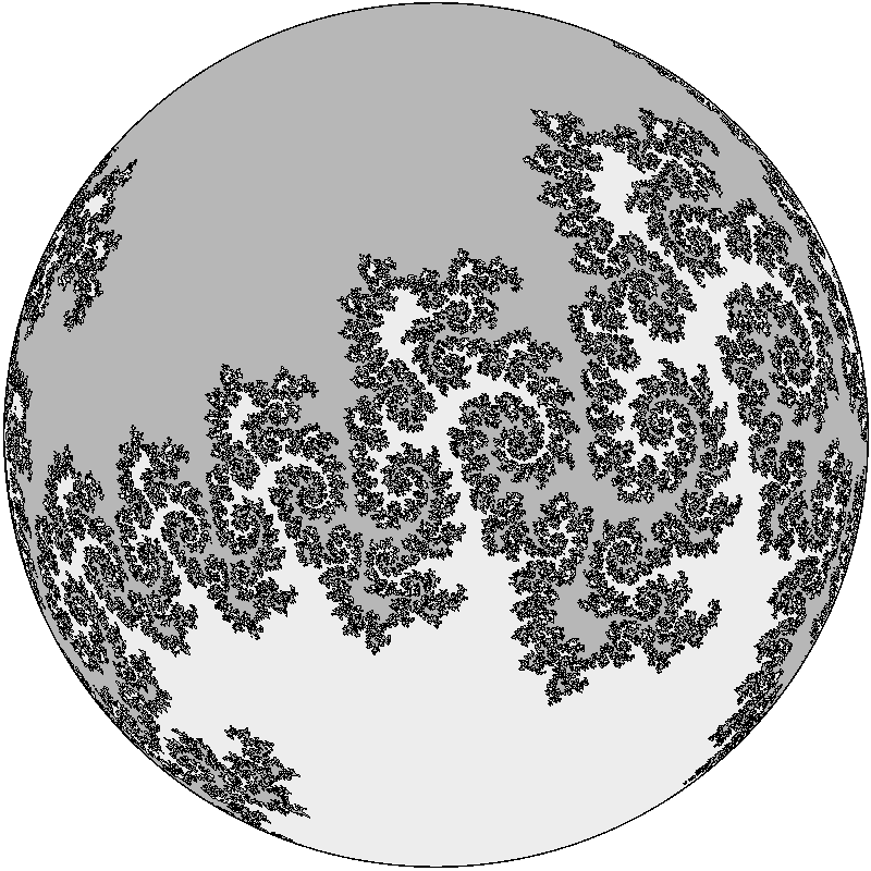
Figure 6. Julia set for a point in the $(5/11)$-fjord. This is a Jordan curve, separating the basins of zero and infinity. The left side illustrates the Riemann sphere version, and the right side shows the view in the $z$-plane, with the unit circle drawn in.

2. Fatou Components and Hyperbolic Components

We first prove the following preliminary result.

Theorem 2.1.

Let $U$ be a Fatou component for some map $f=f_{q}$ belonging to our family $(\ref{e0})$. If some forward image $f^{\circ k}(U)$ is a Herman ring, then $U$ is an annulus; but in all other cases $U$ is simply-connected. In particular, the Julia set ${\mathscr{J}}(f)$ is connected if and only if there is no Herman ring.

Proof.

First consider the special case where $U$ is a periodic Fatou component.

Case 1. A rotation domain.

If there are no critical points in this cycle of Fatou components, then $U$ must be either a Herman ring (necessarily an annulus), or a Siegel disk (necessarily simply connected). In either case there is nothing to prove. Thus we are reduced to the attracting and parabolic cases.

Case 2. An attracting domain of period $m\geq 2$.

Then $U$ contains an attracting periodic point $z_{0}$ of period $m$. Let ${\mathscr{O}}$ be the orbit of $z_{0}$, and let $U_{0}$ be a small disk about $z_{0}$ which is chosen so that $f^{\circ m}(U_{0})\subset U_{0}$, and so that the boundary $\partial U_{0}$ does not contain any postcritical point. For each $j\geq 0$, let $U_{j}$ be the connected component of $f^{-j}(U_{0})$ which contains a point of ${\mathscr{O}}$, thus $f(U_{j})=U_{j-1}$. Assuming inductively that $U_{j}$ is simply connected, we will prove that $U_{j+1}$ is also simply connected. If $U_{j+1}$ contains no critical point, then it is an unbranched covering of $U_{j}$, and hence maps diffeomorphically onto $U_{j}$. If there is only one critical point, mapping to the critical value $v\in U_{j}$, then $U_{j+1}{\smallsetminus}f^{-1}(v)$ is an unbranched covering space of $U_{j}{\smallsetminus}\{v\}$, and hence is a punctured disk. It follows again that $U_{j+1}$ is simply connected. We must show that there cannot be two critical points in $U_{j+1}$. Certainly it cannot contain either of the two fixed critical points, since the period is two or more. If it contained both free critical points, then it would intersect its antipodal image, and hence be self-antipodal. Similarly its image under $f_{q}$ would be self-antipodal. Since two connected self-antipodal sets must intersect each other, it would again follow that the period must be one, contradicting the hypothesis.

Thus it follows inductively that each $U_{j}$ is simply connected. Since the entire Fatou component $U$ is the nested union of the $U_{jm}$, it is also simply connected.∎

Case 3. A parabolic domain of period $m$.

Note first that we must have $m\geq 2$. In fact it follows from the holomorphic fixed point formula that every non-linear rational map must have either a repelling fixed point (and hence an antipodal pair of repelling points in our case) or a fixed point of multiplier $+1$. But the latter case cannot occur in our family since the two free critical points are antipodal and can never come together.

The argument is now almost the same as in the attracting case, except that in place of a small disk centered at the parabolic point, we take a small attracting petal which intersects all orbits in its Fatou component.

Remark 2.2.

In Cases 2 and 3, we will see in Theorem 6.7 that the boundary $\partial U$ is always a Jordan curve.

Case 4. An attracting domain of period one: the basin of zero or infinity.

As noted in Case 3, the two free fixed points are necessarily repelling, so the only attracting fixed points are zero and infinity.

Let us concentrate on the basin of zero. Construct the sets $U_{j}$ as in Case 2. If there are no other critical points in this immediate basin, then it follows inductively that the $U_{j}$ are all simply connected. If there is another critical point $c$ in the immediate basin, then there will be a smallest $j$ such that $U_{j+1}$ contains $c$. Consider the Riemann-Hurwitz formula

$$\chi(U_{j+1})=d\cdot\chi(U_{j})-n,$$

where $\chi(U_{j})=1$, $d$ is the degree of the map $U_{j+1}\to U_{j}$, and $n=2$ is the number of critical points in $U_{j+1}$. If $d=3$, then $U_{j+1}$ is simply connected, and again it follows inductively that the $U_{j}$ are all simply connected. However, if $d=2$ so that $U_{j+1}$ is an annulus, then we would have a more complicated situation, as illustrated in Figure 7. The two disjoint closed annuli $\overline{U}_{j+1}$ and ${\mathpzc A}(\overline{U}_{j+1})$ would separate the Riemann sphere it into two simply connected regions plus one annulus. One of these simply connected regions $E$ would have to share a boundary with $U_{j+1}$, and the antipodal region ${\mathpzc A}(E)$ would share a boundary with ${\mathpzc A}(U_{j+1})$. The remaining annulus $A$ would then share a boundary with both $U_{j+1}$ and ${\mathpzc A}(U_{j+1})$, and hence would be self-antipodal. We must prove that this case cannot occur.

Figure 7. Three concentric annuli. $($See Case $4$.$)$ The innermost annulus $U_{j+1}$, with emphasized boundary, contains the disk $U_{j}$, while the outermost annulus ${\mathpzc A}(U_{j+1})$ contains ${\mathpzc A}(U_{j})$. The annulus $A$ lies between these two. Finally, the innermost region $E$ and the outermost region ${\mathpzc A}(E)$ are topological disks.

Each of the two boundary curves of $U_{j+1}$ (emphasized in Figure 7) must map homeomorphically onto $\partial U_{j}$. Thus one of the two boundary curves of $A$ maps homeomorphically onto $\partial U_{j}$, and the other must map homeomorphically onto ${\mathpzc A}(\partial U_{j})$. Note that there are no critical points in $A$. The only possibility is that $A$ maps homeomorphically onto the larger annulus $A^{\prime}={\widehat{\mathbb{C}}}{\smallsetminus}\big{(}\overline{U}_{j}\cup{\mathpzc A}(\overline{U}_{j})\big{)}$. This behavior is perfectly possible for a branched covering, but is impossible for a holomorphic map, since the modulus of $A^{\prime}$ must be strictly larger than the modulus of $A$. This contradiction completes the proof that each periodic Fatou component is either simply connected, or a Herman ring.

The Preperiodic Case.

For any non-periodic Fatou component $U$, we know by Sullivan’s nonwandering theorem that some forward image $f^{\circ k}(U)$ is periodic. Assuming inductively that $f(U)$ is an annulus or is simply connected, we must prove the same for $U$. If $f(U)$ is simply connected, then it is easy to check that there can be at most one critical point in $U$, hence as before it follows that $U$ is simply connected. In the annulus case, the two free critical points necessarily belong to the Julia set, and hence cannot be in $U$. Therefore $U$ is a finite unbranched covering space of $f(U)$, and hence is also an annulus. This completes the proof of Theorem 2.1. ∎

The corresponding result in the parameter plane is even sharper.

Lemma 2.3.

Every hyperbolic component, either in the $q$-plane or in the $q^{2}$-plane, is simply connected, with a unique critically finite point $($called its center$)$.

Proof.

This is a direct application of results from [M5]. Theorem 9.3 of that paper states that every hyperbolic component in the moduli space for rational maps of degree $d$ with marked fixed points is a topological cell with a unique critically finite “center” point. We can also apply this result to the sub moduli space consisting of maps with one or more marked critical fixed points (Remark 9.10 of the same paper). The corresponding result for real forms of complex maps is also true. (See [M5, Theorem 7.13 and Remark 9.6].)

These results apply in our case, since we are working with a real form of the moduli space of cubic rational maps with two marked critical fixed points. The two remaining fixed points are then automatically marked: one in the upper half-plane and one in the lower half-plane. (Compare the discussion below.) ∎

Figure 8.

We will need a more precise description of the four (not necessarily distinct) critical points of $f_{q}$. The critical fixed points zero and infinity are always present, and there are also two mutually antipodal free critical points. For $q\neq 0$ we will denote the two free critical points by

$${{\bf c}_{0}}(q)=\left(\frac{a-3+\sqrt{P(a)}}{4a}\right)q\;,\quad{\rm and}\quad{{\bf c}_{\infty}}(q)=\left(\frac{a-3-\sqrt{P(a)}}{4a}\right)q\;,$$ (2)

where $a=|q^{2}|>0$ and $P(a)=9+10a+a^{2}>9$. Thus ${{\bf c}_{0}}={{\bf c}_{0}}(q)$ is a positive multiple of $q$, and ${{\bf c}_{\infty}}={{\bf c}_{\infty}}(q)$ is a negative multiple of $q$. A straightforward computation shows that $\big{(}a-3+\sqrt{P(a)}\big{)}<4a$, so ${{\bf c}_{0}}(q)$ is between $0$ and $q$. As $q$ tends to zero, ${{\bf c}_{0}}(q)$ tends to zero, and ${{\bf c}_{\infty}}(q)$ tends to infinity. For $q\neq 0$, it follows easily that the three finite critical points, as well as the zero $q\in f_{q}^{-1}(0)$ and the pole ${\mathpzc A}(q)$, all lie on a straight line, with ${{\bf c}_{0}}(q)$ between zero and $q$ and with ${\mathpzc A}(q)$ between ${{\bf c}_{\infty}}(q)$ and zero, as shown in Figure 8.

Setting $q=x+iy$, a similar computation shows that the two free fixed points are given by

$${\boldsymbol{\xi}}_{\pm}(q)=i\Big{(}y\pm\sqrt{y^{2}+1}\Big{)}\qquad{\rm where}\qquad y=\mathop{\mathrm{Im}}(q).$$ (3)

Thus ${\boldsymbol{\xi}}_{+}(q)$ always lies on the positive imaginary axis, while its antipode ${\boldsymbol{\xi}}_{-}(q)$ lies on the negative imaginary axis. As noted in the proof of Theorem 2.1, both of these free fixed points must be strictly repelling. One of the two is always on the boundary of the basin of zero, and the other is always on the boundary of the basin of infinity. More precisely, if $y>0$ then ${\boldsymbol{\xi}}_{+}(q)$ lies on the boundary of the basin of infinity and ${\boldsymbol{\xi}}_{-}(q)$ lies on the boundary of the basin of zero; while if $y<0$ then the opposite is true. (Of course if $q^{2}\in{{\pazocal H}_{0}}$, then both free fixed points lie on the common self-antipodal boundary. In particular, this happens when $y=0$.)

Figure 9. Crown at the head of the lower $(1/2)$-tongue in the $q$-plane, showing the angles of several parameter rays.

Figure 10. Detail to the upper right of Figure 10 centered at $q=.1476-1.927~{}{\rm i}$, showing a small Mandelbrot set. (Compare Figure 11.) An internal ray of angle $4/7$ (drawn in by hand) lands at the root point of this Mandelbrot set. Here ${\widetilde{\pazocal H}_{0}}$ is the white region to the right— The other white or grey regions are capture components.

Figure 11. Julia set for the center of the small Mandelbrot set of Figure10, with some internal and external angles labeled. (Compare Remark 7.4.) The unit circle has been drawn to fix the scale.

We can now give a preliminary description of the possible hyperbolic components.

Lemma 2.4.

Every hyperbolic component in the $q^{2}$-plane belongs to one of the following four types:

$\bullet$ The central hyperbolic component ${{\pazocal H}_{0}}$ (the white region in Figure 5). This is the unique component for which the Julia set is a Jordan curve, which necessarily separates the basins of zero and infinity. In this case, the critical point ${{\bf c}_{0}}(q)$ necessarily lies in the basin of zero, and ${{\bf c}_{\infty}}(q)$ lies in the basin of infinity. Compare Figures 6, 15 (left), and 17. The corresponding white region in the $q$-plane (Figure 1) is a branched 2-fold covering space, which will be denoted by ${\widetilde{\pazocal H}_{0}}$.

$\bullet$ Mandelbrot Type. Here there are two mutually antipodal attracting orbits of period two or more, with one free critical point in the immediate basin of each one. For an example in the parameter plane, see Figure 10 and for the corresponding Julia set see Figure 11.)

$\bullet$ Tricorn Type. Here there is one self antipodal attracting orbit, necessarily of even period. The most conspicuous examples are the tongues which stretch out to infinity. (These will be studied in [BBM2].) There are also small bounded tricorns. (See Figures 13 and 13.)

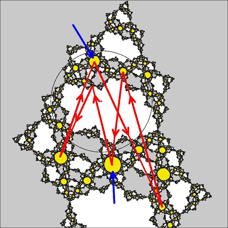
Figure 12. Magnified picture of a tiny speck in the upper right of Figure10, showing a period six tricorn centered at $q\approx 0.394-2.24i$. The white and grey regions are capture components. (For a corresponding Julia set, see Figure 13.)

Figure 13. Julia set corresponding to the small tricorn of Figure 13.

$\bullet$ Capture Type. Here the free critical points are not in the immediate basin of zero or infinity, but some forward image of each free critical point belongs in one basin or the other. (These regions are either dark grey or white in Figures 1, 5, 5, 10, 10, 13, according as the orbit of ${{\bf c}_{0}}(q)$ converges to $\infty$ or $0$.)

Proof of Lemma 2.4.

This is mostly a straightforward exercise—Since there are only two free critical points, whose orbits are necessarily antipodal to each other, there are not many possibilities. As noted in the proof of Theorem 2.1, the two fixed points in ${\mathbb{C}}{\smallsetminus}\{0\}$ must be strictly repelling. However, the uniqueness of ${{\pazocal H}_{0}}$ requires some proof. In particular, since ${{\bf c}_{0}}(q)$ can be arbitrarily large, one might guess that there could be another hyperbolic component for which ${{\bf c}_{0}}(q)$ lies in the immediate basin of infinity. We must show that this is impossible.

According to Lemma 2.3, for the center of such a hyperbolic component, the point ${{\bf c}_{0}}(q)$ would have to be precisely equal to infinity. But as ${{\bf c}_{0}}(q)$ approaches infinity, according to Equation (2) the parameter $q$ must also tend to infinity. Since$f(q)=0$ and $f(\infty)=\infty$, there cannot be any such well behaved limit.

Examples illustrating all four cases, are easily provided. (Compare the figures cited above.) ∎

3. The Central Hyperbolic Component ${{\pazocal H}_{0}}$.

As noted in Lemma 2.4, the central hyperbolic component in the $q^{2}$-plane consists of all $q^{2}$ such that the Julia set of $f_{q}$ is a Jordan curve. The critical point ${{\bf c}_{0}}(q)$ necessarily lies in the basin of zero, and ${{\bf c}_{\infty}}(q)$ in the basin of infinity.

Lemma 3.1.

The open set ${{\pazocal H}_{0}}$ in the $q^{2}$-plane is canonically diffeomorphic to the open unit disk ${\mathbb{D}}$ by the map

$${\mathfrak{b}}:{{\pazocal H}_{0}}\stackrel{{\scriptstyle\cong}}{{\longrightarrow}}{\mathbb{D}}$$

which satisfies ${\mathfrak{b}}(0)=0$ and carries each $\,q^{2}\neq 0\,$ to the Böttcher coordinate ${\mathfrak{b}}_{q}\big{(}{{\bf c}_{0}}(q)\big{)}$ of the marked critical point.

Remark 3.2.

It follows that there is a canonical way of putting a conformal structure on the open set ${{\pazocal H}_{0}}$. However, this conformal structure becomes very wild near the boundary $\partial{{\pazocal H}_{0}}$. It should be emphasized that the entire $q^{2}$-plane does not have any natural conformal structure. (The complex numbers $q$ and $q^{2}$ are not holomorphic parameters, since the value $f_{q}(z)$ does not depend holomorphically on $q$.)

Proof of Lemma 3.1.

The proof will depend on results from [M5]. (See in particular Theorem 9.3 and Remark 9.10 in that paper.) In order to apply these results, we must work with polynomials or rational maps with marked fixed points.

First consider cubic polynomials of the form

$$p_{a}(z)=z^{3}+az^{2}$$

with critical fixed points at zero and infinity. Let ${\widetilde{\pazocal H}_{0}^{\rm poly}}$ be the principal hyperbolic component consisting of values of $a$ such that both critical points of $p_{a}$ lie in the immediate basin of zero. This set is simply-connected and contains no parabolic points, hence each of the two free fixed points can be defined as a holomorphic function ${\gamma}_{\pm}(a)$ for $a$ in ${\widetilde{\pazocal H}_{0}^{\rm poly}}$, with ${\gamma}_{\pm}(0)=\pm 1$. The precise formula is

$${\gamma}_{\pm}(a)=\frac{-a\pm\sqrt{a^{2}+4}}{2}.$$

Similarly, let ${\widetilde{\pazocal H}_{0}^{\rm rat}}$ denote the principal hyperbolic component in the space of cubic rational maps of the form

$$f_{b,c}(z)=z^{2}\frac{z+b}{cz+1}$$

with critical fixed points at zero and infinity. This is again simply-connected. Therefore the two free fixed points can be expressed as holomorphic functions ${\xi}_{\pm}(b,c)$ with ${\xi}_{\pm}(0,0)=\pm 1$.

The basic result in [M5] implies that ${\widetilde{\pazocal H}_{0}^{\rm rat}}$ is naturally biholomomorphic to the Cartesian product ${\widetilde{\pazocal H}_{0}^{\rm poly}}\!\times{\widetilde{\pazocal H}_{0}^{\rm poly}}$, where a given pair $(p_{a_{1}},p_{a_{2}})\in{\widetilde{\pazocal H}_{0}^{\rm poly}}\!\times{\widetilde{\pazocal H}_{0}^{\rm poly}}$ corresponds to the map $f_{b,c}\in{\widetilde{\pazocal H}_{0}^{\rm rat}}$ if and only if:

(1) the map $f_{b,c}$ restricted to its basin of zero is holomorphically conjugate to the map $p_{a_{1}}$ restricted to its basin of zero, with the boundary fixed point ${\xi}_{+}(b,c)$ corresponding to ${\gamma}_{+}(a_{1})$; and

(2) $f_{b,c}$ restricted to its basin of infinity is holomorphically conjugate to $p_{a_{2}}$ restricted to its basin of zero, with the boundary fixed point ${\xi}_{+}(b,c)$ corresponding to ${\gamma}_{+}(a_{2})$.

Now let ${{\pazocal H}_{0}^{\rm poly}}$ be the moduli space obtained from ${\widetilde{\pazocal H}_{0}^{\rm poly}}$ by identifying each $p_{a}$ with $p_{-a}$. According to [M4, Lemma 3.6], the correspondence which maps $p_{a}$ to the Böttcher coordinate of its free critical point gives rise to a conformal isomorphism between ${{\pazocal H}_{0}^{\rm poly}}$ and the open unit disk.

Note that our space ${\widetilde{\pazocal H}_{0}}$ is embedded real analytically as the subspace of ${\widetilde{\pazocal H}_{0}^{\rm rat}}$ consisting of maps $f_{q}$ which commute with the antipodal map. Since $f_{q}$ restricted to the basin of infinity is anti-conformally conjugate to $f_{q}$ restricted to the basin of zero, it follows easily that each $f_{q}\in{\widetilde{\pazocal H}_{0}}\subset{\widetilde{\pazocal H}_{0}^{\rm rat}}$ must correspond to a pair of the form $(p_{a},p_{\pm\bar{a}})\in{\widetilde{\pazocal H}_{0}^{\rm poly}}\times{\widetilde{\pazocal H}_{0}^{\rm poly}}$, for some choice of sign. In fact the correct sign is $(p_{a},p_{-\bar{a}})$. (The other choice of sign $(p_{a},p_{\bar{a}})$ would yield maps invariant under an antiholomorphic involution with an entire circle of fixed points, conjugate to the involution $z\leftrightarrow\overline{z}$.)

It follows that the composition of the real analytic embedding

$${\widetilde{\pazocal H}_{0}}\hookrightarrow{\widetilde{\pazocal H}_{0}^{\rm rat}}\cong{\widetilde{\pazocal H}_{0}^{\rm poly}}\times{\widetilde{\pazocal H}_{0}^{\rm poly}}$$

with the holomorphic projection to the first factor ${\widetilde{\pazocal H}_{0}^{\rm poly}}$ is a real analytic diffeomorphism ${\widetilde{\pazocal H}_{0}}\stackrel{{\scriptstyle\cong}}{{\longrightarrow}}{\widetilde{\pazocal H}_{0}^{\rm poly}}$ (but is not a conformal isomorphism). The corresponding assertion for ${{\pazocal H}_{0}}\stackrel{{\scriptstyle\cong}}{{\longrightarrow}}{{\pazocal H}_{0}^{\rm poly}}\cong{\mathbb{D}}$ follows easily. This completes the proof of Lemma 3.1. ∎

Remark 3.3.

(Compare [M6], [ShTL] and [MP].) Let $f$ and $g$ be (not necessarily distinct) monic cubic polynomials. Each one has a unique continuous extension to the circled plane, such that each point on the circle at infinity is mapped to itself by the angle tripling map ${\boldsymbol{\infty}}_{\bf t}\mapsto{\boldsymbol{\infty}}_{3t}$. Let $\raisebox{-1.49994pt}{\includegraphics[width=9.39545pt]{cc-crop.pdf}}_{f}\uplus\raisebox{-1.49994pt}{\includegraphics[width=9.39545pt]{cc-crop.pdf}}_{g}$ be the topological sphere obtained from the disjoint union $\raisebox{-1.49994pt}{\includegraphics[width=9.39545pt]{cc-crop.pdf}}_{f}\sqcup\raisebox{-1.49994pt}{\includegraphics[width=9.39545pt]{cc-crop.pdf}}_{g}$ of two copies of the circled plane by gluing the two boundary circles together, identifying each point ${\boldsymbol{\infty}}_{\bf t}\in\partial\raisebox{-1.49994pt}{\includegraphics[width=9.39545pt]{cc-crop.pdf}}_{f}$ with the point ${\boldsymbol{\infty}}_{-{\bf t}}\in\partial\raisebox{-1.49994pt}{\includegraphics[width=9.39545pt]{cc-crop.pdf}}_{g}$. Then the extension of $f$ to $\raisebox{-1.49994pt}{\includegraphics[width=9.39545pt]{cc-crop.pdf}}_{f}$ and the extension of $g$ to $\raisebox{-1.49994pt}{\includegraphics[width=9.39545pt]{cc-crop.pdf}}_{g}$ agree on the common boundary, yielding a continuous map $f\uplus g$ from the sphere $\raisebox{-1.49994pt}{\includegraphics[width=9.39545pt]{cc-crop.pdf}}_{f}\uplus\raisebox{-1.49994pt}{\includegraphics[width=9.39545pt]{cc-crop.pdf}}_{g}$ to itself.

Now assume that the Julia sets of $f$ and $g$ are locally connected. Let$K(f)\perp\!\!\perp K(g)$ be the quotient space obtained from the disjoint union $K(F)\sqcup K(g)$ by identifying the landing point of the $t$-ray on the Julia set $\partial K(f)$ with the landing point of the $-t$-ray on $\partial K(g)$ for each $t$. Equivalently, $K(F)\perp\!\!\perp K(g)$ can be described as the quotient space of the sphere $\raisebox{-1.49994pt}{\includegraphics[width=9.39545pt]{cc-crop.pdf}}_{f}\uplus\raisebox{-1.49994pt}{\includegraphics[width=9.39545pt]{cc-crop.pdf}}_{g}$ in which the closure of every dynamic ray in $\raisebox{-1.49994pt}{\includegraphics[width=9.39545pt]{cc-crop.pdf}}_{f}{\smallsetminus}K(f)$ or in $\raisebox{-1.49994pt}{\includegraphics[width=9.39545pt]{cc-crop.pdf}}_{g}{\smallsetminus}K(g)$ is collapsed to a point.

In many cases (but not always), this quotient space is a topological 2-sphere. In these cases, the topological mating $f\perp\!\!\perp g$ is defined to be the induced continuous map from this quotient 2-sphere to itself. Furthermore in many cases (but not always) the quotient sphere has a unique conformal structure satisfying the following three conditions:

(1) The map $f\perp\!\!\perp g$ is holomorphic (and hence rational) with respect to this structure.

(2) This structure is compatible with the given conformal structures on the interiors of $K(f)$ and $K(g)$ whenever these interiors are non-empty.

(3) The natural map from $\raisebox{-1.49994pt}{\includegraphics[width=9.39545pt]{cc-crop.pdf}}_{f}\uplus\raisebox{-1.49994pt}{\includegraphics[width=9.39545pt]{cc-crop.pdf}}_{g}$ to $K(f)\perp\!\!\perp K(g)$ has degree one.

When these conditions are satisfied, the resulting rational map is described as the conformal mating of $f$ and $g$.

In order to study matings which commute with the antipodal map of the Riemann sphere, the first step is define an appropriate antipodal map ${\mathscr{A}}$ from the intermediate sphere $\raisebox{-1.49994pt}{\includegraphics[width=9.39545pt]{cc-crop.pdf}}_{f}\uplus\raisebox{-1.49994pt}{\includegraphics[width=9.39545pt]{cc-crop.pdf}}_{g}$ to itself. In fact, writing the two maps as $z\mapsto f(z)$ and $w\mapsto g(w)$, define the involution ${\mathscr{A}}:\raisebox{-1.49994pt}{\includegraphics[width=9.39545pt]{cc-crop.pdf}}_{f}\longleftrightarrow\raisebox{-1.49994pt}{\includegraphics[width=9.39545pt]{cc-crop.pdf}}_{g}$ by

$${\mathscr{A}}:z\longleftrightarrow w=-\overline{z}.$$

Evidently ${\mathscr{A}}$ is well defined and antiholomorphic, with no fixed points outside of the common circle at infinity. On the circle at infinity, it sends $z={\boldsymbol{\infty}}_{\bf t}$ to $w=-{\boldsymbol{\infty}}_{-{\bf t}}$. Since each $z={\boldsymbol{\infty}}_{\bf t}$ is identified with $w={\boldsymbol{\infty}}_{-{\bf t}}$, this corresponds to a 180^∘ rotation of the circle, with no fixed points.

Now suppose that the intermediate map $f\uplus g$ from $\raisebox{-1.49994pt}{\includegraphics[width=9.39545pt]{cc-crop.pdf}}_{f}\uplus\raisebox{-1.49994pt}{\includegraphics[width=9.39545pt]{cc-crop.pdf}}_{g}$ to itself commutes with ${\mathscr{A}}$,

$${\mathscr{A}}\circ(f\uplus g)=(f\uplus g)\circ{\mathscr{A}}.$$

It is easy to check that this is equivalent to the requirement that

$$g(-\overline{z})=-\overline{f(z)},$$

or that $g(z)=-\overline{f(-\overline{z})}.$ In the special case $f(z)=z^{3}+az^{2}$, it corresponds to the condition that

$$g(z)=z^{3}-\overline{a}z^{2}.$$

Next suppose that the topological mating $f\perp\!\!\perp g$ exists. Then it is not hard to see that ${\mathscr{A}}$ gives rise to a corresponding map ${\mathscr{A}}^{\prime}$ of topological degree $-1$ from the sphere $K(f)\uplus K(g)$ to itself. If ${\mathscr{A}}^{\prime}$ had a fixed point $\bf x$, then there would exist a finite chain $C$ of dynamic rays in $\raisebox{-1.49994pt}{\includegraphics[width=9.39545pt]{cc-crop.pdf}}_{f}\uplus\raisebox{-1.49994pt}{\includegraphics[width=9.39545pt]{cc-crop.pdf}}_{g}$ leading from a representative point for $\bf x$ to its antipode. This is impossible, since it would imply that the union $C\cup{\mathscr{A}}(C)$ is a closed loop separating the sphere $\raisebox{-1.49994pt}{\includegraphics[width=9.39545pt]{cc-crop.pdf}}_{f}\uplus\raisebox{-1.49994pt}{\includegraphics[width=9.39545pt]{cc-crop.pdf}}_{g}$, which would imply that the quotient $K(f)\uplus K(g)$ is not a topological sphere, contrary to hypothesis.

Finally, if the conformal mating exists, we will show that the fixed point free involution ${\mathscr{A}}^{\prime}$ is anti-holomorphic. To see this, note that the invariant conformal structure $\Sigma$ can be transported by ${\mathscr{A}}^{\prime}$ to yield a new complex structure ${\mathscr{A}}^{\prime}_{*}(\Sigma)$ which is still invariant, but has the opposite orientation. Since we have assumed that $\Sigma$ is the only conformal structure satisfying the conditions (1), (2), (3), it follows that ${\mathscr{A}}^{\prime}_{*}(\Sigma)$ must coincide with the complex conjugate conformal structure $\overline{\Sigma}$. This is just another way of saying that ${\mathscr{A}}^{\prime}$ is antiholomorphic.

In fact, all maps $f_{q}$ in ${\widetilde{\pazocal H}_{0}}$ can be obtained as matings. Furthermore, Sharland [S] has shown that many maps outside of ${\widetilde{\pazocal H}_{0}}$ can also be described as matings.

Definition 3.4.

Using this canonical dynamically defined diffeomorphism ${\mathfrak{b}}$, each internal angle ${\boldsymbol{\vartheta}}\in{{\mathbb{R}}/{\mathbb{Z}}}$ determines a parameter ray

$${\pazocal R}_{\boldsymbol{\vartheta}}={\mathfrak{b}}^{-1}\bigl{(}\{re^{2\pi i{\boldsymbol{\vartheta}}};0<r<1\}\bigr{)}\subset{{\pazocal H}_{0}}{\smallsetminus}\{0\}.$$

(These are stretching rays in the sense of Branner-Hubbard, see [B], [BH] and [T]. In particular, any two maps along a common ray are quasiconformally conjugate to each other.)

Theorem 3.5.

If the angle ${\boldsymbol{\vartheta}}\in{\mathbb{Q}}/{\mathbb{Z}}$ is periodic under doubling, then the parameter ray ${\pazocal R}_{\boldsymbol{\vartheta}}$ either:

• lands at a parabolic point on the boundary $\partial{{\pazocal H}_{0}}$,

• accumulates on a curve of parabolic boundary points, or

• lands at a point ${\boldsymbol{\infty}}_{\bf t}$ on the circle at infinity, where ${\bf t}$ can be described as the rotation number of ${\boldsymbol{\vartheta}}$ under angle doubling.

Here Cases (a) and (c) can certainly occur. (See Figures 10 and 25.) For Case (b), numerical computations by Hiroyuki Inou suggest strongly that rays can accumulate on a curve of parabolic points without actually landing (indicated schematically in Figure 10). This will be studied further in [BBM2]. For the analogous case of multicorns see [IM].

Remark 3.6.

In case (b), we will show in [BBM2] that the orbit is bounded away from the circle at infinity. If the angle ${\boldsymbol{\vartheta}}$ is rational but not periodic, then we will show that ${\pazocal R}_{\boldsymbol{\vartheta}}$ lands on a critically finite parameter value.

The proof of Theorem 3.5 will make use of the following definitions.

Let ${\mathscr{B}}_{q}$ be the immediate basin of zero for the map $f_{q}$. In the case $q^{2}\not\in{{\pazocal H}_{0}}$, note that the Böttcher coordinate is well defined as a conformal isomorphism ${\mathfrak{b}}_{q}:{\mathscr{B}}_{q}\stackrel{{\scriptstyle\cong}}{{\longrightarrow}}{\mathbb{D}}$ satisfying

$${\mathfrak{b}}_{q}\big{(}f_{q}(z)\big{)}=\bigl{(}{\mathfrak{b}}_{q}(z)\bigr{)}^{2}.$$

Radial lines in the open unit disk ${\mathbb{D}}$ then correspond to dynamic internal rays ${\mathscr{R}}_{q,\theta}:[0,1)\to{\mathscr{B}}_{q}$, where $\theta$ is the internal angle in ${\mathbb{D}}$. As in the polynomial case every periodic ray lands on a periodic point.

However, for the moment we are rather concerned with the case $q^{2}\in{{\pazocal H}_{0}}{\smallsetminus}\{0\}$. In this case, ${\mathfrak{b}}_{q}$ is defined only on a open subset of ${\mathscr{B}}_{q}$. More precisely, ${\mathfrak{b}}_{q}$ is certainly well defined as a conformal isomorphism from a neighborhood of zero in ${\mathscr{B}}_{q}$ to a neighborhood of zero in ${\mathbb{D}}$. Furthermore the correspondence $z\mapsto|{\mathfrak{b}}_{q}(z)|^{2}$ extends to a well defined smooth map from ${\mathscr{B}}_{q}$ onto $[0,1)$. The dynamic internal rays can then be defined as the orthogonal trajectories of the equipotential curves $|{\mathfrak{b}}_{q}(z)|^{2}={\rm constant}$. The difficulty is that this map $z\mapsto|{\mathfrak{b}}_{q}(z)|^{2}$ has critical points at every critical or precritical point of $f_{q}$; and that countably many of the internal rays will bifurcate off these critical or precritical points. However, every internal ray outside of this countable set is well defined as an injective map ${\mathscr{R}}_{q,\theta}:[0,1)\to{\mathscr{B}}_{q}$, and has a well defined landing point in $\partial{\mathscr{B}}_{q}={\mathscr{J}}(f_{q})$.

The notation ${{\mathscr{B}}_{q}^{\rm vis}}$ will be used for the open subset of ${\mathscr{B}}_{q}$ consisting of all points which are directly visible from the origin in the sense that there is a smooth internal ray segment from the origin which passes through the point. The topological closure $\overline{{\mathscr{B}}_{q}^{\rm vis}}$ will be called the set of visible points.

For $q^{2}\in{{\pazocal H}_{0}}{\smallsetminus}\{0\}$, the map ${\mathfrak{b}}_{q}$ sends the set of directly visible points ${{\mathscr{B}}_{q}^{\rm vis}}$ univalently onto a proper open subset of ${\mathbb{D}}$ which is obtained from the open disk by removing countably many radial slits near the boundary. (See Figure 14.) These correspond to the countably many internal rays from the origin in ${\mathscr{B}}_{q}$ which bifurcate off critical or precritical points.

Figure 14. On the left: the basin ${\mathscr{B}}_{q}$. In this example, $q>0$ so that the critical point ${{\bf c}_{0}}(q)$ is on the positive real axis. Points which are visible from the origin are shown in dark gray, and the two critical points in ${\mathscr{B}}_{q}$ are shown as black dots. On the right: a corresponding picture in the disk of Böttcher coordinates. Note that the light grey regions on the left correspond only to slits on the right.

Proof of Theorem 3.5.

Suppose that ${\boldsymbol{\vartheta}}$ has period $n\geq 1$ under doubling. Let $\{q^{2}_{k}\}$ be a sequence of points on the parameter ray ${\pazocal R}_{\boldsymbol{\vartheta}}\subset{{\pazocal H}_{0}}$, converging to a limit $q^{2}\in\partial{{\pazocal H}_{0}}$ in the finite $q^{2}$-plane. Choose representatives $q_{k}=\pm\sqrt{q^{2}_{k}}$, converging to a limit $q$. Since ${\boldsymbol{\vartheta}}$ is periodic and $q^{2}\not\in{{\pazocal H}_{0}}$, the internal dynamic ray ${\mathscr{R}}_{q,{\boldsymbol{\vartheta}}}$ lands on a periodic point $z_{q}=f_{q}^{\circ n}(z_{q})$. If this landing point were repelling, then every nearby ray ${\mathscr{R}}_{q_{k},{\boldsymbol{\vartheta}}}$ would have to land on a nearby repelling point of $f_{q_{k}}$. But this is impossible, since each ${\mathscr{R}}_{q_{k},{\boldsymbol{\vartheta}}}$ must bifurcate. Thus $z_{q}$ must be a parabolic point.

Since the ray ${\mathscr{R}}_{q,{\boldsymbol{\vartheta}}}$ landing on $z_{q}$ has period $n$, we say that this point $z_{q}$ has ray period $n$. Equivalently, each connected component of the immediate parabolic basin of $z_{q}$ has exact period $n$. If the period of $z_{q}$ under $f_{q}$ is $p$, note that the multiplier of $f_{q}^{\circ p}$ at $z_{q}$ must be a primitive $(n/p)$-th root of unity. (Compare [GM, Lemma 2.4].) The set of all parabolic points of ray period $n$ forms a real algebraic subset of the $s$-plane. Hence each connected component is either a one-dimensional real algebraic curve or an isolated point. Since the set of all accumulation points of the parameter ray ${\pazocal R}_{\boldsymbol{\vartheta}}$ is necessarily connected, the only possibilities are that it lands at a parabolic point or accumulates on a possibly unbounded connected subset of a curve of parabolic points. (In fact, we will show in [BBM2] that this accumulation set is always bounded.)

Now suppose that the sequence $\{q^{2}_{k}\}$ converges to a point on the circle at infinity. It will be convenient to introduce a new coordinate $u=z/q$ in place of $z$ for the dynamic plane. The map $f_{q}$ will then be replaced by the map

$$u\mapsto\frac{f_{q}(uq)}{q}=\frac{q^{2}u^{2}(1-u)}{1+|q^{2}|u}.$$

Dividing numerator and denominator by $|q^{2}|u$, and setting $\lambda=q^{2}/|q^{2}|$ and $b=1/|q^{2}|$, this takes the form

$$u\mapsto~{}g_{\lambda,b}(u)=\frac{\lambda u(1-u)}{1+b/u},$$

with $|\lambda|=1$ and $b>0$. The virtue of this new form is that the sequence of maps $g_{\lambda_{k},b_{k}}$ associated with $\{q^{2}_{k}\}$ converges to a well defined limit $P_{\lambda}(u)=\lambda u(1-u)$ as $b\to 0$, or in other words as $|q^{2}|\to\infty$. (Compare Figure 15.) Furthermore, the convergence is locally uniform for $u\in{\mathbb{C}}{\smallsetminus}\{0\}$. Note that $u=0$ is a fixed point of multiplier $\lambda$ for $P_{\lambda}$. A quadratic polynomial can have at most one non-repelling periodic orbit. (This is an easy case of the Fatou-Shishikura inequality.) Hence it follows that all other periodic orbits of $P_{\lambda}$ are strictly repelling.

 

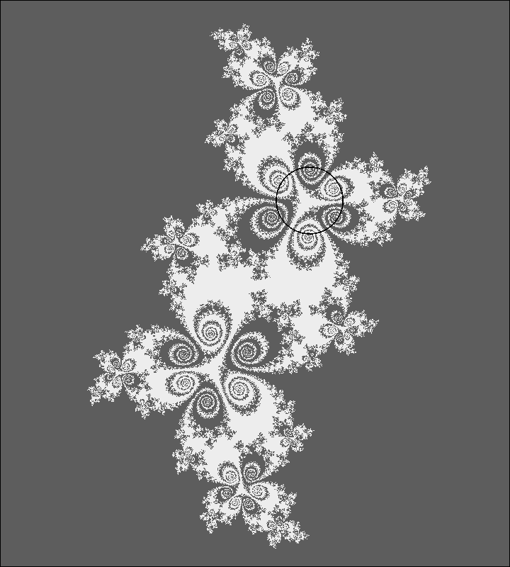
Figure 15. On the left: Julia set for a map $f_{q}$ on the $2/7$ ray. The limit of this Julia set as we tend to infinity along the $2/7$ ray, suitably rescaled and rotated, would be the Julia set for the quadratic map $w\mapsto e^{2\pi it}w(1-w)$, as shown on the right. Here $t=1/3$ is the rotation number of $2/7$ under angle doubling. In this infinite limit, the unit circle $($drawn in on the left$)$ shrinks to the parabolic fixed point.

Since ${\boldsymbol{\vartheta}}$ is a periodic angle, the external ray of angle ${\boldsymbol{\vartheta}}$ for the polynomial $P_{\lambda}$ must land at some periodic point. In fact, we claim that it must land at the origin. For otherwise it would land at a repelling point. We can then obtain a contradiction, just as in the preceding case. Since the maps $g_{\lambda_{k},b_{k}}$ converge to $P_{\lambda}$ locally uniformly on ${\widehat{\mathbb{C}}}{\smallsetminus}\{0\}$ the corresponding Böttcher coordinates in the basin of infinity also converge locally uniformly, and hence the associated external rays converge. Hence it would follow that the rays of angle ${\boldsymbol{\vartheta}}$ from infinity for the maps $g_{\lambda_{k},b_{k}}$ would also land on a repelling point for large $k$. But this is impossible since, as in the previous case, these rays must bifurcate.

This proves that the external ray of angle ${\boldsymbol{\vartheta}}$ for the quadratic map $P_{\lambda}$ lands at zero. The Snail Lemma then implies that the map $P_{\lambda}$ is parabolic, or in other words that $\lambda$ has the form $e^{2\pi i{\bf t}}$ for some rational ${\bf t}$. It follows that the angle ${\boldsymbol{\vartheta}}$ has a well defined rotation number, equal to ${\bf t}$, under angle doubling. Now recalling that $\lambda_{k}\to\lambda$ where $\lambda_{k}=s_{k}/|s_{k}|$, it follows that $s_{k}$ must converge to the point ${\boldsymbol{\infty}}_{\bf t}$ as $k\to\infty$. If the ${\boldsymbol{\vartheta}}$-ray has no accumulation points in the finite plane, then it follows that this ray actually lands at the point ${\boldsymbol{\infty}}_{\bf t}$. This completes the proof of Theorem 3.5. ∎

The following closely related lemma will be useful in §7.

Lemma 3.7.

If $q^{2}\in\partial{{\pazocal H}_{0}}$ is a finite accumulation point for the periodic parameter ray ${\pazocal R}_{\boldsymbol{\vartheta}}$ with ${\boldsymbol{\vartheta}}$ of period $n$ under doubling, then the dynamic internal ray of angle ${\boldsymbol{\vartheta}}$ in ${\mathscr{B}}_{q}$ lands at a parabolic point of ray period $n$.

Proof.

This follows from the discussion above.∎

4. Visible Points for Maps in ${{\pazocal H}_{0}}$.

If $q^{2}\in{{\pazocal H}_{0}}$, then, $f_{q}$ is in the same hyperbolic component as $f_{0}(z)=-z^{3}$. It follows that $f_{q}~{}$ on its Julia set is topologically conjugate to $f_{0}$ on its Julia set (the unit circle). As a consequence, there is a homeomorphism ${\boldsymbol{\eta}}_{q}:{{\mathbb{R}}/{\mathbb{Z}}}\to{\mathscr{J}}(f_{q})$ conjugating the tripling map ${\bf m}_{3}:x\mapsto 3x$ to $f_{q}$:

$${\boldsymbol{\eta}}_{q}\circ{\bf m}_{3}=f_{q}\circ{\boldsymbol{\eta}}_{q}\qquad\text{on}\quad{{\mathbb{R}}/{\mathbb{Z}}}.$$

This conjugacy is uniquely defined up to orientation, and up to the involution $x\leftrightarrow x+1/2$ of the circle. Note that the two fixed points $x=0$ and $x=1/2$ of the tripling map correspond to the two fixed points ${\boldsymbol{\eta}}_{q}(0)$ and ${\boldsymbol{\eta}}_{q}(1/2)$ on the Julia set. We will always choose the orientation so that ${\boldsymbol{\eta}}_{q}(x)$ travels around the Julia set in the positive direction as seen from the origin as $x$ increases from zero to one.

Assume $q^{2}\in{\pazocal R}_{\boldsymbol{\vartheta}}$ and set

$${{\Lambda}_{\boldsymbol{\vartheta}}}=\bigl{\{}\theta\in{{\mathbb{R}}/{\mathbb{Z}}}~{};~{}\forall m\geq 0,~{}2^{m}\theta\neq{\boldsymbol{\vartheta}}\bigr{\}}.$$

If $\theta\in{{\Lambda}_{\boldsymbol{\vartheta}}}$, the dynamic ray ${\mathscr{R}}_{q,\theta}$ is smooth and lands at some point ${\boldsymbol{\zeta}}_{q}(\theta)\in{\mathscr{J}}(f_{q})$. If $\theta\not\in{{\Lambda}_{\boldsymbol{\vartheta}}}$, the dynamic ray ${\mathscr{R}}_{q,\theta}$ bifurcates and we define

$${\boldsymbol{\zeta}}_{q}^{\pm}(\theta)=\lim{\boldsymbol{\zeta}}_{q}(\theta\pm\varepsilon)\quad\text{as}\quad\varepsilon\searrow 0\quad\text{with}\quad\theta\pm\varepsilon\in{{\Lambda}_{\boldsymbol{\vartheta}}}.$$

The limit exists since ${\mathscr{J}}(f_{q})$ is a Jordan curve and ${\boldsymbol{\zeta}}_{q}$ preserves the cyclic ordering.

We will choose ${\boldsymbol{\eta}}_{q}:{{\mathbb{R}}/{\mathbb{Z}}}\to{\mathscr{J}}(f_{q})$ so that

$${\boldsymbol{\eta}}_{q}(0)={\boldsymbol{\zeta}}_{q}(0)\text{ when }{\boldsymbol{\vartheta}}\neq 0\quad\text{and}\quad{\boldsymbol{\eta}}_{q}(0)={\boldsymbol{\zeta}}_{q}^{-}(0)\text{ when }{\boldsymbol{\vartheta}}=0.$$

Remark 4.1.

For each fixed $\theta\,$, as $q$ varies along some stretching ray ${\pazocal R}_{\boldsymbol{\vartheta}}$, the angle ${\boldsymbol{\eta}}_{q}^{-1}\bigl{(}{\boldsymbol{\zeta}}_{q}(\theta)\bigr{)}$ does not change (and thus, only depends on ${\boldsymbol{\vartheta}}$ and $\theta$). Indeed, ${\boldsymbol{\eta}}_{q}$ depends continuously on $q$. In addition, $\theta$ is periodic of period $p$ for the doubling map ${\bf m}_{2}:\theta\mapsto 2\theta$ if and only if ${\boldsymbol{\zeta}}_{q}(\theta)$ is periodic of period $p$ for $f_{q}$, so if and only if ${\boldsymbol{\eta}}_{q}^{-1}\bigl{(}{\boldsymbol{\zeta}}_{q}(\theta)\bigr{)}$ is periodic of period $p$ for ${\bf m}_{3}$. The result follows since the set of periodic points of ${\bf m}_{3}$ and the set of non periodic points are both totally disconnected.

Let ${\mathscr{V}}_{q}\subset{\mathscr{J}}(f_{q})$ be the closure of the set of landing points of smooth internal rays. This is also the set of visible points in ${\mathscr{J}}(f_{q})$. Our goal is to describe the set

$${V_{\boldsymbol{\vartheta}}}={\boldsymbol{\eta}}_{q}^{-1}({\mathscr{V}}_{q})\subset{{\mathbb{R}}/{\mathbb{Z}}}$$

in terms of ${\boldsymbol{\vartheta}}$ and compute, for $q^{2}\in{\pazocal R}_{\boldsymbol{\vartheta}}$,

$$\begin{cases}{\boldsymbol{{\varphi}}}_{\boldsymbol{\vartheta}}(\theta)={\boldsymbol{\eta}}_{q}^{-1}\circ{\boldsymbol{\zeta}}_{q}(\theta)&\text{if}\quad\theta\in{{\Lambda}_{\boldsymbol{\vartheta}}}\\ {\boldsymbol{{\varphi}}}_{\boldsymbol{\vartheta}}^{\pm}(\theta)={\boldsymbol{\eta}}_{q}^{-1}\circ{\boldsymbol{\zeta}}_{q}^{\pm}(\theta)&\text{if}\quad\theta\not\in{{\Lambda}_{\boldsymbol{\vartheta}}}.\end{cases}$$

We will prove the following:

Theorem 4.2.

Given ${\boldsymbol{\vartheta}}\in[0,1)$, set $\theta_{\rm min}=\min({\boldsymbol{\vartheta}},1/2)$ and $\theta_{\rm max}=\max({\boldsymbol{\vartheta}},1/2)$, so that $0\leq\theta_{\rm min}\leq\theta_{\rm max}<1$.

• If $\theta\in{{\Lambda}_{\boldsymbol{\vartheta}}}$, then

  $${\boldsymbol{{\varphi}}}_{\boldsymbol{\vartheta}}(\theta)=\frac{x_{1}}{3}+\frac{x_{2}}{9}+\frac{x_{3}}{27}+\cdots,$$

  where $x_{m}$ takes the value $0$, $1$, or $2$ according as the angle $2^{m}\theta$ belongs to the interval $[0,\theta_{\rm min})$, $[\theta_{\rm min},\theta_{\rm max})$ or $[\theta_{\rm max},1)$ modulo ${\mathbb{Z}}$.

• If $\theta\not\in{{\Lambda}_{\boldsymbol{\vartheta}}}$, the same algorithm yields ${\boldsymbol{{\varphi}}}_{\boldsymbol{\vartheta}}^{+}(\theta)$, whereas

  $${\boldsymbol{{\varphi}}}_{\boldsymbol{\vartheta}}^{-}(\theta)=\frac{x^{\prime}_{1}}{3}+\frac{x^{\prime}_{2}}{9}+\frac{x^{\prime}_{3}}{27}+\cdots,$$

  where $x^{\prime}_{m}$ takes the value $0$, $1$, or $2$ according as the angle $2^{m}\theta$ belongs to the interval $(0,\theta_{\rm min}]$, $(\theta_{\rm min},\theta_{\rm max}]$ or $(\theta_{\rm max},1]$ modulo ${\mathbb{Z}}$. In addition

  $${\boldsymbol{{\varphi}}}_{\boldsymbol{\vartheta}}^{+}(\theta)-{\boldsymbol{{\varphi}}}_{\boldsymbol{\vartheta}}^{-}(\theta)=\sum_{\{m~{};~{}2^{m}\theta={\boldsymbol{\vartheta}}\}}\frac{1}{3^{m+1}}.$$

The set ${V_{\boldsymbol{\vartheta}}}$ is the Cantor set of angles whose orbit under tripling avoids the critical gap ${{G}_{\boldsymbol{\vartheta}}}=\bigl{(}{\boldsymbol{{\varphi}}}_{\boldsymbol{\vartheta}}^{-}({\boldsymbol{\vartheta}}),{\boldsymbol{{\varphi}}}_{\boldsymbol{\vartheta}}^{+}({\boldsymbol{\vartheta}})\bigr{)}$. The critical gap ${{G}_{\boldsymbol{\vartheta}}}$ has length

$$\ell({{G}_{\boldsymbol{\vartheta}}})=\begin{cases}1/3&\text{ when }{\boldsymbol{\vartheta}}\text{ is not periodic for }{\bf m}_{2}\quad and\\ 3^{p-1}/(3^{p}-1)\in(1/3,1/2]&\text{ when }{\boldsymbol{\vartheta}}\text{ is periodic of period }p\geq 1.\end{cases}$$

Remark 4.3.

It might seem that the expression for ${\boldsymbol{{\varphi}}}_{\boldsymbol{\vartheta}}$ should have a discontinuity whenever $2^{m}\theta=1/2$, and hence $2^{n}\theta=0$ for $n>m$, but a brief computation shows that the discontinuity in $x_{m}/3^{m}$ is precisely canceled out by the discontinuity in $x_{m+1}/3^{m+1}+\cdots$.

Corollary 4.4.

The left hand endpoint $a({\boldsymbol{\vartheta}})={\boldsymbol{{\varphi}}}_{\boldsymbol{\vartheta}}^{-}({\boldsymbol{\vartheta}})$ of ${{G}_{\boldsymbol{\vartheta}}}$ is continuous from the left as a function of ${\boldsymbol{\vartheta}}$. Similarly, the right hand endpoint $b({\boldsymbol{\vartheta}})={\boldsymbol{{\varphi}}}_{\boldsymbol{\vartheta}}^{+}({\boldsymbol{\vartheta}})$ is continuous from the right. Both $a({\boldsymbol{\vartheta}})$ and $b({\boldsymbol{\vartheta}})$ are monotone as functions of ${\boldsymbol{\vartheta}}$.

Proof.

This follows easily from the formulas in Theorem 4.2. ∎

Proof of Theorem 4.2.

In the whole proof, we assume $q^{2}\in{\pazocal R}_{\boldsymbol{\vartheta}}$. If an internal ray ${\mathscr{R}}_{q,\theta}$ lands at ${\boldsymbol{\zeta}}_{q}(\theta)$, then the image ray ${\mathscr{R}}_{q,2\theta}$ lands at ${\boldsymbol{\zeta}}_{q}(2\theta)=f_{q}\circ{\boldsymbol{\zeta}}_{q}(\theta)$. It follows that the set of landing points of smooth rays is invariant by $f_{q}$, and so the set ${V_{\boldsymbol{\vartheta}}}$ is invariant by ${\bf m}_{3}$.

A connected component of $({{\mathbb{R}}/{\mathbb{Z}}}){\smallsetminus}{V_{\boldsymbol{\vartheta}}}$ is called a gap.

Lemma 4.5.

The gaps are precisely the open interval

$$G_{\theta}=\big{(}{\boldsymbol{{\varphi}}}_{\boldsymbol{\vartheta}}^{-}(\theta),{\boldsymbol{{\varphi}}}_{\boldsymbol{\vartheta}}^{+}(\theta)\big{)},\quad\theta\not\in{{\Lambda}_{\boldsymbol{\vartheta}}}.$$

The image by ${\bf m}_{3}$ of a gap of length less $\ell<1/3$ is a gap of length $3\ell$. The gap ${{G}_{\boldsymbol{\vartheta}}}$ is the unique gap of length $\ell\geq 1/3$; in addition $\ell<2/3$.

Proof.

Assume $G=(a,b)$ is a gap. If the length of $G$ is less than $1/3$, then ${\bf m}_{3}$ is injective on $\overline{G}$. Since $a$ and $b$ are in ${V_{\boldsymbol{\vartheta}}}$ and since ${V_{\boldsymbol{\vartheta}}}$ is invariant by ${\bf m}_{3}$, we see that the two ends of ${\bf m}_{3}(G)$ are in ${V_{\boldsymbol{\vartheta}}}$. To prove that ${\bf m}_{3}(G)$ is a gap, it is therefore enough to prove that ${\bf m}_{3}(G)\cap{V_{\boldsymbol{\vartheta}}}=\emptyset$.

First, ${\boldsymbol{\eta}}_{q}(a)$ and ${\boldsymbol{\eta}}_{q}(b)$ can be approximated by landing points of smooth rays. So, there is a (possibly constant) non-decreasing sequence $(\theta_{n}^{-})$ and a non-increasing sequence $(\theta_{n}^{+})$ of angles in ${{\Lambda}_{\boldsymbol{\vartheta}}}$ such that ${\boldsymbol{\zeta}}_{q}(\theta_{n}^{-})$ converges to ${\boldsymbol{\eta}}_{q}(a)$ and ${\boldsymbol{\zeta}}_{q}(\theta_{n}^{+})$ converges to ${\boldsymbol{\eta}}_{q}(b)$. Then, the sequence of angles $a_{n}={\boldsymbol{{\varphi}}}_{\boldsymbol{\vartheta}}(\theta_{n}^{-})\in{V_{\boldsymbol{\vartheta}}}$ is non-decreasing and converges to $a$, and the sequence of angles $b_{n}={\boldsymbol{{\varphi}}}_{\boldsymbol{\vartheta}}(\theta_{n}^{+})\in{V_{\boldsymbol{\vartheta}}}$ is non-increasing and converges to $b$.

Now, choose $n$ large enough to that the length of the interval $I_{n}=(a_{n},b_{n})$ is less than $1/3$ and let $\Delta$ be the triangular region bounded by the rays ${\mathscr{R}}_{q,\theta_{n}^{\pm}}$, together with ${\boldsymbol{\eta}}_{q}(I_{n})$ (see Figure 16). Then $f_{q}$ maps $\Delta$ homeomorphically onto the triangular region $\Delta^{\prime}$ which is bounded by the internal rays of angle ${\mathscr{R}}_{q,2\theta_{n}^{\pm}}$ together with ${\boldsymbol{\eta}}_{q}\bigl{(}{\bf m}_{3}(I_{n})\bigr{)}=f_{q}\bigl{(}{\boldsymbol{\eta}}_{q}(I_{n})\bigr{)}$. In fact $f_{q}$ clearly maps the boundary $\partial\Delta$ homeomorphically onto $\partial\Delta^{\prime}$. Since $f_{q}$ is an open mapping, it must map the interior into the interior, necessarily with degree one.

We can now prove that ${\bf m}_{3}(G)\cap{V_{\boldsymbol{\vartheta}}}=\emptyset$. Indeed, if this were not the case, then $\Delta^{\prime}$ would contain a smooth ray landing on ${\boldsymbol{\eta}}_{q}\bigl{(}{\bf m}_{3}(G)\bigr{)}=f_{q}\bigl{(}{\boldsymbol{\eta}}_{q}(G)\bigr{)}$. Since $f_{q}:\Delta\to\Delta^{\prime}$ is a homeomorphism, $\Delta$ would contain a smooth ray landing on ${\boldsymbol{\eta}}_{q}(G)$, contradicting that $G\cap{V_{\boldsymbol{\vartheta}}}=\emptyset$. This completes the proof that the image under ${\bf m}_{3}$ of a gap of length $\ell<1/3$ is a gap of length $3\ell$.

We can iterate the argument until the length of the gap ${\bf m}_{3}^{m}(G)$ is $3^{m}\ell\geq 1/3$. So, there is at least one gap $G_{\star}$ of length $\ell_{\star}\geq 3$. If there were two such gaps, or if $\ell_{\star}\geq 2/3$, then every point $x$ in ${{\mathbb{R}}/{\mathbb{Z}}}$ would have two preimages in $G_{\star}$, contradicting the fact that every point in ${\mathscr{J}}(f_{q})$ which is the landing point of a smooth internal ray ${\mathscr{R}}_{q,\theta}$ (except the ray ${\mathscr{R}}_{q,2{\boldsymbol{\vartheta}}}$ which passes through the critical value) has two preimages which are landing points of the smooth internal rays ${\mathscr{R}}_{q,\theta/2}$ and ${\mathscr{R}}_{q,\theta/2+1/2}$. So, there is exactly one gap $G_{\star}$ of length $\ell_{\star}\geq 1/3$ ; we have $\ell_{\star}<2/3$ and the gaps are precisely the iterated preimages of $G_{\star}$ whose orbit remains in $({{\mathbb{R}}/{\mathbb{Z}}}){\smallsetminus}G_{\star}$ until it lands on $G_{\star}$.

To complete the proof of the lemma, it is enough to show that $G_{\star}$ is the critical gap:

$$G_{\star}=\bigl{(}{\boldsymbol{{\varphi}}}_{\boldsymbol{\vartheta}}^{-}({\boldsymbol{\vartheta}}),{\boldsymbol{{\varphi}}}_{\boldsymbol{\vartheta}}^{+}({\boldsymbol{\vartheta}})\bigr{)}.$$

To see this, we proceed by contradiction. If ${\boldsymbol{{\varphi}}}_{\boldsymbol{\vartheta}}^{-}({\boldsymbol{\vartheta}})={\boldsymbol{{\varphi}}}_{\boldsymbol{\vartheta}}^{+}({\boldsymbol{\vartheta}})$ or if the length of the interval $\bigl{(}{\boldsymbol{{\varphi}}}_{\boldsymbol{\vartheta}}^{-}({\boldsymbol{\vartheta}}),{\boldsymbol{{\varphi}}}_{\boldsymbol{\vartheta}}^{+}({\boldsymbol{\vartheta}})\bigr{)}$ were less than $1/3$, then as above, we could build a triangular region $\Delta$ containing the bifurcating ray ${\mathscr{R}}_{q,{\boldsymbol{\vartheta}}}$ and mapped homeomorphically by $f_{q}$ to a triangular region $\Delta^{\prime}$. This would contradict the fact that the critical point ${{\bf c}_{0}}(q)$ is on the bifurcating ray ${\mathscr{R}}_{q,{\boldsymbol{\vartheta}}}$, therefore in $\Delta$. ∎

Figure 16. Schematic picture after mapping the basin ${\mathscr{B}}_{q}$ homeomorphically onto the unit disk, showing three internal rays. Here the middle internal ray of angle $\theta$ bifurcates from a critical or precritical point. The gap $G_{\theta}=\big{(}{\boldsymbol{{\varphi}}}_{\boldsymbol{\vartheta}}^{-}(\theta),{\boldsymbol{{\varphi}}}_{\boldsymbol{\vartheta}}^{+}(\theta)\big{)}$ has been emphasized.

We have just seen that the gaps are precisely the iterated preimages of ${{G}_{\boldsymbol{\vartheta}}}$ whose orbit remains in $({{\mathbb{R}}/{\mathbb{Z}}}){\smallsetminus}{{G}_{\boldsymbol{\vartheta}}}$ until it lands on ${{G}_{\boldsymbol{\vartheta}}}$. In other words, ${V_{\boldsymbol{\vartheta}}}$ is the Cantor set of angles whose orbit under ${\bf m}_{3}$ avoids ${{G}_{\boldsymbol{\vartheta}}}$. We will now determine the length of ${{G}_{\boldsymbol{\vartheta}}}$.

Lemma 4.6.

If ${\boldsymbol{\vartheta}}$ is not periodic for ${\bf m}_{2}$, then the length of ${{G}_{\boldsymbol{\vartheta}}}$ is $1/3$. If ${\boldsymbol{\vartheta}}$ is periodic of period $p$ for ${\bf m}_{2}$, then the length of ${{G}_{\boldsymbol{\vartheta}}}$ is $\displaystyle\frac{3^{p-1}}{3^{p}-1}$.

Proof.

Let $\ell$ be the length of the critical gap ${{G}_{\boldsymbol{\vartheta}}}$. According to the previous lemma, $1/3\leq\ell<2/3$.

If ${\boldsymbol{\vartheta}}$ is not periodic for ${\bf m}_{2}$, then the internal ray ${\mathscr{R}}_{q,2{\boldsymbol{\vartheta}}}$ lands at a point $z$ which has three preimages $z_{1}$, $z_{2}$ and $z_{3}$ in ${\mathscr{J}}(f_{q})$. The ray ${\mathscr{R}}_{q,{\boldsymbol{\vartheta}}+1/2}$ lands at one of those preimages, say $z_{0}$, and the ends of the gap ${{G}_{\boldsymbol{\vartheta}}}$ are ${\boldsymbol{\eta}}_{q}^{-1}(z_{1})$ and ${\boldsymbol{\eta}}_{q}^{-1}(z_{2})$. In particular, ${\bf m}_{3}$ maps the two ends of ${{G}_{\boldsymbol{\vartheta}}}$ to a common point, so that $\ell=1/3$.

If ${\boldsymbol{\vartheta}}$ is periodic of period $p$ for ${\bf m}_{2}$, then the internal ray ${\mathscr{R}}_{q,2{\boldsymbol{\vartheta}}}$ bifurcates and there is a gap $G_{2{\boldsymbol{\vartheta}}}$. The image of the gap ${{G}_{\boldsymbol{\vartheta}}}$ by ${\bf m}_{3}$ covers the gap $G_{2{\boldsymbol{\vartheta}}}$ twice and the rest of the circle once. In particular, the length of $G_{2{\boldsymbol{\vartheta}}}$ is $3\ell-1$. In addition, ${\bf m}_{3}^{\circ p-1}(G_{2{\boldsymbol{\vartheta}}})={{G}_{\boldsymbol{\vartheta}}}$, which implies that

$$3^{p-1}\cdot(3\ell-1)=\ell,\qquad\text{hence}\qquad\ell=\frac{3^{p-1}}{3^{p}-1}.\qed$$

Remark 4.7.

The length of an arbitrary gap $G_{\theta}$ is equal to the length of the critical gap ${{G}_{\boldsymbol{\vartheta}}}$ divided by $3^{m}$, where $m$ is the smallest integer with $2^{m}\theta={\boldsymbol{\vartheta}}\in{{\mathbb{R}}/{\mathbb{Z}}}$. Whether or not ${\boldsymbol{\vartheta}}$ is periodic, we can also write

$$\ell(G_{\theta})={\boldsymbol{{\varphi}}}_{\boldsymbol{\vartheta}}^{+}(\theta)-{\boldsymbol{{\varphi}}}_{\boldsymbol{\vartheta}}^{-}(\theta)=\sum_{\{m~{};~{}2^{m}\theta={\boldsymbol{\vartheta}}\}}1/3^{m+1},$$

to be summed over all such $m$. In all cases, the sum of the lengths of all of the gaps is equal to $+1$. In other words, ${V_{\boldsymbol{\vartheta}}}$ is always a set of measure zero.

Remark 4.8.

The map ${\boldsymbol{\psi}}_{\boldsymbol{\vartheta}}:{{\mathbb{R}}/{\mathbb{Z}}}\to{{\mathbb{R}}/{\mathbb{Z}}}$ defined by

$$\begin{cases}{\boldsymbol{\psi}}_{\boldsymbol{\vartheta}}(x)=\theta&\text{if }x={\boldsymbol{{\varphi}}}_{\boldsymbol{\vartheta}}(\theta)\quad\text{and}\\ {\boldsymbol{\psi}}_{\boldsymbol{\vartheta}}(x)=\theta&\text{if }x\in\overline{G}_{\theta}.\end{cases}$$

is continuous and monotone; it is constant on the closure of each gap; it satisfies

$${\boldsymbol{\psi}}_{\boldsymbol{\vartheta}}\circ{\bf m}_{3}={\bf m}_{2}\circ{\boldsymbol{\psi}}_{\boldsymbol{\vartheta}}\quad\text{on}\quad{V_{\boldsymbol{\vartheta}}}.$$

We finally describe the algorithm that computes the value of ${\boldsymbol{{\varphi}}}_{\boldsymbol{\vartheta}}(\theta)$ for $\theta\in{{\Lambda}_{\boldsymbol{\vartheta}}}$. To fix our ideas, let us assume that ${\boldsymbol{\vartheta}}\neq 0$. Then exactly one of the two fixed points of ${\bf m}_{3}$ must be visible. One of them is the landing point of the ray ${\mathscr{R}}_{q,0}$ and we normalized ${\boldsymbol{\eta}}_{q}$ so that this fixed point is ${\boldsymbol{\eta}}_{q}(0)$. The other fixed point, ${\boldsymbol{\eta}}_{q}(1/2)$ is not visible since the map ${\bf m}_{2}$ has only one fixed point. So, $1/2$ must belong to some gap. If this gap had length $\ell<1/3$, it would be mapped by ${\bf m}_{3}$ to a gap of length $3\ell$ still containing $1/2$ (because ${\bf m}_{3}(1/2)=1/2$). This is not possible. Thus, $1/2$ must belong to the critical gap ${{G}_{\boldsymbol{\vartheta}}}$.

Since the three points $0,1/3,2/3\in{{\mathbb{R}}/{\mathbb{Z}}}$ all map to $0$ under ${\bf m}_{3}$ and since $0\in{V_{\boldsymbol{\vartheta}}}$, it follows that

• either both $1/3$ and $2/3$ are in the boundary of the critical gap ${{G}_{\boldsymbol{\vartheta}}}$ and are mapped to ${\boldsymbol{\vartheta}}=1/2$,

• or one of the two points $1/3$ and $2/3$ belongs to ${V_{\boldsymbol{\vartheta}}}$ and is mapped by ${\boldsymbol{\psi}}_{\boldsymbol{\vartheta}}$ to $1/2$ ; the other is in the critical gap ${{G}_{\boldsymbol{\vartheta}}}$ and is mapped to ${\boldsymbol{\vartheta}}$.

To fix our ideas, suppose that $1/3$ belongs to ${{G}_{\boldsymbol{\vartheta}}}$ so that $2/3\in{V_{\boldsymbol{\vartheta}}}$. It then follows easily that

$$\theta_{\rm min}={\boldsymbol{\vartheta}}={\boldsymbol{\psi}}_{\boldsymbol{\vartheta}}(1/3)<{\boldsymbol{\psi}}_{\boldsymbol{\vartheta}}(2/3)=1/2=\theta_{\rm max}.$$

Fix $\theta\in{{\Lambda}_{\boldsymbol{\vartheta}}}$ and set $x={\boldsymbol{{\varphi}}}_{\boldsymbol{\vartheta}}(\theta)=x_{1}/3+x_{2}/9+x_{3}/27+\cdots$. A brief computation shows that

$$\frac{x_{1}}{3}\leq x<\frac{x_{1}+1}{3}.$$

Hence ${\boldsymbol{{\varphi}}}_{\boldsymbol{\vartheta}}(x)=\theta$ belongs to the interval

$$[0,{\boldsymbol{\vartheta}})\quad{\rm or}\quad[{\boldsymbol{\vartheta}},1/2)\quad{\rm or}\quad[1/2,1)\qquad{\rm mod}~{}{\mathbb{Z}}$$

according as $x_{1}$ takes the value $0$, $1$ or $2$. Similarly, ${\boldsymbol{{\varphi}}}_{\boldsymbol{\vartheta}}(3^{m}x)=2^{m}\theta$ belongs to one of these three intervals according to the value of $x_{m+1}$. The corresponding property for ${\boldsymbol{{\varphi}}}_{q}$ follows immediately.

Further details will be left to the reader. ∎

As in the appendix, if ${I}\subset{{\mathbb{R}}/{\mathbb{Z}}}$ is an open set, we denote by $X_{d}({I})$ the set of points in ${{\mathbb{R}}/{\mathbb{Z}}}$ whose orbit under multiplication by $d$ avoids ${I}$. Lemma A.5 asserts that if ${I}\subset{{\mathbb{R}}/{\mathbb{Z}}}$ is the union of disjoint open subintervals ${I}_{1},{I}_{2},\cdots,{I}_{d-1}$, each of length precisely $1/d$, then $X_{d}({I})$ is a rotation set for multiplication by $d$.

If the angle ${\boldsymbol{\vartheta}}$ is not periodic under doubling, so that the critical gap ${{G}_{\boldsymbol{\vartheta}}}$ has length $1/3$, then the set ${V_{\boldsymbol{\vartheta}}}$ is equal to $X_{3}({I})$, taking ${I}$ to be the critical gap ${{G}_{\boldsymbol{\vartheta}}}$. In the periodic case, where ${{G}_{\boldsymbol{\vartheta}}}$ has length $3^{p-1}/(3^{p}-1)>1/3$, we can take ${I}$ to be any open interval of length $1/3$ which is compactly contained in the critical gap.

Lemma 4.9.

Let ${I}$ be an open interval of length $1/3$ which is equal to ${{G}_{\boldsymbol{\vartheta}}}$ or compactly contained in ${{G}_{\boldsymbol{\vartheta}}}$. Then the set ${V_{\boldsymbol{\vartheta}}}$ is equal to the set $X_{3}({I})$.

Proof.

It is enough to observe that the orbit of any point that enters ${{G}_{\boldsymbol{\vartheta}}}$ eventually enters ${I}$. If ${I}={{G}_{\boldsymbol{\vartheta}}}$, there is noting to prove. So, assume ${I}$ is compactly contained in ${{G}_{\boldsymbol{\vartheta}}}$. Let $H$ be either one of the two components of ${{G}_{\boldsymbol{\vartheta}}}{\smallsetminus}{I}$. Then,

$${\rm Length}(H)<{\rm Length}({{G}_{\boldsymbol{\vartheta}}})-{\rm Length}({I})=\frac{3^{p-1}}{3^{p}-1}-\frac{1}{3}=\frac{1}{3(3^{p}-1)}$$

and therefore

$$(3^{p}-1){\rm Length}(H)<\frac{1}{3}={\rm Length}({I}).$$

It follows that

$${\rm Length}\bigl{(}{\bf m}_{3}^{\circ p}(H)\bigr{)}=3^{p}{\rm Length}(H)<{\rm Length}(H)+{\rm Length}({I}).$$

Since the boundary points of ${{G}_{\boldsymbol{\vartheta}}}$ are periodic of period $p$, this implies that

$${\bf m}_{3}^{\circ p}(H)\subset H\cup{I}.$$

Since ${\bf m}_{3}^{\circ p}$ multiplies distance by $3^{p}$, the orbit of any point in $H$ under ${\bf m}_{3}^{\circ p}$ eventually enters ${I}$, as required. ∎

5. Dynamic Rotation Number for Maps in ${{\pazocal H}_{0}}$

We now explain how to assign a dynamic rotation number to every parameter $q^{2}$ on the parameter ray ${\pazocal R}_{\boldsymbol{\vartheta}}$.

As previously, we denote by ${\mathscr{V}}_{q}$ the set of points $z\in{\mathscr{J}}(f_{q})$ which are visible from the origin. In the previous section, we saw that ${\mathscr{V}}_{q}={\boldsymbol{\eta}}_{q}({V_{\boldsymbol{\vartheta}}})$ where ${V_{\boldsymbol{\vartheta}}}$ is the set of angles whose orbit under ${\bf m}_{3}$ never enters the critical gap ${{G}_{\boldsymbol{\vartheta}}}$. The set of points $z\in{\mathscr{J}}(f_{q})$ which are visible from infinity is

$${\mathpzc A}({\mathscr{V}}_{q})={\boldsymbol{\eta}}_{q}(1/2+{V_{\boldsymbol{\vartheta}}}).$$

So, the set of doubly visible points, that is those which are simultaneously visible from zero and infinity, is simply

$${\boldsymbol{\eta}}_{q}({X_{\boldsymbol{\vartheta}}})\quad\text{with}\quad{X_{\boldsymbol{\vartheta}}}={V_{\boldsymbol{\vartheta}}}\cap(1/2+{V_{\boldsymbol{\vartheta}}}).$$

Note that ${X_{\boldsymbol{\vartheta}}}$ is the set of angles whose orbit under ${\bf m}_{3}$ avoids ${{G}_{\boldsymbol{\vartheta}}}$ and $1/2+{{G}_{\boldsymbol{\vartheta}}}$.

Since the length of ${{G}_{\boldsymbol{\vartheta}}}$ is at most $3^{0}/(3^{1}-1)=1/2$, the intervals ${{G}_{\boldsymbol{\vartheta}}}$ and $1/2+{{G}_{\boldsymbol{\vartheta}}}$ are disjoint. Let ${I}_{1}\subset{{G}_{\boldsymbol{\vartheta}}}$ be an open interval of length $1/3$, either equal to ${{G}_{\boldsymbol{\vartheta}}}$, or compactly contained in ${{G}_{\boldsymbol{\vartheta}}}$. Set ${I}_{2}=1/2+{I}_{1}$ and ${I}={I}_{1}\cup{I}_{2}$. It follows from Lemma 4.9 that ${X_{\boldsymbol{\vartheta}}}$ is equal to the set $X_{3}({I})$ of points whose orbit never enters ${I}$. According to Lemma A.5, ${X_{\boldsymbol{\vartheta}}}$ is a rotation set for ${\bf m}_{3}$.

Remark 5.1.

If we only assume that ${I}_{1}\subset{{G}_{\boldsymbol{\vartheta}}}$ without assuming that it is compactly contained, and set ${I}={I}_{1}\cup(1/2+{I}_{1})$, then the set $X_{3}({I})$ is still a rotation set containing ${X_{\boldsymbol{\vartheta}}}$ but it is not necessarily reduced. In any case, the rotation number of $X_{3}({I})$ is equal to the rotation number of ${X_{\boldsymbol{\vartheta}}}$.

Figure 17. The Julia set of a map $f_{q}$ with dynamic rotation number $1/4$. There are four points visible from both zero and infinity. The white points are not visible from either zero or infinity, The angles of the rays from infinity, counterclockwise starting from the top, are $1/15,2/15,4/15$ and $8/15$, while the corresponding rays from zero have angles $4/15,8/15,1/15$ and $2/15$. The heavy dots represent the free critical points.

Definition 5.2.

Dynamic Rotation Number. For any parameter $q^{2}\in{\pazocal R}_{\boldsymbol{\vartheta}}$, the rotation number $\bf t={\boldsymbol{\rho}}({\boldsymbol{\vartheta}})$ associated with the set

$${X_{\boldsymbol{\vartheta}}}={V_{\boldsymbol{\vartheta}}}\cap(1/2+{V_{\boldsymbol{\vartheta}}})\subset{{\mathbb{R}}/{\mathbb{Z}}},$$

representing points in the Julia set which are doubly visible, will be called the dynamic rotation number of the map $f_{q}$ or of the point $q^{2}$ in moduli space.

Consider the monotone degree one map ${\boldsymbol{\psi}}_{\boldsymbol{\vartheta}}:{{\mathbb{R}}/{\mathbb{Z}}}\to{{\mathbb{R}}/{\mathbb{Z}}}$ defined Remark 4.8. It is a semiconjugacy between

$${\bf m}_{3}:{V_{\boldsymbol{\vartheta}}}\to{V_{\boldsymbol{\vartheta}}}\quad\text{and}\quad{\bf m}_{2}:{{\mathbb{R}}/{\mathbb{Z}}}\to{{\mathbb{R}}/{\mathbb{Z}}}.$$

Restricting ${\boldsymbol{\psi}}_{\boldsymbol{\vartheta}}$ to the ${\bf m}_{3}$-rotation set ${X_{\boldsymbol{\vartheta}}}\subset{V_{\boldsymbol{\vartheta}}}$, the image ${\boldsymbol{\psi}}_{\boldsymbol{\vartheta}}({X_{\boldsymbol{\vartheta}}})$ is an ${\bf m}_{2}$-rotation set, with rotation number equal to ${\bf t}={\boldsymbol{\rho}}({\boldsymbol{\vartheta}})$. In fact, this rotation set is reduced. According to Goldberg (see Theorem A.12), there is a unique such rotation set ${{\Theta}_{\bf t}}$. If $q^{2}\in{\pazocal R}_{\boldsymbol{\vartheta}}$, then ${{\Theta}_{\bf t}}$ is the set of internal angles of doubly visible points.

The entire configuration consisting of the rays from zero and infinity with angles in ${{\Theta}_{\bf t}}$, together with their common landing points in the Julia set, has a well defined rotation number ${\bf t}$ under the map $f_{q}$. For example, in Figure 17 the light grey region is the union of interior rays, while the dark grey region is the union of rays from infinity. These two regions have four common boundary points, labeled by the points of ${X_{\boldsymbol{\vartheta}}}$. The entire configuration of four rays from zero and four rays from infinity maps onto itself under $f_{q}$ with combinatorial rotation number ${\bf t}$ equal to $1/4$.

Lemma 5.3.

The dynamic rotation number ${\bf t}$ is continuous and monotone $($but not strictly monotone$)$ as a function ${\boldsymbol{\rho}}({\boldsymbol{\vartheta}})$ of the critical angle ${\boldsymbol{\vartheta}}$. Furthermore, as ${\boldsymbol{\vartheta}}$ increases from zero to one, the dynamic rotation number also increases from zero to one.

Proof.

Setting ${{G}_{\boldsymbol{\vartheta}}}=\big{(}a({\boldsymbol{\vartheta}}),b({\boldsymbol{\vartheta}})\big{)}$, and setting ${I}_{\boldsymbol{\vartheta}}=\big{(}a({\boldsymbol{\vartheta}}),a({\boldsymbol{\vartheta}})+1/3)\subset{{G}_{\boldsymbol{\vartheta}}}$, we have $\rho({\boldsymbol{\vartheta}})={\rm rot}\bigl{(}X_{2}({I}_{\boldsymbol{\vartheta}})\bigr{)}$ where $X_{2}({I}_{\boldsymbol{\vartheta}})$ is the set of points whose orbit never enters ${I}_{\boldsymbol{\vartheta}}$ under iteration of ${\bf m}_{2}$. Hence continuity from the left follows from Corollary 4.4 together with Remark A.6. Continuity from the right and monotonicity follow by a similar argument. ∎

We will describe the function ${\boldsymbol{\vartheta}}\mapsto{\bf t}={\boldsymbol{\rho}}({\boldsymbol{\vartheta}})$ conceptually in Theorem 5.6, and give an explicit computational description in Theorem 5.8. (For a graph of this function see Figure 18.) We first need a preliminary discussion.

Figure 18. Graph of the dynamic rotation number $\bf t$ as a function of the critical angle ${\boldsymbol{\vartheta}}$.

Proposition 5.4.

If ${\bf t}$ is rational and ${\boldsymbol{\vartheta}}$ is not periodic with rotation number ${\bf t}$ under ${\bf m}_{2}$, then ${X_{\boldsymbol{\vartheta}}}$ consists of a single cycle for ${\bf m}_{3}$. However, if ${\bf t}$ is rational and ${\boldsymbol{\vartheta}}$ is periodic with rotation number ${\bf t}$ under ${\bf m}_{2}\,$, then ${X_{\boldsymbol{\vartheta}}}$ may consist of either one or two cycles for ${\bf m}_{3}$.

As examples, in Figure 20 , the angle ${\boldsymbol{\vartheta}}=2/7$ has rotation number $1/3$ under ${\bf m}_{2}$; and in fact ${X_{\boldsymbol{\vartheta}}}$ is the union of two cycles, both with rotation number $1/3$. On the other hand, in Figures 19 and 17, ${\boldsymbol{\vartheta}}$ can be any angle between $2/15$ and $4/15$, but can never be periodic with rotation number $1/4$. In this case the set ${X_{\boldsymbol{\vartheta}}}$ is a single cycle of rotation number $1/4$.

Proof of Proposition 5.4.

Assume ${\bf t}$ is rational. Then ${{\Theta}_{\bf t}}$ is a finite set consisting of a single cycle for ${\bf m}_{2}$.

On the one hand, if ${\boldsymbol{\vartheta}}$ does not belong to ${{\Theta}_{\bf t}}$, then ${\boldsymbol{\psi}}_{\boldsymbol{\vartheta}}:{X_{\boldsymbol{\vartheta}}}\to{{\Theta}_{\bf t}}$ is a homeomorphism. In that case, ${X_{\boldsymbol{\vartheta}}}$ consists of a single cycle for ${\bf m}_{3}$.

On the other hand, if ${\boldsymbol{\vartheta}}$ belongs to ${{\Theta}_{\bf t}}$, then ${\boldsymbol{\psi}}_{\boldsymbol{\vartheta}}^{-1}({{\Theta}_{\bf t}})\cap{V_{\boldsymbol{\vartheta}}}$ is the union of two cycles, namely the orbits of the two boundary points of the critical gap ${{G}_{\boldsymbol{\vartheta}}}$. Either

• ${\boldsymbol{\psi}}_{\boldsymbol{\vartheta}}^{-1}({{\Theta}_{\bf t}})=1/2+{\boldsymbol{\psi}}_{\boldsymbol{\vartheta}}^{-1}({{\Theta}_{\bf t}})$ and ${X_{\boldsymbol{\vartheta}}}$ contains two periodic cycles, or

• ${\boldsymbol{\psi}}_{\boldsymbol{\vartheta}}^{-1}({{\Theta}_{\bf t}})\neq 1/2+{\boldsymbol{\psi}}_{\boldsymbol{\vartheta}}^{-1}({{\Theta}_{\bf t}})$ and ${X_{\boldsymbol{\vartheta}}}$ contains a single periodic cycle.∎

Figure 19. Schematic picture representing the Julia set by the unit circle. Here ${I}_{2}$ can be any open interval $(x,x+1/3)$ with $3/16\leq x<x+1/3\leq 9/16$, and ${I}_{1}={I}_{2}+1/2$. The associated rotation number is $1/4$. The interior angles $($in red$)$ and the exterior angles $($in green$)$ double under the map, while the angles around the Julia set $($in black$)$ multiply by $~{}3\,$. Heavy dots indicate critical points.

Definition 5.5.

Balance. For each ${\bf t}\in{{\mathbb{R}}/{\mathbb{Z}}}$, let ${{\Theta}_{\bf t}}$ be the unique reduced rotation set with rotation number ${\bf t}$ under the doubling map ${\bf m}_{2}$ (see the appendix). If ${\bf t}$ is rational with denominator $p>1$, then the points of ${{\Theta}_{\bf t}}$ can be listed in numerical order within the open interval $(0,1)$ as $\theta_{1}<\theta_{2}<\cdots<\theta_{p}$. If $p$ is odd, then there is a unique middle element $\theta_{(p+1)/2}$ in this list. By definition, this middle element will be called the balanced angle in this rotation set. (For the special case $p=1$, the unique element $0\in\Theta_{0}$ will also be called balanced.)

On the other hand, if $p$ is even, then there is no middle element. However, there is a unique pair $\{\theta_{p/2},\theta_{1+p/2}\}$ in the middle. By definition, this will be called the balanced-pair for this rotation set, and the two elements of the pair will be called almost balanced.

Finally, if $t$ is irrational, then ${{\Theta}_{\bf t}}$ is topologically a Cantor set. However, every orbit in ${{\Theta}_{\bf t}}$ is uniformly distributed with respect to a uniquely defined invariant probability measure. By definition, the balanced point in this case is the unique $\theta$ such that both ${{\Theta}_{\bf t}}\cap(0,\theta)$ and ${{\Theta}_{\bf t}}\cap(\theta,1)$ have measure $1/2$. (The proof that $\theta$ is unique depends on the easily verified statement that $\theta$ cannot fall in a gap of ${{\Theta}_{\bf t}}$.)

Here is a conceptual description of the function ${\bf t}\mapsto{\boldsymbol{\vartheta}}$.

Theorem 5.6.

If ${\bf t}$ is either irrational, or rational with odd denominator, then ${\boldsymbol{\vartheta}}$ is equal to the unique balanced angle in the rotation set ${{\Theta}_{\bf t}}$. However, if ${\bf t}$ is rational with even denominator, then there is an entire closed interval of corresponding ${\boldsymbol{\vartheta}}$-values. This interval is bounded by the unique balanced-pair in ${{\Theta}_{\bf t}}$.

We first prove one special case of this theorem.

Lemma 5.7.

Suppose that the dynamic rotation number is ${\bf t}=m/n=m/(2k+1)$, rational with odd denominator. Then the corresponding critical angle ${\boldsymbol{\vartheta}}$ is characterized by the following two properties:

• ${\boldsymbol{\vartheta}}$ is periodic under doubling with rotation number ${\bf t}$.

• ${\boldsymbol{\vartheta}}$ is balanced. If $k>0$ this means that exactly $k$ of the points of the orbit $\{2^{\ell}{\boldsymbol{\vartheta}}\}$ belong to the open interval $(0,{\boldsymbol{\vartheta}})\mod 1$, and $k$ belong to the interval $({\boldsymbol{\vartheta}},1)\mod 1$.

Figure 20. The circle in this cartoon represents the Julia set $($which is actually a quasicircle$)$ for a map belonging to the $2/7$ ray in ${{\pazocal H}_{0}}$. The heavy dots represent the three finite critical points. As in The interior angles $($red$)$ and exterior angles $($green$)$ are periodic under doubling, while the angles around the Julia set are periodic under tripling. $($The figure is topologically correct, but all angles are distorted.$)$

(Compare Definition 5.5.) Figure 20 provides an example to illustrate this lemma. Here ${\boldsymbol{\vartheta}}=2/7$, and the rotation number is ${\bf t}=1/3$. Exactly one point of the orbit of ${\boldsymbol{\vartheta}}$ under doubling belongs to the open interval $(0,{\boldsymbol{\vartheta}})$, and exactly one point belongs to $({\boldsymbol{\vartheta}},1)$. The critical gap ${{G}_{\boldsymbol{\vartheta}}}$ for points visible from the origin is the interval $(6/26,15/26)$ of length $9/26$. Similarly the critical gap $1/2+{{G}_{\boldsymbol{\vartheta}}}$ for points visible from infinity is the arc from $19/26\equiv-7/26$ to $2/26$.

Proof of Lemma 5.7.

According to [G], there is only one ${\bf m}_{2}$-periodic orbit with rotation number $\bf t$, and clearly such a periodic orbit is balanced with respect to exactly one of its points. (Compare Remark A.10 and Definition 5.5.)

To show that ${\boldsymbol{\vartheta}}$ has these two properties, consider the associated ${\bf m}_{3}$-rotation set ${X_{\boldsymbol{\vartheta}}}$. Since ${X_{\boldsymbol{\vartheta}}}$ is self-antipodal with odd period, it must consist of two mutually antipodal periodic orbits. As illustrated in Figure 20, we can map ${X_{\boldsymbol{\vartheta}}}$ to the unit circle in such a way that ${\bf m}_{3}$ corresponds to the rotation $z\mapsto e^{2\pi i{\bf t}}z$. If the rotation number is non-zero, so that $k\geq 1$, then each of the two periodic orbits must map to the vertices of a regular $(2k+1)$-gon. As in Figure 20, one of the two fixed points $0$ and $1/2$ of ${\bf m}_{3}$ must lie in the interval ${{G}_{\boldsymbol{\vartheta}}}$, and the other must lie in $1/2+{{G}_{\boldsymbol{\vartheta}}}$. It follows that $2k+1$ of the points of ${X_{\boldsymbol{\vartheta}}}$ lie in the interval $(0,1/2)$, and the other $2k+1$ must lie in $(1/2,1)$. It follows easily that $k$ of the points of the orbit of ${\boldsymbol{\vartheta}}$ must lie in the open interval $(0,{\boldsymbol{\vartheta}})$ and $k$ must lie in $({\boldsymbol{\vartheta}},1)$, as required.

The case of rotation number zero, as illustrated in Figure 14, is somewhat different. In this case, the rotation set ${X_{\boldsymbol{\vartheta}}}$ for ${\bf m}_{3}$ consists of the two fixed points $0$ and $1/2$. The corresponding rotation set ${{\Theta}_{\bf t}}$ for ${\bf m}_{2}$ consists of the single fixed point zero, which is balanced by definition. ∎

Figure 21. Schematic diagram for any example with rotation number ${\bf t}\neq 0$ $($with the Julia set represented as a perfect circle$)$.

Proof of Theorem 5.6.

The general idea of the argument can be described as follows. Since the case ${\bf t}=0$ is easily dealt with, we will assume that ${\bf t}\neq 0$. Let ${{G}_{\boldsymbol{\vartheta}}}$ be the critical gap for rays from zero, and let ${G^{\prime}_{\boldsymbol{\vartheta}}}=1/2+{{G}_{\boldsymbol{\vartheta}}}$ be the corresponding gap for rays from infinity. Then one component $K$ of ${{\mathbb{R}}/{\mathbb{Z}}}{\smallsetminus}({{G}_{\boldsymbol{\vartheta}}}\cup{G^{\prime}_{\boldsymbol{\vartheta}}})$is contained in the open interval $(0,1/2)$ and the other, $K^{\prime}=1/2+K$, is contained in $(1/2,1)$. (Compare Figure 21.) Thus any self-antipodal set which is disjoint from ${{G}_{\boldsymbol{\vartheta}}}\cup{G^{\prime}_{\boldsymbol{\vartheta}}}$ must have half of its points in $K$ and the other half in $K^{\prime}$. However, all points of $K$ correspond to internal angles in the interval $(0,{\boldsymbol{\vartheta}})$, while all points of $K^{\prime}$ correspond to internal angles in the interval $({\boldsymbol{\vartheta}},1)$. (Here we are assuming the convention that $0\in{{G}_{\boldsymbol{\vartheta}}}$ and hence $1/2\in{G^{\prime}_{\boldsymbol{\vartheta}}}$.) In each case, this observation will lead to the appropriate concept of balance. First assume that ${\bf t}$ is rational.

Case 1. The Generic Case. If ${\boldsymbol{\vartheta}}$ does not belong to ${{\Theta}_{\bf t}}$, then ${X_{\boldsymbol{\vartheta}}}$ consists of a single cycle of ${\bf m}_{3}$ by Proposition  5.4. (This is the case illustrated in Figure 17.) This cycle is invariant by the antipodal map, therefore has even period, hence ${\bf t}$ is rational with even denominator. In addition, by symmetry, the number of points of ${X_{\boldsymbol{\vartheta}}}$ in $K$ is equal to the number of points of ${X_{\boldsymbol{\vartheta}}}$ in $K^{\prime}$. Therefore the number of points in ${{\Theta}_{\bf t}}$ in $(0,{\boldsymbol{\vartheta}})$ is equal to the number of points of ${{\Theta}_{\bf t}}$ in $({\boldsymbol{\vartheta}},1)$. (In other words, the set ${X_{\boldsymbol{\vartheta}}}$ is “balanced” with respect to ${\boldsymbol{\vartheta}}$ in the sense that half of its elements belong to the interval $(0,{\boldsymbol{\vartheta}})$ and half belong to $({\boldsymbol{\vartheta}},1)$.) If $\{{\boldsymbol{\vartheta}}^{-},{\boldsymbol{\vartheta}}^{+}\}\subset{{\Theta}_{\bf t}}$ is the unique balanced pair for this rotation number, in the sense of Definition 5.5, this means that ${\boldsymbol{\vartheta}}^{-}\!<{\boldsymbol{\vartheta}}<{\boldsymbol{\vartheta}}^{+}$.As an example, for rotation number $1/4$ with ${{\Theta}_{\bf t}}=\{1/15,2/15,4/15,8/15\}$, the balanced pair consists of $2/15$ and $4/15$. Thus in this case the orbit is “balanced” with respect to ${\boldsymbol{\vartheta}}$ if and only if $2/15<{\boldsymbol{\vartheta}}<4/15$.

Case 2. Now suppose that ${\boldsymbol{\vartheta}}$ belongs to ${{\Theta}_{\bf t}}$, and that the rotation set ${X_{\boldsymbol{\vartheta}}}$ consists of a single periodic orbit under ${\bf m}_{3}$. Since this orbit is invariant under the antipodal map $x\leftrightarrow x+1/2$, it must have even period $p$. Furthermore $p/2$ of these points must lie in $(0,1/2)$ and $p/2$ in $(1/2,1)$. The image of this orbit in ${{\Theta}_{\bf t}}$ is not quite balanced with respect to ${\boldsymbol{\vartheta}}$ since one of the two open intervals $(0,{\boldsymbol{\vartheta}})$ and $({\boldsymbol{\vartheta}},1)$ must contain only $p/2-1$ points. However, it does follow that ${\boldsymbol{\vartheta}}$ is one of the balanced pair for ${{\Theta}_{\bf t}}$. (Examples of such balanced pairs are $\{1/3,2/3\}$ and $\{2/15,4/15\}$.)

More explicitly, since ${\boldsymbol{\vartheta}}$ is periodic of period $p$, it follows that both endpoints of the critical gap ${{G}_{\boldsymbol{\vartheta}}}$ are also periodic of period $p$. However, only one of these two endpoints is also visible from infinity, and hence belongs to ${X_{\boldsymbol{\vartheta}}}$.

Case 3. Suppose that ${\boldsymbol{\vartheta}}\in{{\Theta}_{\bf t}}$ and that ${X_{\boldsymbol{\vartheta}}}$ contains more than one periodic orbit. According to [G, Theorem 7], any ${\bf m}_{3}$-rotation set with more than one periodic orbit must consist of exactly two orbits of odd period. Thus we are in the case covered by Lemma 5.7. (This case is unique in that both of the endpoints of ${{G}_{\boldsymbol{\vartheta}}}$ or of ${G^{\prime}_{\boldsymbol{\vartheta}}}$ are visible from both zero and infinity.)

Case 4. Finally suppose that ${\bf t}$ is irrational. The set ${X_{\boldsymbol{\vartheta}}}$ carries a unique probability measure $\mu$ invariant by ${\bf m}_{3}$ and the push-forward of $\mu$ under ${\boldsymbol{\psi}}_{\boldsymbol{\vartheta}}$ is the unique probability measure $\nu$ carried on ${{\Theta}_{\bf t}}$ and invariant by ${\bf m}_{2}$. By symmetry, $\mu(K)=\mu(K^{\prime})=1/2$. Therefore,

$$\nu[0,{\boldsymbol{\vartheta}}]=\nu[{\boldsymbol{\vartheta}},1]=1/2.$$

By definition, this means that the angle ${\boldsymbol{\vartheta}}$ is balanced. ∎

For actual computation, it is more convenient to work with the inverse function.

Theorem 5.8.

The inverse function ${\bf t}\mapsto{\boldsymbol{\vartheta}}={\boldsymbol{\rho}}^{-1}({\bf t})$ is strictly monotone, and is discontinuous at ${\bf t}$ if and only if ${\bf t}$ is rational with even denominator. The base two expansion of its right hand limit ${\boldsymbol{\rho}}^{-1}({\bf t}^{+})=\lim_{\varepsilon\searrow 0}{\boldsymbol{\rho}}^{-1}({\bf t}+\varepsilon)$ can be written as

$$\theta^{+}_{\bf t}={\boldsymbol{\rho}}^{-1}({\bf t}^{+})=\sum_{\ell=0}^{\infty}\frac{b_{\ell}}{2^{\ell+1}}$$ (4)

where

$$b_{\ell}:=\begin{cases}0&{\rm if}\qquad{\bf frac}(1/2+\ell{\bf t})\in[0,1-{\bf t}),\\ 1&{\rm if}\qquad{\bf frac}\big{(}1/2+\ell{\bf t}\big{)}\in[1-{\bf t},1).\end{cases}$$ (5)

Here ${\bf frac}(x)$ denotes the fractional part of $x$, with $0\leq{\bf frac}(x)<1$ and with ${\bf frac}(x)\equiv x\mod{\mathbb{Z}}$.

Remark 5.9.

It follows that the “discontinuity” of this function at ${\bf t}$, that is the difference $\Delta{\boldsymbol{\vartheta}}$ between the right and left limits, is equal to the sum of all powers $2^{-\ell-2}$ such that $1/2+\ell{\bf t}\equiv 1-{\bf t}({\rm mod}{\mathbb{Z}})$. If ${\bf t}$ is a fraction with even denominator $n=2k$, then this discontinuity takes the value

$$\Delta{\boldsymbol{\vartheta}}=2^{k-1}/(2^{2k}-1),$$

while in all other cases it is zero.

The proof of Theorem 5.8 will depend on Lemma 5.7.

Proof of Theorem 5.8..

It is not hard to check that the function defined by Equations (4) and (5) is strictly monotone, with discontinuities only at rationals with even denominator, and that it increases from zero to one as ${\bf t}$ increases from zero to one. Since rational numbers with odd denominator are everywhere dense, it suffices to check that this expression coincides with ${\boldsymbol{\rho}}^{-1}({\bf t})$ in the special case where ${\bf t}=m/n=m/(2k+1)$ is rational with odd denominator. In that case, each $1/2+\ell{\bf t}$ is rational with even denominator, and hence cannot coincide with either $0$ or $1-{\bf t}$. The cyclic order of the $n=2k+1$ points $t_{\ell}:=1/2+\ell{\bf t}\in{{\mathbb{R}}/{\mathbb{Z}}}$ must be the same as the cyclic order of the $n=2k+1$ points $\theta_{\ell}:=2^{\ell}{\boldsymbol{\vartheta}}\in{{\mathbb{R}}/{\mathbb{Z}}}$. This proves that ${\boldsymbol{\vartheta}}$ is periodic under ${\bf m}_{2}$, with the required rotation number. Since the arc $(0,1/2)$ and $(1/2,1)$ each contain $k$ of the points $t_{\ell}$, it follows that the corresponding arcs $(0,{\boldsymbol{\vartheta}})$ and $({\boldsymbol{\vartheta}},1)$ each contain $k$ of the points $\theta_{\ell}$.∎

6. Visible Points for Maps outside ${{\pazocal H}_{0}}$.

Next let us extend the study of “doubly visible points visible” to maps $f_{q}$ which do not represent elements of ${{\pazocal H}_{0}}$. Fixing some $f_{q}$, let ${\mathscr{B}}_{0}$ and ${\mathscr{B}}_{\infty}$ be the immediate basins of zero and infinity.

Theorem 6.1.

For any map $f=f_{q}$ in our family, either

1. the two basin closures $\overline{\mathscr{B}}_{0}$ and $\overline{\mathscr{B}}_{\infty}$ have a non-vacuous intersection, or else

2. these basin closures are separated by a Herman ring ${\mathscr{A}}$. Furthermore, this ring has topological boundary $\partial{\mathscr{A}}={\mathscr{C}}_{0}\cup{\mathscr{C}}_{\infty}$ with ${\mathscr{C}}_{0}\subset\partial{\mathscr{B}}_{0}$ and ${\mathscr{C}}_{\infty}\subset\partial{\mathscr{B}}_{\infty}$.

Proof.

Assume $\overline{\mathscr{B}}_{0}\cap\overline{\mathscr{B}}_{\infty}=\emptyset$. Since ${\widehat{\mathbb{C}}}$ is connected, there must be at least one component $A$ of ${\widehat{\mathbb{C}}}{\smallsetminus}(\overline{\mathscr{B}}_{0}\cup\overline{\mathscr{B}}_{\infty})$ whose closure intersects both $\overline{\mathscr{B}}_{0}$ and $\overline{\mathscr{B}}_{\infty}$. We will show that this set $A$ is necessarily an annulus. If $A$ were simply connected, then the boundary $\partial A$ would be a connected subset of $\overline{\mathscr{B}}_{0}\cup\overline{\mathscr{B}}_{\infty}$ which intersects both of these sets, which is impossible. The complement of $A$ cannot have more than two components, since each complementary component must contain either ${\mathscr{B}}_{0}$ or ${\mathscr{B}}_{\infty}$. This proves that $A$ is an annulus, with boundary components ${C_{0}}\subset\overline{\mathscr{B}}_{0}$ and ${C_{\infty}}\subset\overline{\mathscr{B}}_{\infty}$. Evidently $A$ is unique, and hence is self-antipodal.

Note that $f(A)\supset A$: This follows easily from the fact that $f$ is an open map with $f({C_{0}})\subset\partial{\mathscr{B}}_{0}$ and $f({C_{\infty}})\subset\partial{\mathscr{B}}_{\infty}$.

In fact, we will prove that $A$ is a fixed Herman ring for $f$. The map $f$ that carries $f^{-1}(A)$ onto $A$ is a proper map of degree $3$. The argument will be divided into three cases according as $f^{-1}(A)$ has $1$, $2$ or $3$ connected components.

Three Components (the good case). In this case, one of the three components, say $A^{\prime}$, must be preserved by the antipodal map (because $A$ is preserved by the antipodal map). Then $f:A^{\prime}\to A$ has degree $1$ and is therefore an isomorphism. In particular, the modulus of $A^{\prime}$ is equal to the modulus of $A$. Since the annuli $A$ and $A^{\prime}$ are both self-antipodal, they must intersect. (This follows from the fact that the antipodal map necessarily interchanges the two complementary components of $A$.) In fact $A^{\prime}$ must actually be contained in $A$. Otherwise $A^{\prime}$ would have to intersect the boundary $\partial A$, which is impossible since it would imply that $f(A^{\prime})=A$ intersects $f(\partial A)\subset(\overline{\mathscr{B}}_{0}\cup\overline{\mathscr{B}}_{\infty})$. Therefore, using the modulus equality, it follows that $A^{\prime}=A$. Thus the annulus $A$ is invariant by $f$, which shows that it is a fixed Herman ring for $f$.

Two Components. In this case, one of the two components would map to $A$ with degree $1$ and the other would map with degree $2$. Each must be preserved by the antipodal map, which is impossible since any two self-antipodal annuli must intersect.

One Component. It remains to prove that $f^{-1}(A)$ cannot be connected. We will use a length-area argument that was suggested to us by Misha Lyubich.

In order to apply a length-area argument, we will need to consider conformal metrics and the associated area elements. Setting $z=x+iy$, it will be convenient to use the notation $\mu=g(z)|dz|^{2}$ for a conformal metric, with $g(z)>0$, and the notation $|\mu|=g(z)dx\wedge dy$ for the associated area element. If $z\mapsto w=f(z)$ is a holomorphic map, then the push forward of the measure $|\mu|=g(z)dx\!\wedge\!dy$ is defined to be the measure

$$f_{*}|\mu|=\sum_{\{z;f(z)=w\}}\frac{g(z)}{|f^{\prime}(z)|^{2}}\;du\wedge dv,$$

where $w=u+iv$. Thus, for compatibility, we must define the push-forward of the metric $\mu=g(z)|dz|^{2}$ to be the possibly singular metric

$$f_{*}\mu=\sum_{\{z;f(z)=w\}}\frac{g(z)}{|f^{\prime}(z)|^{2}}\;|dw|^{2},$$

We will need the following Lemma.

Lemma 6.2.

Let $A$ and $A^{\prime}$ be two annuli in ${\widehat{\mathbb{C}}}$, $U\subset A^{\prime}$ an open subset, and $f:U\rightarrow A$ a proper holomorphic map. Suppose that a generic curve joining the two boundary components of $A$ has a preimage by $f$ which joins the boundary components of $A^{\prime}$. Then

$${\rm mod}\;A^{\prime}\leq{\rm mod}\;A$$

with equality if and only if $U=A^{\prime}$ and $f:A^{\prime}\rightarrow A$ is an isomorphism.

Here a curve will be described as “generic” if it does not pass through any critical value. We must also take care with the word “joining”, since the boundary of $A$ is not necessarily locally connected. The requirement is simply that the curve is properly embedded in $A$, and that its closure joins the boundary components of $A$.

Proof.

Let $\mu=g(z)|dz|^{2}$ be an extremal (flat) metric on $A^{\prime}$. Then

$${\rm Area}_{f_{*}\mu}(A)={\rm Area}_{\mu}U\leq{\rm Area}_{\mu}A^{\prime}.$$

Let $\gamma$ be a generic curve joining the two boundary components of $A$, and let $\gamma^{\prime}$ be a preimage of $\gamma$ by $f$ joining the two boundary components of $A^{\prime}$.

$${\rm Length}_{f_{*}\mu}\gamma = \int_{w\in\gamma}\sqrt{\sum_{f(z)=w}\frac{g(z)}{|f^{\prime}(z)|^{2}}}\;|dw|\geq\int_{z\in\gamma_{0}^{\prime}}\sqrt{|g(z)|}\;|dz|$$

$$= {\rm Length}_{\mu}\gamma_{0}^{\prime}\geq\sqrt{{\rm Area}_{\mu}A^{\prime}\cdot{\rm mod}A^{\prime}.}$$

Therefore

$$\frac{({\rm Length}_{f_{*}\mu}\gamma)^{2}}{{\rm Area}_{f_{*}\mu}A}\geq\frac{{\rm Area}_{\mu}A^{\prime}\cdot{\rm mod}A^{\prime}}{{\rm Area}_{\mu}A^{\prime}}={\rm mod}A^{\prime}$$ (7)

Now let $\nu$ vary over all conformal metrics on $A$. By the definion of extremal length,

$${\rm mod}A \equiv {\rm sup}_{\nu}\;{\rm inf}_{\gamma}\left\{\frac{\big{(}{\rm Length}_{\nu}(\gamma)\big{)}^{2}}{{\rm Area}_{\nu}A}\right\}$$

$$\geq {\rm inf}_{\gamma}\left\{\frac{({\rm Length}_{f_{*}\mu}A)^{2}}{{\rm Area}_{f_{*}\mu}A}\right\}$$

$$\geq {\rm mod}(A^{\prime}).$$

If ${\rm mod}(A)={\rm mod}(A^{\prime})$ then $f_{*}\mu$ is an extremal metric on $A$. For a generic curve $\gamma$ of minimal length, Inequality(6) becomes an equality, so that $\gamma_{0}^{\prime}$ is the only component of $f^{-1}(\gamma)$. As a consequence, $f:U\to A^{\prime}$ has degree 1 and $f:U\to A$ is an isomorphism. According to the hypothesis of the Lemma, any curve $\gamma^{\prime}\subset U$ joining the two boundary components of $U$ also joins the two boundary components of $A^{\prime}$, since $\gamma^{\prime}=f^{-1}\bigl{(}f(\gamma)\bigr{)}$ and $f(\gamma)$ joins the two boundary components of $A$. So, $U=A^{\prime}$ and $f:U^{\prime}\to U$ is an isomorphism. Thus $f:A^{\prime}\rightarrow A$ is an isomorphism.∎

In order to apply this lemma to the annulus $A$ of Theorem 6.1, taking $A=A^{\prime}$, we need the following.

Lemma 6.3.

A generic curve joining the two boundary components of $A$ has a preimage by $f$ which joins both boundary components of $A$.

(Again a “generic” curve means one that does not pass through a critical value, so that each of its three preimages is a continuous lifting of the curve.)

Proof.

We may assume that ${\mathscr{B}}_{0}$ contains only one critical point, since the case where it contains two critical points is well understood. (Compare §3.) Thus a generic point of ${\mathscr{B}}_{0}$ has two preimages in ${\mathscr{B}}_{0}$ and a third preimage in a disjoint copy ${\mathscr{B}}_{0}^{\prime}$. Similarly a generic point point in the closure $\overline{\mathscr{B}}_{0}$ has two preimages in $\overline{\mathscr{B}}_{0}$ and one preimage in $\overline{\mathscr{B}}_{0}^{\prime}$. There is a similar discussion for the antipodal set ${\mathscr{B}}_{\infty}$.

A generic path $\gamma$ through $A$ from some point of $C_{0}$ to some point of $C_{\infty}$ has three preimages. Two of the three start at points of $\overline{\mathscr{B}}_{0}$ and the third starts a point of $\overline{\mathscr{B}}_{0}^{\prime}$. Similarly, two of the three preimages end at points of $\overline{\mathscr{B}}_{\infty}$, and one ends at a point of $\overline{\mathscr{B}}_{\infty}^{\prime}$. It follows easily that at least one of the three preimages must cross from $\overline{\mathscr{B}}_{0}$ to $\overline{\mathscr{B}}_{\infty}$, necessarily passing through $A$. ∎

This completes the proof of Theorem 6.1. ∎

Corollary 6.4.

If the Julia set of $f_{q}$ is connected and locally connected, then there are points which are visible from both zero and infinity.

Proof.

If the free critical point ${{\bf c}_{0}}={{\bf c}_{0}}(q)$ belongs to the basin of zero, then this statement follows from the discussion at the beginning of §6, hence we may assume that ${{\bf c}_{0}}\not\in{\mathscr{B}}_{0}$. Hence the Böttcher coordinate defines a diffeomorphism from ${\mathscr{B}}_{0}$ onto ${\mathbb{D}}$. Following Carathéodory, local connectivity implies that the inverse diffeomorphism extends to a continuous map from $\overline{\mathbb{D}}$ onto $\overline{\mathscr{B}}_{0}$. In particular, it follows that every point of $\partial{\mathscr{B}}_{0}$ is the landing point of a ray from zero. Since ${\mathscr{J}}(f_{q})$ is connected, there can be no Herman rings, and the conclusion follows easily from the theorem.∎

Definition 6.5.

By a meridian in the Riemann sphere will be meant a path from zero to infinity which is the union of an internal ray in the basin of zero and an external ray in the basin of infinity, together with a common landing point in the Julia set. It follows from Corollary 6.4 that such meridians exist whenever the Julia set is connected and locally connected. Note that the image of a meridian under the antipodal map is again a meridian. The union of two such antipodal meridians is a Jordan curve ${\mathscr{C}}$ which separates the sphere into two mutually antipodal simply-connected regions.

Remark 6.6.

The Dynamic Rotation Number for $q^{2}\not\in{{\pazocal H}_{0}}$. For any $q\neq 0$ such that there are Julia points which are landing points of rays from both zero and infinity, the internal rays landing on these points have a well defined rotation number. The discussion in Definition 5.2 shows that this is true when $q^{2}$ belongs to the principal hyperbolic component ${{\pazocal H}_{0}}$. For $q^{2}\not\in{{\pazocal H}_{0}}$ the proof can be sketched as follows. Suppose that there are $n$ meridians. Then these meridians divide the Riemann sphere into $n$ “sectors”. It is easy to see that the two free fixed point (the landing points of the rays of angle zero from zero and infinity) belong to opposite sectors. Let $\theta_{1}$ and $\theta_{2}$ be the internal angles of the meridians bounding the zero internal ray, with $\theta_{1}<0<\theta_{2}$; and let $\theta_{1}^{\prime}<\theta_{2}^{\prime}$ be the associated angles at infinity. We claim that

$$\theta_{2}-\theta_{1}\geq 1/2,$$ (8)

and hence by Theorem A.4 that the rotation number of the internal angles is well defined. For otherwise we would have $2\theta_{1}<\theta_{1}<\theta_{2}<2\theta_{2}$ with total length $2\theta_{2}-2\theta_{1}<1$. It would follow that the corresponding interval of external rays $[\theta_{1}^{\prime},\theta_{2}^{\prime}]$ would map to the larger interval $[2\theta_{1}^{\prime},2\theta_{2}^{\prime}]\supset[\theta_{1}^{\prime},\theta_{2}^{\prime}]$. Hence there would be a fixed angle in $[\theta_{1}^{\prime},\theta_{2}^{\prime}]$, contradicting the statement that the two free fixed points must belong to different sectors.

For further discussion of this dynamic rotation number, see Remark 7.5.

Here is an important application of Definition 6.5.

Theorem 6.7.

If $U$ is an attracting or parabolic basin of period two or more for a map $f_{q}$, then the boundary $\partial U$ is a Jordan curve. The same is true for any Fatou component which eventually maps to $U$.

Proof.

The first step is to note the the Julia set ${\mathscr{J}}(f_{q})$ is connected and locally connected. In fact, since $f_{q}$ has an attracting or parabolic point of period two or more, it follows that every critical orbit converges to an attracting or parabolic point. In particular, there can be no Herman rings, so the Julia set is connected by Theorem 2.1. It then follows by Tan Lei and Yin Yangcheng [TY] that the Julia set is also locally connected.

Evidently $U$ is a bounded subset of the finite plane ${\mathbb{C}}$. Hence the complement ${\mathbb{C}}{\smallsetminus}\overline{U}$ of the closure has a unique unbounded component $V$. Let $U^{\prime}$ be the complement ${\mathbb{C}}{\smallsetminus}\overline{V}$. We will first show that $U^{\prime}$ has Jordan curve boundary. This set $U^{\prime}$ must be simply-connected. Choosing a base point in $U^{\prime}$, the hyperbolic geodesics from the base point will sweep out $U^{\prime}$, yielding a Riemann homeomorphism from the standard open disk ${\mathbb{D}}$ onto $U^{\prime}$. Since the Julia set is locally connected, this extends to a continuous mapping $\overline{\mathbb{D}}\to\overline{U}^{\prime}$ by Carathéodory. If two such geodesics landed at a single point of $\overline{U}^{\prime}$, then their union would map onto a Jordan curve in $\overline{U}^{\prime}$ which would form the boundary of an open set $U^{\prime\prime}$, necessarily contained in $U^{\prime}$. But then any intermediate geodesic would be trapped within $U^{\prime\prime}$, and hence could only land at the same boundary point. But this is impossible by the Riesz brothers’ theorem. Therefore, the pair $(\overline{U}^{\prime},\;\partial U^{\prime})$ must be homeomorphic to $(\overline{\mathbb{D}},\;\partial{\mathbb{D}})$.

Figure 22. Schematic picture, with $U^{\prime}$ represented by the open unit disk.

Thus, to complete the proof, we need only show that $U=U^{\prime}$. But otherwise we could choose some connected component $Y$ of $U^{\prime}{\smallsetminus}U$. (Such a set $Y$ would be closed as a subset of $U^{\prime}$, but its closure $\overline{Y}$ would necessarily contain one or more points of $\partial U^{\prime}$.) Note then that no iterated forward image of the boundary $\partial Y$ can cross the self-antipodal Jordan curve ${\mathscr{C}}$ of Definition 6.5. In fact any neighborhood of a point of $\partial Y$ must contain points of $U$. Thus if $f_{q}^{\circ j}(\partial Y)$ contained points on both sides of ${\mathscr{C}}$, then the connected open set $f_{q}^{\circ j}(U)$ would also. Hence this forward image of $U$ would have to contain points of ${\mathscr{C}}$ belonging to the basin of zero or infinity, which is clearly impossible.

Note that the union $Y\cup U$ is an open subset of $U^{\prime}$. In fact any point of $Y$ has a neighborhood which is contained in $Y\cup U$. For otherwise every neighborhood would have to intersect infinitely many components of $U^{\prime}{\smallsetminus}U$, contradicting local connectivity of the Julia set.

We will show that some forward image of the interior $\stackrel{{\scriptstyle\circ}}{{Y}}$ must contain the point at infinity, and hence must contain some neighborhood of infinity. For otherwise, since $\partial Y\subset\partial U$ certainly has bounded orbit, it would follow from the maximum principle that $Y$ also has bounded orbit. This would imply that the open set $Y\cup U$ is contained in the Fatou set. On the other hand, $Y$ must contain points of $\partial U$, which are necessarily in the Julia set, yielding a contradiction.

Similarly the forward orbit of $\stackrel{{\scriptstyle\circ}}{{Y}}$ must contain zero. There are now two possibilities. First suppose that some forward image $f_{q}^{\circ j}(Y)$ contains just one of the two points zero and infinity. Then it follows that the boundary $\partial f_{q}^{\circ j}(Y)\subset f_{q}^{\circ j}(\partial Y)$ must cross ${\mathscr{C}}$, yielding a contradiction.

Otherwise, since an orbit can hit zero or infinity only by first hitting the preimage $q$ or ${\mathpzc A}(q)$, it follows that there must be some $j\geq 0$ such that $f_{q}^{\circ j}(Y)$ contains both of $q$ and ${\mathpzc A}(q)$, but neither of zero and infinity. In this case, it is again clear that $f_{q}^{\circ j}(\partial Y)$ must cross ${\mathscr{C}}$. This contradiction completes the proof of Theorem 6.7.∎

7. Fjords

Let ${\bf t}\in{{\mathbb{R}}/{\mathbb{Z}}}$ be rational with odd denominator. It will be convenient to use the notation ${\boldsymbol{\vartheta}}={\boldsymbol{\vartheta}}_{\bf t}\in{{\mathbb{R}}/{\mathbb{Z}}}$ for the unique angle which satisfies the equation ${\boldsymbol{\rho}}({\boldsymbol{\vartheta}})={\bf t}$. In other words, ${\boldsymbol{\vartheta}}$ is the unique angle which is balanced, with rotation number ${\bf t}$ under doubling. (Compare Theorem 5.8 and Lemma 5.7.) This section will sharpen Theorem 3.5 by proving the following result.

Theorem 7.1.

With ${\bf t}$ and ${\boldsymbol{\vartheta}}={\boldsymbol{\vartheta}}_{\bf t}$ as above, the internal ray in ${{\pazocal H}_{0}}$ of angle ${\boldsymbol{\vartheta}}$ lands at the point ${\boldsymbol{\infty}}_{\bf t}$ on the circle of points at infinity.

(We will see in Corollary 7.8 that every other internal ray is bounded away from this point.) Intuitively, we should think of the ${\boldsymbol{\vartheta}}_{\bf t}$ ray as passing to infinity through the ${\bf t}$-fjord. (Compare Figure 25.)

In order to prove this result, it is enough by Theorem 3.5 to show that the parameter ray ${\pazocal R}_{\boldsymbol{\vartheta}}$ has no finite accumulation point on $\partial{{\pazocal H}_{0}}$ (that is, no accumulation point outside of the circle at infinity). In fact, we will show that the existence of a finite accumulation point would lead to a contradiction. The proof will be based on the following.

Let ${\boldsymbol{\vartheta}}$ be any periodic angle such that the ${\boldsymbol{\vartheta}}$ parameter ray has a finite accumulation point ${q^{2}_{\infty}}\in\partial{{\pazocal H}_{0}}$, and let $\{q^{2}_{k}\}$ be a sequence of points of this ray converging to ${q^{2}_{\infty}}$. In order to work with specific maps, rather than points of moduli space, we must choose a sequence of square roots $q_{k}$ converging to a square root ${q_{\infty}}$ of ${q^{2}_{\infty}}$. For each $q_{k}$, the internal dynamic ray ${\mathscr{R}}_{q_{k},{\boldsymbol{\vartheta}}}$ bifurcates at the critical point ${{\bf c}_{0}}(q_{k})$. However, there are well defined left and right limit rays which extend all the way to the Julia set ${\mathscr{J}}(f_{q_{k}})$. Intuitively, these can be described as the Hausdorff limits

$${\mathscr{R}}_{q_{k},{\boldsymbol{\vartheta}}^{\pm}}=\lim_{\varepsilon\searrow 0}{\mathscr{R}}_{q_{k},{\boldsymbol{\vartheta}}\pm\varepsilon}$$

as ${\boldsymbol{\vartheta}}\pm\varepsilon$ tends to ${\boldsymbol{\vartheta}}$ from the left or right. More directly, the limit ray ${\mathscr{R}}_{q_{k},{\boldsymbol{\vartheta}}^{+}}$ can be constructed by starting out along ${\mathscr{R}}_{q_{k},{\boldsymbol{\vartheta}}}$ and then taking the left hand branch at every bifurcation point, and ${\mathscr{R}}_{q_{k},{\boldsymbol{\vartheta}}^{-}}$ can be obtained similarly by talking every right hand branch. (Compare Figure 14.) It is not hard to see that the landing points ${\boldsymbol{\zeta}}_{q_{k}}^{\pm}({\boldsymbol{\vartheta}})$ of these left and right limit rays are well defined repelling periodic points, with period equal to the period of ${\boldsymbol{\vartheta}}$. In the terminology of Remark A.6 these periodic landing points form the end points of the “critical gap” in the corresponding rotation set. Their coordinates around the Julia set ${\mathscr{J}}(f_{q_{k}})\cong{{\mathbb{R}}/{\mathbb{Z}}}$ can be computed from Theorem 4.2.

Figure 23. Schematic picture of the Julia set for Lemma 7.2. As the gap $I_{0}$ shrinks to a point, we will show that the two repelling points, which are the landing points of the left and right limit rays, must converge to this same point.

Lemma 7.2.

Let ${\boldsymbol{\vartheta}}$ be periodic under doubling, with odd period. Consider a sequence of points $q_{k}$ converging to a finite limit ${q_{\infty}}$, where each $q_{k}^{2}$ belongs to the ${\boldsymbol{\vartheta}}$ parameter ray, and where ${q^{2}_{\infty}}$ belongs to the boundary $\partial{{\pazocal H}_{0}}$. Then the corresponding left and right limit landing points ${\boldsymbol{\zeta}}_{q_{k}}^{\pm}({\boldsymbol{\vartheta}})\in{\mathscr{J}}(f_{q_{k}})$ must both converge towards the landing point for the dynamic ray ${\mathscr{R}}_{{q_{\infty}},{\boldsymbol{\vartheta}}}$, which is a parabolic periodic point in ${\mathscr{J}}(f_{q_{\infty}})$ by Theorem 3.5.

For an illustration of the Lemma see Figure 23. (This statement is also true for most ${\boldsymbol{\vartheta}}$ with even period; but it is definitely false when ${\boldsymbol{\vartheta}}$ is almost balanced.) Assuming this lemma for the moment, we can illustrate the proof of Theorem 7.1 by the following explicit example.

Example 7.3.

As in Figure 20, let $f_{q_{k}}$ be maps such that $s_{k}=q_{k}^{2}\in{{\pazocal H}_{0}}$ belong to the ${\boldsymbol{\vartheta}}=2/7$ ray, which has a rotation number equal to $1/3$ under doubling. This angle is balanced, that is, its orbit $2/7\mapsto 4/7\mapsto 1/7$ contains one element in the interval $(0,2/7)$ and one element in $(2/7,1)$, hence the dynamic rotation number ${\bf t}={\bf t}({\boldsymbol{\vartheta}})$ is also $1/3$. The dynamic ray of angle $2/7$ bounces off the critical point ${\bf c}$, but it has well defined left and right limits. These have Julia set coordinates $x=6/26$ and $15/26$, as can be computed by Theorem 4.2. Evidently these $x$-coordinates are periodic under tripling. Similarly, the internal ray of angle $2^{n}\cdot 2/7$ bifurcates off a precritical point, and the associated left and right limit rays land at points on the Julia set with coordinates $3^{n}\cdot 6/26$ and $3^{n}\cdot 15/26$ in ${{\mathbb{R}}/{\mathbb{Z}}}$.

Now suppose that points $s_{k}$ along this parameter ray accumulate at some finite point of $\partial{{\pazocal H}_{0}}$, then according to Lemma 7.2 the two landing points with coordinates $x=6/26$ and $15/26$ must come together towards a parabolic limit point, thus pinching off a parabolic basin containing ${\bf c}$. Similarly, the points with $x=18/26$ and $19/26$ would merge, and also the points with $x=2/26$ and $5/26$, thus yielding a parabolic orbit of period $3$.

Now look at the same picture from the viewpoint of the point at infinity (but keeping the same parametrization of ${\mathscr{J}}(f_{q_{k}})$). (Recall that the action of the antipodal map on the Julia set is given by $x\leftrightarrow x+1/2\mod 1$.) Then a similar argument shows for example, that the points with coordinate $x=19/26$ and $2/26$ should merge. That is, all six of the indicated landing points on the Julia set should pinch together, yielding just one fixed point, which must be invariant under the antipodal map. Since this is clearly impossible, it follows that the parameter ray of angle $2/7$ cannot accumulate on any finite point of $\partial{{\pazocal H}_{0}}$. Hence it must diverge to the circle at infinity.

Proof of Theorem 7.1 (assuming Lemma 7.2).

The argument in the general case is completely analogous to the argument in Example 7.3. Let $f_{q}$ be a map representing a point of the ${\boldsymbol{\vartheta}}$ parameter ray, where ${\boldsymbol{\vartheta}}$ is periodic under doubling and balanced. It will be convenient to write the rotation number as ${\bf t}=m/(2n+1)$, with period $2n+1$. Since the case ${\bf t}=n=0$ is straightforward, we may assume that $2n+1\geq 3$. The associated left and right limit rays land at period orbits ${\mathscr{O}}_{0}^{\pm}$ of rotation number $m/(2n+1)$ in the Julia set. According to Goldberg (see Theorem A.12), any periodic orbit $\pazocal O$ which has a rotation number is uniquely determined by this rotation number, together with the number $N({\mathscr{O}})$ of orbit points for which the coordinate $x$ lies in the semicircle $0<x<1/2$. (Thus the number in the complementary semicircle $1/2<x<1$ is equal to $2n+1-N({\mathscr{O}})$. Here $0$ and $1/2$ represent the coordinates of the two fixed points.) Since ${\boldsymbol{\vartheta}}$ is balanced with rotation number ${\bf t}$ with denominator $2n+1\geq 3$, it is not hard to check that $N({\mathscr{O}})$ must be either $n$ or $n+1$. Now consider the antipodal picture, as viewed from infinity. Since the antipodal map corresponds to $x\leftrightarrow x+1/2$, we see that

$$N({\mathscr{O}}_{\infty}^{\pm})=2n+1-N({\mathscr{O}}_{0}^{\pm})=N({\mathscr{O}}_{0}^{\mp}),$$

Therefore, it follows from Goldberg’s result that the orbit ${\mathscr{O}}_{\infty}^{\pm}$ is identical with ${\mathscr{O}}_{0}^{\mp}$.

Now consider a sequence of points $q^{2}_{k}$ belonging to the ${\boldsymbol{\vartheta}}$ parameter ray, and converging to a finite point ${q^{2}_{\infty}}\in\partial{{\pazocal H}_{0}}$, and choose square roots $q_{k}$ converging to ${q_{\infty}}$. As we approach this limit point, the right hand limit orbit ${\mathscr{O}}_{0}^{+}$ must converge to the left hand limit orbit ${\mathscr{O}}_{0}^{-}$ which is equal to ${\mathscr{O}}_{\infty}^{+}$. In other words, the limit orbit must be self-antipodal. But this is impossible, since the period of this limit orbit must divide $2n+1$, and hence be odd. Thus the ${\boldsymbol{\vartheta}}$ parameter ray has no finite accumulation points, and hence must diverge towards the circle at infinity.∎

Remark 7.4.

The requirement that ${\boldsymbol{\vartheta}}$ must be balanced is essential here. As an example of the situation when the angle ${\boldsymbol{\vartheta}}$ has no rotation number or is unbalanced, see Figure 11. In this example, the internal dynamic rays with angle 1/7, 2/7, 4/7 land at the roots points of a cycle of attracting basins, and the corresponding external rays land at an antipodal cycle of attracting basins. These are unrelated to the two points visible from zero and infinity along the 1/3 and 2/3 rays.

Proof of Lemma 7.2.

Let $F_{q}=f_{q}^{\circ n}$ be the $n$-fold iterate, where $n$ is the period of ${\boldsymbol{\vartheta}}$. As $q_{k}$ converges to ${q_{\infty}}$ along the ${\boldsymbol{\vartheta}}$ parameter ray, we must prove that the landing point ${\boldsymbol{\zeta}}_{q_{k}}^{+}({\boldsymbol{\vartheta}})$ of the right hand dynamic limit ray ${\mathscr{R}}_{q_{k},{\boldsymbol{\vartheta}}^{+}}$ must converge to the landing point $z_{0}$ of ${\mathscr{R}}_{{q_{\infty}},{\boldsymbol{\vartheta}}^{+}}$. (The corresponding statement for left limit rays will follow similarly.)

First Step (Only one fixed point). Let $B$ be the immediate parabolic basin containing the marked critical point ${{\bf c}_{0}}$ for the limit map $F_{q_{\infty}}$. First note that there is only one fixed point in the boundary $\partial B$. Indeed, this boundary is a Jordan curve by Theorem 6.7. Since $n$ is odd, the cycle of basins containing $B$ cannot be self-antipodal, hence ${{\bf c}_{0}}$ must be the only critical point of $F_{q_{\infty}}$ in $B$. It follows easily that the map $f_{q_{\infty}}$ restricted to $\partial B$ is topologically conjugate to angle doubling, with only one fixed point.

Second Step (Slanted rays). For $q$ on the ${\boldsymbol{\vartheta}}$ parameter ray, it will be convenient to work with slanted rays in ${{\mathscr{B}}_{q}^{\rm vis}}$, that is, smooth curves which make a constant angle with the equipotentials, or with the dynamic rays. (Here we are following the approach of Petersen and Ryd [PR].) Let ${\mathbb{H}}$ be the upper half-plane. Using the universal covering map

$${\rm exp}:{\mathbb{H}}{\longrightarrow}{\mathbb{D}}{\smallsetminus}\{0\},\qquad{\rm exp}(w)=e^{2\pi iw},$$

and embedding ${{\mathscr{B}}_{q}^{\rm vis}}$ into ${\mathbb{D}}$ by the Böttcher coordinate ${\mathfrak{b}}_{q}$, as in Figure 14, the dynamic rays in ${{\mathscr{B}}_{q}^{\rm vis}}$ correspond to vertical lines in ${\mathbb{H}}$, and the slanted rays correspond to lines of constant slope $dv/du$, where $w=u+iv$. (See Figure 24.)

Figure 24. Two slanted rays in the upper half-plane. Here the vertical dotted line represents the ${\boldsymbol{\vartheta}}$ dynamic ray, and the solid interval below it represents the corresponding invisible part of ${\mathscr{B}}_{q}$.

Let $\widehat{\boldsymbol{\vartheta}}$ be a representative in ${\mathbb{R}}$ for ${\boldsymbol{\vartheta}}\in{{\mathbb{R}}/{\mathbb{Z}}}$. Fixing some arbitrary slope ${\bf s}_{0}>0$ and some sign $\pm$, let ${\bf S}^{\pm}$ be the sector consisting of all $u+iv$ in ${\mathbb{H}}$ with

$$\pm(u-\widehat{\boldsymbol{\vartheta}})>0\qquad{\rm and}\qquad\frac{v}{|u-\widehat{\boldsymbol{\vartheta}}|}>{\bf s}_{0}.$$

If $q$ is close enough to ${q_{\infty}}$ along the ${\boldsymbol{\vartheta}}$ parameter ray, then we will prove that the composition $w\mapsto{\mathfrak{b}}_{q}^{-1}\big{(}{\rm exp}(w)\big{)}\in{{\mathscr{B}}_{q}^{\rm vis}}$ is well defined throughout ${\bf S}^{\pm}$, yielding a holomorphic map

$${\mathfrak{b}}_{q}^{-1}\circ{\rm exp}:{\bf S}^{\pm}\to{{\mathscr{B}}_{q}^{\rm vis}}.$$ (9)

To see this, we must show that the sectors ${\bf S}^{\pm}\subset{\mathbb{H}}$ are disjoint from all of the vertical line segment in ${\mathbb{H}}$ which correspond to critical or precritical points in ${\mathscr{B}}_{q}$. If ${\mathfrak{b}}_{q}({{\bf c}_{0}})={\rm exp}(\widehat{\boldsymbol{\vartheta}}+ih)$, note that the critical slit has height $h$, which tends to zero as $q$ tend to the limit ${q_{\infty}}$. For a precritical point $z$ with $f_{q}^{\circ k}(z)={{\bf c}_{0}}$, the corresponding slit height is $h/2^{j}$.

First consider the $n$ vertical slits corresponding to points on the critical orbit, together with all of their integer translates. If the ${\bf S}^{\pm}$ are disjoint from these, then we claim that they are disjoint from all of the precritical slits. For any precritical point $f_{q}^{\circ k}(z)={{\bf c}_{0}}$, we can set $k=i+jn$ with $0\leq i<n$ and $j\geq 0$. Then the image $f_{q}^{\circ jn}(z)$ will represent a point on the vertical segment corresponding to the postcritical angle $2^{i}{\boldsymbol{\vartheta}}$, or to some integer translate of this. Using the fact that $f_{q}^{\circ n}$ corresponds to multiplication by $2^{n}$ modulo one, with $\widehat{\boldsymbol{\vartheta}}$ as a fixed point, we see that the endpoint of the $z$ slit must belong to the straight line segment joining the point $\widehat{\boldsymbol{\vartheta}}\in\partial{\mathbb{H}}$ to the endpoint of the $2^{i}{\boldsymbol{\vartheta}}$ slit, or to some integer translate of it. Thus we need impose $n$ inequalities on the slope ${\bf s}_{0}$. Furthermore, for fixed ${\bf s}_{0}>0$ all of these inequalities will be satisfied for $q$ sufficiently close to ${q_{\infty}}$.

Third Step (Landing). To study the landing of slanted rays, the following estimate will be used. Given a bounded simply-connected open set $U\subset{\mathbb{C}}$, let $d_{U}(z_{0},z_{1})$ be the hyperbolic distance between any two points of $U$, and let $r(z_{0})$ be the Euclidean distance of $z_{0}$ from $\partial U$. Then

$$|z_{1}-z_{0}|\leq r(z_{0})\Big{(}e^{2d_{U}(z_{0},z_{1})}-1\Big{)}.$$ (10)

In particular, for any fixed $h_{0}$, as $z$ converges to a boundary point of $U$, the entire neighborhood $\{z^{\prime};d_{U}(z,z^{\prime})<h_{0}\}$ will converge to this boundary point. To prove the inequality (10), note that the hyperbolic metric has the form $\rho(z)|dz|$ where $2\rho(z)r(z)>1$. (See for example [M3, Corollary A.8].) If $a$ is the hyperbolic arc length parameter along a hyperbolic geodesic, so that $da=\rho(z)|dz|$, note that

$$\log\frac{r(z_{1})}{r(z_{0})}=\int_{z_{0}}^{z_{1}}\frac{dr}{r}\leq\int_{z_{0}}^{z_{1}}\frac{|dz|}{r}<2\int_{z_{0}}^{z_{1}}\rho(z)|dz|=2d_{U}(z_{0},z_{1}),$$

and hence $r(z_{1})\leq~{}r(z_{0})e^{2d_{U}(z_{0},z_{1})}$, or more generally

$$r(z)\leq r(z_{0})e^{2\big{(}a(z)-a(z_{0})\big{)}}.$$

It follows that

$$|z_{1}-z_{0}|\leq\int_{z_{0}}^{z_{1}}|dz|=\int_{z_{0}}^{z_{1}}\frac{da}{\rho(z)}<2\int_{z_{0}}^{z_{1}}r(z_{0})e^{2\big{(}a(z)-a(z_{0})\big{)}}da.$$

Since the indefinite integral of $2e^{2a}da$ is $e^{2a}$, the required formula (10) follows easily.

We can now prove that a left or right slanted ray of any specified slope for $f_{q}$ always lands, provided that $q$ is close enough to ${q_{\infty}}$ along the ${\boldsymbol{\vartheta}}$ parameter ray. Note that the map $F_{q}=f_{q}^{\circ n}$ corresponds to the hyperbolic isometry $w\mapsto 2^{n}w$ from ${\bf S}^{\pm}$ onto itself. Furthermore, the hyperbolic distance between $w$ and $2^{n}w$ is a constant, independent of $w$. Since the map from ${\bf S}^{\pm}$ to ${\mathscr{B}}_{q}$ reduces hyperbolic distance, it follows that $d_{{\mathscr{B}}_{q}}\big{(}z,F_{q}(z)\big{)}$ is uniformly bounded as $z$ varies. Hence as $z$ tends to the boundary of ${\mathscr{B}}_{q}$, the Euclidean distance $|F_{q}(z)-z|$ tends to zero. It follows that any accumulation point of a slanted ray on the boundary $\partial U$ must be a fixed point of $F_{q}$. Since there are only finitely many fixed points, it follows that the slanted ray must actually land.

Note that the landing point of the left or right slanted ray is identical to the landing point of the left or right limit ray. Consider for example the right hand slanted ray in Figure 24. Since it crosses every vertical ray to the right of ${\boldsymbol{\vartheta}}$, its landing point cannot be to the right of the landing point of the limit vertical ray. On the other hand, since the slanted ray is to the right of the limit ray, its landing point can’t be to the left of the limit landing point.

Fourth Step. (Limit rays and the Julia set). Now consider a sequence of points $q_{k}$ on the ${\boldsymbol{\vartheta}}$ parameter ray converging to the landing point ${q_{\infty}}$. After passing to a subsequence, we can assume that the landing points of the associated left or right slanted rays converge to some fixed point of $F_{q_{\infty}}$. Furthermore, since the non-empty compact subsets of ${\widehat{\mathbb{C}}}$ form a compact metric space in the Hausdorff topology, we can assume that this sequence of slanted rays ${\mathscr{S}}_{q_{k}}^{\pm}$ has a Hausdorff limit, which will be denoted by ${\mathscr{S}}^{\pm}$. We will prove the following statement.

Any intersection point of ${\mathscr{S}}^{\pm}$ with the Julia set ${\mathscr{J}}(F_{q_{\infty}})$ is a fixed point of $F_{q_{\infty}}$.

To see this, choose any $\varepsilon>0$. Note first that the intersection point $z_{0}$ of ${\mathscr{S}}^{\pm}$ and ${\mathscr{J}}(F_{q_{\infty}})$ can be $\varepsilon$-approximated by a periodic point $z_{1}$ in ${\mathscr{J}}(f_{q_{\infty}})$. We can then choose $q_{k}$ close enough to ${q_{\infty}}$ so that the corresponding periodic point $z_{2}\in{\mathscr{J}}(f_{q_{k}})$ is $\varepsilon$-close to $z_{1}$. On the other hand, we can also choose $q_{k}$ close enough so that the ray ${\mathscr{S}}^{\pm}_{q_{k}}$ is $\varepsilon$-close to ${\mathscr{S}}^{\pm}$. In particular, this implies that there exists a point $z_{3}\in{\mathscr{S}}_{q_{k}}^{\pm}$ which is $\varepsilon$-close to $z_{0}$.

Then $z_{3}$ is $3\varepsilon$-close to a point $z_{2}\in{\mathscr{J}}(f_{q_{k}})$, so it follows from Inequality (10) that the distance $|F_{q_{k}}(z_{3})-z_{3}|$ tends to zero as $\varepsilon\to 0$. Since $z_{3}$ is arbitrarily close to $z_{0}$ and $F_{q_{k}}$ is uniformly arbitrarily close to $F_{q_{\infty}}$, it follows by continuity that $F_{q_{\infty}}(z_{0})=z_{0}$, as asserted.

Fifth Step (No escape). Conjecturally there is only one parabolic basin $B$ with root point at the the landing point of dynamic ray ${\mathscr{R}}_{{q_{\infty}},{\boldsymbol{\vartheta}}}$. Assuming this for the moment, we will prove that the Hausdorff limit ray ${\mathscr{S}}\pm$ cannot escape from $\overline{B}$. Since this limit ray intersects $\partial B$ only at the root point by the Step 1 of this proof, it could only escape through this root point. In particular, it would have to escape through the repelling petal $P$ at the root point.

Let $\Phi:P\to{\mathbb{R}}$ be the real part of the repelling Fatou coordinate, normalized so that $\Phi\big{(}F_{q_{\infty}}(z)\big{)}=\Phi(z)+1$. Thus $\Phi(z)\to-\infty$ as $z$ tends to the root point through $P$.

Let $\sigma_{k}:{\mathbb{R}}\to{\mathbb{C}}$ be a parametrization of the slanting ray ${\mathscr{S}}^{\pm}_{q_{k}}$, normalized so that $F_{q_{k}}\big{(}\sigma_{k}(\tau)\big{)}=\sigma_{k}(\tau+1)$. Thus for $q_{k}$ close to ${q_{\infty}}$, the composition $\tau\mapsto\Phi\big{(}\sigma_{k}(\tau)\big{)}$ should satisfy

$$\Phi\big{(}\sigma_{k}(\tau+1)\big{)}=\Phi\Big{(}F_{q_{k}}\big{(}\sigma_{k}(\tau)\big{)}\Big{)}\approx\Phi\Big{(}F_{q_{\infty}}\big{(}\sigma_{k}(\tau)\big{)}\Big{)}=\Phi\big{(}\sigma_{k}(\tau)\big{)}+1$$

for suitable $\tau$ with $\sigma_{k}(\tau)\in P$. In particular, the estimate

$$\Phi\big{(}\sigma_{k}(\tau+1)\big{)}>\Phi\big{(}\sigma_{k}(\tau)\big{)}$$

is valid, provided that $\tau$ varies over a compact interval $I$, and that $|q_{k}-{q_{\infty}}|$ is less than some $\varepsilon$ depending on $I$.

Now let us follow the slanted ray from the origin, with $\tau$ decreasing from $+\infty$. If the ray enters the parabolic basin $B$, and then escapes into the petal $P$, then the function $\Phi\big{(}\sigma_{k}(\tau)\big{)}$ must increase to a given value $\Phi_{0}$ for the first time as $\tau$ decreases. But it has already reached a value greater than $\Phi_{0}$ for the earlier value $\tau+1$. It follows easily from this contradiction that the limit ray ${\mathscr{S}}$ can never escape from $\overline{B}$

This completes the proof in the case that there is only one basin $B$ incident to the root point. If there are several incident basins $B_{1},\ldots,B_{k}$, then a similar argument would show that the limit ray cannot escape from $\overline{B}_{1}\cup\cdots\cup\overline{B}_{k}$, and the conclusion would again follow. This completes the proof of Lemma 7.2 and Theorem 7.1. ∎

Remark 7.5.

Formal rotation number: the parameter space definition. As a corollary of this theorem, we can describe a concept of rotation number which makes sense for all maps $f_{q}$ with $q\neq 0$. (Compare the dynamic rotation number which is defined for points in ${{\pazocal H}_{0}}$ in Definition 5.2, and for many points outside of ${{\pazocal H}_{0}}$ in Remark 6.6.)

Let $I\subset{{\mathbb{R}}/{\mathbb{Z}}}$ be a closed interval such that the endpoints ${\bf t}_{1}$ and ${\bf t}_{2}$ are rational numbers with odd denominator, and let ${\pazocal W}(I)\subset{\raisebox{-1.49994pt}{\includegraphics[width=9.39545pt]{cc-crop.pdf}}}$ be the compact triangular region bounded by the unique rays which join ${\boldsymbol{\infty}}_{{\bf t}_{1}}$ and ${\boldsymbol{\infty}}_{{\bf t}_{2}}$ to the origin, together with the arc at infinity consisting of all points ${\boldsymbol{\infty}}_{\bf t}$ with ${\bf t}\in I$. (Compare Figure 25.)

Figure 25. Unit disk model for the circled $q^{2}$-plane, with two rays from the origin to the circle at infinity sketched in.

For any angle ${\bf t}\in{{\mathbb{R}}/{\mathbb{Z}}}$, let ${\pazocal W}_{\bf t}$ be the intersection of the compact sets ${{\pazocal W}}(I)$ as $I$ varies over all closed intervals in ${{\mathbb{R}}/{\mathbb{Z}}}$ which contain ${\bf t}$ and have odd-denominator rational endpoints.

Lemma 7.6.

Each ${\pazocal W}_{\bf t}$ is a compact connected set which intersects the circle at infinity only at the point ${\boldsymbol{\infty}}_{\bf t}$. These sets ${\pazocal W}_{\bf t}$ intersect at the origin, but otherwise are pairwise disjoint. In particular, the intersections ${\pazocal W}_{\bf t}\cap(\raisebox{-1.49994pt}{\includegraphics[width=9.39545pt]{cc-crop.pdf}}{\smallsetminus}{{\pazocal H}_{0}})$ are pairwise disjoint compact connected sets. $($Here it is essential that we include points at infinity.$)$

Proof.

The argument is straightforward, making use of the fact that ${{\pazocal H}_{0}}$ is the union of an increasing sequence of open sets bounded by equipotentials.∎

Definition 7.7.

Points in ${\pazocal W}_{\bf t}{\smallsetminus}\{0\}$ have formal rotation number equal to ${\bf t}$. It is sometimes convenient to refer to these as points in the ${\bf t}$-wake.

It is not difficult to check that this is compatible with Definition 5.2 in the special case of points which belong to ${{\pazocal H}_{0}}$. Furthermore, by Lemma 5.3 this formal rotation number is continuous as a map from $\raisebox{-1.49994pt}{\includegraphics[width=9.39545pt]{cc-crop.pdf}}{\smallsetminus}\{0\}$ to ${{\mathbb{R}}/{\mathbb{Z}}}$ (or equivalently as a continuous retraction of $\raisebox{-1.49994pt}{\includegraphics[width=9.39545pt]{cc-crop.pdf}}{\smallsetminus}\{0\}$ onto the circle at infinity).

One immediate consequence of Lemma 7.6 is the following.

Corollary 7.8.

For ${\bf t}$ rational with odd denominator, the ray ${\pazocal R}_{{\boldsymbol{\vartheta}}_{\bf t}}$ of Theorem 7.1 is the only internal ray in ${{\pazocal H}_{0}}$ which accumulates on the point ${\boldsymbol{\infty}}_{\bf t}$.

In fact, for any ${\bf t}^{\prime}\neq{\bf t}$ the ray ${\pazocal R}_{{\boldsymbol{\vartheta}}_{{\bf t}^{\prime}}}$ is contained in a compact set ${\pazocal W}_{{\bf t}^{\prime}}$ which does not contain ${\boldsymbol{\infty}}_{\bf t}$.∎

Remark 7.9.

Accessibility and Fjords. A topological boundary point

$$q^{2}_{0}\;\in\;\partial{{\pazocal H}_{0}}\;\subset\;\raisebox{-1.49994pt}{\includegraphics[width=9.39545pt]{cc-crop.pdf}}$$

is said to be accessible from ${{\pazocal H}_{0}}$ if there is a continuous path $p:[0,1]\to\raisebox{-1.49994pt}{\includegraphics[width=9.39545pt]{cc-crop.pdf}}$ such that $p$ maps the half-open interval $(0,1]$ into ${{\pazocal H}_{0}}$, and such that $p(0)=q^{2}_{0}$. Define a channel to $q^{2}_{0}$ within ${{\pazocal H}_{0}}$ to be a function ${\mathfrak{c}}$ which assigns to each open neighborhood $U$ of $q^{2}_{0}$ in a connected component ${\mathfrak{c}}(U)$ of the intersection $U\cap{{\pazocal H}_{0}}$ satisfying the condition that

$$U\supset U^{\prime}\quad\Longrightarrow\quad{\mathfrak{c}}(U)\supset{\mathfrak{c}}(U^{\prime}).$$

(If $U_{1}\supset U_{2}\supset\cdots$ is a basic set of neighborhoods shrinking down to $q^{2}_{0}$, then clearly the channel $\mathfrak{c}$ is uniquely determined by the sequence ${\mathfrak{c}}(U_{1})\supset\mathfrak{c}(U_{2})\supset\cdots$. Here, we can choose the $U_{j}$ to be simply connected, so that the ${\mathfrak{c}}(U_{j})$ will also be simply connected.)

By definition, the access path $p$ lands on $q^{2}_{0}$ through the channel ${\mathfrak{c}}$ if for every neighborhood $U$ there is an $\varepsilon>0$ so that $p(\tau)\in{\mathfrak{c}}(U)$ for $\tau<\varepsilon$. It is not hard to see that every access path determines a unique channel, and that for every channel $\mathfrak{c}$ there exits one and only one homotopy class of access paths which land at $q^{2}_{0}$ through $\mathfrak{c}$.

The word fjord will be reserved for a channel to a point on the circle at infinity which is determined by an internal ray which lands at that point.

Remark 7.10.

Are there Irrational Fjords?. It seems likely, that there are uncountably many irrational rotation numbers ${\bf t}\in{{\mathbb{R}}/{\mathbb{Z}}}$ such that the ray ${\pazocal R}_{{\boldsymbol{\vartheta}}_{\bf t}}\subset{\pazocal H}_{0}$ lands at the point ${\boldsymbol{\infty}}_{\bf t}$ on the circle at infinity. In this case, we would say that the ray lands through an irrational fjord. What we can actually prove is the following statement.

Lemma 7.11.

There exist countably many dense open sets $W_{n}\subset{{\mathbb{R}}/{\mathbb{Z}}}$ such that, for any ${\bf t}\in\bigcap W_{n}$, the ray ${\pazocal R}_{{\boldsymbol{\vartheta}}_{\bf t}}$ accumulates at the point ${\boldsymbol{\infty}}_{\bf t}$ on the circle at infinity.

However, we do not know how to prove that this ray actually lands at ${\boldsymbol{\infty}}_{\bf t}$. The set of all accumulation points for the ray is necessarily a compact connected subset of ${\pazocal W}_{\bf t}\cap\partial{{\pazocal H}_{0}}$, but it could contain more than one point. In that case, all neighboring fjords and tongues would have to undergo very wild oscillations as they approach the circle at infinity.

Proof of Lemma 7.11.

Let $V_{n}$ be the open set consisting of all internal angles ${\boldsymbol{\vartheta}}$ such that the internal ray ${\pazocal R}_{{\boldsymbol{\vartheta}}}$ contains points $q^{2}$ with $|q^{2}|>n$. A corresponding open set $W_{n}$ of formal rotation numbers can be constructed as follows. For each rational $r\in{{\mathbb{R}}/{\mathbb{Z}}}$ with odd denominator, choose an open neighborhood which is small enough so that every associated internal angle is contained in $V_{n}$. The union of these open neighborhoods will be the required dense open set $W_{n}$. For any ${\bf t}$ in $\bigcap W_{n}$, the associated internal ray ${\pazocal R}_{{\boldsymbol{\vartheta}}_{\bf t}}$ will come arbitrarily close to the circle at infinity. Arguing as in Corollary  7.8, we see that ${\boldsymbol{\infty}}_{\bf t}$ is the only point of $\partial\raisebox{-1.49994pt}{\includegraphics[width=9.39545pt]{cc-crop.pdf}}$ where this ray can accumulate.∎

If the following is true, then we can prove a sharper result. It will be convenient to use the notation ${\pazocal L}$ for the compact set $\raisebox{-1.49994pt}{\includegraphics[width=9.39545pt]{cc-crop.pdf}}{\smallsetminus}{{\pazocal H}_{0}}$, and the notation ${\pazocal L}_{\bf t}$ for the intersection ${\pazocal L}\cap{\pazocal W}_{\bf t}$. Thus ${\pazocal L}$ is the disjoint union of the compact connected sets ${\pazocal L}_{\bf t}$. (It may be convenient to refer to ${\pazocal L}_{\bf t}$ as the ${\bf t}$-limb of ${\pazocal L}$.)

Conjecture 7.12.

If ${\bf t}$ is rational with odd denominator, then the set ${\pazocal L}_{\bf t}$ consists of the single point ${\boldsymbol{\infty}}_{\bf t}$.

Assuming this statement, we can prove that a generic ray actually lands, as follows. Let $\overline{\mathbb{D}}_{n}$ be the disk consisting of all $s\in{\mathbb{C}}$ with $|s|\leq n$, and let $W_{n}^{\prime}\subset{{\mathbb{R}}/{\mathbb{Z}}}$ be the set consisting of all ${\bf t}$ for which ${\pazocal L}_{\bf t}\cap\overline{\mathbb{D}}_{n}=\emptyset$. The set $W_{n}^{\prime}$ is open for all $n$, since ${\pazocal L}$ is compact. Then $W_{n}^{\prime}$ is dense since it contains all rational numbers with odd denominator. For any ${\bf t}\in\bigcap_{n}W_{n}^{\prime}$, the set ${\pazocal L}_{\bf t}$ evidently consists of the single point ${\boldsymbol{\infty}}_{\bf t}$, and it follows easily that the associated ray ${\pazocal R}_{{\boldsymbol{\vartheta}}_{\bf t}}$ lands at this point.∎

Appendix A Dynamics of monotone circle maps

Definition A.1.

Any continuous map $g:{{\mathbb{R}}/{\mathbb{Z}}}\to{{\mathbb{R}}/{\mathbb{Z}}}$ will be called a circle map. For any circle map, there exists a continuous lift, $\widehat{g}:{\mathbb{R}}\to{\mathbb{R}}$, unique up to addition of an integer constant, such that the square

is commutative. Here the vertical arrows stand for the natural map from ${\mathbb{R}}$ to ${{\mathbb{R}}/{\mathbb{Z}}}$. This lift satisfies the identity

$$\widehat{g}(y+1)=\widehat{g}(y)+d,$$

where $d$ is an integer constant called the degree of $g$. We will only consider the case of circle maps of positive degree. The map $g$ will be called monotone if

$$y<y^{\prime}\quad\Longrightarrow\quad\widehat{g}(y)\;\leq\;\widehat{g}(y^{\prime}).$$

It is not hard to see that $f$ has degree $d$ if and only if it is homotopic to the standard map

$${\bf m}_{d}:{{\mathbb{R}}/{\mathbb{Z}}}\to{{\mathbb{R}}/{\mathbb{Z}}}\qquad\text{defined by}\qquad{\bf m}_{d}(x)=dx.$$

In this appendix, we will study some compact subsets of ${{\mathbb{R}}/{\mathbb{Z}}}$ which are invariant under ${\bf m}_{d}$. If ${I}\subset{{\mathbb{R}}/{\mathbb{Z}}}$ is an open set, we define

$$X_{d}({I})=\bigl{\{}x\in{{\mathbb{R}}/{\mathbb{Z}}}\text{ such that }{\bf m}_{d}^{n}(x)\not\in{I}\text{ for all }n\geq 0\bigr{\}}.$$

A.1. Degree one circle maps

We first review the classical theory of rotation numbers for monotone degree one circle maps.

It is well known that for any monotone circle map $g$ of degree $d=1$, we can define a rotation number ${\rm rot}(g)\in{{\mathbb{R}}/{\mathbb{Z}}}$, as follows. Choose some lift $\widehat{g}$. We will first prove that the translation number

$${\rm transl}(\widehat{g})=\lim_{n\to\infty}\frac{\widehat{g}^{\circ n}(x)-x}{n}\in{\mathbb{R}}$$

is well defined and independent of $x$. For any circle map of degree one, setting $\underline{a}_{n}=\min_{x}\big{(}\widehat{g}^{\circ n}(x)-x\big{)}$, the inequality $\underline{a}_{m+n}\geq\underline{a}_{m}+\underline{a}_{n}$ is easily verified. It follows that $\underline{a}_{km+n}\geq k\underline{a}_{m}+\underline{a}_{n}$. Dividing by $h=km+n$ and passing to the limit as $k\to\infty$ for fixed $m>n$, it follows that $\liminf\underline{a}_{h}/h\geq\underline{a}_{m}/m$. Therefore the lower translation number

$$\underline{{\rm transl}}(\widehat{g})=\lim_{n\to\infty}\underline{a}_{n}/n=\sup_{n}\underline{a}_{n}/n$$

is well defined. Similarly, the upper translation number

$$\overline{\rm transl}(\widehat{g})=\lim_{n\to\infty}\overline{a}_{n}/n=\inf_{n}\overline{a}_{n}/n$$

is well defined, where $\overline{a}_{n}={\rm max}_{x}\big{(}\widehat{g}^{\circ n}(x)-x\big{)}$. Finally, in the monotone case it is not hard to check that $0\leq\overline{a}_{n}-\underline{a}_{n}\leq 1$, and hence that these upper and lower translation numbers are equal. By definition, the rotation number ${\rm rot}(g)$ is equal to the residue class of ${\rm transl}(\widehat{g})$ modulo ${\mathbb{Z}}$.

Remark A.2.

Note that the rotation number is rational if and only if $g$ has a periodic orbit. First consider the rotation number zero case. Then the translation number ${\rm transl}(\widehat{g})$ for a lift $\widehat{g}$ will be an integer. The periodic function $x\mapsto\widehat{g}(x)-x-{\rm transl}(\widehat{g})$ has translation number zero. We claim that it must have a zero. Otherwise, if for example its values were all greater than $\varepsilon>0$, then it would follow easily that the translation number would be greater than or equal to $\varepsilon$. The class modulo ${\mathbb{Z}}$ of any such zero will be the required fixed point of $g$.

To prove the corresponding statement when the rotation number is rational with denominator $n$, simply apply the same argument to the $n$-fold iterate $g^{\circ n}$. Each fixed point of $g^{\circ n}$ will be a periodic point of $g$. In addition, the cyclic order of each cycle around the circle is determined by the rotation number. Indeed, if $\widehat{g}:{\mathbb{R}}\to{\mathbb{R}}$ is a lift with translation number $m/n\in{\mathbb{Q}}$, then the map

$$\frac{1}{n}\sum_{k=0}^{n-1}\left(\widehat{g}^{\circ k}-\frac{km}{n}\right)$$

descends to a monotone degree one map $\psi:{{\mathbb{R}}/{\mathbb{Z}}}\to{{\mathbb{R}}/{\mathbb{Z}}}$ which conjugates $g$ to the rotation of angle $m/n$ on periodic cycles of $g$.

In the irrational case, one obtains much sharper control. It is not hard to see that $g$ has irrational rotation number ${\bf t}$ if and only if there is a degree one monotone semiconjugacy $\psi:{{\mathbb{R}}/{\mathbb{Z}}}\to{{\mathbb{R}}/{\mathbb{Z}}}$ satisfying

$$\psi\big{(}g(x)\big{)}=\psi(x)+{\bf t}.$$

More precisely, $\widehat{g}:{\mathbb{R}}\to{\mathbb{R}}$ is a lift with translation number $\widehat{\bf t}\in{\mathbb{R}}{\smallsetminus}{\mathbb{Q}}$ if and only if the sequence of maps

$$x\mapsto\frac{1}{n}\sum_{k=0}^{n-1}\bigl{(}\widehat{g}^{\circ k}(x)-\widehat{g}^{\circ k}(0)\bigr{)}$$

converges uniformly to a semiconjugacy $\widehat{\psi}$ between $\widehat{g}$ and the translation by $\widehat{\bf t}$.

A.2. Rotation sets

Definition A.3.

Rotation Sets. Fixing some integer $d\geq 2$, let $X\subset{{\mathbb{R}}/{\mathbb{Z}}}$ be a non-empty compact subset which is invariant under multiplication by $d$ in the sense that ${\bf m}_{d}(X)\subset X$, where

$${\bf m}_{d}:{{\mathbb{R}}/{\mathbb{Z}}}\to{{\mathbb{R}}/{\mathbb{Z}}}\qquad{\rm isthemap}\qquad{\bf m}_{d}(x)=dx.$$

Then $X$ will be called a rotation set if the map ${\bf m}_{d}$ restricted to $X$ extends to a continuous monotone map $g_{X}:{{\mathbb{R}}/{\mathbb{Z}}}\to{{\mathbb{R}}/{\mathbb{Z}}}$ of degree $1$. The rotation number of $X$ is then defined to be the rotation number of this extension $g_{X}$. It is easy to check that this rotation number does not depend on the choice of $g_{X}$ since the lifts of two extensions to ${\mathbb{R}}$ may always be chosen to coincide on the lift of $X$.

Here is a simple characterization of rotation sets.

Theorem A.4.

A non-empty compact set $X\supset{\bf m}_{d}(X)$ is a rotation set if and only if the complement $({{\mathbb{R}}/{\mathbb{Z}}}){\smallsetminus}X$ contains $d-1$ disjoint open intervals of length $1/d$.

The proof will depend on two lemmas.

Lemma A.5.

Let ${I}\subset{{\mathbb{R}}/{\mathbb{Z}}}$ be an open set which is the union of disjoint open subintervals ${I}_{1},{I}_{2},\cdots,{I}_{d-1}$, each of length precisely $1/d$. Then $X_{d}({I})$ is a rotation set for ${\bf m}_{d}$.

Proof.

The required monotone degree one map $g=g_{{}_{I}}$ will coincide with ${\bf m}_{d}$ outside of ${I}$,  and will map each subinterval ${I}_{i}$ to a single point: namely the image under ${\bf m}_{d}$ of its two endpoints. The resulting map $g_{{}_{I}}$ is clearly monotone and continuous, and has degree one since the complement $({{\mathbb{R}}/{\mathbb{Z}}}){\smallsetminus}{I}$ has length exactly $1/d$. It follows easily from Remark A.2 that the set $X_{d}({I})$ is non-empty. In fact, if $g_{I}$ has an attracting periodic orbit, then it must also have a repelling one, which will be contained in $X_{d}({I})$; while if there is no periodic orbit, then the rotation number is irrational, and there will be uncountably many orbits in $X_{d}({I})$. ∎

Thus the rotation number of $X_{d}({I})$ is well defined. If the rotation number is non-zero, note that each of the $d-1$ intervals ${I}_{i}$ must contain exactly one of the $d-1$ fixed points of ${\bf m}_{d}$.

Remark A.6.

If we move one or more of the intervals ${I}_{i}$ to the right by a small distance $\varepsilon$, as illustrated in Figure 26, then it is not hard to check that for each $x\in{{\mathbb{R}}/{\mathbb{Z}}}$ the image $g(x)$ increases by at most $\varepsilon d$. Hence the rotation number ${\rm rot}\big{(}X_{d}({I})\big{)}$ also increases by a number in the interval $[0,\varepsilon d]$.

Figure 26. A typical graph for $g_{{}_{{I}}}$ in the case $d=3$.

By a gap $G$ in $X$ will be meant any connected component of the complement $({{\mathbb{R}}/{\mathbb{Z}}}){\smallsetminus}X$. The notation $0<\ell(G)\leq 1$ will be used for the length of a gap. The multiplicity of a gap $G$ is defined as the integer part of the product $d\ell(G)$, denoted by

$${\bf mult}(G)={\bf floor}\big{(}d\ell(G)\big{)}.$$

If this multiplicity is non-zero, or in other words if $\ell(G)\geq 1/d$, then $G$ will be called a major gap.

Lemma A.7.

Suppose that $X\supset{\bf m}_{d}(X)$ is a non-empty compact set. Then $X$ is a rotation set if and only if it has exactly $d-1$ major gaps, counted with multiplicity.

Proof.

First note that every rotation set must have measure zero. This follows from the fact that the map $m_{d}$ is ergodic, so that almost every orbit is everywhere dense. Let $\{\ell_{i}\}$ be the (finite or countably infinite) sequence of lengths of the various gaps. Thus $\sum\ell_{i}=1$. The $i$-th gap must map under $g_{X}$ either to a point (if the product $d\ell_{i}$ is an integer), or to an interval of length equal to the fraction part

$${\bf frac}(d\ell_{i})=d\ell_{i}-{\bf floor}(d\ell_{i}).$$

It follows easily that $\sum{\bf frac}(d\ell_{i})=1$. Therefore

$$\sum\ell_{i}=1=\sum(d\ell_{i})-\sum{\bf floor}(d\ell_{i}),$$

which implies that $\sum{\bf floor}(d\ell_{i})=d-1$. This proves Lemma A.7; and Theorem A.4 follows easily. ∎

Definition A.8.

Reduced Rotation Sets. A rotation set $X$ will be called reduced if there are no wandering points in $X$, that is, no points with a neighborhood $U$ such that $U\cap X$ is disjoint from all of its iterated forward images under ${\bf m}_{d}$.

For any rotation set $X$, the subset $X_{\rm red}\subset X$ consisting of all non-wandering points in $X$, forms a reduced rotation set with the same rotation number. (In particular, $X_{\rm red}$ is always compact and non-vacuous.) Here is an example: If we take $d=2$ and ${I}=(1/2,1)$ in Lemma A.5, then the rotation set $X=X_{2}({I})$ is given by

$$X=\{1/2,1/4,1/8,1/16,\ldots,0\}.$$

The associated reduced rotation set is just the single point $X_{\rm red}=\{0\}$.

Lemma A.9.

For any rotation set $X$ with rational rotation number, the associated reduced set $X_{\rm red}$ is a finite union of periodic orbits. In the irrational case, $X_{\rm red}$ is a Cantor set, and is minimal in the sense that every orbit is dense in $X_{\rm red}$.

Proof.

First consider the case of zero rotation number. Then $X$ necessarily contains a fixed point, which we may take to be zero. (Compare the proof of Lemma A.5.) Then the associated monotone circle map $g_{X}$ can be thought of as a monotone map from the interval $[0,1]$ onto itself. Clearly the only non-wandering points of $g_{X}$ are fixed points, so it follows that $X_{\rm red}$ contains only fixed points under the map ${\bf m}_{d}$. For any rotation set with rotation number $m/n$, we can apply this same argument using the $n$-fold iterate ${\bf m}_{d^{n}}$, and conclude that the reduced set $X_{\rm red}$ must be a finite union of periodic orbits.

Now suppose that the rotation number ${\bf t}$ is irrational, and that $X=X_{\rm red}$ is reduced. Then $X$ can have no isolated points, since an isolated point would necessarily be wandering. Hence it must be a Cantor set. Now form a topological circle $X/\!\!\simeq$ by setting $x\simeq y$ if and only if $x$ and $y$ are the endpoints of some gap. Then the map ${\bf m}_{d}|_{X}$ gives rise to a degree one circle homeomorphism $g:X/\!\!\simeq\to X/\!\!\simeq$ with the same irrational rotation number. As in Remark A.2, there is a monotone degree one semiconjugacy $h:X/\!\simeq\to{{\mathbb{R}}/{\mathbb{Z}}}$ satisfying $h\big{(}g(x)\big{)}=h(x)+{\bf t}$. In fact $h$ must be a homeomorphism. For if some open interval $I\subset X/\!\!\simeq$ maps to a point, then all of the points in $I$ would be wandering points for $g$, and hence all of the associated points of $X$ would also be wandering points. Thus every orbit in $X/\!\simeq$ is dense, and it follows easily that every orbit in $X$ is dense. ∎

Remark A.10.

Rotation Sets under Doubling. This construction is particularly transparent in the case $d=2$. In fact, let ${I}_{c}$ be the interval $(c,c+1/2)$ in ${{\mathbb{R}}/{\mathbb{Z}}}$. According to Remark A.6, the correspondence

$$c\mapsto{\rm rot}\bigl{(}X_{2}({I}_{c})\bigr{)}\in{{\mathbb{R}}/{\mathbb{Z}}}$$

can itself be considered as a monotone circle map of degree one. Hence for each ${\bf t}\in{{\mathbb{R}}/{\mathbb{Z}}}$ the collection of $c$ with ${\rm rot}\bigl{(}X_{2}({I}_{c})\bigr{)}={\bf t}$ is non-vacuous: either a point or a closed interval. Let $X$ be a reduced rotation set with rotation number ${\bf t}$. If ${\bf t}$ is rational with denominator $n$, then each gap in $X$ must have period $n$ under the associated monotone map $g_{X}$. Since there is only one major gap there can be only one cycle of gaps, hence $X$ must consist of a single orbit of period $n$. If $\ell_{0}$ is the shortest gap length, then the sum of the gap lengths is

$$1=\ell_{0}(1+2+2^{2}+\cdots+2^{n-1})=(2^{n}-1)\ell_{0}.$$

It follows that the shortest gap has length $\ell_{0}=1/(2^{n}-1)$; hence the longest gap has length $2^{n-1}/(2^{n}-1).$

For each rational ${\bf t}\in{{\mathbb{R}}/{\mathbb{Z}}}$ there is one and only one periodic orbit $X=X_{\bf t}$ which has rotation number ${\bf t}$ under doubling. In fact we can compute $X_{\bf t}$ explicitly as follows. Evidently each point $x\in X_{\bf t}$ is equal to the sum of the gap lengths between $x$ and $2x$. But we have computed all of the gap lengths, and their cyclic order around the circle is determined by the rotation number ${\bf t}$.

Note that an interval ${I}_{c}$ of length $1/2$ has rotation number ${\bf t}$ if and only if it is contained in the longest gap for $X_{\bf t}$ which has length $2^{n-1}/(2^{n}-1)>1/2,$ where $n$ is the denominator of ${\bf t}$. Thus the interval of allowed $c$-values has length equal to

$$\ell_{\bf t}=\frac{2^{n-1}}{2^{n}-1}-\frac{1}{2}=\frac{1}{2(2^{n}-1)}.$$ (11)

One can check that the sum of this quantity $\ell_{\bf t}$ over all rational numbers $0\leq{\bf t}=k/n<1$ in lowest terms is precisely equal to $+1$. It follows that the set of $c$ for which ${\rm rot}\bigl{(}X_{2}({I}_{c})\bigr{)}$ is irrational has measure zero.

Since the function $c\mapsto{\rm rot}\bigl{(}X_{2}({I}_{c})\bigr{)}$ is monotone, it follows that for each irrational ${\bf t}$ there is exactly one corresponding $c$-value. In particular, there is just one corresponding rotation set $X_{\bf t}$. In the irrational case, it is not difficult to check that $X_{\bf t}$ has exactly one gap of length $1/2^{i}$ for each $i\geq 1$.

Remark A.11.

Classifying Reduced Rotation Sets. Goldberg [G] has given a complete classification of reduced rotation sets with rational rotation number, and Goldberg and Tresser [GT] have given a similar classification in the irrational case. For our purposes, the following partial description of these results will suffice. First let $X$ be a reduced rotation set under multiplication by $d$ with rational rotation number (so that $X$ is a finite union of periodic orbits). Divide the circle ${{\mathbb{R}}/{\mathbb{Z}}}$ into $d-1$ half-open intervals $\displaystyle\left[\frac{j}{d-1},\frac{j+1}{d-1}\right)$, where the endpoints of these intervals are the $d-1$ fixed points of ${\bf m}_{d}$. Define the deployment sequence of $X$ to be the $(d-1)$-tuple $(n_{0},n_{1},\ldots,n_{d-2})$ , where $n_{j}\geq 0$ is the number of points in $\displaystyle X\cap\left[\frac{j}{d-1},\frac{j+1}{d-1}\right)$.

Theorem A.12 (Goldberg).

A reduced rotation set $X$ with rational rotation number is uniquely determined by its deployment sequence and rotation number. Furthermore, for rotation sets consisting of a single periodic orbit of period $n$, every one of the $\displaystyle\frac{(n+d-2)!}{n!(d-2)!}$ possible deployment sequences with $n_{j}\geq 0$ and $\displaystyle\sum_{j}n_{j}=n$ actually occurs.

Note that a finite union of periodic orbits ${\mathscr{O}}_{1}\cup\cdots\cup{\mathscr{O}}_{k}$, all with the same rotation number, is a rotation set if and only if the ${\mathscr{O}}_{j}$ are pairwise compatible, in the sense that any gap in one of these orbits contains exactly one point of each of the other orbits. Caution: Compatibility is not an equivalence relation. For example, the orbit $\{1/4,3/4\}$ under tripling is compatible with both $\{1/8,3/8\}$ and $\{5/8,7/8\}$, but the last two are not compatible with each other.

In fact, Goldberg gives a complete classification of such rational rotation sets with more than one periodic orbit. In particular, she shows that at most $d-1$ periodic orbits can be pairwise compatible.

In the case of irrational rotation number ${\bf t}$, a slightly modified definition is necessary. Note that any irrational rotation set $X$ has a unique invariant probability measure. The semi-conjugacy

$$h:X\to{{\mathbb{R}}/{\mathbb{Z}}}\qquad{\rm satisfying}\qquad h\big{(}{\bf m}_{d}(x)\big{)}=h(x)+{\bf t},$$

of Remark A.2 is one-to-one except on the countable subset consisting of endpoints of gaps. (Compare the proof of Lemma A.9.) Therefore Lebesgue measure on ${{\mathbb{R}}/{\mathbb{Z}}}$ can be pulled back to a measure on $X$ which is invariant under ${\bf m}_{d}|_{X}$. The deployment sequence can now be defined as $(p_{0},p_{1},\ldots,p_{d-2})$, where $p_{j}\geq 0$ is the measure of $X\cap\big{[}j/(d-1),(j+1)/(d-1)\big{)}$.

Theorem A.13 (Goldberg and Tresser).

A reduced irrational rotation set is uniquely determined by its rotation number and deployment sequence. Furthermore, for any irrational rotation number, any $(p_{0},\ldots,p_{D-2})$ with $p_{j}\geq 0$ and $\sum p_{j}=1$ can actually occur.

A.3. Semiconjugacies

By a semiconjugacy from a circle map $g$ to a circle map $f$ we will always mean a monotone degree one map $h$ satisfying $f\circ h(x)=h\circ g(x)$ for all $x$. Whenever such a semiconjugacy exists, it follows that $f$ and $g$ have the same degree. As an example, if $g$ is any monotone circle map of degree $d>1$, and if $x_{0}$ is a fixed point of $g$, then it is not hard to show that there is a unique semiconjugacy from $g$ to ${\bf m}_{D}$ which maps $x_{0}$ to zero: the monotone degree one map induced by

$$\widehat{h}=\lim_{n\to+\infty}\widehat{h}_{n}\quad\text{with}\quad\widehat{h}_{n}(x)=\frac{1}{d^{n}}\widehat{g}^{\circ n}(x),$$

where $\widehat{g}:{\mathbb{R}}\to{\mathbb{R}}$ is a lift of $g:{{\mathbb{R}}/{\mathbb{Z}}}\to{{\mathbb{R}}/{\mathbb{Z}}}$ fixing a point above $x_{0}$.

Lemmas A.5 and A.7 have precise analogs in the study of semiconjugacy. For example, if ${I}$ is a disjoint union of $\delta$ disjoint open intervals of length exactly $1/d$, then there is a unique circle map $g_{{}_{I}}$ of degree $d-\delta$ which agrees with ${\bf m}_{d}$ outside of ${I}$ but maps each component of ${I}$ to a point. Hence, as noted above, there exists a semiconjugacy from the map $g_{{}_{I}}$ to ${\bf m}_{d-\delta}$, unique up to $d-1$ choices.

Similarly, let $X\subset{{\mathbb{R}}/{\mathbb{Z}}}$ be any nonempty compact ${\bf m}_{d}$-invariant set. Then there exists a monotone continuous map $g_{X}:{{\mathbb{R}}/{\mathbb{Z}}}\rightarrow{{\mathbb{R}}/{\mathbb{Z}}}$ of lowest possible degree which satisfies $g_{X}(x)={\bf m}_{d}(x)$ whenever $x\in X$. Thus any gap in $X$ of length $\ell$ must map to an interval (or point) of length equal to the fractional part of $d\ell$. If $\delta$ is the number of gaps, counted with multiplicity as in Lemma A.7, then it is not hard to see that $g_{X}$ has degree $d-\delta$.

References

- [A] L.V. Ahlfors, “Conformal invariants: topics in geometric function theory,” New York: McGraw-Hill Book Co. 1973.
- [BBM2] A. Bonifant, X. Buff and J. Milnor, Antipode Preserving Cubic Maps: Tongues and Herman Rings, Manuscript 2015.
- [Bo] K. Borsuk, Drei Sätze über die n-dimensionale euklidische Sphäre, Fund. Math. 20 (1933) 177–190.
- [B] B. Branner, Turning around the connectedness locus, In: “Topological methods in modern Mathematics.” pp. 391–427. Houston, Publish or Perish, (1993).
- [BH] B. Branner and J. Hubbard, The iteration of cubic polynomials. Part I: The global topology of parameter space. Acta Math. 160 (1988) 143–206.
- [BMMOP] A. Blokh, J. Malaugh, J. Mayer, L. Oversteegen, and D. Parris, Rotational subsets of the circle under , Topology and Appl. 153 (2006).
- [G] L. Goldberg, Fixed points of polynomial maps. Part I. Rotation subsets of the circle, Ann. Sci. École Norm. Sup. (4) 25 (1992) 679–685.
- [GT] L. Goldberg and C. Tresser, Rotation orbits and the Farey tree Erg. Th. and Dyn. Sys. 16 (1996) 1011–1029.
- [GH] S. Goodman and J. Hawkins, Julia sets on and dianalytic dynamics, Conform. Geom. Dyn. 18 (2014) 85–109.
- [GM] L. Goldberg and J. Milnor, Fixed points of polynomial maps. Part II. Fixed point portraits, Ann. Sci. École Norm. Sup. (4) 26 (1993) 51–98.
- [IM] H. Inou and S. Mukherjee, Non-landing parameter rays of the multicorns. arXiv: 1406.3428 (2014).
- [MP] D. Meyer and C.L. Petersen, On the notions of mating, Ann. Fac. Sci. Toulouse Math. 21 (2012) 839–876.
- [M1] J. Milnor, Remarks on iterated rational maps, Experimental Math. 1 (1992) 5–24.
- [M2] J. Milnor, Rational maps with two critical points, Experimental Math. 9 (2000) 481–522.
- [M3] J. Milnor, “Dynamics in One Complex Variable”, Princeton U. Press 2006.
- [M4] J. Milnor, Cubic polynomial maps with periodic critical orbit I, in “Complex Dynamics, Families and Friends”, edit. D. Schleicher, A.K. Peters 2009, pp. 333–411.
- [M5] J. Milnor, Hyperbolic Components, with an appendix by A. Poirier, in “Conformal Dynamics and Hyperbolic Geometry, in Honor of Linda Keen,” Contemporary Math. 573 (2012) 183–232.
- [M6] J. Milnor, Pasting together Julia sets: a worked out example of mating, Experiment. Math. 13 (2004) 55–92.
- [PR] C. Petersen and G. Ryd, Convergence of rational rays in parameter spaces, “The Mandelbrot set, theme and variations,” 161–172, London Math. Soc. Lecture Note Ser. 274, Cambridge Univ. Press, 2000.
- [S] T. Sharland, Mating of cubic polynomials with a fixed critical point, in preparation.
- [ShTL] M. Shishikura and Tan Lei, A family of cubic rational maps and matings of cubic polynomials, Experiment. Math. 9 (2000) 29–53.
- [T] Tan Lei, Stretching rays and their accumulations, following Pia Willumsen, In: “Dynamics on the Riemann sphere.” pp. 183–208. Euro. Math. Soc. (2006).
- [TY] Tan, Lei and Yin, Yongcheng, Local connectivity of the Julia set for geometrically finite rational maps, Science in China (Series A) 39 (1996) 39–47.
- [Z] S. Zakeri, Notes on rotation subsets of the circle. In preparation.