Explaining reviews and ratings with PACO:
Poisson Additive Co-Clustering

Abstract

Understanding a user’s motivations provides valuable information beyond the ability to recommend items. Quite often this can be accomplished by perusing both ratings and review texts, since it is the latter where the reasoning for specific preferences is explicitly expressed.

Unfortunately matrix factorization approaches to recommendation result in large, complex models that are difficult to interpret and give recommendations that are hard to clearly explain to users. In contrast, in this paper, we attack this problem through succinct additive co-clustering. We devise a novel Bayesian technique for summing co-clusterings of Poisson distributions. With this novel technique we propose a new Bayesian model for joint collaborative filtering of ratings and text reviews through a sum of simple co-clusterings. The simple structure of our model yields easily interpretable recommendations. Even with a simple, succinct structure, our model outperforms competitors in terms of predicting ratings with reviews.

1 Introduction

Recommender systems often serve a dual purpose — they are expected to generate suggestions that users might like, while simultaneously being able to explain why a certain recommendation was made. This increases a user’s confidence in a recommender system and it offers valuable insight for debugging a malfunctioning model.

Matrix factorization [13] accomplishes this goal only to a limited extent, since it maps all users and movies into a rather low-dimensional space, where objects are compared by the extent of overlap they have in terms of their inner product. This limits attempts to understand the model to principal component analysis and nearest neighbor queries for specific instances.

On the other hand, in many cases users are actually happy to provide explicit justification for their preferences in the form of written reviews, albeit in free text form rather than as categorized feedback. They offer immediate insights into the reasoning, provided that we are able to capture this reasoning in the form of a model for the text inherent in the reviews. JMARS [7] exploited this insight by designing a topic model to capture reviews and ratings jointly, thus offering one of the first works to infer both topics and sentiments without requiring explicit aspect ratings.

A challenge in these approaches is that the model must fit a language model to a rather messy, high dimensional embedding of users and items. In the context of recommender systems ACCAMS [3] addressed this problem by introducing a novel additive co-clustering model for matrix completion. This approach yielded excellent predictive accuracy while providing a well-structured, parsimonious model. Because the model heavily relied on backfitting and an additive representation of a regression model, it is not possible to combine it with multinomial language models, i.e. a simple bag-of-words representation, since probabilities are not additive: They need to be normalized to 1.

We address this problem by introducing a novel additive language description in the form of a sum of Poisson distributions rather than a Binomial distribution. This strategy allows us to use backfitting for documents rather than just in a regression setting, and enables a wide variety of new applications. This is possible because the Poisson distribution is closed under addition. This means that sums of Poisson random variables remain Poisson. This property also applies to mixtures of Poisson random variables, i.e. the occurrence of multiple words.

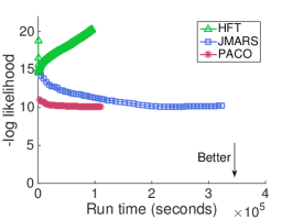
(a) Amazon fine foods

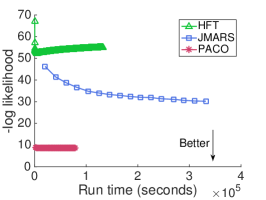
(b) RateBeer

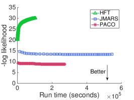
(c) Yelp

Figure 1: Negative log likelihood: PACO better jointly predicts ratings and reviews than state-of-the-art JMARS [7] and HFT [17] on Amazon fine foods, Yelp and RateBeer datasets. The joint predictive power is captured by the normalized negative log likelihood as described in (21). Lower is better.

With this approach we make a number of contributions:

• We design a Poisson additive co-clustering model for backfitting word counts in documents. We combine this with ACCAMS [3] to learn a joint Bayesian model of reviews and ratings, with the ability to now interpret our model.

• We describe a new, efficient technique for sampling from a sum of Poisson random variables to facilitate efficient inference. It relies on treating discrete counts as “residuals,” similar to an additive regression model.

• We give empirical evidence across multiple datasets that PACO has better prediction accuracy for ratings than competing methods, such as HFT [17] and JMARS [7]. Additionally, our method predicts text reviews better than HFT, and achieves nearly as high quality review prediction as JMARS, while being far faster and simpler. As seen in Figure 1, PACO outperforms both competing models in jointly predicting ratings and reviews.

In summary, we propose a simple and novel model and sampler, capable of characterizing user and item attributes very concisely, while providing excellent accuracy and perplexity.

2 Related Work

Our model, while significantly different from previous approaches, touches upon research from a variety of fields.

Collaborative Filtering

Collaborative filtering is a rich field of research. In particular, factorization models that learn a bilinear model of latent factors have proven to be effective for recommendation problems [13, 12]. A variety of papers have adapted frequentist intuition on factorization to Bayesian models [22, 19, 25, 4]. Of particular note are Probabilistic Matrix Factorization (PMF) and Bayesian Probabilistic Matrix Factorization (BPMF) [22], which we will compare to later. Recently, ACCAMS [3] took a drastically different approach from classic bilinear models. It uses an additive model of co-clusterings to approximate matrices succinctly. While the resulting model is simple and small, its prediction quality is as good as more complex factorization models.

A separate line of research in recommender systems has focused on using side information to improve prediction quality. This is particularly important when parts of the data are extremely sparse, i.e. the cold start problem. Content-based filtering is a popular approach to alleviate this problem. Regression based latent factor models (RLFM) [1] address cold-start problem by utilizing user and item features. Cold-start users and items are able to share statistical strength with other users and items through similarity in features space. fLDA [2] uses text associated with items and user features to regularize item and user factors, but does not make use of review text.

More recently, there has been a growing line of research on using Poisson distributions in matrix factorization models [8, 23, 5]. This work shows the exciting potential uses of Poisson distributions for understanding matrix data. However, all of these models are left with limited interpretability since they, too, rely on bilinear models. Additionally, all of these models rely on variational inference to learn the models. Our work provides the building blocks for using Poisson distributions in a wide array of additive clustering applications and is the first work to learn a model of this sort through Gibbs sampling rather than variational inference.

Review Mining and Modeling

Modeling online reviews has long been a focus of the data mining, machine learning and natural language processing communities [9]. Significant research has focused on understanding and finding patterns in online reviews [6]. More closely related to our work, a variety of papers model aspects and sentiments of reviews [15, 14, 10, 11]. For example, [11] considers hierarchical structures in aspects and sentiments. However, in these works ratings are not considered jointly.

Multimodal Models

Recently, there is increasing attention in jointly modeling review text and ratings. Collaborative topic regression (CTR) [28] combines topic modeling and collaborative filtering to recommend scientific articles. HFT [17] jointly models both ratings and reviews by designing link function to connect each topic dimension to a latent factor, demonstrating improvements in rating prediction. RMR [16] relaxes the hard link between topic and latent factor dimension for interpretable topics. [31] considers review texts with hidden user communities and item groups relationship. JMARS [7] jointly models aspects, sentiments, items, reviews, and ratings based on insights in review structure.

A related line of work models multi-aspect ratings [18, 27]. However, these works often rely on availability of aspect-specific ratings, which are often not available. In contrast, our models learns sentiments in different aspects without requiring multi-aspect ratings.

Additive Clustering

Our model, built on additive co-clustering, takes a different approach from classic collaborative filtering literature. Our approach is conceptually similar to older literature from psychology on additive clustering [24, 26, 20]. ADCLUS [24] argues that similarity between objects should be based on similarity on a subset of discrete properties. This perspective reinforces our belief that additive co-clustering is a good fit for user behavior modeling.

From a computational perspective, ACCAMS [3], described above, focuses on an additive co-clustering model of Gaussian distributions and describes a collapsed sampler for efficient learning. [21] uses a sum of clusters within a logistic function for modeling binary data but has difficulty scaling. Here we demonstrate that we can successfully scale learning a sum of clusters within a Poisson distribution.

Symbol	Definition
$N,M$	Number of rows (users) and columns (items)
$\mathbf{R}$	Data matrix $\in\mathbb{R}^{N\times M}$ (with missing values)
$\mathcal{I}$	Indicator matrix $\in\{0,1\}^{N\times M}$ for $\mathbf{R}$
$S$	Number of stencils
$k_{n}^{(\ell)},k_{m}^{(\ell)}$	Number of user and item clusters in stencil $\ell$
$\mathbf{T}^{(\ell)}$	Matrix $\in\mathbb{R}^{k_{n}^{{(\ell)}}\times k_{m}^{{(\ell)}}}$ for stencil $\ell$
$\mathbf{c}^{(\ell)}$	Vector of user assignments $\in\{1,\ldots,k_{n}^{(\ell)}\}^{N}$
$\mathbf{d}^{(\ell)}$	Vector of item assignments $\in\{1,\ldots,k_{m}^{(\ell)}\}^{M}$
$\mathcal{S}(\mathbf{T},\mathbf{c},\mathbf{d})$	$\in\mathbb{R}^{N\times M}$ defined by $\mathcal{S}(\mathbf{T},\mathbf{c},\mathbf{d})_{u,m}=\mathbf{T}_{\mathbf{c}_{u},\mathbf{d}_{m}}$
$\mathcal{W}$	Set of all words used in the reviews
$n_{u,m,x}$	Count for word $x$ in review $(u,m)$
$\mu^{(i)}_{x}$	Rate of Poisson in language model $i$ for word $x$
$\mathcal{L}_{u,m}$	Set of language models used for review $(u,m)$

Table 1: Symbols used throughout this paper.

3 Additive Co-Clustering

We begin by giving a general overview of additive co-clustering in order to gain familiarity with the notation and problem. A full list of the symbols used can be found in Table 1. We will use bold uppercase letters to denote matrices, bold lower case letters to denote vectors, and non-bold letters for scalars. To index into a matrix or vector we will use subscripts, e.g. $\mathbf{R}_{u,m}$ refers to the value in row $u$ and column $m$ of $\mathbf{R}$; we will use “:” to select an entire row or column in a matrix when necessary. Superscripts are often used to denote different instances of the object.

Our goal is to jointly model documents and review scores. For the sake of completeness, we briefly review the formulation of additive co-clustering for Gaussian data, as described in ACCAMS. We focus on the problem of matrix approximation, where we have a real valued (often sparse) matrix, where we observe a small percentage of the entries in the matrix and our goal is to predict the missing values. To be precise, we have a matrix $\mathbf{R}\in\mathbb{R}^{N\times M}$ with the set $\mathcal{I}$ of observed entries $(u,m)$. To predict the missing values, we would like to learn a model $\mathcal{M}$ with parameters $\theta$, such that the size of $\theta$ is small, $|\theta|\ll|\mathcal{I}|$, and $\mathcal{M}(\theta)$ approximates $\mathbf{R}$ well:

$$\operatorname*{\mathrm{minimize}}_{\theta}\sum_{(u,m)\in\mathcal{I}}(\mathbf{R}_{u,m}-\mathcal{M}(\theta)_{u,m})^{2}$$ (1)

The concept of a small model in the context of behavior modeling has typically been captured by low rank factorization of the rating matrix. We consider the generalization of this concept, defining a small model by the number of bits required to store it.

Key to our model is the notion of a stencil, an extremely easy way to represent a block-wise constant rank-$k$ matrix. A stencil $\mathbf{T}$ assigns each row $u$, typically a user, to a row cluster $a$, each column, typically an item, to a column cluster $b$. The rating that user $u$ gives to item $m$ is thus predicted by the value $\mathbf{T}_{a,b}$. Formally:

Definition 1 (Stencil)

A stencil $\mathcal{S}\left(\mathbf{T},\mathbf{c},\mathbf{d}\right)$ is a block-wise constant matrix $\mathcal{S}\in\mathbb{R}^{N\times M}$ with the property that

$$\mathcal{S}\left(\mathbf{T},\mathbf{c},\mathbf{d}\right)_{u,m}=\mathbf{T}_{\mathbf{c}_{u},\mathbf{d}_{m}}\text{ for a template }\mathbf{T}\in\mathbb{R}^{k_{n}\times k_{m}}$$

and index vectors $\mathbf{c}\in\left\{1,\ldots,k_{n}\right\}^{N}$ and $\mathbf{d}\in\left\{1,\ldots,k_{m}\right\}^{M}$.

Therefore, our goal is to find a stencil $\mathcal{S}\left(\mathbf{T},\mathbf{c},\mathbf{d}\right)$ with a small approximation error $\mathbf{R}-\mathcal{S}\left(\mathbf{T},\mathbf{c},\mathbf{d}\right)$.

We observe that storing a stencil with small $k_{n},k_{m}$ is quite compact, with the cost in bits bounded by [3]:

$$\mathrm{Bits}(\{\mathbf{T},\mathbf{c},\mathbf{d}\})=N\log_{2}k_{n}+M\log_{2}k_{m}+32k_{n}k_{m}$$ (2)

Note that this bound is very loose, as it ignores any properties of the distribution of $\mathbf{c}$ and $\mathbf{d}$. That said, even the worst case bound is much tighter than what can be accomplished with inner product models. To improve the approximation accuracy without making the model size grow quickly, we can use multiple stencils in an additive fashion:

$$\operatorname*{\mathrm{minimize}}_{\left\{\mathbf{T}^{(\ell)},\mathbf{c}^{(\ell)},\mathbf{d}^{(\ell)}\right\}}\sum_{(u,m)\in\mathcal{I}}\left(\mathbf{R}_{u,m}-\sum_{\ell=1}^{S}\mathcal{S}\left(\mathbf{T}^{(\ell)},\mathbf{c}^{(\ell)},\mathbf{d}^{(\ell)}\right)_{u,m}\right)^{2}$$

That is, we would like to find an additive model of $S$ stencils that minimizes the approximation error to $\mathbf{R}$.

Unfortunately, finding linear combinations of co-clusterings is NP-hard. It is easy to see this by reducing co-clustering, which is NP-hard, to our problem by setting $S=1$. In [3], we showed how to solve this problem using a back fitting algorithm. To make the problem tractable, we assumed that user and item clusters in each stencil follow a Chinese restaurant process (CRP), and that the observed ratings are normally distributed across the mean of each co-cluster. Formally speaking, we have the following generative model [3]:

$$\mathbf{R}_{u,m} \sim\mathcal{N}\left(\sum_{\ell=1}^{S}\mathcal{S}\left(\mathbf{T}^{(\ell)},\mathbf{c}^{(\ell)},\mathbf{d}^{(\ell)}\right)_{u,m},\sigma^{2}\right)$$ (3)

$$\mathbf{c}^{(\ell)},\mathbf{d}^{(\ell)} \sim\mathrm{CRP}(\delta)\text{ for all }{(\ell)}$$ (4)

$$\mathbf{T}^{(\ell)}_{c,d} \sim\mathcal{N}(0,\sigma^{2}_{(\ell)})$$ (5)

The benefit of this model is that conditioned on all stencils but one, the problem of inferring $\mathbf{T}^{(\ell)}$ becomes one of inferring Gaussian random variables for the rating (i.e. $\mathbf{T}^{(\ell)}_{c,d}$ ). Likewise, inferring $\mathbf{c}^{(\ell)}$ and $\mathbf{d}^{(\ell)}$ is a straightforward clustering problem. Thus, the backfitting algorithm sweeps through all stencils, one at a time, estimating the stencil’s users and items cluster assignments in addition to the co-clusters ratings. We have shown in [3], that fitting stencil $\ell$ while fixing other stencils, is equivalent to fitting the residual error between the observed ratings and the current estimate using all stencils but stencil $\ell$. This algorithm converges with guarantees as shown in [3].

4 Poisson Additive Co-Clustering

Figure 2: The generative model for PACO to predict both ratings $\mathbf{R}$ and review text $n$. (Note, for the sake of space we simplify the model slightly by not explicitly separating the different language models associated with each stencil.)

While ACCAMS [3] explains the ratings matrix well, it does not utilize the reviews associated with those ratings. In this section we introduce PACO, a Poisson Additive co-clustering model that jointly model text and reviews. PACO builds on the idea of stencils introduced in ACCAMS. Each stencil $\mathbf{T}$ assigns each user $u$ to a cluster say $a$ and each item $m$ to a cluster say $b$. Given the block (i.e. co-cluster) denoted by $\mathbf{T}_{a,b}$, we design a model to jointly generates both the rating user $u$ gives to item $m$ as well as the review she wrote for this item. We endow each block with a Gaussian distribution that model the mean rating associated with cluster $a$ and $b$. The question now is: how can we parametrize the text model of block $(a,b)$?

4.1 Modeling Reviews using an Additive Poisson Model

A standard approach in the text mining literature is to model reviews using a multinomial distribution; however, in PACO, as in ACCAMS, we want to combine multiple stencils to enhance the model. While it is easy to define an additive model over review scores, it is nontrivial to accomplish this using multinomial distributions for reviews. Quite obviously, if $p$ and $q$ are multinomial probability distributions, then $p+q$ is no longer in the probability simplex. Instead, the transform is given by $(p+q)/\left\|p+q\right\|_{1}$, thus making updates highly nontrivial, since additivity of the model is lost, which means that we would need to update the entire language model whenever even just a single stencil changes. This would make a backfitting algorithm very expensive.

Rather, we introduce a novel approach to modeling using the Poisson distribution. In a nutshell, we exploit the fact that the Poisson distribution is closed under addition, i.e. for

$$a\sim\mathrm{Poi}(\lambda)\text{ and }b\sim\mathrm{Poi}(\gamma)\text{ we have }a+b\sim\mathrm{Poi}(\lambda+\gamma)$$

where $\lambda$ and $\gamma$ denote the rates of each of the random variables, i.e. $\mathbf{E}[a]=\lambda$ and $\mathbf{E}[b]=\gamma$.

For each user and item pair $(u,m)$ pair we let $n_{u,m,x}$ denote the count for word $x$ in the review. We now design an additive model for each review. The idea is that the distribution over each word is given by a sum over Poisson random variables with rates $\mu_{\mathbf{c}_{u}^{(\ell)},\mathbf{d}_{m}^{(\ell)},x}^{(\ell)}$ for each word $x$ across all stencils. The benefit of this approach is that we no longer need to ensure normalization. We will detail the generative model in the following subsection.

4.2 The Joint Generative Model

Now we are ready to present the full model. To design a joint model we face an important challenge: we need to assess whether to perform good recommendation or whether we strive to optimize for good perplexity. In the former case, it is undesirable if the reviews carry the majority of the statistical weight. Hence it is worthwhile to normalize the reviews by their length. This technique is common in NLP literature [30, 29]. This yields the following joint objective:

$$\operatorname*{\mathrm{minimize}}_{\left\{\mathbf{T}^{(\ell)},\mathbf{c}^{(\ell)},\mathbf{d}^{(\ell)},\lambda\right\}} \sum_{(u,m)\in\mathcal{I}}\left(\mathbf{R}_{u,m}-\sum_{\ell=1}^{S}\mathcal{S}\left(\mathbf{T}^{(\ell)},\mathbf{c}^{(\ell)},\mathbf{d}^{(\ell)}\right)_{u,m}\right)^{2}$$

$$+\sum_{(u,m)\in\mathcal{I}}\frac{1}{|n_{u,m}|_{1}}\sum_{x\in\mathcal{W}}\log\mathrm{Poi}(\lambda_{u,m,x})$$

where

$$\lambda_{u,m} =\mu^{(0)}\!+\!\mu^{(m)}\!+\!\left[\sum_{\ell=1}^{S}\mu_{\mathbf{c}_{u}^{(\ell)},\mathbf{d}_{m}^{(\ell)}}^{(\ell)}\!+\!\mu_{\mathbf{d}_{m}^{(\ell)}}^{(m,\ell)}\!+\!\mu_{\mathbf{c}_{u}^{(\ell)}}^{(u,\ell)}\right]$$ (6)

Our goal is to learn a set of stencils whose summation minimizes the prediction error on ratings and maximizes the likelihood of generating the text. To model review text, we allow each stencil to have three language models: a stencil-specific user language model $\mu_{\mathbf{c}_{u}^{(\ell)}}^{(\ell)}$, a stencil-specific item language model $\mu_{\mathbf{d}_{m}^{(\ell)}}^{(m,\ell)}$, and block language model, $\mu_{\mathbf{c}_{u}^{(\ell)},\mathbf{d}_{m}^{(\ell)}}^{(\ell)}$. The block language model captures the stencil-specific interaction between the item and the user. In addition, we add a global item language model, $\mu^{(m)}$, and a global background language model, $\mu^{(0)}$. The text of the review is modeled as a combination of these Poisson language models.

Minimizing the aforementioned objective function is approximately equivalent to maximizing the log-likelihood of the graphical model in Figure 2. The generative process proceeds as follows:

$$\mathbf{R}_{u,m} \sim\mathcal{N}\left(\sum_{\ell=1}^{S}\mathcal{S}\left(\mathbf{T}^{(\ell)},\mathbf{c}^{(\ell)},\mathbf{d}^{(\ell)}\right)_{u,m},\sigma^{2}\right)$$ (7)

$$\mathbf{c}^{(\ell)},\mathbf{d}^{(\ell)} \sim\mathrm{CRP}(\delta)\text{ for all }{(\ell)}$$ (8)

$$\mathbf{T}^{(\ell)}_{c,d} \sim\mathcal{N}(0,\sigma^{2}_{(\ell)})$$ (9)

$$n_{u,m,x} \sim{\mathrm{Poi}}\left(\lambda_{u,m,x}\right)$$ (10)

$$\mu^{(*)}_{x} \sim{\rm Gamma}(\alpha,\beta)$$ (11)

where $\mathbf{c}_{u}^{(\ell)},\mathbf{d}_{m}^{(\ell)}$ is the cluster $(u,m)$ assigned to in stencil $\ell$. In essence, we model user and item clusters inside each stencil using a Chinese restaurant process (CRP). Ratings are modeled similar to ACCAMS while (6), (10) and (11) contain the additional text modeling aspects of our model. To avoid overfitting, we use conjugate Gamma prior for all the vectors $\mu$:

$$P(\mu_{x})=\frac{\beta^{\alpha}}{\Gamma(\alpha)}\mu_{x}^{\alpha-1}e^{-\beta\mu_{x}}$$

Since the mode of the Gamma distribution is $\frac{\alpha-1}{\beta}$, a very large $\beta$ should ensure that only a small amount of data is blamed. Given this model, we now consider the challenge of learning the parameters in practice.

5 The Sampling Algorithm

The goal of inference is to learn a posterior distribution over stencils’ parameters which are: user and item cluster assignments, stencil ratings of each block, and the multiple language models. To do this, we use Gibbs sampling.

Jointly sampling text and rating adds significant complications over just sampling ratings data and requires a novel sampling technique. In particular, our sampler offers (1) a new novel technique to learn the sum of Poisson rates $\mu$ and (2) an efficient method for sampling cluster assignments based on both the text model and ratings model. We describe each of these challenges and solutions below in Section 5.1, followed by the complete learner shown in Algorithm 1, which combines the new, novel Poisson sampler and ACCAMS’s sampler for Gaussian rating data.

5.1 Sampling a Sum of Poisson Distributions

The Gamma distribution is conjugate to the Poisson distribution, typically allowing for an easy sampling of the Poisson’s rate $\lambda$ from the Gamma distribution. However, in this case we have a sum of Poisson distributions and we would like to sample the rate of each of these distributions.

To make this tractable, we create a multinomial the from rates of the involved Poisson distributions and sample form this multinomial the fraction of counts coming from each Poisson distributions. To be precise, for a particular $n_{u,m,x}$ we have $\lambda_{u,m,x}=\sum_{i\in\mathcal{L}_{u,m}}\mu^{(i)}_{x}$, where $\mathcal{L}_{u,m}$ is the set of Poisson distributions from which words in $(u,m)$ are sampled. We define:

$$\left\{\mu^{(*)}_{u,m,x}\right\}:=\left\{\mu_{x}^{(i)}\right\}_{\forall i\in\mathcal{L}_{u,m}}\text{ and }\left\{\hat{n}_{u,m,x}\right\}:=\left\{\hat{n}_{u,m,x}^{(i)}\right\}_{\forall i\in\mathcal{L}_{u,m}}$$ (12)

We can therefore sample $\left\{\hat{n}_{u,m,x}\right\}$ by

$$\left\{\hat{n}_{u,m,x}\right\} \sim{\rm Multi}\left(\frac{\left\{\mu^{(*)}_{u,m,x}\right\}}{\lambda_{u,m,x}},n_{u,m,x}\right).$$ (13)

The result is $n_{u,m,x}=\sum_{i\in\mathcal{L}_{u,m}}\hat{n}_{x}^{(i)}$. That is, if we observe $n_{u,m,x}$ occurrences of word $x$ in review $(u,m)$, we break this count to a set of $\hat{n}_{x}^{(i)}$ counts, each of which are credited to the corresponding Poisson distribution $i$, where $i$ indexes over the set of involved Poisson distributions. For example, if the word “delicious” is used three times in a review, we may consider one use of the word to be “from” the base language model and two uses of the word to be “from” the item-specific language model.

By sampling these count allocations, we can now tractably sample our Poisson rates and later our cluster assignments. To sample a particular $\mu^{(i)}_{x}$, we consider $\mathcal{R}_{i}$, the set of reviews $(u,m)$ partially sampled form a Poisson distribution with rate $\mu^{(i)}$. Therefore, we can sample $\mu^{(i)}_{x}$ by:

$$\mu_{x}^{(i)} \sim\Gamma\left(\alpha^{(i)},\beta^{(i)}\right)\!\prod_{(u,m)\in\mathcal{R}_{i}}\!{\mathrm{Poi}}\left(\left.\hat{n}_{u,m,x}^{(i)}\right|\mu_{x}^{(i)}\right)$$ (14)

$$\sim\Gamma\!\left(\alpha^{(i)}\!+\!\!\sum_{(u,m)\in\mathcal{R}_{i}}\!\hat{n}_{u,m,x}^{(i)},\beta^{(i)}+\left|\mathcal{R}_{i}\right|\right)$$ (15)

This is trivially parallelized across all words in a particular language model $\mu$, which we will expand on later.

5.2 Sampling Cluster Assignments

For each stencil, we need to sample the cluster assignment for each user and item. To do this for users, we need to calculate the posterior distribution $p(\mathbf{c}_{u}^{(\ell)}=a|{\rm rest})$ for each cluster $a$. This probability is composed of three main terms: (1) the CRP prior, (2) the likelihood of the user ratings and (3) the likelihood of the user review texts. This can be written as

$$p(\mathbf{c}_{u}^{(\ell)}=a|{\rm rest})\propto{\rm CRP}(a)\prod_{(u,m)\in\mathcal{R}_{u}}p(\mathbf{R}_{u,m}|{\rm rest})\prod_{x}p(n_{u,m,x}|{\rm rest})$$

where $\mathcal{R}_{u}$ denotes the set of reviews from user $u$. This probability in log-space (incorporating review normalization) becomes:

$$\log p(\mathbf{c}_{u}^{(\ell)}=a|{\rm rest})\propto\log\left({\rm CRP}(a)\right)+\sum_{(u,m)\in\mathcal{R}_{u}}\log p(\mathbf{R}_{u,m}|{\rm rest})+\frac{1}{|n_{u,m}|}\sum_{x}\log p(n_{u,m,x}|{\rm rest})$$ (16)

The details for calculating the CRP term and rating terms can be found in [3]. Here, we focus on how to efficiently calculate the term that corresponds to probability of the reviews.

To calculate the probability of the text, we in fact focus on the $\hat{n}_{u,m,x}$ rather than $n_{u,m,x}$. Specifically, when sampling the user cluster assignment, we must calculate on

$$\Delta_{u,a} :=\sum_{(u,m)\in\mathcal{R}_{u}}\sum_{x}\log\;{\mathrm{Poi}}\left(\left.\hat{n}^{(\ell)}_{u,m,x}\right|\mu^{(\ell)}_{a,\mathbf{d}^{(\ell)}_{m},x}\right)+\log\;{\mathrm{Poi}}\left(\left.\hat{n}^{(u,\ell)}_{u,m,x}\right|\mu^{(u,\ell)}_{a,x}\right)$$

$$=\sum_{(u,m)\in\mathcal{R}_{u}}\sum_{x}\hat{n}^{(\ell)}_{u,m,x}\log\left[\mu^{(\ell)}_{a,\mathbf{d}^{(\ell)}_{m},x}\right]-\mu^{(\ell)}_{a,\mathbf{d}^{(\ell)}_{m},x}+\hat{n}^{(u,\ell)}_{u,m,x}\log\left[\mu^{(u,\ell)}_{a,x}\right]-\mu^{(u,\ell)}_{a,x}$$ (17)

For $k$ clusters, to naively calculate $\Delta_{u,a}$ for each user would require $O(k|\mathcal{W}|)$ logarithm evaluations, which are significantly slower than the other simple addition and multiplication operations. However, we can accelerate this significantly. Define the following terms:

$$\tilde{\mu}_{a,b}^{(\ell)} =\sum_{x}\mu_{a,b,x}^{(\ell)} \tilde{\mu}_{a}^{(u,\ell)} =\sum_{x}\mu_{a,x}^{(\ell)}$$ and

$$\eta_{u,b} =\sum_{\begin{subarray}{c}m|\mathbf{d}^{(\ell)}_{m}=b,\\ (u,m)\in\mathcal{R}_{u}\end{subarray}}1 \hat{\eta}^{(\ell)}_{u,b} =\sum_{\begin{subarray}{c}m|\mathbf{d}^{(\ell)}_{m}=b,\\ (u,m)\in\mathcal{R}_{u}\end{subarray}}\hat{n}^{(\ell)}_{u,m} \hat{\eta}^{(u,\ell)}_{u} =\sum_{(u,m)\in\mathcal{R}_{u}}\hat{n}^{(u,\ell)}_{u,m}$$ and and

All of these terms can be pre-calculated and cached for sampling all cluster assignments for stencil $\ell$. Now we can rearrange the terms of (17) to achieve the following simplified equation:

$$\Delta_{u,a} =-\sum_{b=1}^{k}\eta_{u,b}\left(\tilde{\mu}_{a,b}^{(\ell)}+\tilde{\mu}_{a}^{(u,\ell)}\right)+\left\langle\hat{\eta}^{(\ell)}_{u,b},\log\mu^{(\ell)}_{a,b}\right\rangle+\left\langle\hat{\eta}^{(u,\ell)}_{u},\log\mu^{(u,\ell)}_{a}\right\rangle$$ (18)

With this formulation we can cache the logarithm of each $\mu_{a,b,x}$ and $\mu_{a,x}$ and reuse them for sampling cluster assignment of each user. As such, we only need to take one pass over the original data and thus minimize the number of logarithm computations in each iteration. Sampling item cluster assignments can be done by an analogous sampler. We will show in Section 5.3 that this approach results in a fast sampling procedure.

Now we are ready to describe our full Gibbs sampling algorithm. For each stencil, we first update the rating model (see [3] for details) and then update the text model using aforementioned techniques: Specifically, we resample $\hat{n}$ following (13), and then resample the stencil’s $\mu$ terms (i.e. the Poisson language models associated with that stencil) based on $\hat{n}$, following (15). Finally, we update the cluster assignments for a given stencil following (16). The full procedure is given in Algorithm 1.

Algorithm 1 PACO Sampler

  Run K-Means ACCAMS for initial cluster assignments.

  Initialize all $\mu^{(i)}$ to a vector $\mathbf{1}$

  while not converged  do

     Resample $\{\hat{n}_{u,m,x}\}$ for all $u,m,x$ by (13)

     Sample $\mu^{(0)}$ by (15)

     for Stencil $\ell=1,\dots,S$ do

        Update predicted ratings as described in [3]

        if Not first iteration then

           Resample $\{\hat{n}_{u,m,x}\}$ for all $u,m,x$ by (13)

        end if

        Sample $\mu^{(\ell)},\mu^{(m,\ell)},\mu^{(u,\ell)}$ by (15)

        Sample $\mathbf{c}_{u}^{(\ell)}$ by (16)

        Sample $\mathbf{d}_{m}^{(\ell)}$ analogous to (16)

     end for

     Sample $\mu^{(m)}$ by (15)

  end while

5.3 Implementation

The sampler is written in C++11. The implementation is very efficient and uses the following techniques. Sampling $\left\{\hat{n}_{u,m,x}\right\}$ is embarrassingly parallelizable across reviews. With $\mu$ fixed, this involves simply parallel sampling from the re-parametrized multinomials. Sampling the Poisson rate $\mu$ is also embarrassingly parallelizable across $\mu$ and across words. We use C++11 implementation of Gamma sampler. The review likelihood can be efficiently calculated when sampling user/item cluster assignments. With $\tilde{\mu}_{a,b}^{(\ell)}$, $\tilde{\mu}_{a}^{(u,\ell)}$, $\log(\mu_{a,b,x}^{(\ell)})$ and $\log(\mu_{a,x}^{(u,\ell)})$ cached, the review likelihood can be calculated with one pass over non-zero words. Again, this can be parallelized across users/items.

Speed: We generally found the above optimizations to make our sampler sufficiently fast for the large datasets we tested on. On the Amazon fine foods dataset described below, sampling all cluster assignments for ons stencil takes 3.66 seconds on average, sampling all $\hat{n}$ for half million reviews takes 45 seconds, and sampling all $\mu$ for one stencil takes less than one second on a single machine.

6 Experiments

We now test our model in a variety of settings both to understand how it models different types of data and to demonstrate its performance against similar, recent models.

6.1 Experimental Setup

Datasets

To test our model, we select four datasets about movies, beer, businesses, and food. All four datasets come from different websites and communities, thus capturing different styles and patterns of online ratings and reviews. In all of these datasets, one observed (user,item) pair is associated with one rating and one review. We randomly select 80% of data as training set and 20% as testing set while making sure every user and item in the testing set has at least one example in training set. Infrequent words, standard stop words and words shorter than 3 characters are removed. We rescale ratings to the same range during training and center all ratings based on the global average in the dataset. The resulting datasets are summarized in Table 2.

Dataset	Yelp	Food	RateBeer	IMDb
# items	60,785	74,257	110,369	117,240
# users	366,715	256,055	29,265	452,627
# observations	1,569,264	568,447	2,924,163	1,462,124
# unigrams	9,055	9,088	8,962	9,182
avg. review length	45.20	31.55	28.57	88.30

Table 2: Four datasets used in experiments. Infrequent words, standard stop words and words shorter than 3 characters are removed during pruning.

Metrics

To evaluate our review model, we examine its ability to predict held-out testing ratings and reviews.

RMSE: When comparing predictions of held-out ratings, we use the root mean squared error (RMSE) to compare prediction quality. For PACO, we average predictions over many samples from the posterior, as is customary in evaluating sampling-based algorithms.

Perplexity: When evaluating the ability to predict held-out reviews, we compare perplexity of review text with other models. In order to have a comparable definition of perplexity, following the usual intuition as the average number of bits necessary to encode a particular word of review, we transform our model as follows. We use $\lambda_{u,m}$ as defined in (6) as the vector of expected counts for each word to be in a review from user $u$ about item $m$. We transform this vector to a multinomial with probabilities $\theta_{u,m}$ where

$$\theta_{u,m,x}=\frac{\lambda_{u,m,x}}{\sum_{x}\lambda_{u,m,x}}$$ (19)

Note that when we average over multiple samples from the posterior, we average $\lambda_{u,m}$ over those samples and use the averaged rate of the Poisson in (19). With this multinomial, we calculate perplexity of testing set $D_{test}$ as

$$-\log{\rm PPX}(D_{test})=\frac{1}{N_{w}}\sum_{(u,m)\in D_{test}}\sum_{x}n_{u,m,x}\log\theta_{u,m,x}$$ (20)

where $N_{w}$ is the total number of words in held-out testing reviews. Note that this now views our Poisson distributions in their expected state, but makes our quite different model more easily comparable to previous techniques.

Joint Negative Log-Likelihood: To evaluate the models jointly in terms of both rating and text prediction, we compare the joint negative log-likelihood. Per-review joint negative log-likelihood is defined as

$$-\log({\rm PPX})\!-\!\frac{1}{\left|D_{test}\right|}\!\sum_{(u,m)\in D_{test}}\!\log\left(\mathcal{N}\left(\mathbf{R}_{u,m}|\hat{\mathbf{R}}_{u,m},\sigma^{2}\right)\right)$$ (21)

The text likelihood is normalized by number of words in review to equally weight the importance of predicting ratings and text. $\sigma$ is taken from the training of each model.

Baseline methods

We compare PACO with the following models:

PMF

Probabilistic matrix factorization (PMF) [19] factorizes ratings into latent factors. It is simple in structure but usually effective. A number of latent factors with Rank $\in\left\{10,20\right\}$ were tested.

BPMF

Bayesian probabilistic matrix factorization (BPMF) [22] takes a more directly Bayesian approach to matrix factorization. Number of latent factors Rank $\in\left\{10,20\right\}$ were tested.${}^{\ref{bpmf_source}}$

HFT

Hidden factors with topics (HFT) [17] is one of the state-of-the-art models that jointly model ratings and reviews. It builds connection between topic distribution of reviews and latent factors. It shows significant improvement on rating prediction over traditional latent factor models on a variety of datasets. We use the implementation from the authors’ website and run it with parameters recommended in the original paper.

JMARS

[7] is another state-of-the-art model in joint-review-rating modeling. It explicitly models aspects, sentiments, ratings and reviews and provides interpretable and accurate recommendation. Similarly, parameters recommended in the original paper is used.

Note, PMF and BPMF only optimize for prediction accuracy on ratings, thus only focusing on half of the problem we are attacking. However, we include them for completeness.

We test PACO with different priors and combinations of language models, where we include per-block language models, per-user cluster language models, or per-item cluster language models, or some combination thereof. For all datasets we use these joint text and rating stencils for the first $S_{0}$ stencils and then a series of rating-only stencils. All results from PACO are reported based for the best RMSE.

6.2 Quantitative evaluation

6.2.1 Joint Predictive Ability

We compare the ability of PACO to predict jointly reviews and ratings against that of HFT and JMARS. In particular, we track the joint negative log-likelihood by runtime in Figure 1 and give the detailed numbers for best results in Table 3. We observe that PACO converges rapidly and has superior performance to both competitors on all four datasets. We note that while HFT very quickly reaches reasonable accuracy on both text and ratings, it very quickly overfits its model of ratings, causing the surprising curve in Figure 1. However, results reported in Table 3 for all models are based on the best RMSE so as to prevent skew from overfitting. While we clearly offer high quality joint performance, we now look more closely at our prediction accuracy for ratings and for text separately.

	HFT	JMARS	PACO
RateBeer	52.3546	30.2174	8.5994
Yelp	20.1377	13.3171	8.9300
Amazon fine foods	14.5827	10.1129	10.0904
IMDb	57.4515	33.7715	31.2567

Table 3: Joint prediction accuracy for text reviews and ratings, as given by joint negative log-likelihood (21), for all datasets. Lower is better.

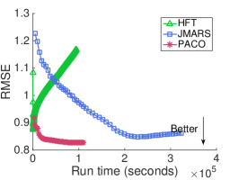
(a) Amazon fine foods

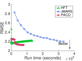
(b) RateBeer

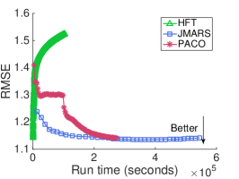
(c) Yelp

Figure 3: Rating prediction accuracy (RMSE) compared by runtime to other joint modeling systems$.^{4}$

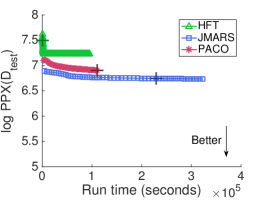
(a) Amazon fine foods

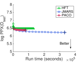
(b) RateBeer

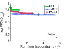
(c) Yelp

Figure 4: Log perplexity of review text predictions on three datasets. Plus sign markers indicate the values corresponding to the best RMSE. (Lower is better.)

6.2.2 Rating prediction

We evaluate performance of rating prediction based on RMSE. Figure 4 shows RMSE over runtime, and Table 4 presents detailed results. A number of interesting patterns emerge in these results. In Figure 4, we observe more clearly that HFT converges extremely quickly before overfitting, but again results reported in Table 4 are from best RMSE before overfitting. For PACO we observe reasonable RMSE before burn-in and then quickly improved RMSE after burn-in. Finally we observe that JMARS is generally slower to converge.

In Table 4 we observe that PACO has superior performance to both HFT and JMARS on RateBeer, Amazon fine foods, and IMDb; JMARS performs slightly better on Yelp. While PACO generally outperforms the competing joint models, in these experiments it achieves slightly worse accuracy than BPMF. Here we observe a general trade-off between size and performance. As discussed in [3], using a sum of co-clusterings is far more succinct than bilinear models like BPMF. As a result, the ratings model in PACO is far smaller than that of BPMF, while we consistently achieve nearly as high of an accuracy.

	PMF	BPMF	HFT	JMARS	PACO
RateBeer	2.1944	2.1164	2.1552	2.1675	2.1273
Yelp	1.2649	1.1346	1.1408	1.1347	1.1407
Amazon fine foods	0.8752	0.8193	0.8809	0.8486	0.8292
IMDb	2.5274	2.1622	2.2328	2.2947	2.1877

Table 4: Rating prediction accuracy (RMSE) across all four datasets. We observe that PACO generally outperforms the other joint learning models (HFT and JMARS) as well as PMF.

6.2.3 Review Text Prediction

The second component of the predictive ability of our model is predicting review text, as measured by perplexity. We give the perplexity over runtime in Figure 4. We observe an apparent trade-off in perplexity for speed, simplicity and accuracy in rating prediction. PACO is efficient and outperforms HFT on all datasets. Note, in [17], HFT is described to primarily use text to improve rating predictions and not for predicting review. JMARS gives slightly better perplexity at the cost of significantly more complex model. Precise perplexity of HFT, JMARS, and PACO are given in Table 5. Since our primary goal is recommendation, the perplexity reported correspond to the points that obtain the best RMSE.

	HFT	JMARS	PACO
RateBeer	6.4891	6.2098	6.3779
Yelp	7.7031	7.1112	7.2223
Amazon fine foods	7.5015	6.7450	6.8759
IMDb	8.1747	7.4610	7.5540

Table 5: Perplexity on all four datasets. The perplexity values reported here correspond to the points that obtain the best RMSE.

6.2.4 Cold-start

For the sake of thoroughness, we looked at where does our joint model excel at rating prediction over the rating-only PMF model. We generally found PACO to help alleviate cold-start challenges. We show improvement in RMSE over PMF for items and users with different number of training examples in Figure 6 and 6. We observe that for items with fewer observed ratings we achieve a greater improvement in rating prediction accuracy. This suggests that PACO is able to extract rich information from reviews and provide benefits especially when items have scarce signals. For users with few ratings, we can see similar trends except for Amazon fine foods. One hypothesis is that the quality of food is less subjective than movies or beers. It is thus harder to learn user preference from the review in this case.

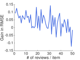
(a) Amazon fine foods

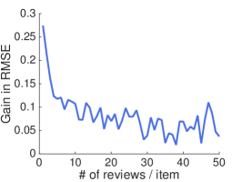
(b) RateBeer

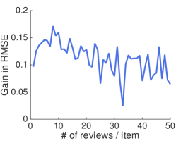
(c) Yelp

Figure 5: Gain of PACO over PMF in RMSE demonstrates the benefits for items with few observed ratings.

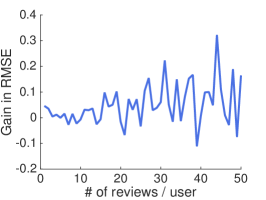
(a) Amazon fine foods

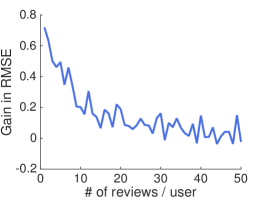
(b) RateBeer

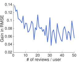
(c) Yelp

Figure 6: Gain of PACO over PMF in RMSE demonstrates the benefits for users with few observed ratings.

6.3 Interpretability

In addition to quantitatively evaluating our method, we also want to empirically demonstrate that the patterns surfaced and review predictions would be useful to the human eye. However, because reviews from each dataset follow very different patterns, we expect PACO to model them differently. In this effort, we analyzed our learned models to understand which parts of the models were effective in understanding each of these datasets.

Sentiment word extraction: We first checked to make sure that blocks in our co-clustering that had high rating predictions found appropriately positive or negative words. In Table 6 we present the top words in the highest-rating block and lowest-rating block in the first stencil for each dataset. We can see in general, in that high-rating blocks, there are more positive sentiment words, and in lower-rating blocks, more negative words. This is less clear in the RateBeer and Amazon fine foods datasets where reviews more strongly focus on describing the item. However, we still note the strong association with “good” for a positive rating and in some cases “bad” for a negative rating.

Dataset	Rating	Words
IMDb	0.022	great, love, movies, story, life, watch, time, people, character, characters, best, films, scene, watching
	-0.018	bad, good, plot, like, worst, money, waste, acting, script, movies, minutes, horrible, boring, thought
Fine foods	0.024	good, love, great, like, product, amazon, store, time, find, eat, price, years, buy, coffee, taste, stores
	-0.048	like, buy, taste, time, product, bought, purchased, good, pretty, thought, reviews, smell, purchase
Yelp	0.51	highly, recommend, professional, amazing, job, customer, work, best, appointment, staff, great, needed
	-0.76	told, manager, customer, called, call, rude, asked, horrible, worst, phone, minutes, order, money, hotel
RateBeer	0.15	nice, pours, hops, flavor, hop, citrus, color, taste, finish, tap, good, sweet, bitterness, white, malt, light
	-0.22	taste, bad, beer, like, color, good, decent, weak, drink, pours, beers, boring, special, watery, dont

Table 6: Blocks predict words matching the sentiment of the predicted rating.

Item-specific words: In Table 7, top item-specific words associated with some popular items are presented. In general these words provide basic descriptions unique to that particular item. We do observe some overfitting in cases where there are fewer reviews, but generally the item-specific language model improves predictive performance.

Item	Item-specific words
The Dark Knight	batman, joker, dark, ledger, knight, heath, nolan, best, performance, bale
Silent Hill	game, silent, hill, games, horror, video, rose, town, like, played, plot, scary
Canned Kitten Chicken Liver Food	food, time, kittens, kitty, liver, cats, feral, white, plan, female, guys, kitten
Low Fat Clusters and Flakes Cereal Raisin Bran	cereal, sugar, fat, wheat, calories, color, barley, raisins, ingredients, listed
Luxury Nail & Spa	hair, appointment, stylist, cut, salon, desk, paying, stylists, bid, grille, color
Enrico’s Tazza D’oro Cafe & Espresso Bar	coffee, espresso, pittsburgh, pastries, park, baristas, cappuccino, atmosphere
Barley Island Sheet Metal Blonde	wheat, orange, wit, coriander, clove, bubblegum, slice, chamomile, witbier
Rock Bottom Braintree Boston Fog Lager	peaches, dishwater, lager, perfumey, dissipating, fog, outspoken, component

Table 7: Item-specific words capture concepts highly specific to the individual item.

Item-clusters and cluster-specific words: In Table 8 we present 4 clusters of items and the words associated with them from Amazon fine foods and IMDb. For Amazon fine foods, we see items with similar categories are clustered. For example, the coffee cluster and the snack cluster are learned effectively, as presented in the first and second row of the table. On the other hand, PACO learns relatively general clusters for IMDb. For example, while one presented cluster captures exciting or action movies, the other one groups generally lower-rated movies, and the associated words are general negative sentiment words that would be in a movie review.

Subset of items in cluster	Cluster words
Melitta Cafe de Europa Gourmet Coffee, Flavored, Coffee People Black Tiger, Dark Roast, K-Cup for Keurig Brewers, K-Cup Portion Pack for Keurig K-Cup Brewers, Lavazza Super Crema Espresso - Whole Bean Coffee, Starbucks Sumatra Dark, K-Cup Portion Pack for Keurig K-Cup Brewers (Amazon fine foods)	like, coffee, good, taste, flavor, cup, drink, nice, product, thought, great, tastes, tasting, drinking, best, full, time, buy, recommend, enjoy, brand, love, strong, blend, black, regular, bit, bad, recommended, size
Ice Breakers Ice Cubes Sugar Free Gum, Kiwi Watermelon, Bell Plantation PB2 Powdered Peanut Butter, PB2 Powdered Peanut Butter, Ella’s Kitchen Organic Smoothie Fruits, The Red One, Blue Diamond Almonds Bold Lime n Chili, Blue Diamond Almonds Wasabi & Soy Sauce, Value Pack (Amazon fine foods)	taste, snack, like, good, eat, eating, buy, bag, love, diet, healthy, fat, great, flavor, store, sweet, salty, healthier, price, amount, bags, find, case, crunchy, size, tasty, ate, packs, texture, yummy
Entrapment, Mission: Impossible III, Zombie, Snake Eyes, Starsky & Hutch, New England Patriots vs. Minnesota Vikings, I Am Legend, Chaos (IMDb)	action, good, character, thought, story, plot, scene, expected, average, movies, game, scenes, lack, massive, destruction, entertained, suspenseful, audience, seats, batman, pulls, mistakes, steel, effect, shopping, richardson, atmosphere, ford, genetic, horrific
Gargantua, Random Hearts, Chocolate: Deep Dark Secrets, Blackout, The Ventures of Marguerite, Irresistible, Ghosts of Girlfriends Past, Youth Without Youth (IMDb)	like, good, bad, time, movies, people, acting, plot, watch, horror, watching, worst, scenes, pretty, awful, effects, scene, characters, thought, story, actors, worse, films, terrible, special, lot, fun, give, stupid, guy

Table 8: Discovered clusters of items and associated topics for Amazon fine foods and IMDb.

Real review	Predicted words (ordered by likelihood)
poured from the bottle pitch black with a caramel head smells like a great espresso with a little bit of oatmeal in there great creamy mouthfeel tastes is strong of very bitter coffee and oatmeal the booze is pretty well hidden this is one tasty stout	coffee, head, aroma, beer, roasted, sweet, light, malt, bitter, bottle, taste, stout, flavor, dark, like, finish, thick, white, brown, nice, creamy, good, tan, medium, pours, smooth, chocolate, body, caramel, great
tap at pour is hazy orange gold with a white head aroma shows notes of wheat tangerine orange yeast and coriander flavor shows the same with light vanilla	orange, white, head, citrus, aroma, light, wheat, sweet, hazy, flavor, malt, yeast, finish, beer, coriander, spice, medium, bottle, body, nice, taste, hops, good, lemon, pours, cloudy, bitter, notes, color, caramel
this is a pale ale it is a pale orangish color and it is an ale hops dominate the nose but there is a more than ample malt backbone good medium mouthfeel clean hoppy follow through beer as it ought to be	head, hops, aroma, ipa, nice, good, flavor, beer, citrus, hop, hoppy, taste, sweet, finish, bottle, malt, white, pours, light, color, medium, pine, golden, bitter, like, grapefruit, body, amber, floral, caramel

Table 9: Examples of predicted words for held-out reviews on RateBeer.

Review prediction: Finally, for RateBeer we give examples of generally well-predicted held-out reviews and the top words the entire PACO model predicts for them. Because RateBeer reviews are largely descriptive of the item, we find that PACO is effective in predicting the properties of the items, particularly focused on the type of beer.

7 Conclusion

We presented PACO, an additive co-clustering algorithm for explainable recommendations. The key goal of this work was to demonstrate that the additive co-clustering approach proposed in ACCAMS is highly versatile and can be extended to texts. As a useful side-effect we obtained an additive formulation for language models, complete with an efficient sampler. This technique may be useful in its own right.

Empirical evidence demonstrates that PACO models both ratings and text well on a variety of datasets. In particular, it is able to extract attributes of items, users, specific clusters, or attached to sentiments. This versatility allows one to go beyond gazetteered collections of words and use highly flexible and autonomous models that can be applied with very little knowledge of the specific language, that is, they are very useful for the purpose of internationalization of recommender systems that are able to understand a user’s opinions.

References

- [1] D. Agarwal and B.-C. Chen. Regression-based latent factor models. In Proceedings of the 15th ACM SIGKDD international conference on Knowledge discovery and data mining, pages 19–28. ACM, 2009.
- [2] D. Agarwal and B.-C. Chen. fLDA: matrix factorization through latent Dirichlet allocation. In Proceedings of the third ACM international conference on Web search and data mining, pages 91–100. ACM, 2010.
- [3] A. Beutel, A. Ahmed, and A. J. Smola. ACCAMS: Additive Co-Clustering to Approximate Matrices Succinctly. In Proceedings of the 24th International Conference on World Wide Web, pages 119–129, 2015.
- [4] A. Beutel, K. Murray, C. Faloutsos, and A. J. Smola. CoBaFi: collaborative Bayesian filtering. In Proceedings of the 23rd international conference on World wide web, pages 97–108, 2014.
- [5] A. J. Chaney, D. M. Blei, and T. Eliassi-Rad. A probabilistic model for using social networks in personalized item recommendation. In Proceedings of the 9th ACM Conference on Recommender Systems, pages 43–50. ACM, 2015.
- [6] C. Danescu-Niculescu-Mizil, R. West, D. Jurafsky, J. Leskovec, and C. Potts. No country for old members: User lifecycle and linguistic change in online communities. In Proceedings of the 22Nd International Conference on World Wide Web, WWW ’13, pages 307–318, 2013.
- [7] Q. Diao, M. Qiu, C.-Y. Wu, A. J. Smola, J. Jiang, and C. Wang. Jointly modeling aspects, ratings and sentiments for movie recommendation (jmars). In Proceedings of the 20th ACM SIGKDD international conference on Knowledge discovery and data mining, pages 193–202. ACM, 2014.
- [8] P. Gopalan, F. J. Ruiz, R. Ranganath, and D. M. Blei. Bayesian nonparametric poisson factorization for recommendation systems. Artificial Intelligence and Statistics (AISTATS), 33:275–283, 2014.
- [9] M. Hu and B. Liu. Mining and summarizing customer reviews. In Proceedings of the tenth ACM SIGKDD international conference on Knowledge discovery and data mining, pages 168–177. ACM, 2004.
- [10] Y. Jo and A. H. Oh. Aspect and sentiment unification model for online review analysis. In Proceedings of the fourth ACM international conference on Web search and data mining, pages 815–824. ACM, 2011.
- [11] S. Kim, J. Zhang, Z. Chen, A. H. Oh, and S. Liu. A hierarchical aspect-sentiment model for online reviews. In AAAI, 2013.
- [12] Y. Koren. Collaborative filtering with temporal dynamics. Communications of the ACM, 53(4):89–97, 2010.
- [13] Y. Koren, R. Bell, and C. Volinsky. Matrix factorization techniques for recommender systems. Computer, 42(8):30–37, Aug. 2009.
- [14] A. Lazaridou, I. Titov, and C. Sporleder. A Bayesian model for joint unsupervised induction of sentiment, aspect and discourse representations. In ACL (1), pages 1630–1639, 2013.
- [15] C. Lin and Y. He. Joint sentiment/topic model for sentiment analysis. In Proceedings of the 18th ACM conference on Information and knowledge management, pages 375–384. ACM, 2009.
- [16] G. Ling, M. R. Lyu, and I. King. Ratings meet reviews, a combined approach to recommend. In Proceedings of the 8th ACM Conference on Recommender systems, pages 105–112. ACM, 2014.
- [17] J. McAuley and J. Leskovec. Hidden factors and hidden topics: understanding rating dimensions with review text. In Proceedings of the 7th ACM conference on Recommender systems, pages 165–172. ACM, 2013.
- [18] J. McAuley, J. Leskovec, and D. Jurafsky. Learning attitudes and attributes from multi-aspect reviews. In Data Mining (ICDM), 2012 IEEE 12th International Conference on, pages 1020–1025. IEEE, 2012.
- [19] A. Mnih and R. Salakhutdinov. Probabilistic matrix factorization. In Advances in neural information processing systems, pages 1257–1264, 2007.
- [20] D. J. Navarro and T. L. Griffiths. Latent features in similarity judgments: A nonparametric Bayesian approach. Neural computation, 20(11):2597–2628, 2008.
- [21] K. Palla, D. Knowles, and Z. Ghahramani. An infinite latent attribute model for network data. In International Conference on Machine Learning, 2012.
- [22] R. Salakhutdinov and A. Mnih. Bayesian probabilistic matrix factorization using Markov Chain Monte Carlo. In Proceedings of the 25th international conference on Machine learning, pages 880–887. ACM, 2008.
- [23] A. Schein, J. Paisley, D. M. Blei, and H. Wallach. Bayesian poisson tensor factorization for inferring multilateral relations from sparse dyadic event counts. In Proceedings of the 21st ACM SIGKDD International Conference on Knowledge Discovery and Data Mining, pages 1045–1054. ACM, 2015.
- [24] R. N. Shepard and P. Arabie. Additive clustering: Representation of similarities as combinations of discrete overlapping properties. Psychological Review, 86(2):87, 1979.
- [25] D. H. Stern, R. Herbrich, and T. Graepel. Matchbox: large scale online Bayesian recommendations. In Proceedings of the 18th international conference on World wide web, pages 111–120. ACM, 2009.
- [26] J. B. Tenenbaum. Learning the structure of similarity. Advances in neural information processing systems, pages 3–9, 1996.
- [27] I. Titov and R. T. McDonald. A joint model of text and aspect ratings for sentiment summarization. In ACL, volume 8, pages 308–316. Citeseer, 2008.
- [28] C. Wang and D. M. Blei. Collaborative topic modeling for recommending scientific articles. In Proceedings of the 17th ACM SIGKDD international conference on Knowledge discovery and data mining, pages 448–456. ACM, 2011.
- [29] X. Wang and A. McCallum. Topics over time: a non-Markov continuous-time model of topical trends. In Proceedings of the 12th ACM SIGKDD international conference on Knowledge discovery and data mining, pages 424–433. ACM, 2006.
- [30] X. Wang, N. Mohanty, and A. McCallum. Group and topic discovery from relations and text. In Proceedings of the 3rd international workshop on Link discovery, pages 28–35. ACM, 2005.
- [31] Y. Xu, W. Lam, and T. Lin. Collaborative filtering incorporating review text and co-clusters of hidden user communities and item groups. In Proceedings of the 23rd ACM International Conference on Conference on Information and Knowledge Management, pages 251–260. ACM, 2014.