Linear Readout of Object Manifolds

Abstract

Objects are represented in sensory systems by continuous manifolds due to sensitivity of neuronal responses to changes in physical features such as location, orientation, and intensity. What makes certain sensory representations better suited for invariant decoding of objects by downstream networks? We present a theory that characterizes the ability of a linear readout network, the perceptron, to classify objects from variable neural responses. We show how the readout perceptron capacity depends on the dimensionality, size, and shape of the object manifolds in its input neural representation.

High-level perception in the brain involves classifying or identifying objects which are represented by continuous manifolds of neuronal states in all stages of sensory hierarchies dicarlo2007untangling ; pagan2013signals ; alemi2013multifeatural ; bizley2013and ; meyers2015intelligent ; schwarzlose2008distribution ; gottfried2010central Each state in an object manifold corresponds to the vector of firing rates of responses to a particular variant of physical attributes which do not change object’s identity, e.g., intensity, location, scale, and orientation. It has been hypothesized that object identity can be decoded from high level representations, but not from low level ones, by simple downstream readout networks hung2005fast ; dicarlo2007untangling ; pagan2013signals ; freiwald2010functional ; cadieu2014deep ; kobatake1994neuronal ; rust2010selectivity ; schwarzlose2008distribution . A particularly simple decoder is the perceptron, which performs classification by thresholding a linear weighted sum of its input activities minsky1987perceptrons ; gardnerEPL . However, it is unclear what makes certain representations well suited for invariant decoding by simple readouts such as perceptrons. Similar questions apply to the hierarchy of artificial deep neural networks for object recognition serre2005object ; goodfellow2009measuring ; ranzato2007unsupervised ; bengio2009learning ; cadieu2014deep . Thus, a complete theory of perception requires characterizing the ability of linear readout networks to classify objects from variable neural responses in their upstream layer.

A theoretical understanding of the perceptron was pioneered by Elizabeth Gardner who formulated it as a statistical mechanics problem and analyzed it using replica theory gardner1988space ; engel2001statistical ; advani2013statistical ; brunel2004optimal ; sompolinsky1990learning ; opper1991generalization ; rubin2010theory ; amit1989perceptron ; monasson1992properties . In this work, we generalize the statistical mechanical analysis and establish a theory of linear classification of manifolds synthesizing statistical and geometric properties of high dimensional signals. We apply the theory to simple classes of manifolds and show how changes in the dimensionality, size, and shape of the object manifolds affect their readout by downstream perceptrons.

Line segments:

One-dimensional object manifolds arise naturally from variation of stimulus intensity, such as visual contrast, which leads to approximate linear modulation of the neuronal responses of each object. We model these manifolds as line segments and consider classifying $P$ such segments in $N$ dimensions, expressed as $\left\{\mathbf{x}^{\mu}+Rs\mathbf{u}^{\mu}\right\}$, $-1\leq s\leq 1$, $\mu=1,...,P$. The $N$-dimensional vectors $\mathbf{x}^{\mu}\in\mathcal{R}^{N}$ and $\mathbf{u}^{\mu}\in\mathcal{R}^{N}$ denote respectively, the centers and directions of the $\mu$-th segment, and the scalar $s$ parameterizes the continuum of points along the segment. The parameter $R$ measures the extent of the segments relative to the distance between the centers (Fig. 1).

We seek to partition the different line segments into two classes defined by binary labels $y^{\mu}=\pm 1$ . To classify the segments, a weight vector $\mathbf{w}\in\mathcal{R}^{N}$ must obey $y^{\mu}\mathbf{w}\cdot\left(\mathbf{x}^{\mu}+Rs\mathbf{u}^{\mu}\right)\geq\kappa$ for all $\mu$ and $s$. The parameter $\kappa\geq 0$ is known as the margin; in general, a larger $\kappa$ indicates that the perceptron solution will be more robust to noise and display better generalization properties vapnik1998statistical . Hence, we are interested in maximum margin solutions, i.e., weight vectors $\mathbf{w}$ that yield the maximum possible value for $\kappa$. Since line segments are convex, only the endpoints of each line segment need to be checked, namely $\min\,h_{0}^{\mu}\pm Rh^{\mu}=h_{0}^{\mu}-R\left|h^{\mu}\right|\geq\kappa$ where $h_{0}^{\mu}=||\mathbf{w}||^{-1}y^{\mu}\mathbf{w}\cdot\mathbf{x}^{\mu}$ are the fields induced by the centers and $h^{\mu}=||\mathbf{w}||^{-1}y^{\mu}\mathbf{w}\cdot\mathbf{u}^{\mu}$ are the fields induced by the line directions.

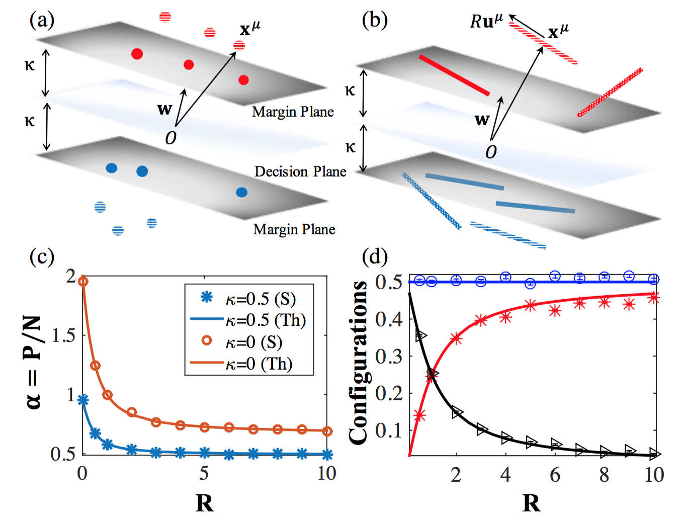
Figure 1: (a) Linear classification of points. (solid) points on the margin, (striped) internal points. (b) Linear classification of line segments. (solid) lines embedded in the margin, (dotted) lines touching the margin, (striped) interior lines. (c) Capacity $\alpha=P/N$ of a network $N=200$ as a function of $R$ with margins $\kappa=0$ (red) and $\kappa=0.5$ (blue). Theoretical predictions (lines) and numerical simulation (markers, see SM for details) are shown. (d) Fraction of different line configurations at capacity with $\kappa=0$. (red) lines in the margin, (blue) lines touching the margin, (black) internal lines.

Replica theory:

The existence of a weight vector $\mathbf{w}$ that can successfully classify the line segments depends upon the statistics of the segments. We consider random line segments where the components of $\mathbf{x}^{\mu}$ and $\mathbf{u}^{\mu}$ are i.i.d. Gaussians with zero mean and unit variance, and random binary labels $y^{\mu}$. We study the thermodynamic limit where the dimensionality $N\rightarrow\infty$ and number of segments $P\rightarrow\infty$ with finite $\alpha=P/N$ and $R$. Following Gardner gardner1988space we compute the average of $\log V$ where $V$ is the volume of the space of perceptron solutions:

$$V=\int_{\left\|\mathbf{w}\right\|^{2}=N}d^{N}\mathbf{w}\>\prod_{\mu=1}^{P}\Theta\left(h_{0}^{\mu}-R\left|h^{\mu}\right|-\kappa\right).$$ (1)

$\Theta(x)$ is the Heaviside step function. According to replica theory, the fields are described as sums of random Gaussian fields $h_{0}^{\mu}=t_{0}^{\mu}+z_{0}^{\mu}$ and $h^{\mu}=t^{\mu}+z^{\mu}$ where $t_{0}$ and $t$ are quenched components arising from fluctuations in the input vectors $\mathbf{x}^{\mu}$ and $\mathbf{u}^{\mu}$ respectively, and the $z_{0}$, $z$ fields represent the variability in $h_{0}^{\mu}$ and $h^{\mu}$ resulting from different solutions of $\mathbf{w}$. These fields must obey the constraint $z_{0}+t_{0}-R\left|z+t\right|\geq\kappa.$ The capacity function $\alpha_{1}(\kappa,R)$ (the subscript $1$ denotes the dimensionality of the manifolds) describes for which $P/N$ ratio the perceptron solution volume shrinks to a unique weight vector. The reciprocal of the capacity is given by the replica symmetric calculation (details provided in supplementary materials, SM):

$$\alpha_{1}^{-1}(\kappa,R)=\left\langle\min_{z_{0}+t_{0}-R\left|z+t\right|\geq\kappa}\frac{1}{2}\left[z_{0}^{2}+z^{2}\right]\right\rangle_{t_{0},t}$$ (2)

where the average is over the Gaussian statistics of $t_{0}$ and $t$. To compute Eq. (2), three regimes need to be considered. First, when $t_{0}$ is large enough so that $t_{0}>\kappa+R\left|t\right|$, the minimum occurs at $z_{0}=z=0$ which does not contribute to the capacity. In this regime, $h_{0}^{\mu}>\kappa$ and $h^{\mu}>0$ implying that neither of the two segment endpoints reach the margin. In the other extreme, when $t_{0}<\kappa-R^{-1}|t|$, the minimum is given by $z_{0}=\kappa-t_{0}$ and $z=-\left|t\right|$, i.e. $h_{0}^{\mu}=\kappa$ and $h^{\mu}=0$ indicating that both endpoints of the line segment lie on the margin planes. In the intermediate regime where $\kappa-R^{-1}\left|t\right|<t_{0}<\kappa+R\left|t\right|$, $z_{0}=\kappa-t_{0}+R|z+t$—, i.e., $h_{0}^{\mu}-R|h^{\mu}|=\kappa$ but $h_{0}^{\mu}>\kappa$, corresponding to only one of the line segment endpoints touching the margin. In this regime, the solution is given by minimizing the function $(R\left|z+t\right|+\kappa-t_{0})^{2}+z^{2}$ with respect to $z$. Combining these contributions, we can write the perceptron capacity of line segments:

$$\alpha_{1}^{-1}(\kappa,R) = \int_{-\infty}^{\infty}Dt\int_{\kappa-R^{-1}|t|}^{\kappa+R|t|}Dt_{0}\frac{\left(R\left|t\right|+\kappa-t_{0}\right)^{2}}{R^{2}+1}$$ (3)

$$+ \int_{-\infty}^{\infty}Dt\int_{-\infty}^{\kappa-R^{-1}|t|}Dt_{0}\left[(\kappa-t_{0})^{2}+t^{2}\right]\quad\quad$$

with integrations over the Gaussian measure, $Dx\equiv\frac{1}{\sqrt{2\pi}}e^{-\frac{1}{2}x^{2}}dx$. It is instructive to consider special limits. When $R\rightarrow 0,$ Eq. (3) reduces to $\alpha_{1}(\kappa,0)=\alpha_{0}(\kappa)$ where $\alpha_{0}(\kappa)$ is Gardner’s original capacity result for perceptrons classifying $P$ points (the subscript $0$ stands for zero-dimensional manifolds) with margin $\kappa$ 1-(a). Interestingly, when $R=1$, then $\alpha_{1}(\kappa,1)=\frac{1}{2}\alpha_{0}(\kappa/\sqrt{2})$. This is because when $R=1$ there are no statistical correlations between the line segment endpoints and the problem becomes equivalent to classifying $2P$ random points with average norm $\sqrt{2N}$ .

Finally, when $R\rightarrow\infty$, the capacity is further reduced: $\alpha_{1}^{-1}(\kappa,\infty)=\alpha_{0}^{-1}(\kappa)+1$. This is because when $R$ is large, the segments become unbounded lines. In this case, the only solution is for $\mathbf{w}$ to be orthogonal to all $P$ line directions. The problem is then equivalent to classifying $P$ center points in the $N-P$ null space of the line directions, so that at capacity $P=\alpha_{0}(\kappa)(N-P)$.

We see this most simply at zero margin, $\kappa=0$. In this case, Eq. (3) reduces to a simple analytic expression for the capacity: $\alpha_{1}^{-1}(0,R)=\frac{1}{2}+\frac{2}{\pi}\arctan R$ (SM). The capacity is seen to decrease from $\alpha_{1}(0,R=0)=2$ to $\alpha_{1}(0,R=1)=1$ and $\alpha_{1}(0,R=\infty)=\frac{2}{3}$ for unbounded lines. We have also calculated analytically the distribution of the center and direction fields $h_{0}^{\mu}$ and $h^{\mu}$ abbott1989universality . The distribution consists of three contributions, corresponding to the regimes that determine the capacity. One component corresponds to line segments fully embedded in these planes. The fraction of these manifolds is simply the volume of phase space of $t$ and $t_{0}$ in the last term of Eq. (3). Another fraction, given by the volume of phase space in the first integral of (3) corresponds to line segments touching the margin planes at only one endpoint. The remainder of the manifolds are those interior to the margin planes. Fig. 1 shows that our theoretical calculations correspond nicely with our numerical simulations for the perceptron capacity of line segments, even with modest input dimensionality $N=200$. Note that as $R\rightarrow\infty$, half of the manifolds lie in the plane while half only touch it; however, the angles between these segments and the margin planes approach zero in this limit. As $R\rightarrow 0$ , half of the points lie in the plane abbott1989universality .

$D$-dimensional balls:

Higher dimensional manifolds arise from multiple sources of variability and their nonlinear effects on the neural responses. An example is varying stimulus orientation, resulting in two-dimensional object manifolds under the cosine tuning function (Fig. 2(a)). Linear classification of these manifolds depends only upon the properties of their convex hulls de2000computational . We consider simple convex hull geometries as $D$-dimensional balls embedded in $N$-dimensions: $\left\{\mathbf{x}^{\mu}+R\sum_{i=1}^{D}s_{i}\mathbf{u}_{i}^{\mu}\right\}$, so that the $\mu$-th manifold is centered at the vector $\mathbf{x}^{\mu}\in\mathcal{R}^{N}$ and its extent is described by a set of $D$ basis vectors $\left\{\mathbf{u}_{i}^{\mu}\in\mathcal{R}^{N},\>i=1,...,D\right\}$. The points in each manifold are parameterized by the $D$-dimensional vector $\vec{s}\in\mathcal{R}^{D}$ whose Euclidean norm is constrained by: $\left\|\vec{s}\right\|\leq 1$ and the radius of the balls are quantified by $R$ .

Statistically, all components of $\mathbf{x}^{\mu}$ and $\mathbf{u}_{i}^{\mu}$ are i.i.d. Gaussian random variables with zero mean and unit variance. We define $h_{0}^{\mu}=N^{-1/2}y^{\mu}\mathbf{w}\cdot\mathbf{x}^{\mu}$ as the field induced by the manifold centers and $h_{i}^{\mu}=N^{-1/2}y^{\mu}\mathbf{w}\cdot\mathbf{u}_{i}^{\mu}$ as the $D$ fields induced by each of the basis vectors and with normalization $\left\|\mathbf{w}\right\|=\sqrt{N}$. To classify all the points on the manifolds correctly with margin $\kappa$, $\mathbf{w}\in\mathcal{R}^{N}$ must satisfy the inequality $h_{0}^{\mu}-R||\vec{h}^{\mu}||\geq\kappa$ where $||\vec{h}^{\mu}||$ is the Euclidean norm of the $D$-dimensional vector $\vec{h}^{\mu}$ whose components are $h_{i}^{\mu}$ . This corresponds to the requirement that the field induced by the points on the $\mu$-th manifold with the smallest projection on $\mathbf{w}$ be larger than the margin $\kappa$.

We solve the replica theory in the limit of $N,\,P\rightarrow\infty$ with finite $\alpha=P/N$, $D$, and $R$. The fields for each of the manifolds can be written as sums of Gaussian quenched and entropic components, $\left(t_{0}\in\mathcal{R},\>\vec{t}\in\mathcal{R}^{D}\right)$ and $\left(z_{0}\in\mathcal{R},\>\vec{z}\in\mathcal{R}^{D}\right)$ , respectively. The capacity for $D$-dimensional manifolds is given by the replica symmetric calculation (SM):

$$\alpha_{D}^{-1}(\kappa,R)=\left\langle\min_{t_{0}+z_{0}-R\left\|\vec{t}+\vec{z}\right\|>\kappa}\frac{1}{2}\left[z_{0}^{2}+\left\|\vec{z}\right\|^{2}\right]\right\rangle_{t_{0},\vec{t}}.$$ (4)

The capacity calculation can be partitioned into three regimes. For large $t_{0}>\kappa+Rt$, where $t=\left\|\vec{t}\right\|$, $z_{0}=0$ and $\vec{z}=0$ corresponding to manifolds which lie interior to the margin planes of the perceptron. On the other hand, when $t_{0}<\kappa-R^{-1}t$, the minimum is obtained at $z_{0}=\kappa-t_{0}$ and $\vec{z}=-\vec{t}$ corresponding to manifolds which are fully embedded in the margin planes. Finally, in the intermediate regime, when $\kappa-R^{-1}t<t_{0}<\kappa+Rt$, $z_{0}=R\left\|\vec{t}+\vec{z}\right\|-t_{0}+\kappa$ but $\vec{z}\neq-\vec{t}$ indicating that these manifolds only touch the margin plane. Decomposing the capacity over these regimes and integrating out the angular components, the capacity of the perceptron can be written as:

$$\alpha_{D}^{-1}(\kappa,R) = \int_{0}^{\infty}dt\,\chi_{D}(t)\int_{\kappa-\frac{1}{R}t}^{\kappa+Rt}Dt_{0}\frac{\left(Rt+\kappa-t_{0}\right)^{2}}{R^{2}+1}$$ (5)

$$+ \int_{0}^{\infty}dt\,\chi_{D}(t)\int_{-\infty}^{\kappa-\frac{1}{R}t}Dt_{0}\left[\left(\kappa-t_{0}\right)^{2}+t^{2}\right]\qquad$$

where $\chi_{D}(t)=\frac{2^{1-\frac{D}{2}}}{\Gamma(\frac{D}{2})}t^{D-1}e^{-\frac{1}{2}t^{2}}$ is the D-Dimensional Chi probability density function. For large $R\rightarrow\infty$, Eq. (5) reduces to: $\alpha_{D}^{-1}(\kappa,\infty)=\alpha_{0}^{-1}(\kappa)+D$ which indicates that $\mathbf{w}$ must be in the null space of the $PD$ basis vectors $\left\{\mathbf{u}_{i}^{\mu}\right\}$ in this limit. This case is equivalent to the classification of $P$ points (the projections of the manifold centers) by a perceptron in the $N-PD$ dimensional null space.

To probe the fields, we consider the joint distribution of the field induced by the center, $h_{0}$, and the norm of the fields induced by the manifold directions, $h\equiv\left\|\vec{h}\right\|$ . There are three contributions. The first term corresponds to $h_{0}-Rh>\kappa$, i.e. balls that lie interior to the perceptron margin planes; the second component corresponds to $h_{0}-Rh=\kappa$ but $h>0$, i.e. balls that touch the margin planes; and the third contribution represents the fraction of balls obeying $h_{0}=\kappa$ and $h=0$, i.e. balls fully embedded in the margin. The dependence of these contributions on $R$ for $D=2$ is shown in Fig. 2(b). Interestingly, when $\kappa=0$ , the case of $R=1$ is particularly simple for all $D$ . The capacity is $\alpha_{D}=2/(D+1)$ ; in addition, the fraction of embedded and interior balls are equal and the fraction of touching balls have a maximum, see Fig. 2(b) and SM.

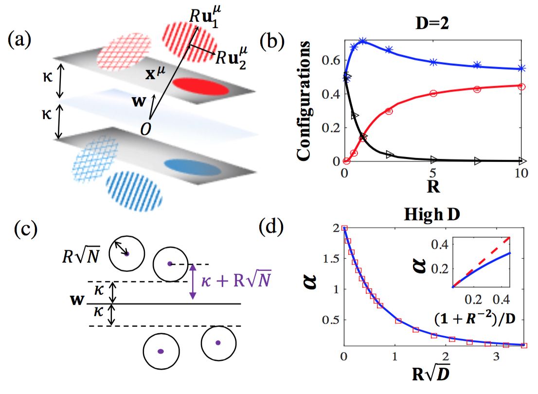
Figure 2: Random $D$-dimensional balls: (a) Linear classification of $D=2$ balls. (b) Fraction of 2-$D$ ball configurations as a function of $R$ at capacity with $\kappa=0$, comparing theory (lines) with simulations (markers). (red) balls embedded in the plane, (blue) balls touching the plane, (black) interior balls. (c) Linear classification of balls with $D=N$ at margin $\kappa$ (black circles) is equivalent to point classification of centers with effective margin $\kappa+R\sqrt{N}$ (purple points). (d) Capacity $\alpha=P/N$ for $\kappa=0$ for large $D=50$ and $R\propto D^{-1/2}$ as a function of $R\sqrt{D}$. (blue solid) $\alpha_{D}(0,R)$ compared with $\alpha_{0}(R\sqrt{D})$ (red square). (Inset) Capacity $\alpha$ at $\kappa=0$ for $0.35\leq R\leq 20$ and $D=20$: (blue) theoretical $\alpha$ compared with approximate form $(1+R^{-2})/D$ (red dashed).

In a number of realistic problems, the dimensionality $D$ of the object manifolds could be quite large. Hence, we analyze the limit $D\gg 1$. In this situation, for the capacity to remain finite, $R$ has to be small, scaling as $R\propto D^{-\frac{1}{2}}$, and the capacity is $\alpha_{D}(\kappa,R)\approx\alpha_{0}(\kappa+R\sqrt{D})$. In other words, the problem of separating $P$ high dimensional balls with margin $\kappa$ is equivalent to separating $P$ points but with a margin $\kappa+R\sqrt{D}$. This is because when the distance of the closest point on the $D$-dimensional ball to the margin plane is $\kappa$, the distance of the center is $\kappa+R\sqrt{D}$ (see Fig. 2). When $R$ is larger, the capacity vanishes as $\alpha_{D}(0,R)\approx\left(1+R^{-2}\right)/D$. When $D$ is large, making $\mathbf{w}$ orthogonal to a significant fraction of high dimensional manifolds incurs a prohibitive loss in the effective dimensionality. Hence, in this limit, the fraction of manifolds that lie in the margin plane is zero. Interestingly, when $R$ is sufficiently large, $R\propto\sqrt{D}$, it becomes advantageous for $\mathbf{w}$ to be orthogonal to a finite fraction of the manifolds.

$L_{p}$ balls:

To study the effect of changing the geometrical shape of the manifolds, we replace the Euclidean norm constraint on the manifold boundary by a constraint on their $L_{p}$ norm. Specfically, we consider $D$-dimensional manifolds $\left\{x^{\mu}+R\sum_{i=1}^{D}s_{i}u_{i}^{\mu}\right\}$ where the $D$ dimensional vector $\vec{s}$ parameterizing points on the manifolds is constrained: $\left\|\vec{s}\right\|_{p}\leq 1$. For $1<p<\infty$, these $L_{p}$ manifolds are smooth and convex. Their linear classification by a vector $\mathbf{w}$ is determined by the field constraints $h_{0}^{\mu}-R||\vec{h}{}^{\mu}||_{q}\geq\kappa$ where, as before, $h_{0}^{\mu}$ are the fields induced by the centers, and $||\vec{h}^{\mu}||_{q}$, $q=p/(p-1)$, are the $L_{q}$ dual norms of the $D$-dimensional fields induced by $\mathbf{u}_{i}^{\mu}$ (SM). The resultant solutions are qualitatively similar to what we observed with $L_{2}$ ball manifolds.

However, when $p\leq 1$, the convex hull of the manifold becomes faceted, consisting of vertices, flat edges and faces. For these geometries, the constraints on the fields associated with a solution vector $\mathbf{w}$ becomes: $h_{0}^{\mu}-R\max_{i}\left|h_{i}^{\mu}\right|\geq\kappa$ for all $p<1$ . We have solved in detail the case of $D=2$ (SM). There are four manifold classes: interior; touching the margin plane at a single vertex point; a flat side embedded in the margin; and fully embedded. The fractions of these classes are shown in Fig. 3.

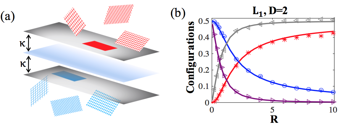
Figure 3: $L_{1}$ balls: (a) Linear classification of 2-$D$ $L_{1}$ balls. (b) Fraction of manifold configurations as a function of radius $R$ at capacity with $\kappa=0$ comparing theory (lines) to simulations (markers). (red) entire manifold embedded, (blue) manifold touching margin at a single vertex, (gray) manifold touching with two corners (one side), (purple) interior manifold.

Discussion:

We have extended Gardner’s theory of the linear classification of isolated points to the classification of continuous manifolds. Our analysis shows how linear separability of the manifolds depends intimately upon the dimensionality, size and shape of the convex hulls of the manifolds. Some or all of these properties are expected to differ at different stages in the sensory hierarchy. Thus, our theory enables systematic analysis of the degree to which this reformatting enhances the capacity for object classification at the higher stages of the hierarchy.

We focused here on the classification of fully observed manifolds and have not addressed the problem of generalization from finite input sampling of the manifolds. Nevertheless, our results about the properties of maximum margin solutions can be readily utilized to estimate generalization from finite samples. The current theory can be extended in several important ways. Additional geometric features can be incorporated, such as non-uniform radii for the manifolds as well as heteogeneous mixtures of manifolds. The influence of correlations in the structure of the manifolds as well as the effect of sparse labels can also be considered. The present work lays the groundwork for a computational theory of neuronal processing of objects, providing quantitative measures for assessing the properties of representations in biological and artificial neural networks.

- (1) J. J. DiCarlo and D. D. Cox, Trends in Cognitive Sciences 11, 333 (2007).
- (2) M. Pagan, L. S. Urban, M. P. Wohl, and N. C. Rust, Nature Neuroscience 16, 1132 (2013).
- (3) A. Alemi-Neissi, F. B. Rosselli, and D. Zoccolan, The Journal of Neuroscience 33, 5939 (2013).
- (4) J. K. Bizley and Y. E. Cohen, Nature Reviews Neuroscience 14, 693 (2013).
- (5) E. M. Meyers, M. Borzello, W. A. Freiwald, and D. Tsao, The Journal of Neuroscience 35, 7069 (2015).
- (6) R. F. Schwarzlose, J. D. Swisher, S. Dang, and N. Kanwisher, Proceedings of the National Academy of Sciences 105, 4447 (2008).
- (7) J. A. Gottfried, Nature Reviews Neuroscience 11, 628 (2010).
- (8) C. P. Hung, G. Kreiman, T. Poggio, and J. J. DiCarlo, Science 310, 863 (2005).
- (9) W. A. Freiwald and D. Y. Tsao, Science 330, 845 (2010).
- (10) C. F. Cadieu, H. Hong, D. L. Yamins, N. Pinto, D. Ardila, E. A. Solomon, N. J. Majaj, and J. J. Di- Carlo, PLoS Comput Biol 10, e1003963 (2014).
- (11) E. Kobatake and K. Tanaka, Journal of neurophysiology 71, 856 (1994).
- (12) N. C. Rust and J. J. DiCarlo, The Journal of Neuroscience 30, 12978 (2010).
- (13) M. L. Minsky and S. A. Papert, Perceptrons - Expanded Edition: An Introduction to Computational Geometry (MIT press Boston, MA:, 1987).
- (14) E. Gardner, Europhysics Letters 4, 481 (1987).
- (15) T. Serre, L. Wolf, and T. Poggio, in IEEE Conference on Computer Vision and Pattern Recognition, CVPR (IEEE, 2005), vol. 2, pp. 994–1000.
- (16) I. Goodfellow, H. Lee, Q. V. Le, A. Saxe, and A. Y. Ng, in Advances in Neural Information Processing Systems (2009), pp. 646–654.
- (17) M. A. Ranzato, F. J. Huang, Y.-L. Boureau, and Y. Le- Cun, in IEEE Conference on Computer Vision and Pattern Recognition, CVPR (IEEE, 2007), pp. 1–8.
- (18) Y. Bengio, Foundations and Trends in Machine Learning 2, 1 (2009).
- (19) E. Gardner, Journal of physics A: Mathematical and General 21, 257 (1988).
- (20) A. Engel, C. Van den Broeck, and C. Broeck, Statistical Mechanics of Learning (Cambridge University Press, 2001).
- (21) M. Advani, S. Lahiri, and S. Ganguli, Journal of Statistical Mechanics: Theory and Experiment 2013, P03014 (2013).
- (22) N. Brunel, V. Hakim, P. Isope, J.-P. Nadal, and B. Bar- bour, Neuron 43, 745 (2004).
- (23) R. Rubin, R. Monasson, and H. Sompolinsky, Physical Review Letters 105, 218102 (2010).
- (24) H. Sompolinsky, N. Tishby, and H. S. Seung, Physical Review Letters 65, 1683 (1990).
- (25) M. Opper and D. Haussler, Physical Review Letters 66, 2677 (1991).
- (26) D. J. Amit, K. Wong, and C. Campbell, Journal of Physics A: Mathematical and General 22, 2039 (1989).
- (27) R. Monasson, Journal of Physics A: Mathematical and General 25, 3701 (1992).
- (28) V. Vapnik, Statistical Learning Theory, vol. 1 (Wiley New York, 1998).
- (29) L. F. Abbott and T. B. Kepler, Journal of Physics A: Mathematical and General 22, 2031 (1989).
- (30) M. De Berg, M. Van Kreveld, M. Overmars, and O. C. Schwarzkopf, Computational geometry (Springer, 2000).