On overdamping phenomena in gyroscopic systems composed of high-loss and lossless components

Abstract

Using a Lagrangian framework, we study overdamping phenomena in gyroscopic systems composed of two components, one of which is highly lossy and the other is lossless. The losses are accounted by a Rayleigh dissipative function. As we have shown previously, for such a composite system the modes split into two distinct classes, high-loss and low-loss, according to their dissipative behavior. A principal result of this paper is that for any such system a rather universal phenomenon of selective overdamping occurs. Namely, first of all the high-loss modes are all overdamped, i.e., non-oscillatory, as are an equal number of low-loss modes. Second of all, the rest of the low-loss modes remain oscillatory (i.e., the underdamped modes) each with an extremely high quality factor (Q-factor) that actually increases as the loss of the lossy component increases. We prove that selective overdamping is a generic phenomenon in Lagrangian systems with gyroscopic forces and give an analysis of the overdamping phenomena in such systems. Moreover, using perturbation theory, we derive explicit formulas for upper bound estimates on the amount of loss required in the lossy component of the composite system for the selective overdamping to occur in the generic case, and give Q-factor estimates for the underdamped modes. Central to the analysis is the introduction of the notion of a “dual” Lagrangian system and this yields significant improvements on some results on modal dichotomy and overdamping. The effectiveness of the theory developed here is demonstrated by applying it to an electric circuit with a gyrator element and a high-loss resistor.

1 Introduction

In this paper we use the Lagrangian framework introduced in [FigWel2] to study the dissipative properties and overdamping phenomena of two-component composite systems composed of a high-loss and lossless components, when the system also possesses gyroscopic properties. This study applies to any finite-dimensional linear Lagrangian system, with gyroscopic and dissipative forces, provided (i) it has a nonnegative Hamiltonian, and (ii) losses are accounted by a Rayleigh dissipative function, [Pars, Sec. 10.11, 10.12], [Gant, Sec. 8, 9, 46]. Such physical systems include, in particular, many different types of rotating damped mechanical systems such as fly wheels [Kelv88I, §345], MEMS vibratory gyroscopes [AcSh08], [ApoTay05], electric networks with gyrators [Tell48], [CarGio64], or, in electrodynamics, a moving point charge driven by the Lorentz force due to a static electromagnetic field [Gold].

The rest of the paper is organized as follows. In the remainder of this introduction, we will first introduce in Subsection 1.1 a model for a two-component composite system with a high-loss and a lossless component based on our Lagrangian framework introduced in [FigWel2], which is overviewed in Subsections 1.1 and 1.5. We introduce then in Subsection 1.2 the definition of overdamped and underdamped modes which is followed by a brief discussion on examples illustrating some of the subtleties of overdamping phenomena in gyroscopic-dissipative systems. We motivate our approach to overdamping in Subsection 1.3 by indicating its relevance in the development of a theory of broadband absorption suppression in magnetic composites. We give then an overview of the selective overdamping phenomenon, which was first introduced in [FigWel2], and discuss its potential as a mechanism for significant broadband absorption suppression in composites. Finally, in Subsection 1.4 we give a brief summary of the main results of this paper on modal dichotomy and overdamping phenomena in gyroscopic-dissipative systems.

In Section 2, we illustrate our main results based on a simple example of an electric circuit with a resistor (lossy element) and a gyrator (gyroscopic element). Using this example we examine analytically and numerically the modal dichotomy and overdamping phenomena. Next, in Section 3, we introduce the notion of the “dual” of a Lagrangian system which plays a key role in the study of the modal dichotomy and overdamping. Then we discuss the spectral problems that arise in studying the dissipative properties of eigenmodes of Lagrangian systems. Finally, Section 4 is devoted to the precise formulation of all significant results in this paper in the form of theorems, propositions, etc. and their proofs.

1.1 Overview of our model

The general Euler-Lagrange equations of motion of the gyroscopic-dissipative (Lagrangian) systems considered in this paper are of the form

$$\alpha\ddot{Q}+\left(2\theta+\beta R\right)\dot{Q}+\eta Q=0\qquad\text{(evolution equations),}$$ (1)

$$0\leq\beta\qquad\text{(loss parameter),}$$ (2)

where $\dot{Q}=\partial_{t}Q$, $\ddot{Q}=\partial_{t}^{2}Q$, $\beta$ is a scalar perturbation parameter ($\beta$ is a dimensionless loss parameter which we introduce to scale the intensity of dissipation), and the $N\times N$ matrices $\alpha$, $\eta$, $\theta$, $R$ have the properties that their matrix entries are real and

$$\alpha^{\mathrm{T}}=\alpha>0,\text{ }\eta^{\mathrm{T}}=\eta\geq 0,\text{ }\theta^{\mathrm{T}}=-\theta,\text{ \ }R^{\mathrm{T}}=R\geq 0,$$ (3)

($\mathrm{T}$ denotes the transpose of a matrix). We also assume the rank $N_{R}$ of the matrix $R$ is positive:

$$0<N_{R}=\operatorname{rank}R$$ (4)

(i.e., the dimension $N_{R}$ of the range of $R$ is positive). We will refer to this dissipative system with equations of motion (1) as gyroscopic if $\theta\not=0$ and non-gyroscopic if $\theta=0$.

Here the terms involving $\beta R$ and $\theta$ correspond respectively to dissipative and gyroscopic forces of the Lagrangian system, in which the Lagrangian $\mathcal{L}$ and the Rayleigh dissipation function $\mathcal{R}$ are the following quadratic forms

$$\mathcal{L}=\mathcal{L}\left(Q,\dot{Q}\right)=\frac{1}{2}\left[\begin{array}[c]{l}\dot{Q}\\ Q\end{array}\right]^{\mathrm{T}}\left[\begin{array}[c]{ll}\alpha&\theta\\ \theta^{\mathrm{T}}&-\eta\end{array}\right]\left[\begin{array}[c]{l}\dot{Q}\\ Q\end{array}\right]\qquad\text{(the Lagrangian),}$$ (11)

$$\mathcal{R}=\mathcal{R}\left(\dot{Q}\right)=\frac{1}{2}\dot{Q}^{\mathrm{T}}\beta R\dot{Q}\qquad\text{(the Rayleigh dissipation function).}$$ (12)

Eqs. (1) are the Euler-Lagrange (EL) equations with the dissipative forces $\frac{\partial\mathcal{R}}{\partial\dot{Q}}$, namely,

$$\frac{d}{dt}\left(\frac{\partial\mathcal{L}}{\partial\dot{Q}}\right)-\frac{\partial\mathcal{L}}{\partial Q}=-\frac{\partial\mathcal{R}}{\partial\dot{Q}}\qquad\text{(EL equations with dissipative forces),}$$ (13)

where the generalized coordinates $Q$ and velocities $\dot{Q}$ take values in the Euclidean space $\mathbb{R}^{N}$. The Hamiltonian $\mathcal{H}\geq 0$ corresponding to the Lagrangian $\mathcal{L}$ can be represented as a function $Q$ and $\dot{Q}$ in the following form:

$$\mathcal{L}=\mathcal{T}-\mathcal{V},\qquad 0\leq\mathcal{H}=\mathcal{T}+\mathcal{V=}\frac{1}{2}\dot{Q}^{\mathrm{T}}\alpha\dot{Q}+\frac{1}{2}Q^{\mathrm{T}}\eta Q\qquad\text{ (Hamiltonian),}$$ (14)

where $\mathcal{T}$ and $\mathcal{V}$ are respectively the kinetic and the potential energies of the form

$$\mathcal{T} =\mathcal{T}(\dot{Q},Q)=\frac{1}{2}\dot{Q}^{\mathrm{T}}\alpha\dot{Q}+\frac{1}{2}\dot{Q}^{\mathrm{T}}\theta Q,$$ (15)

$$\mathcal{V} =\mathcal{V}(\dot{Q},Q)=\frac{1}{2}Q^{\mathrm{T}}\eta Q-\frac{1}{2}\dot{Q}^{\mathrm{T}}\theta Q.$$

The solutions of Eq. (1) satisfy the energy balance equation:

$$-\partial_{t}\mathcal{H}=2\mathcal{R}\geq 0\qquad\text{(energy balance equation),}$$ (16)

which expresses the energy lost per unit time, where the system energy (or stored energy) is represented by the Hamiltonian $\mathcal{H}\geq 0$, the dissipated power is $2\mathcal{R}\geq 0$.

The model of a two-component composite system (TCCS) made of a lossy and a lossless components incorporates losses represented by the Rayleigh dissipation matrix $R$ and the loss fraction parameter

$$\delta_{R}=\frac{N_{R}}{N}\qquad\text{(loss fraction).}$$ (17)

The lossy component of system can be roughly characterized by the range $\operatorname{Ran}R$ of the matrix $R$ with the lossless component being its nullspace $\operatorname{Ker}R$. The loss fraction $\delta_{R}$ defined by (17) is then interpreted as the ratio of the degrees of freedom susceptible to losses (i.e., $N_{R}=\dim\operatorname{Ran}R$) to the degrees of freedom of the entire system (i.e., $N$). When considering a TCCS model we assume that the following condition is satisfied

$$0<\delta_{R}<1\qquad\text{(loss fraction condition),}$$ (18)

that is, the nonzero matrix $R$ does not have full rank (i.e., $R$ is rank deficient).

A function $Q=Q\left(t\right)=Q\left(t,\beta\right)$ is a solution of Eq. (1) if $Q$, $\dot{Q}=\partial_{t}Q$, and $\ddot{Q}=\partial_{t}^{2}Q$ are continuous functions of the independent variable $t$ into $\mathbb{C}^{N}$ and satisfy (1) for all $t\in\mathbb{R}$. The eigenmodes of the Lagrangian system are solutions of Eq. (1) of the form

$$Q\left(t\right)=qe^{-\mathrm{i}\zeta t},\text{ }0\not=q\in\mathbb{C}^{N}\qquad\text{(eigenmode).}$$ (19)

Its frequency $\omega$ and damping factor $\gamma$ are defined in terms of the real and imaginary part of $\zeta$, i.e.,

$$\omega=\operatorname{Re}\zeta\quad\text{(frequency),}\qquad 0\leq\gamma=-\operatorname{Im}\zeta\quad\text{(damping factor).}$$ (20)

The damping factor is nonnegative due to the fact that for such a mode the energy balance equation (16) still holds, but now in the complex inner product $\left(a,b\right)=a^{\ast}b$ for $a$,$b\in\mathbb{C}^{N}$, where $\ast$ denotes the complex conjugate transpose of vectors or matrices.

An important figure-of-merit, which characterizes the performance of the dissipative system (1), is the quality factor (Q-factor) that can be naturally introduced in a few not entirely equivalent ways (see, for instance, [Pain, pp. 47, 70, and 71]). When the system is in the time-harmonic state (19), with frequency and damping factor (20), the quality factor $Q_{\zeta}$ is most commonly defined as the reciprocal of the relative rate of energy dissipation per temporal cycle, that is,

$$Q_{\zeta}=2\pi\frac{\text{energy stored}}{\text{energy lost per cycle}}=\left|\omega\right|\frac{\mathcal{H}}{-\partial_{t}\mathcal{H}}=\frac{1}{2}\frac{\left|\omega\right|}{\gamma}\text{\quad(Q-factor),}$$ (21)

with the convention $Q_{\zeta}=+\infty$ if $\gamma=0$ and $\omega\not=0$ and $Q_{\zeta}=0$ if $\zeta=0$.

1.2 The subtleties of overdamping phenomena

For the purposes of this paper, the following definitions of an overdamped and an underdamped mode will be sufficient.

Definition 1 (overdamped mode)

Any eigenmode (19) of the Lagrangian system (1) with time-dependency $e^{-\mathrm{i}\zeta\left(\beta\right)t}$ for which there exists a $\beta^{\prime}\geq 0$ such that its frequency $\omega$ has the property

$$\omega=\operatorname{Re}\zeta\left(\beta\right)=0,\quad\text{for all }\beta>\beta^{\prime}\qquad\text{(overdamped),}$$ (22)

or

$$\omega=\operatorname{Re}\zeta\left(\beta\right)\not=0,\quad\text{for all }\beta>\beta^{\prime}\qquad\text{\ (underdamped),}$$ (23)

will be called an overdamped mode (and is said to be overdamped) or underdamped mode (and is said to be underdamped), respectively.

In order to appreciate the subtleties of overdamping that we want to study in this paper, we will give some simple examples and recall some previous results on overdamping.

Example 2 (spring-mass-damper)

For the simplest mechanical (non-gyroscopic) system of a spring-mass-damper system with one degree-of-freedom ($N=1$), the equations of motion of this Lagrangian system (1) in standard form is

$$m\ddot{x}+\beta R\dot{x}+kx=0,$$

where $\alpha=m>0$ is the mass, $\beta R$ is the damping (with $R>0$, $\beta\geq 0$, $\delta_{R}=N_{R}/N=1$), and $\eta=k>0$ is the spring constant, $Q=x$ is the displacement from equilibrium at $x=0$, $\dot{Q}=\dot{x}$ is its velocity, and $\theta=0$. This mechanical system has the Lagrangian, Hamiltonian, and Rayleigh dissipation function:

$$\mathcal{L}=\mathcal{T}-\mathcal{V},\text{ }\mathcal{H}=\mathcal{T}+\mathcal{V},\text{ }\mathcal{R}=\frac{1}{2}\beta R\left|\dot{x}\right|^{2},\text{ }\mathcal{T}=\frac{1}{2}m\left|\dot{x}\right|^{2},\text{ }\mathcal{V}=\frac{1}{2}k\left|x\right|^{2},$$

where $\mathcal{T}$, $\mathcal{V}$ are the kinetic and potential energy, respectively. The eigenmodes of the system have time-dependency $e^{-\mathrm{i}\zeta_{j}\left(\beta\right)t}$, $j=1,2$ with

$$\zeta_{j}\left(\beta\right)=-\mathrm{i}\frac{\beta R}{2m}+\left(-1\right)^{j}\sqrt{\frac{k}{m}-\left(\frac{\beta R}{2m}\right)^{2}},\quad j=1,2.$$

Thus, all the modes of this system will be overdamped (according to our definition 1) once

$$\beta>\beta^{\prime}\text{, where }\beta^{\prime}=\frac{2\sqrt{mk}}{R}.$$

The simple example above illustrates a general result on overdamping for non-gyroscopic systems with only lossy components. The next theorem from [FigWel2, Theorem 17] (see also [Duff55], [BarLan92]) gives a precise statement of the result.

Theorem 3 (complete overdamping)

Suppose $\theta=0$ (i.e., a non-gyroscopic system) and $\delta_{R}=1$ (i.e., $R$ has full rank). Then there exists a $\beta^{\prime}>0$ such that if $\beta>\beta^{\prime}$ then all the eigenmodes of the Lagrangian system with equations of motion (1) are overdamped. In particular, we can take

$$\beta^{\prime}=2\frac{\omega_{\max}}{b_{\min}},$$

where

$$\omega_{\max}=\sqrt{\max\sigma\left(\alpha^{-1}\eta\right)},\text{ }b_{\min}=\min\sigma\left(\alpha^{-1}R\right)$$

and $\sigma\left(M\right)$ denotes spectrum of a square matrix $M$, i.e., the set of its eigenvalues.

Remark 4

Although it may not be immediately obvious, the spectrums $\sigma\left(\alpha^{-1}\eta\right)$ and $\sigma\left(\alpha^{-1}R\right)$ are subsets of $[0,\infty)$ since $\alpha^{-1}\eta$ and $\alpha^{-1}R$ are similar to positive semidefinite matrices:

$$\alpha^{-1}\eta=\sqrt{\alpha}^{-1}\left(\sqrt{\alpha}^{-1}\eta\sqrt{\alpha}^{-1}\right)\sqrt{\alpha},\text{ }\alpha^{-1}R=\sqrt{\alpha}^{-1}\left(\sqrt{\alpha}^{-1}R\sqrt{\alpha}^{-1}\right)\sqrt{\alpha},$$

$$\sqrt{\alpha}^{-1}\eta\sqrt{\alpha}^{-1}\geq 0,\sqrt{\alpha}^{-1}R\sqrt{\alpha}^{-1}\geq 0.$$

In particular, this implies $\beta^{\prime}\geq 0$ in the previous theorem.

The next example, which we will discuss in more detail later in this paper (see Example 45), shows that, unlike for non-gyroscopic systems, in gyroscopic systems it is entirely possible that all the modes can be underdamped when the loss fraction condition (18) fails to be satisfied.

Example 5 (no overdamping)

If $\alpha=\eta=R=\mathbf{1}$ (where $\mathbf{1}$ denotes the $N\times N$ identity matrix and hence $\delta_{R}=1$) and $0\not\in\sigma\left(\theta\right)$ then all the eigenmodes of the Lagrangian system with equations of motion (1) are underdamped for $\beta>0$.

Notice that in the mentioned examples and results the loss fraction condition (18) is not satisfied, namely $\delta_{R}=1$, and hence the dissipative (Lagrangian) system consists only of lossy components. But the question we are most interested in is: what overdamping phenomena can occur for a two-component composite system with a lossy and a lossless component when the loss fraction condition (18), that is, $0<\delta_{R}<1$, is satisfied? The answer is that (generically) some of the modes of the system will be overdamped and some will be underdamped, and we refer to this phenomenon as selective overdamping. In the next subsection, we will give a brief description of this phenomenon along with our motivation for its study, and in the subsection afterwards give an overview of our main results.

1.3 Motivation

An important motivation for our studies of two component dissipative gyroscopic system is the development of a theory of broadband absorption suppression in magnetic composites. Such a theory, we believe, can provide guiding principles for the design of broadband low-loss magnetic composites with functionality comparable to bulk magnetic materials. The development of theory requires a deeper understanding of the interplay between losses and magnetism manifested as gyroscopic effects. There are numerious applications of low loss magnetic materials. For instance, they are crucial components in many microwave, infrared, and optical devices [FMW55], [Hogan52], [ILB13], [Pozer12], [ZveKot97]. Detrimental to the performance of many such devices are the high losses associated with the magnetic materials in frequency ranges of interest, [Hogan52], [ZveKot97], and this is a major problem with many natural and synthetic magnetic materials.

The discussion above raises a question if such broadband absorption suppression in composites even possible? Quite remarkably, the answer is yes. This result was firmly established in [FigVit8], [FigVit10], [SmCh11], [SmCa13]. For instance, in [FigVit8] an example was given of a two-component dielectric medium composed of a high-loss and lossless components, namely, a magnetophotonic crystal (MPCs) consisting of a finite stack of alternating lossy magnetic and lossless dielectric layers. They showed that the magnetic composite could reduce the absorption (losses) by two orders of magnitude in the chosen frequency range compared to those of the uniform bulk magnetic material while simultaneously enhancing one of its desired magnetic properties, namely, nonreciprocal Faraday rotation. That example demonstrated that it is possible to design a composite material/system which can have a desired property comparable with a naturally occurring bulk substance but with significantly reduced losses.

In addition to this, an interesting and rather counterintuitive idea arose, which was first introduced in [FigVit8], and also recently noticed independently in [IOKS11] for MPCs. It is the idea that reduction of losses in the magnetic composite and enhancement of the magnetic properties/functionality might actually be more substantial when the lossy magnetic component is replaced by another with even higher losses.

What is the origin of that seemingly counterintuitive behavior in composites? In order to understand the general mechanism for this behavior, we developed in [FigWel1] a model, based on the linear response theory from [FigSch1] and [FigSch2], for two-component composite systems with a high-loss and lossless component and introduced in [FigWel2] a Lagrangian framework, based on the Lagrangian-Hamiltonian formulation of classical mechanics, in order to account for the physical properties of the composite system. We showed that for such composite systems the losses of the entire system become small provided that the lossy component is sufficiently lossy. This behavior can be explained by two important phenomena, namely, the modal dichotomy and overdamping.

As the focus of this paper is on the study of these two phenomena in gyroscopic-dissipative systems, we will provide a brief explaination from our studies in [FigWel1], [FigWel2] on how these phenomena contribute to the loss suppression. We introduce first a dimensionless loss parameter $\beta\geq 0$ which scales the dissipation in the lossy component of the system. We consider then the system eigenmodes, i.e., the states of the system in the absence of external forces with exponential time dependency of the form $e^{-\mathrm{i}\zeta t}=e^{-\frac{t}{T}}e^{-\mathrm{i}\operatorname{Re}\zeta t}$, where $\operatorname{Re}\zeta=\omega$ is the frequency, $-\operatorname{Im}\zeta=\gamma\geq 0$ is the damping factor, and $T_{\zeta}=\frac{1}{-\operatorname{Im}\zeta}$ is the relaxation time. To any such mode is associated its quality factor (Q-factor) $Q_{\zeta}=-\frac{1}{2}\frac{\left|\omega\right|}{\gamma}$, which is an important figure of merit that helps to characterize the performance of the dissipative composite system. Now as the losses in the lossy component of the composite system become sufficiently large, i.e., $\beta\gg 1$, the entire set of eigenmodes of the composite system splits into two classes, high-loss and low-loss modes, based on their dissipative properties. We refer to this phenomenon as the modal dichotomy. One important feature of this dichotomy is that the high-loss modes decay exponentially in time with both an extremely small relaxation time $T_{\zeta}$ and Q-factor $Q_{\zeta}$ that decrease with $T_{\zeta}\rightarrow 0$ and $Q_{\zeta}\rightarrow 0$ as $\beta\rightarrow\infty$. On the other hand, the low-loss modes have an extremely large relaxation time $T_{\zeta}$ which increases with $T_{\zeta}\rightarrow\infty$ as $\beta\rightarrow\infty$, whereas the Q-factor $Q_{\zeta}$ either decreases or increases with $Q_{\zeta}\rightarrow 0$ or $Q_{\zeta}\rightarrow\infty$, respectively, as $\beta\rightarrow\infty$ (as to this behavior of the Q-factor and whether such low-loss high-Q modes even exist, we address this in the next paragraph). Moreover, in Lagrangian systems, when the loss of the high-loss component exceeds a finite critical value, i.e., $\beta>\beta_{0}$, the frequencies of the all the high-loss eigenmodes become exactly zero, i.e., $\operatorname{Re}\zeta=0$ for $\beta>\beta_{0}$, a phenomenon known as overdamping. Consequently, when the composite is excited by external forces at frequencies ranges well separated from zero, the high-loss modes hardly respond to these excitations because they are overdamped with extremely small relaxation time, and hence do not contribute much to the entire composite losses.

This analysis leads to the important question: do such high-Q modes even exist in systems with a high-loss component? As discussed in [FigWel1], [FigWel2] the answer is yes, but not always and composites with a high-loss component $\beta\gg 1$ are key to selectively suppressing low-Q modes and enhancing high-Q modes. More precisely, one of the main result of our studies in [FigWel2] is that a rather universal phenomenon, called selective overdamping, occurs for non-gyroscopic composite systems whenever the lossy component of the composite is sufficiently lossy $\beta\gg 1$. In fact, we proved in [FigWel2, Theorems 25 and 26] that for a Lagrangian system governed by evolution equations (1), that it will occur for $\beta\gg 1$ whenever $\theta=0$, $0<\delta_{R}<1$, and $\operatorname{Ker}\eta\cap\operatorname{Ker}R=\left\{0\right\}$. The term “selective” was used to refer to the fact that only a fraction, namely, the loss fraction $\delta_{R}>0$, of the system’s eigenmodes are overdamped, specifically, all the high-loss modes and an equal number of low-loss modes, whereas the remaining positive fraction, namely, $1-$ $\delta_{R}>0$, of modes are low-loss oscillatory modes (i.e, the underdamped modes) with high quality factor that actually becomes higher the more lossy the lossy component becomes in the system.

Since overdamping phenomenon has a potential to be a mechanism for significant broadband absorption suppression in composites, we are motivated to analyze and understand it better, especially in gyroscopic-dissipative systems. It turns out that as the losses in the lossy component increase the overdamped high-loss modes are more suppressed while all the low-loss oscillatory modes are more enhanced with increasingly high quality factor. This provides a mechanism for selective enhancement of these high quality factor, low-loss oscillatory modes (the underdamped modes) and selective suppression of the high-loss non-oscillatory modes.

1.4 Overview of results

The main goal of this paper is to understand if the selective overdamping phenomenon can occur in gyroscopic systems, and if so whether it as universal of a phenomenon as for non-gyroscopic systems. One of the major achievements of this paper, we think, is that we have found sufficient conditions for overdamping to occur for the high-loss modes, have derived uppper bounds on the amount of loss required, and have given estimates on the frequencies, damping factors, and Q-factors for the underdamped modes. In addition to that, a simple example is given in Section 2 of an electric circuit with a resistor and a gyrator which illustrates our ideas, methods, and results both analytically and numerically.

In this section, we will give an overview of the main results of this paper, which are formulated precisely and proven in Section 4. In particular, in Section 4.1 on the modal dichotomy we have Theorems 28 and 33 along with their corollaries 29 and 35. In Section 4.2 on the asymptotics of the eigenmodes in the high-loss regime (i.e., as $\beta\rightarrow\infty$) including the asymptotics on the frequencies, damping factors, and quality factors, we have Theorems 38 and 40 and Corollary 39 along with Propositions 21 and 23 from Section 3.2. And in Section 4.3 on overdamping phenomenon we have Theorem 41 and Corollary 42 on selective overdamping in the generic case (along with Corollary 35 in Sec. 4.1). In the nongeneric case, we have an interesting example, Example 4.3.2, which shows an extreme case of what can happen for dissipative systems which are gyroscopic (i.e., $\theta\not=0$).

We will begin by introducing some notation. After this we will discuss the modal dichtotomy in Section 1.4.1 and then, in Section 1.4.2, conclude with a description of the overdamping phenomenon in terms of the modal dichotomy. Consider the Lagrangian system with equations of motion (1) and recall the definitions of the frequency $\omega$ and damping factor $\gamma$ in (20) of an eigenmode (19) of this system. Let $\omega_{\max}$ and $\omega_{\min}$ denote the maximum and minimum positive frequencies, respectively, of the eigenmodes of system (1) with $\beta=0$. For the system (1) with $\beta=1$, $\theta=0$, and $\eta=0$, denote the smallest of the nonzero damping factors of the eigenmodes by $b_{\min}$. As these terms play a key role in describing the modal dichotomy and overdamping phenomena, we provide a way to calculate them (as described in Sections 1.5 and 3.2) using spectral theory:

$$\omega_{\max}=\max\left\{\omega\in(0,\infty):\det\left(\omega^{2}\alpha+2\omega\mathrm{i}\theta-\eta\right)=0\right\},\text{ }$$ (24)

$$\omega_{\min}=\min\left\{\omega\in(0,\infty):\det\left(\omega^{2}\alpha+2\omega\mathrm{i}\theta-\eta\right)=0\right\},$$ (25)

$$b_{\min}=\min\left[\sigma\left(\alpha^{-1}R\right)\setminus\left\{0\right\}\right]>0.$$ (26)

Next, to describe our results we assume that the following condition holds:

Condition 6

The duality condition is the assumption that

$$\eta>0\text{.}$$ (27)

The reason this is called the duality condition is that under this condition there is a “dual” Lagrangian system to the Lagrangian system with evolution equations (1), which has the same evolution equations except $\alpha$ and $\eta$ are interchanged, i.e., the equations of motion (107).

Remark 7 (duality)

This “duality” is discussed in more detail in Section 3.1. Its importance lies in the fact that it allows us to achieve more complete and sharper results in describing the modal dichotomy (see Theorems 28, 40 and Corollaries 29, 35, and 39) and overdamping (see Corollaries 42 and 44). This is a consequence of the relationship between the eigenmodes (and their quality factors) of the Lagrangian system and its dual [cf. (110) and (111)]. Our main results on this relationship is contained in Propositions 19, 21 and 23 which connects the spectral theory associated with the eigenmodes of each system together.

For this dual Lagrangian system (107), we define $\omega_{\max}^{\flat}$ and $b_{\min}^{\flat}$ similar to $\omega_{\max}$ and $b_{\min}$ as follows: $\omega_{\max}^{\flat}$ is the maximum positive frequency of the eigenmodes of (107) with $\beta=0$ and $b_{\min}^{\flat}$ is the smallest nonzero damping factor of the eigenmodes of (107) with $\beta=1$, $\theta=0$, and $\alpha=0$. In particular, it follows from Proposition 21 that

$$\omega_{\max}^{\flat}=\frac{1}{\omega_{\min}}=\max\left\{\omega\in(0,\infty):\det\left(\omega^{2}\eta+2\omega\mathrm{i}\theta-\alpha\right)=0\right\},$$ (28)

$$b_{\min}^{\flat}=\min\left[\sigma\left(\eta^{-1}R\right)\setminus\left\{0\right\}\right]>0.$$ (29)

We next define the decreasing functions, $y=c\left(\beta\right)$ and its inverse $\beta=c^{-1}\left(y\right)$, by

$$c\left(\beta\right)=\left(\frac{2\omega_{\max}^{2}}{b_{\min}}\right)\left[\beta-\left(2\frac{\omega_{\max}}{b_{\min}}\right)\right]^{-1},\ \ \text{for }\beta>\left(2\frac{\omega_{\max}}{b_{\min}}\right),$$ (30)

$$c^{-1}\left(y\right)=\left(\frac{2\omega_{\max}^{2}}{b_{\min}}\right)y^{-1}+\left(2\frac{\omega_{\max}}{b_{\min}}\right),\ \ \text{for }y>0$$ (31)

and introduce the same functions for the dual Lagrangian system

$$c^{\flat}\left(\beta\right)=\left[2\frac{\left(\omega_{\max}^{\flat}\right)^{2}}{b_{\min}^{\flat}}\right]\left[\beta-\left(2\frac{\omega_{\max}^{\flat}}{b_{\min}^{\flat}}\right)\right]^{-1},\ \ \text{for }\beta>\left(2\frac{\omega_{\max}^{\flat}}{b_{\min}^{\flat}}\right),$$ (32)

$$\left(c^{\flat}\right)^{-1}\left(y\right)=\left[2\frac{\left(\omega_{\max}^{\flat}\right)^{2}}{b_{\min}^{\flat}}\right]y^{-1}+\left(2\frac{\omega_{\max}^{\flat}}{b_{\min}^{\flat}}\right),\ \ \text{for }y>0.$$ (33)

Finally, the (nonzero) rank $N_{R}$ of the $N\times N$ matrix $R$, i.e.,

$$N_{R}=\operatorname{rank}R>0,$$ (34)

plays a key role in the following description of our main results as does the configuration space $\mathbb{M}\left(\beta\right)$ and the corresponding phase space $\mathbb{V}\left(\beta\right)$ of (1) for each $\beta\geq 0$, i.e.,

$$\mathbb{M}\left(\beta\right)=\left\{Q:Q\text{ is a solution of (\ref{sintro1})}\right\}\text{\quad(configuration space),}$$ (35)

$$\mathbb{V}\left(\beta\right)=\left\{\left[Q,\dot{Q}\right]^{\mathrm{T}}:Q\text{ is a solution of (\ref{sintro1}) and }\dot{Q}=\partial_{t}Q\right\}\text{\quad(phase space),}$$ (36)

$$\text{where }Q=Q\left(t,\beta\right)$$

along with the $\mathbb{M}\left(\beta\right)$-eigenmodes and the $\mathbb{V}\left(\beta\right)$-eigenmodes, i.e.,

$$\mathbb{M}\left(\beta\right)\text{-eigenmode} \text{: }Q\in\mathbb{M}\left(\beta\right)\text{ of the form (\ref{sintro5}),}$$ (37)

$$\mathbb{V}\left(\beta\right)\text{-eigenmode} \text{: }\left[Q,\dot{Q}\right]^{\mathrm{T}}\in\mathbb{V}\left(\beta\right)\text{ with }Q\text{ an }\mathbb{M}\left(\beta\right)\text{-eigenmode.}$$ (38)

Remark 8 (change-of-variables)

Although it is simpler and most perspicuous to phrase our main results in this overview in terms of the configuration space $\mathbb{M}\left(\beta\right)$ and the phase space $\mathbb{V}\left(\beta\right)$ for the Lagrangian system with equations of motion (1) (a system of linear second-order ODEs), it is actually better (in terms of the analysis and precision in the statement of results in Section 4) to first make a change-of-variables (see 49) from the generalized coordinates and generalized velocities, i.e., $\left[Q,\dot{Q}\right]^{\mathrm{T}}$, to a new variable $v$ which satisfies the canonical evolution equations (51) (a system of linear first-order ODEs). The evolution of this canonical system is governed by a contraction semigroup $e^{-\mathrm{i}A\left(\beta\right)t}$ in which the (system) operator $A\left(\beta\right)$ is an analytic matrix-valued function of the loss parameter $\beta$ with the fundamental properties (52) for $\beta\geq 0$. The key advantage of this is it allows us to study the modal dichotomy and the overdamping phenomenon using linear perturbation theory by considering the standard eigenvalue problem (59) of $A\left(\beta\right)$ and the splitting of its spectrum as a function of $\beta$. A brief description of this framework that we use to study the modal dichotomy, overdamping phenomena, and the associated spectral problems is discussed below in Section 1.5.

1.4.1 The modal dichotomy

The phenomenon of modal dichotomy can be described, as we have done below, as occurring in four stages (i)-(iv) with increasing $\beta$. To begin with, the phase space $\mathbb{V}\left(\beta\right)$ of (1) is a $2N$-dimensional vector space over $\mathbb{C}$ for each $\beta\geq 0$. Moreover, $\mathbb{V}\left(\beta\right)$ is spanned by a basis of $\mathbb{V}\left(\beta\right)$-eigenmodes for every $\beta$ with only a finite number of exceptions (a consequence of Proposition 11 and Corollary 17).

Now in the description of each stage (i)-(iii) we provide bounds on the frequencies, damping factors, and quality factors (Q-factor) for the eigenmodes of the Lagrangian system (1) with stage (iv) providing a description of their asymptotics as the loss parameter $\beta\rightarrow\infty$. The main point of these bounds is that it allows us at each of these stages to give the following dissipative characterization of the splitting of the phase space $\mathbb{V}\left(\beta\right)$: (i) into the direct sum of a high-loss subspace $\mathbb{V}_{h\ell}\left(\beta\right)$, whose $\mathbb{V}\left(\beta\right)$-eigenmodes in it will have large damping factors and low Q-factors, and its complement $\mathbb{V}_{\ell\ell}\left(\beta\right)$; (ii) the splitting of $\mathbb{V}_{\ell\ell}\left(\beta\right)$ into the direct sum of a low-loss/low-Q subspace $\mathbb{V}_{\ell\ell,0}\left(\beta\right)$, whose $\mathbb{V}\left(\beta\right)$-eigenmodes in it will have small damping factors and low Q-factors, and its complement $\mathbb{V}_{\ell\ell,1}\left(\beta\right)$; (iii) the low-loss/high-Q subspace $\mathbb{V}_{\ell\ell,1}\left(\beta\right)$, whose $\mathbb{V}\left(\beta\right)$-eigenmodes in it will have small damping factors and high Q-factors; (iv) a basis of $\mathbb{V}\left(\beta\right)$-eigenmodes in each of these subspaces and the asymptotics for their frequencies, damping factors, and Q-factors as $\beta\rightarrow\infty$.

Let us now describe these four stages of the modal dichotomy more precisely using quantities defined in (24)-(26), (28), (29), and (30)-(34).

(i) In the first stage of modal dichotomy (Theorem 26), if $\beta>2\frac{\omega_{\max}}{b_{\min}}$ then the space $\mathbb{V}\left(\beta\right)$ splits into the direct sum of subspaces

$$\mathbb{V}\left(\beta\right)=\mathbb{V}_{h\ell}\left(\beta\right)\oplus\mathbb{V}_{\ell\ell}\left(\beta\right)$$

which have dimensions

$$\dim\mathbb{V}_{h\ell}\left(\beta\right)=N_{R}\text{, }\dim\mathbb{V}_{\ell\ell}\left(\beta\right)=2N-N_{R}$$

and the properties that for any $\mathbb{M}\left(\beta\right)$-eigenmode $Q=Q\left(t\right)=qe^{-\mathrm{i}\zeta t}$ of (1), the $\mathbb{V}\left(\beta\right)$-eigenmode $\left[Q,\dot{Q}\right]^{\mathrm{T}}$ belongs to either $\mathbb{V}_{h\ell}\left(\beta\right)$ or $\mathbb{V}_{\ell\ell}\left(\beta\right)$ with the following estimates holding (by Corollary 27):

a. If $\left[Q,\dot{Q}\right]^{\mathrm{T}}\in\mathbb{V}_{h\ell}\left(\beta\right)$ then $-\operatorname{Im}\zeta\geq\beta b_{\min}-\omega_{\max}$, $\left|\operatorname{Re}\zeta\right|\leq\omega_{\max}$, and $0\leq Q_{\zeta}\leq\frac{1}{2}\frac{\omega_{\max}}{\beta b_{\min}-\omega_{\max}}<\frac{1}{2}$.

b. If $\left[Q,\dot{Q}\right]^{\mathrm{T}}\in\mathbb{V}_{\ell\ell}\left(\beta\right)$ then $0\leq-\operatorname{Im}\zeta\leq\omega_{\max}$ and $\left|\operatorname{Re}\zeta\right|\leq\omega_{\max}$.

(ii) In the second stage (Theorem 28), if $\beta>\max\left\{2\frac{\omega_{\max}}{b_{\min}},2\frac{\omega_{\max}^{\flat}}{b_{\min}^{\flat}}\right\}$ then $\left(2N-N_{R}\right)$-dimensional space $\mathbb{V}_{\ell\ell}\left(\beta\right)$ splits into the direct sum

$$\mathbb{V}_{\ell\ell}\left(\beta\right)=\mathbb{V}_{\ell\ell,0}\left(\beta\right)\oplus\mathbb{V}_{\ell\ell,1}\left(\beta\right)$$

with dimensions

$$\dim\mathbb{V}_{\ell\ell,0}\left(\beta\right)=N_{R}\text{, }\dim\mathbb{V}_{\ell\ell,1}\left(\beta\right)=2N-2N_{R}\text{.}$$

Furthermore, for any $\mathbb{M}\left(\beta\right)$-eigenmode $Q=Q\left(t\right)=qe^{-\mathrm{i}\zeta t}$ of (1), if the $\mathbb{V}\left(\beta\right)$-eigenmode $\left[Q,\dot{Q}\right]^{\mathrm{T}}$ belongs to $\mathbb{V}_{\ell\ell}\left(\beta\right)$ then $\left[Q,\dot{Q}\right]^{\mathrm{T}}\in\mathbb{V}_{\ell\ell,0}\left(\beta\right)$ or $\left[Q,\dot{Q}\right]^{\mathrm{T}}\in\mathbb{V}_{\ell\ell,1}\left(\beta\right)$ with the following estimates holding (Theorem 28 and Corollary 29):

a. If $\left[Q,\dot{Q}\right]^{\mathrm{T}}\in\mathbb{V}_{\ell\ell,0}\left(\beta\right)$ then $\left|\zeta\right|\leq\frac{1}{\beta b_{\min}^{\flat}-\omega_{\max}^{\flat}}<\omega_{\min}$ and $0\leq Q_{\zeta}\leq\frac{1}{2}\frac{\omega_{\max}^{\flat}}{\beta b_{\min}^{\flat}-\omega_{\max}^{\flat}}<\frac{1}{2}$.

b. If $\left[Q,\dot{Q}\right]^{\mathrm{T}}\in\mathbb{V}_{\ell\ell,1}\left(\beta\right)$ then $\omega_{\min}\leq\left|\zeta\right|\leq\omega_{\max}$.

(iii) In the third stage (Theorem 33), either $N_{R}=N$ (i.e., $R$ has full rank) and $\mathbb{V}_{\ell\ell,1}\left(\beta\right)=\left\{0\right\}$ or $N_{R}<N$ (i.e., $R$ is rank deficient) and there exists an $\rho_{\min}>0$ such that $c^{-1}\left(\frac{\rho_{\min}}{2}\right)>2\frac{\omega_{\max}}{b_{\min}}$ and if $\beta>\max\left\{c^{-1}\left(\frac{\rho_{\min}}{2}\right),2\frac{\omega_{\max}^{\flat}}{b_{\min}^{\flat}}\right\}$ then for any $\mathbb{M}\left(\beta\right)$-eigenmode $Q=Q\left(t\right)=qe^{-\mathrm{i}\zeta t}$ of (1) whose $\mathbb{V}\left(\beta\right)$-eigenmode $\left[Q,\dot{Q}\right]^{\mathrm{T}}\$belongs to $\mathbb{V}_{\ell\ell}\left(\beta\right)$ will have either $\left[Q,\dot{Q}\right]^{\mathrm{T}}\in\mathbb{V}_{\ell\ell,0}\left(\beta\right)$ or $\left[Q,\dot{Q}\right]^{\mathrm{T}}\in\mathbb{V}_{\ell\ell,1}\left(\beta\right)$ and the following estimates hold (Corollary 34):

a. If $\left[Q,\dot{Q}\right]^{\mathrm{T}}\in\mathbb{V}_{\ell\ell,0}\left(\beta\right)$ then $0\leq-\operatorname{Im}\zeta\leq c\left(\beta\right)$ and $\left|\operatorname{Re}\zeta\right|\leq c\left(\beta\right)$.

b. If $\left[Q,\dot{Q}\right]^{\mathrm{T}}\in\mathbb{V}_{\ell\ell,1}\left(\beta\right)$ then $0\leq-\operatorname{Im}\zeta\leq c\left(\beta\right)$, $\left|\operatorname{Re}\zeta\right|\geq\rho_{\min}-c\left(\beta\right)$, and $Q_{\zeta}\geq\frac{1}{2}\frac{\rho_{\min}-c\left(\beta\right)}{c\left(\beta\right)}>\frac{1}{2}$. In particular, $\operatorname{Re}\zeta\not=0$ and all the $\mathbb{M}\left(\beta\right)$-eigenmodes in $\mathbb{V}_{\ell\ell,1}\left(\beta\right)$ are underdamped.

(iv) In the fourth stage (Theorems 37, 38, Corollary 39, Section 4.2, and Propositions 21, 23), if $\beta$ is sufficiently large (i.e., $\beta\gg 1$) then the space $\mathbb{V}\left(\beta\right)$ is spanned by a basis of $\mathbb{V}\left(\beta\right)$-eigenmodes $\left[Q_{j},\partial_{t}Q_{j}\right]^{\mathrm{T}}$, where $Q_{j}=Q_{j}\left(t,\beta\right)=q_{j}\left(\beta\right)e^{-\mathrm{i}\zeta_{j}\left(\beta\right)t}$, $j=1,\ldots,2N$ which split into two distinct classes

high-loss $$\text{: }Q_{j}(\beta),\text{ }1\leq j\leq N_{R};$$

low-loss $$\text{: }Q_{j}(\beta),\text{ }N_{R}+1\leq j\leq 2N$$

with the following properties:

a. These $\mathbb{V}\left(\beta\right)$-eigenmode split the space $\mathbb{V}\left(\beta\right)$ into the direct sum of subspaces

$$\mathbb{V}\left(\beta\right)=\mathbb{V}_{h\ell}\left(\beta\right)\oplus\mathbb{V}_{\ell\ell,0}\left(\beta\right)\oplus\mathbb{V}_{\ell\ell,1}\left(\beta\right)$$

in which

$$\mathbb{V}_{h\ell}\left(\beta\right) =\operatorname*{span}\left\{\left[Q_{j},\partial_{t}Q_{j}\right]^{\mathrm{T}}:\text{ }1\leq j\leq N_{R}\right\},$$

$$\mathbb{V}_{\ell\ell,0}\left(\beta\right) =\operatorname*{span}\left\{\left[Q_{j},\partial_{t}Q_{j}\right]^{\mathrm{T}}:\text{ }N_{R}+1\leq j\leq 2N_{R}\right\},$$

$$\mathbb{V}_{\ell\ell,1}\left(\beta\right) =\operatorname*{span}\left\{\left[Q_{j},\partial_{t}Q_{j}\right]^{\mathrm{T}}:\text{ }2N_{R}+1\leq j\leq 2N\right\},$$

where $\operatorname*{span}\left\{\cdot\right\}$ denotes the span of a set $\left\{\cdot\right\}$, i.e., all linear combinations of elements of $\left\{\cdot\right\}$ over $\mathbb{C}$.

b. The frequencies $\operatorname{Re}\zeta_{j}\left(\beta\right)$, damping factors $-\operatorname{Im}\zeta_{j}\left(\beta\right)$, and Q-factors $Q_{\zeta_{j}\left(\beta\right)}$ have the following asymptotic expansions as $\beta\rightarrow\infty$:

$$\text{high-loss:}-\operatorname{Im}\zeta_{j}\left(\beta\right)=b_{j}\beta+O\left(\beta^{-1}\right),\text{ }\operatorname{Re}\zeta_{j}\left(\beta\right)=\rho_{j}+O\left(\beta^{-2}\right),$$

$$Q_{\zeta_{j}\left(\beta\right)}=\frac{\left|\rho_{j}\right|}{b_{j}}\beta^{-1}+O\left(\beta^{-3}\right)\text{, for }1\leq j\leq N_{R},$$

where $0<b_{1}\leq\cdots\leq b_{N_{R}}$ are all the nonzero eigenvalues of $\alpha^{-1}R$ listed in increasing order and repeated according to their multiplicities;

$$\text{low-loss, low-Q:}-\operatorname{Im}\zeta_{j}\left(\beta\right)=\frac{1}{b_{j-N_{R}}^{\flat}}\beta^{-1}+O\left(\beta^{-3}\right),\text{ }\operatorname{Re}\zeta_{j}\left(\beta\right)=O\left(\beta^{-2}\right),$$

$$Q_{\zeta_{j}\left(\beta\right)}=O\left(\beta^{-1}\right)\text{, for }N_{R}+1\leq j\leq 2N_{R},$$

where $0<b_{1}^{\flat}\leq\cdots\leq b_{N_{R}}^{\flat}$ are all the nonzero eigenvalues of $\eta^{-1}R$ listed in increasing order and repeated according to their multiplicities;

$$\text{low-loss, high-Q:}-\operatorname{Im}\zeta_{j}\left(\beta\right)=d_{j}\beta^{-1}+O\left(\beta^{-3}\right),\text{ }\operatorname{Re}\zeta_{j}\left(\beta\right)=\rho_{j}+O\left(\beta^{-2}\right),$$

$$Q_{\zeta_{j}\left(\beta\right)}=\frac{\left|\rho_{j}\right|}{d_{j}}\beta+O\left(\beta^{-1}\right)\text{ (provided }d_{j}\not=0\text{), for }2N_{R}+1\leq j\leq 2N,$$

where the limiting frequencies $\rho_{j}$, $2N_{R}+1\leq j\leq 2N$ are all the nonzero eigenvalues of a self-adjoint operator $\Omega_{1}$, defined in Proposition 23 [see also (256)], and repeated according to their multiplicities.

In the third stage (iii) of the modal dichotomy described above, the value $\rho_{\min}$ can be taken to be

$$\rho_{\min}=\min\left\{\rho_{j}:2N_{R}+1\leq j\leq 2N,\text{ }\rho_{j}>0\right\}.$$ (39)

Now define the value $\rho_{\max}$ defined by

$$\rho_{\max}=\max\left\{\rho_{j}:2N_{R}+1\leq j\leq 2N\right\}$$ (40)

Also define $\rho_{\min}^{\flat}$ and $\rho_{\max}^{\flat}$ similarly for the dual Lagrangian system (107) as we defined $\rho_{\min}$ and $\rho_{\max}$ above for the Lagrangian system (1). It follows from Proposition 23 and the remark below that

$$\rho_{\min}^{\flat}=\rho_{\max}^{-1}\text{, }\rho_{\max}^{\flat}=\rho_{\min}^{-1}.$$ (41)

Remark 9 (alternative spectral characterization)

Proposition 23 (which complements Proposition 21) in Sec. 4.2 and the perturbation analysis described in Sec. 4.2 gives an important alternative spectral characterization of the limiting frequencies $\rho_{j}$, $2N_{R}+1\leq j\leq 2N$ of the low-loss, high-Q modes, which can be used to calculate explicitly these values as we have done, for instance, in Section 2 for an electric circuit example. Moreover, Proposition 23 together with Remark 23 gives an interpretation (within the Lagrangian framework introduced in [FigWel2]) of these limiting frequencies as being the frequencies of the eigenmodes of a certain conservative Lagrangian system whose Lagrangian is also a quadratic form similar to (11) but associated with $\operatorname{Ker}R$.

1.4.2 Selective overdamping

Now we willl describe the selective overdamping phenomenon in terms of the above modal dichotomy. First, we need to define the generic condition which is the assumption that the nonzero eigenvalues of $\alpha^{-1}R$ and $\eta^{-1}R$ [in particular, $\sigma\left(\alpha^{-1}R\right)\setminus\left\{0\right\}=\left\{b_{1},\ldots,b_{N_{R}}\right\}$ and $\sigma\left(\eta^{-1}R\right)\setminus\left\{0\right\}=\left\{b_{1}^{\flat},\ldots,b_{N_{R}}^{\flat}\right\}$] are simple (that is, their geometric multiplicity is one), i.e.,

$$b_{i}\not=b_{j}\text{, }b_{i}^{\flat}\not=b_{j}^{\flat}\text{, if }i\not=j\text{, for }1\leq i,\ j\leq N_{R}\text{\quad(generic condition).}$$ (42)

Next, we define $\beta_{0}$, $\beta_{1}$, and $\beta_{2}$ as

$$\beta_{0} =\frac{2\omega_{\max}}{d},\text{ where }d=\min_{0\leq i,j\leq N_{R},i\not=j}\left|b_{i}-b_{j}\right|,$$ (43)

$$\beta_{1} =\max\left\{\beta_{0},\frac{2\omega_{\max}^{\flat}}{d^{\flat}}\right\},\text{ where }d^{\flat}=\min_{0\leq i,j\leq N_{R},i\not=j}\left|b_{i}^{\flat}-b_{j}^{\flat}\right|,$$ (44)

$$\beta_{2} =\max\left\{\min\left\{c^{-1}\left(\rho_{\min}/2\right),\left(c^{\flat}\right)^{-1}\left(\rho_{\min}^{\flat}/2\right)\right\},2\frac{\omega_{\max}}{b_{\min}},2\frac{\omega_{\max}^{\flat}}{b_{\min}^{\flat}}\right\},$$ (45)

One of the most important facts we prove in this paper is that selective overdamping is a generic phenomenon. It will occur when $\beta$ is sufficiently large, i.e., $\beta\gg 1$, provided $N_{R}<N$ and the generic condition is satisfied (42). Under these conditions and in terms of the modal dichotomy describe above, the selective overdamping phenomenon can be described as occurring in the following three stages (i)-(iii) with increasing $\beta$:

(i) If $\beta>\beta_{0}$ (Theorem 43) then $\beta>2\frac{\omega_{\max}}{b_{\min}}$ and the $N_{R}$-dimensional subspace $\mathbb{V}_{h\ell}\left(\beta\right)$ is spanned by overdamped $\mathbb{V}\left(\beta\right)$-eigenmodes and, in particular, if $\left[Q,\dot{Q}\right]^{\mathrm{T}}\in\mathbb{V}_{h\ell}\left(\beta\right)$, where $Q=Q\left(t\right)=qe^{-\mathrm{i}\zeta t}$ is an eigenmode of (1) then

$$\operatorname{Re}\zeta=0\text{.}$$

(ii) If $\beta>\beta_{1}$ (Corollary 44) then $\beta>\max\left\{2\frac{\omega_{\max}}{b_{\min}},2\frac{\omega_{\max}^{\flat}}{b_{\min}^{\flat}}\right\}$ and the $N_{R}$-dimensional subspace $\mathbb{V}_{\ell\ell,0}\left(\beta\right)$ is spanned by overdamped $\mathbb{V}\left(\beta\right)$-eigenmodes and, in particular, if $\left[Q,\dot{Q}\right]^{\mathrm{T}}\in\mathbb{V}_{\ell\ell,0}\left(\beta\right)$, where $Q=Q\left(t\right)=qe^{-\mathrm{i}\zeta t}$ is an eigenmode of (1) then

$$\operatorname{Re}\zeta=0\text{.}$$

(iii) If $\beta>\beta_{2}$ (Corollary 35; see also Theorem 33 and Corollary 34) then $\beta>\max\left\{2\frac{\omega_{\max}}{b_{\min}},2\frac{\omega_{\max}^{\flat}}{b_{\min}^{\flat}}\right\}$ and the $\left(2N-2N_{R}\right)$-dimensional subspace $\mathbb{V}_{\ell\ell,1}\left(\beta\right)$ is spanned by underdamped $\mathbb{V}\left(\beta\right)$-eigenmodes and, in particular, if $\left[Q,\dot{Q}\right]^{\mathrm{T}}\in\mathbb{V}_{\ell\ell,1}\left(\beta\right)$, where $Q=Q\left(t\right)=qe^{-\mathrm{i}\zeta t}$ is an eigenmode of (1) then

$$\operatorname{Re}\zeta\not=0\text{.}$$

Remark 10 (selective overdamping estimates)

One of the main goals of the paper has been achieved, namely, we have given explicit formulas in terms of $\beta$ for upper bound estimates on the amount of loss required in order that the lossy component of a composite system, as modeled by our Lagrangian system (1) when $R$ is rank deficient, for the selective overdamping to occur in the generic case [in terms of $\beta_{0}$, $\beta_{1}$, and $\beta_{2}$ as occuring in the stages (i)-(iii)] and have given Q-factor estimates for the underdamped modes [in (iii).(a) of the modal dichotomy].

1.5 Overview of our framework

Here we give a brief description of our framework we will use in our paper to study the modal dichotomy, overdamping phenomena, and the associated spectral problems that arise in this study. Further details on this framework can be found in [FigWel1], [FigWel2].

Consider the Lagrangian system with equations of motion (1). The eigenmodes $Q\left(t\right)=qe^{-\mathrm{i}\zeta t}$ of this Lagrangian system corresponds to eigenpairs $\zeta$, $q$ of the quadratic matrix pencil $C\left(\zeta,\beta\right)$, i.e., solutions of the quadratic eigenvalue problem:

$$C\left(\zeta,\beta\right)q=0,\text{\quad}0\not=q\in\mathbb{C}^{N}\qquad\,\text{(quadratic eigenvalue problem),}$$ (46)

$$C\left(\zeta,\beta\right)=\zeta^{2}\alpha+\left(2\theta+\beta R\right)\mathrm{i}\zeta-\eta\qquad\text{(quadratic pencil).}$$ (47)

Hence, the set of eigenvalues (spectrum) of the pencil $C\left(\zeta,\beta\right)$ is the set

$$\sigma\left(C\left(\cdot,\beta\right)\right)=\left\{\zeta\in\mathbb{C}:\det\left(C\left(\zeta,\beta\right)\right)=0\right\}\qquad\text{(pencil spectrum),}$$ (48)

which are exactly those values $\zeta$ for which an eigenmode of the Lagrangian system with time-dependency $e^{-\mathrm{i}\zeta t}$ exists.

This form of the spectral problem is not suitable for the well-developed perturbation theory of linear operators [Bau85], [Kato], [We11]. Thus, we convert the spectral problem to the standard form by making a change-of-variables from $\left[Q,\dot{Q}\right]^{\mathrm{T}}$ to a new variable $v$ via

$$v=Ku,\qquad K=\begin{bmatrix}\sqrt{\alpha}^{-1}&0\\ 0&\sqrt{\eta}\end{bmatrix}\begin{bmatrix}\mathbf{1}&-\theta\\ 0&\mathbf{1}\end{bmatrix},$$ (49)

$$u=\begin{bmatrix}P\\ Q\end{bmatrix}=\begin{bmatrix}\theta&\alpha\\ \mathbf{1}&0\end{bmatrix}\begin{bmatrix}Q\\ \dot{Q}\end{bmatrix}\text{ (change-of-variables),}$$

where $Q$, $P$ are conjugate variables with $P=\alpha\dot{Q}+\theta Q$ the conjugate momentum and $\mathbf{1}$ denotes the $N\times N$ identity matrix. The variables $\left[Q,\dot{Q}\right]^{\mathrm{T}}$ and $v$ are related to the system energy, i.e., the Hamiltonian $\mathcal{H}=\mathcal{H}\left(P,Q\right)$, by

$$\frac{1}{2}\left(v,v\right)=\mathcal{H}\left(P,Q\right)=\frac{1}{2}\left(\dot{Q},\alpha\dot{Q}\right)+\frac{1}{2}\left(Q,\eta Q\right)\qquad\text{(system energy),}$$ (50)

where $\left(\cdot,\cdot\right)$ denotes the standard complex inner product.

This change-of-variable takes solutions $Q$ in $\mathbb{C}^{N}$ of the Lagrangian system (1) to solutions $v$ in $\mathbb{C}^{2N}$ of the canonical system, i.e, solutions of the canonical evolution equations

$$\partial_{t}v=-\mathrm{i}A\left(\beta\right)v,\quad A\left(\beta\right)=\Omega-\mathrm{i}\beta B,\quad\beta\geq 0\quad\text{(canonical evolution equations),}$$ (51)

$$\text{where }\beta\geq 0,\quad v\left(t\right)\in H=\mathbb{C}^{2N}.$$

The evolution of this canonical system is governed by a contraction semigroup $e^{-\mathrm{i}A\left(\beta\right)t}$ in which the system operator $A\left(\beta\right)$ has the important fundamental properties

$$A\left(\beta\right)^{\ast}=-A\left(\beta\right)^{\mathrm{T}},\text{ }\operatorname{Re}A\left(\beta\right)=\Omega\qquad\text{(frequency operator),}$$ (52)

$$-\operatorname{Im}A\left(\beta\right)=\beta B\geq 0\qquad\text{(power dissipation condition),}$$

$$0<N_{R}=\operatorname{rank}B\leq N\qquad\text{(rank deficient).}$$

Here $\operatorname{Re}A\left(\beta\right)$, $\operatorname{Im}A\left(\beta\right)$ denote the real and imaginary part, respectively, of the $2N\times 2N$ matrix $A\left(\beta\right)$. The matrices $\Omega$, $B$ are given in block form by

$$\Omega=\left[\begin{array}[c]{cc}\Omega_{\mathrm{p}}&-\mathrm{i}\Phi^{\mathrm{T}}\\ \mathrm{i}\Phi&0\end{array}\right],\qquad B=\left[\begin{array}[c]{ll}\mathsf{\tilde{R}}&0\\ 0&0\end{array}\right],$$ (57)

$$\Omega_{\mathrm{p}}=-\mathrm{i}2K_{\mathrm{p}}\theta K_{\mathrm{p}}^{\mathrm{T}},\qquad\Phi=K_{\mathrm{q}}K_{\mathrm{p}}^{\mathrm{T}},\qquad\mathsf{\tilde{R}}=K_{\mathrm{p}}RK_{\mathrm{p}}^{\mathrm{T}},$$

$$K_{\mathrm{p}}=\sqrt{\alpha}^{-1},\qquad K_{\mathrm{q}}=\sqrt{\eta},$$

where $\sqrt{\alpha}$ and $\sqrt{\eta}$ denote the unique positive definite and positive semidefinite square roots of the matrices $\alpha$ and $\eta$, respectively. In particular, this implies the real $N\times N$ matrices $K_{\mathrm{p}}$, $K_{\mathrm{q}}$ have the properties

$$K_{\mathrm{p}}^{\mathrm{T}}=K_{\mathrm{p}}>0,\qquad K_{\mathrm{q}}^{\mathrm{T}}=K_{\mathrm{q}}\geq 0.$$ (58)

The modal dichotomy and overdamping phenomenon is now studied via the spectral perturbation analysis in $\beta$ of the system operator $A\left(\beta\right)$ and the standard spectral problem

$$A\left(\beta\right)w=\zeta w,0\not=w\in\mathbb{C}^{2N}\qquad\text{(standard eigenvalue problem),}$$ (59)

and, in particular, its spectrum

$$\sigma\left(A\left(\beta\right)\right)=\left\{\zeta\in\mathbb{C}:\det\left(\zeta\mathbf{1}-A\left(\beta\right)\right)=0\right\}\qquad\text{(system operator spectrum)}.$$ (60)

The main reason that we can study the standard spectral problem instead of the quadratic eigenvalue problem is that an eigenmode $Q\left(t\right)=qe^{-\mathrm{i}\zeta t}$ of the Lagrangian system corresponds to an eigenmode $v\left(t\right)=we^{-\mathrm{i}\zeta t}$ of the canonical system which means $\zeta$, $w$ is an eigenpair of $A\left(\beta\right)$, i.e., a solution of the spectral problem. This correspondence is elaborated on in Corollary 17, In particular, by this corollary, we have the equality of the spectra

$$\sigma\left(C\left(\cdot,\beta\right)\right)=\sigma\left(A\left(\beta\right)\right),\qquad\beta\geq 0\qquad\text{(equivalence of spectrum).}$$ (61)

Finally, based on our perturbation theory developed in [FigWel1], it follows that, except for only a finite number of $\beta$ in $[0,\infty)$, the eigenvalues of $A\left(\beta\right)$ are semi-simple and $A\left(\beta\right)$ is diagonalizable. We prove this statement now.

Proposition 11 (diagonalization)

The system operator $A\left(\beta\right)$ is diagonalizable for all $\beta\in[0,\infty)$ except for a finite set of positive values of $\beta$.

Proof. As the matrix $A\left(\beta\right)=\Omega-\mathrm{i}\beta B$, $\beta\in\mathbb{C}$ is analytic then, by a well-known fact from perturbation theory [Bau85, Theorem 3, p. 25 and Theorem 1, p. 225], its Jordan normal form is invariant except on a set $S\subseteq$ $\mathbb{C}$ which is closed and isolated. By the proof of our results [FigWel1, Theorem 5, Sec. IV.A and Theorem 15, Sec. IV.B], it follows that there exists $\beta_{\ell}$, $\beta_{h}>0$ such that $A\left(\beta\right)$ is diagonalizable with invariant Jordan normal form for $0<\left|\beta\right|<\beta_{\ell}$ and for $\left|\beta\right|>\beta_{h}$. Also, $A\left(0\right)=\Omega$ is Hermitian and so it is diagonalizable. These facts imply this exceptional set $S$ is finite, $A\left(\beta\right)$ is diagonalizable with an invariant Jordan normal form on $\mathbb{C}\setminus S$, and only in the finite set $\left\{\beta\in\mathbb{C}:\beta_{\ell}\leq\left|\beta\right|\leq\beta_{h}\right\}\cap S$ is it possible for $A\left(\beta\right)$ to not be diagonalizable. This completes the proof.   

2 Electric circuit example

Among important applications of methods and results described in this paper are electric circuits and networks involving resistors (lossy elements) and gyrators (gyroscopic elements), where the latter are lossless nonreciprocal circuit elements which was introduced in [Tell48] (see also [CarGio64]). A general study of electric networks with losses can be carried out with the help of the Lagrangian approach, and that systematic study has already been carried out in [FigWel2] and in this paper. For more on the Lagrangian treatment of electric networks and circuits we refer the reader to [Gant, Sec. 9], [Gold, Sec. 2.5].

We now will illustrate the idea and give a flavor of the efficiency of our methods by considering below an example of a rather simple electric circuit with a gyrator as depicted on the top of Fig. 1 with the assumptions

$$L_{1},\text{ }L_{2},\text{ }C_{1},\text{ }C_{2},\text{ }C_{12}>0\text{ and }R_{2},\text{ }G_{12}\geq 0\text{.}$$ (62)

This example has the essential features of two component systems incorporating lossy and lossless components. It serves to illustrate how our theory can be used to calculate explicitly all the terms in (24)-(26), (28)-(33), (39)-(45) for the phenomenon of modal dichotomy and selective overdamping phenomenon. After we have done this, we will examine numerically the phenomena using this example.

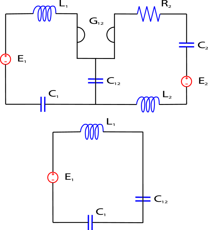
Figure 1: (Top) The electric circuit on top has a gryator $G_{12}$, three capacitances $C_{1}$, $C_{2}$, $C_{12}$, two inductances $L_{1}$, $L_{2}$, a resistor $R_{2}$, and two sources $E_{1}$, $E_{2}$. This electric circuit example fits within the framework of our model. Indeed, the resistor $R_{2}$ represents losses, the gyrator $G_{12}$ represents gyroscopy, and this two component system consists of a lossy component and a lossless component – the right and left circuits, respectively. (Bottom) The electric circuit on the bottom is obtained from the circuit above by eliminating in it the right circuit with lossy component $R_{2}$. This elimination corresponds to imposing constraint $q_{2}=0$ on the Lagrangian defined by equation (63). This bottom circuit has inductance $L_{1}$ and two capacitances $C_{1}$, $C_{12}$ connected in series to a source $E_{1}$. The frequencies of the eigenmodes of this circuit are $\rho_{3}$ and $\rho_{4}$ which are the limits of $\operatorname{Re}\zeta_{3}\left(\beta\right)$ and $\operatorname{Re}\zeta_{4}\left(\beta\right)$ [see the asymptotic expansions in (92)], the frequencies of the underdamped eigenmodes of the circuit above, as $\beta=\frac{R_{2}}{\ell}\rightarrow+\infty$, i.e., as losses in the lossy component (top right circuit) become infinite, as predicted by our theory on the selective overdamping phenomenon (see Fig. 5 and Remark 12 for more details on these results for this electric circuit example and Section 4.2, Proposition 23 and Remarks 22, 24 for more details on the general theory).

2.1 Lagrangian system

To derive evolution equations for the electric circuit with a gyrator in Fig. 1 we use a general method for constructing Lagrangians for circuits, [Gant, Sec. 9], that yields

$$\mathcal{L} =\mathcal{T}-\mathcal{V}\text{ \ \ \ \ \ \ \ \ \ \ \ \ \ \ \ (circuit Lagrangian),}$$ (63)

$$\mathcal{T} =\frac{L_{1}}{2}\dot{q}_{1}^{2}+\frac{L_{2}}{2}\dot{q}_{2}^{2}+\frac{G_{12}}{4}(q_{1}\dot{q}_{2}-\dot{q}_{1}q_{2}),\quad$$

$$\mathcal{V} =\frac{1}{2C_{1}}q_{1}^{2}+\frac{1}{2C_{12}}\left(q_{1}-q_{2}\right)^{2}+\frac{1}{2C_{2}}q_{2}^{2}-\frac{G_{12}}{4}(q_{1}\dot{q}_{2}-\dot{q}_{1}q_{2}),$$

$$\mathcal{R} =\frac{R_{2}}{2}\dot{q}_{2}^{2},$$

where $\mathcal{L}$ is the Lagrangian, $\mathcal{R}$ is the Rayleigh dissipative function, and $I_{1}=\dot{q}_{1}$, $I_{2}=\dot{q}_{2}$ are the currents. The sources we take to be zero, i.e., $E_{1}=E_{2}=0$. The general Euler-Lagrange equations of motion with forces are

$$\frac{\partial}{\partial t}\frac{\partial\mathcal{L}}{\partial\dot{Q}}-\frac{\partial\mathcal{L}}{\partial Q}=-\frac{\partial\mathcal{R}}{\partial\dot{Q}},$$ (64)

where $Q$ are the charges

$$Q=\left[\begin{array}[c]{c}q_{1}\\ q_{2}\end{array}\right],$$ (65)

yielding from (62)–(65) the following second-order ODEs

$$\alpha\ddot{Q}+\left(2\theta+\beta R\right)\dot{Q}+\eta Q=0,$$ (66)

with the dimensionless loss parameter

$$\beta=\frac{R_{2}}{\ell}\qquad\text{(where }\ell>0\text{ is fixed and has same units as }R_{2}\text{)}$$ (67)

that scales the intensity of losses in the system, and

$$\alpha=\left[\begin{array}[c]{cc}L_{1}&0\\ 0&L_{2}\end{array}\right],\qquad\eta=\left[\begin{array}[c]{cc}\frac{1}{C_{1}}+\frac{1}{C_{12}}&-\frac{1}{C_{12}}\\ -\frac{1}{C_{12}}&\frac{1}{C_{2}}+\frac{1}{C_{12}}\end{array}\right],$$ (72)

$$\theta=\left[\begin{array}[c]{cc}0&-\frac{G_{12}}{2}\\ \frac{G_{12}}{2}&0\end{array}\right],\qquad R=\left[\begin{array}[c]{cc}0&0\\ 0&\ell\end{array}\right].$$ (77)

Recall, the loss fraction $\delta_{R}$ defined in (17) is the ratio of the rank of the matrix $R$ to the total degrees of freedom $N$ of the system which in this case is

$$\text{loss fraction:\quad}\delta_{R}=\frac{N_{R}}{N}=\frac{1}{2},\qquad N=2,\qquad N_{R}=\operatorname{rank}R=1.$$ (78)

Thus, the Lagrangian system (66) fits with our framework described in Sec. 1.1 with the loss fraction condition (18), satisfied, i.e., $0<\delta_{R}<1$, and hence is a model of a two-component composite with a lossy and a lossless component.

2.2 Modal dichotomy and overdamping

We now will describe the modal dichotomy and overdamping phenomenon for this electric circuit following our discussion in Section 1.4.

First, the duality condition 27 holds in this example as

$$\eta>0$$ (79)

and so the equations of motion for the dual Lagrangian system are

$$\eta\ddot{Q}+\left(2\theta+\beta R\right)\dot{Q}+\alpha Q=0.$$ (80)

We now begin by calculating the spectra $\sigma\left(\alpha^{-1}R\right)$ and $\sigma\left(\eta^{-1}R\right)$ in order to calculate $b_{\min}$ and $b_{\min}^{\flat}$ in (26) and (29), respectively:

$$\sigma\left(\alpha^{-1}R\right) =\left\{b_{0},b_{1}\right\},\text{ }b_{0}=0,\text{ }b_{\min}=b_{1}=\ell L_{2}^{-1},$$ (81)

$$\sigma\left(\eta^{-1}R\right) =\left\{b_{0}^{\flat},b_{1}^{\flat}\right\},\text{ }b_{0}^{\flat}=0,\text{ }b_{\min}^{\flat}=b_{1}^{\flat}=\ell\left(\frac{1}{C_{2}}+\frac{1}{C_{1}+C_{12}}\right)^{-1}.$$ (82)

Next, we calculate $\omega_{\max}$, $\omega_{\min}$, and $\omega_{\max}^{\flat}$ in (24), (25), and (28), respectively, from the spectrum of the pencil

$$C\left(\zeta,\beta\right)=\zeta^{2}\alpha+\left(2\theta+\beta R\right)\mathrm{i}\zeta-\eta,$$

at $\beta=0$, i.e.,

$$\sigma\left(C\left(\cdot,0\right)\right)=\left\{\zeta\in\mathbb{C}:\det\left(\zeta^{2}\alpha\mathbf{+}2\zeta\mathrm{i}\theta-\eta\right)=0\right\}=\left\{\pm\omega_{\min},\pm\omega_{\max}\right\},$$

where

$$0<\omega_{\min}\leq\omega_{\max},$$

$$\omega_{\max}=\sqrt{\frac{a}{2}+\sqrt{\left(\frac{a}{2}\right)^{2}-\left(\det\alpha\right)^{-1}\det\eta}},$$

$$\omega_{\min}=\frac{1}{\omega_{\max}^{\flat}}=\sqrt{\frac{a}{2}-\sqrt{\left(\frac{a}{2}\right)^{2}-\left(\det\alpha\right)^{-1}\det\eta}},$$

$$a=\left(\frac{1}{L_{2}C_{12}}+\frac{1}{L_{1}C_{12}}+\frac{1}{L_{2}C_{2}}+\frac{1}{L_{1}C_{1}}+\frac{G_{12}^{2}}{L_{1}L_{2}}\right),\text{ }$$

$$\left(\det\alpha\right)^{-1}\det\eta=\left(L_{1}L_{2}\right)^{-1}\left(\frac{1}{C_{1}C_{2}}+\frac{1}{C_{1}C_{12}}+\frac{1}{C_{2}C_{12}}\right).$$

Next, we calculate the spectra $\rho_{\min}$, $\rho_{\max}$, and $\rho_{\min}^{\flat}$ in (39)-(41), which following the Remark 9, can be computed using Proposition 23 as

$$\rho_{\min}=\min\left\{\rho\in(0,\infty):\det\left[\left(P_{R}^{\bot}\alpha^{-1}C\left(\rho,0\right)P_{R}^{\bot}\right)|_{\operatorname{Ker}R}\right]=0\right\},$$

$$\rho_{\max}=\max\left\{\rho\in(0,\infty):\det\left[\left(P_{R}^{\bot}\alpha^{-1}C\left(\rho,0\right)P_{R}^{\bot}\right)|_{\operatorname{Ker}R}\right]=0\right\},$$

$$\rho_{\min}^{\flat}=\rho_{\max}^{-1},$$

where $P_{R}^{\bot}$ is the orthogonal projection onto $\operatorname{Ker}R$ (the nullspace of $R$) and in this example,

$$P_{R}^{\bot}=\left[\begin{array}[c]{cc}1&0\\ 0&0\end{array}\right],\text{ }P_{R}^{\bot}C\left(\rho,0\right)P_{R}^{\bot}=\left[L_{1}\rho^{2}-\left(\frac{1}{C_{1}}+\frac{1}{C_{12}}\right)\right]P_{R}^{\bot},$$ (85)

$$\left\{\rho\in\mathbb{C}:\det\left[\left(P_{R}^{\bot}C\left(\rho,0\right)P_{R}^{\bot}\right)|_{\operatorname{Ker}R}\right]=0\right\}=\left\{\rho_{3},\rho_{4}\right\},$$

$$\rho_{3}=-\rho_{4}=\rho_{\min}=\rho_{\max}=\frac{1}{\rho_{\min}^{\flat}}=\sqrt{L_{1}^{-1}\left(\frac{1}{C_{1}}+\frac{1}{C_{12}}\right)}.$$ (86)

Remark 12 (limiting frequencies)

In accordance with our theory (see Section 4.2, Proposition 23, and Remarks 22, 24 for more details), the real numbers $\rho_{3},\rho_{4}$ are the frequencies of the eigenmodes of a conservative Lagrangian system with Euler-Lagrange equations

$$L_{1}\ddot{q}_{1}+\left(\frac{1}{C_{1}}+\frac{1}{C_{12}}\right)q_{1}=0$$

corresponding to the Lagrangian

$$\mathcal{L}_{\operatorname{Ker}R}=\mathcal{L}_{\operatorname{Ker}R}\left(q_{1},\dot{q}_{1}\right)=\frac{1}{2}\left[\begin{array}[c]{l}\dot{q}_{1}\\ q_{1}\end{array}\right]^{\mathrm{T}}\left[\begin{array}[c]{ll}L_{1}&0\\ 0&\frac{1}{C_{1}}+\frac{1}{C_{12}}\end{array}\right]\left[\begin{array}[c]{l}\dot{q}_{1}\\ q_{1}\end{array}\right].$$

In particular, this is the Lagrangian of the electric circuit on the bottom of Fig. 1 with inductance $L_{1}$ and two capacitances $C_{1}$, $C_{12}$ connected in series (with no source, i.e., $E_{1}=0$). Notice that this is the same Lagrangian for a $LC$-circuit with inductor $L_{1}$ and capacitor $\left(\frac{1}{C_{1}}+\frac{1}{C_{12}}\right)^{-1}$. This makes sense since it well-known in electric circuit theory that connecting two capacitors $C_{1}$ and $C_{12}$ in series is the same as having one capacitor $C$ which is the one-half of the harmonic mean of the two capacitors, i.e., $C=$ $\left(\frac{1}{C_{1}}+\frac{1}{C_{12}}\right)^{-1}$.

Next, as the nonzero eigenvalues of $\alpha^{-1}R$ and $\eta^{-1}R$ are simple then this implies the generic condition (36) is true for both the Lagrangian system (66) and its dual system (80). Thus, the terms (43)-(45) for the selective overdamping in this example are

$$\beta_{0} =\frac{2\omega_{\max}}{d},\text{ where }d=\min_{0\leq i,j\leq N_{R},i\not=j}\left|b_{i}-b_{j}\right|=b_{1},$$ (87)

$$\beta_{1} =\max\left\{\beta_{0},\frac{2\omega_{\max}^{\flat}}{d^{\flat}}\right\},\text{ where }d^{\flat}=\min_{0\leq i,j\leq N_{R},i\not=j}\left|b_{i}^{\flat}-b_{j}^{\flat}\right|=b_{1}^{\flat},$$ (88)

$$\beta_{2} =\max\left\{\min\left\{c^{-1}\left(\rho_{\min}/2\right),\left(c^{\flat}\right)^{-1}\left(\rho_{\min}^{\flat}/2\right)\right\},2\frac{\omega_{\max}}{b_{\min}},2\frac{\omega_{\max}^{\flat}}{b_{\min}^{\flat}}\right\},$$ (89)

where the functions $c^{-1}\left(y\right)$ and $\left(c^{\flat}\right)^{-1}\left(y\right)$ are defined in (31) and (33), respectively.

Finally, according to our theory, as $\beta\rightarrow\infty$ there are eigenmodes $Q_{j}=Q_{j}\left(t,\beta\right)=q_{j}\left(\beta\right)e^{-\mathrm{i}\zeta_{j}\left(\beta\right)t}$, $j=1,2,3,4$ of the Lagrangian system such that $\left[Q_{j},\partial_{t}Q_{j}\right]^{\mathrm{T}}$, $j=1,2,3,4$ is a basis for the phase space $\mathbb{V}\left(\beta\right)$, as defined in (36) for this Lagrangian system (66)-(72), and which split into two distinct classes

$$\text{high-loss}\text{: }Q_{1}(\beta);\text{ low-loss}\text{: }Q_{j}(\beta),\text{ }2\leq j\leq 4$$

with the asymptotic expansions:

$$\text{high-loss:}-\operatorname{Im}\zeta_{1}\left(\beta\right)=b_{1}\beta+O\left(\beta^{-1}\right),\text{ }\operatorname{Re}\zeta_{1}\left(\beta\right)=0,$$ (90)

$$\text{low-loss, low-Q:}-\operatorname{Im}\zeta_{2}\left(\beta\right)=\frac{1}{b_{1}^{\flat}}\beta^{-1}+O\left(\beta^{-3}\right),\text{ }\operatorname{Re}\zeta_{2}\left(\beta\right)=0,$$ (91)

$$\text{low-loss, high-Q:}-\operatorname{Im}\zeta_{j}\left(\beta\right)=d_{j}\beta^{-1}+O\left(\beta^{-3}\right),\text{ }\operatorname{Re}\zeta_{j}\left(\beta\right)=\rho_{j}+O\left(\beta^{-2}\right),$$ (92)

$$\text{(quality factor) }Q_{\zeta_{j}\left(\beta\right)}=\frac{\left|\rho_{j}\right|}{d_{j}}\beta+O\left(\beta^{-1}\right)\text{ , for }j=3,4,$$

where in this example

$$d_{3}=d_{4}=\frac{1}{2}\frac{G_{12}^{2}}{\ell L_{1}}+\frac{1}{2}\frac{1}{\ell}\frac{C_{1}}{\left(C_{1}+C_{12}\right)C_{12}},$$ (93)

and $b_{1}$, $b_{1}^{\flat}$, $\rho_{3}$, $\rho_{4}$ are already calculated above.

Therefore, for this electric circuit example, the four stages (i)-(iv) of the modal dichotomy as described in Sec. 1.4.1 occur for (i) $\beta>\frac{2\omega_{\max}}{b_{\min}}=\beta_{0}$; (ii) $\beta>\max\left\{\frac{2\omega_{\max}}{b_{\min}},\frac{2\omega_{\max}^{\flat}}{b_{\min}^{\flat}}\right\}=\beta_{1}$; (iii) $\beta>\max\left\{c^{-1}\left(\frac{\rho_{\min}}{2}\right),2\frac{\omega_{\max}^{\flat}}{b_{\min}^{\flat}}\right\}\geq\beta_{2}\geq\beta_{1}$; (iv) $\beta\gg 1$. Moreover, the three stages (i)-(iii) of overdamping as described in Sec. 1.4.2 occur for (i) $\beta>\beta_{0}$; (ii) $\beta>\beta_{1}$; (iii) $\beta>\beta_{2}$. In particular, for this example, the two stages (i), (ii) of selective overdamping correspond to the two stages (i), (ii) for the modal dichotomy, respectively.

Remark 13

The method used to calculate the $d_{j}$’s is found in Sec. 4.2. It is calculated similar to the example in [FigWel1, Sec. III] by using the formula in (261) below and the system operator $A\left(\beta\right)=\Omega-\mathrm{i}\beta B$ for the Lagrangian system (66) in this example.

Remark 14

Notice that for these lowest order terms only in the low-loss, high-Q modes, i.e., the underdamped modes, does gyroscopy effect the modes. And more precisely for the lowest order asympotics ($b_{1}$, $b_{1}^{\flat}$, $\rho_{j}$, $d_{j}$, $j=3,4$), gyroscopy has no effect on the frequencies $\operatorname{Re}\zeta_{j}\left(\beta\right)$, $j=1,2,3,4$ or damping factors of the overdamped modes $\operatorname{Im}\zeta_{j}\left(\beta\right)$, $j=1,2$, yet gyroscopy does have an effect on the damping factors of the underdamped modes $\operatorname{Im}\zeta_{j}\left(\beta\right)$, $j=3,4$. The effect is proportional to $G_{12}^{2}=\left\|2\theta\right\|^{2}$, where $\left\|\cdot\right\|$ denotes the operator norm. As the interplay between losses and gyroscopy in Lagrangian systems is of significant interest, it would be interesting to derive formulas for higher order terms for the frequencies and damping factors of the eigenmodes to see how gyroscopy effects these terms asymptotically as $\beta\rightarrow\infty$.

2.3 Numerical Analysis

We will now illustrate the behavior of the eigenmodes $Q_{j}\left(t,\beta\right)=q_{j}\left(\beta\right)e^{-\mathrm{i}\zeta_{j}\left(\beta\right)t}$, $j=1,2,3,4$ for the electric circuit with gyrator in Fig. 1 as a function of the loss parameter $\beta$ based on the theory described above and focusing on the overdamping phenomena and the asymptotic expansions (90)-(93) in the high-loss regime as $\beta\rightarrow\infty$:

high-loss $$\text{: }\zeta_{1}\left(\beta\right)=\zeta_{1}^{a}\left(\beta\right)+O\left(\beta^{-1}\right),\text{ }\zeta_{1}^{a}\left(\beta\right)=-\mathrm{i}b_{1}\beta,\text{ }\operatorname{Re}\zeta_{1}\left(\beta\right)=0,$$ (94)

low-loss, low-Q $$\text{: }\zeta_{2}\left(\beta\right)=\zeta_{2}^{a}\left(\beta\right)+O\left(\beta^{-3}\right),\text{ }\zeta_{2}^{a}\left(\beta\right)=-\mathrm{i}\frac{1}{b_{1}^{\flat}}\beta^{-1},\text{ }\operatorname{Re}\zeta_{2}\left(\beta\right)=0,$$ (95)

low-loss, high-Q $$\text{: }\zeta_{j}\left(\beta\right)=\zeta_{j}^{a}\left(\beta\right)+O\left(\beta^{-2}\right),\text{ }\zeta_{j}^{a}\left(\beta\right)=\rho_{j}-\mathrm{i}d_{j}\beta^{-1},\text{ \ }\operatorname{Re}\zeta_{j}\left(\beta\right)\not=0,$$ (96)

for $j=3,4$.

All the figures below were generated (by Marcus Marinho) with MATLAB${}^{\text{\textregistered}}$ using the framework described in Sec. 1.5 by just calculating the eigenvalues of the system operator $A\left(\beta\right)=\Omega-\mathrm{i}\beta B$, $\beta\geq 0$ (a $4\times 4$ matrix in this circuit example) since, according to our theory, they are the values $\zeta_{j}\left(\beta\right)$, $j=1,2,3,4$.

We fix positive values of the capacitance $C_{1}$, $C_{2}$, $C_{12}$, inductances $L_{1}$, $L_{2}$, gyration resistance $G_{12}/2$ (the term coined by Tellegen in [Tell48]), and $\ell$ [where the dimensionless loss parameter is $\beta=R_{2}/\ell$ in (67) with resistance $R_{2}>0$]. For the numerical analysis in this section, we choose

$$C_{1}=C_{2}=25,\text{ }C_{12}=\frac{25}{3},\text{ }L_{1}=10,\text{ }L_{2}=\frac{1}{2},\text{ }G_{12}=\frac{5}{2},\text{ }\ell=10.$$ (97)

The values of $\beta_{0}$, $\beta_{1}$, $\beta_{2}$ in Theorem 43, Corollary 44, and Corollary 35, respectively, where the high-loss modes are guaranteed to be overdamped for $\beta>\beta_{0}$, where the overdamped low-loss modes are guaranteed to be overdamped for $\beta>\beta_{1}$, and where the underdamped low-loss modes are guaranteed to be underdamped for $\beta>\beta_{2}$ are determined explicitly using the analysis in Sec. 2.1 which we calculate from Eqs. (87)-(89), using the values from (97), to be

$$\beta_{0} =\frac{2\omega_{\max}}{d}=\frac{2\omega_{\max}}{b_{\min}}=\frac{1}{1000}\sqrt{7930+10\sqrt{626609}}\approx 0.1258803552,$$ (98)

$$\beta_{1} =\max\left\{\beta_{0},\frac{2\omega_{\max}^{\flat}}{d^{\flat}}\right\}=\frac{2\omega_{\max}^{\flat}}{b_{\min}^{\flat}}=\frac{7}{5\sqrt{7930-10\sqrt{626609}}}\approx 0.3723591130,$$

$$\beta_{2} =\max\left\{\min\left\{c^{-1}\left(\rho_{\min}/2\right),\left(c^{\flat}\right)^{-1}\left(\rho_{\min}^{\flat}/2\right)\right\},2\frac{\omega_{\max}}{b_{\min}},2\frac{\omega_{\max}^{\flat}}{b_{\min}^{\flat}}\right\}=c^{-1}\left(\rho_{\min}/2\right)$$

$$=\frac{1}{20000}\left(7930+10\sqrt{626609}\right)\sqrt{10}+\frac{1}{1000}\sqrt{7930+10\sqrt{626609}}$$

$$\approx 2.631331413.$$

In the figures below (see Figs. 2-6), we give a graphical representation of the effects of increasing losses, i.e., increasing $\beta=\frac{R_{2}}{\ell}$ (with $\ell$ fixed), in the lossy component of the electric circuit with gyrator in Fig. 1 on frequencies $\operatorname{Re}\zeta_{j}\left(\beta\right)$, damping factors $-\operatorname{Im}\zeta_{j}\left(\beta\right)$, and quality factor $Q_{\zeta_{j}\left(\beta\right)}=\frac{1}{2}\frac{\left|\operatorname{Re}\zeta_{j}\left(\beta\right)\right|}{-\operatorname{Im}\zeta_{j}\left(\beta\right)}$ ($j=1,2,3,4$) of all the eigenmodes of the dissipative-gyroscopic Lagrangian system (66) [with the numerical values (97)].

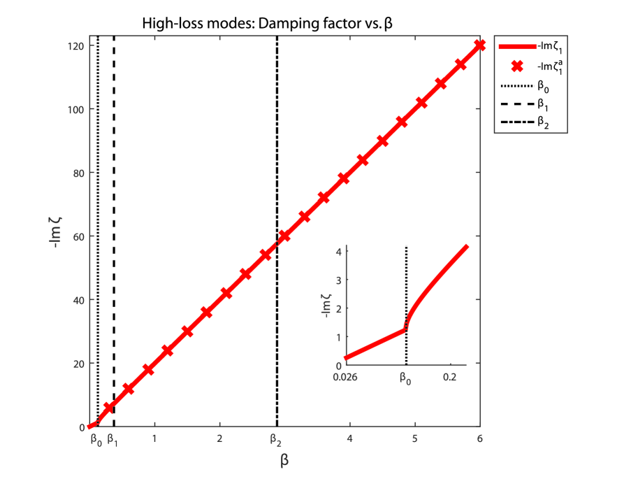
Figure 2: For the electric circuit with gyrator in Fig. 1 with the numerical values (97), the graph of damping factor $-\operatorname{Im}\zeta_{1}\left(\beta\right)$ of the high-loss eigenmodes with the asymptotic approximation $-\operatorname{Im}\zeta_{1}^{a}\left(\beta\right)=b_{1}\beta$ in (81) and (94) as a function of the loss parameter $\beta=\frac{R_{2}}{\ell}$ (with $\ell$ fixed). In the inset, a close-up of the damping factor in neighborhood of the value $\beta_{0}$ from Theorem 43 where the high-loss modes are guaranteed to be overdamped for $\beta>\beta_{0}$.

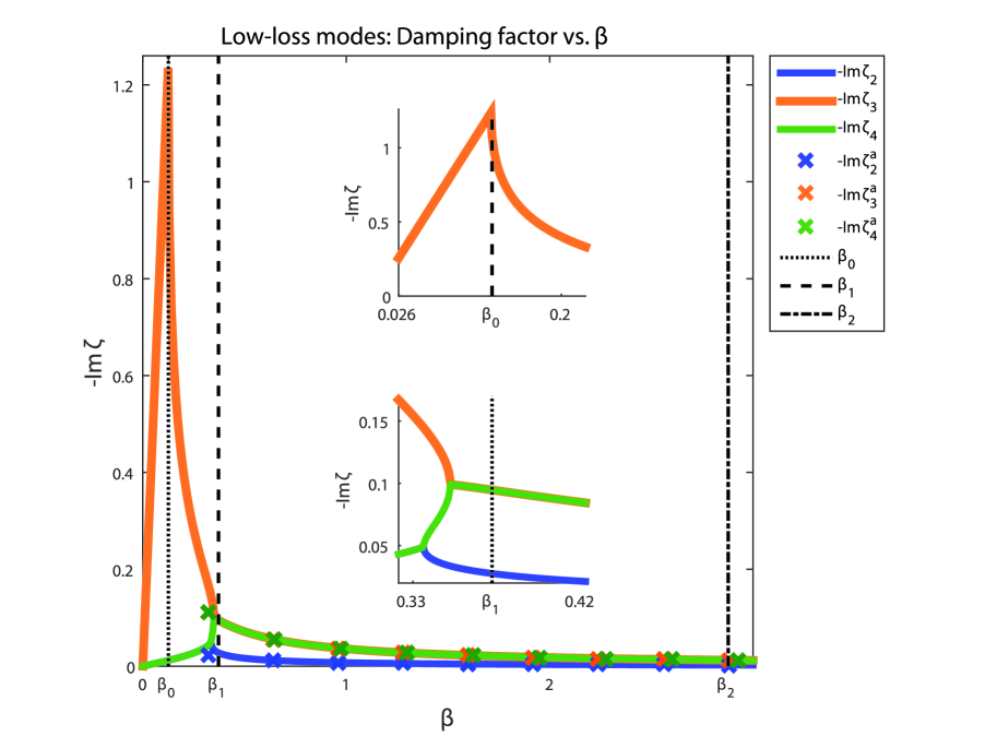
Figure 3: For the electric circuit with gyrator in Fig. 1 with the numerical values (97), the graph of damping factors $-\operatorname{Im}\zeta_{j}\left(\beta\right)$, $j=2,3,4$ of the low-loss eigenmodes with the asymptotic approximation $-\operatorname{Im}\zeta_{2}^{a}\left(\beta\right)=\frac{1}{b_{1}^{\flat}}\beta^{-1}$ in (82) and (95) and $-\operatorname{Im}\zeta_{j}^{a}\left(\beta\right)=d_{j}\beta^{-1}$ in (93) and (96) for $j=3,4$, as a function of the loss parameter $\beta=\frac{R_{2}}{\ell}$ (with $\ell$ fixed). Due to the spectral symmetry described in Proposition 20, we always have $\left\{\zeta_{1}\left(\beta\right),\zeta_{2}\left(\beta\right),\zeta_{3}\left(\beta\right),\zeta_{4}\left(\beta\right)\right\}=\left\{-\overline{\zeta_{1}\left(\beta\right)},-\overline{\zeta_{2}\left(\beta\right)},-\overline{\zeta_{3}\left(\beta\right)},-\overline{\zeta_{4}\left(\beta\right)}\right\}$ and so there can be intervals where the damping factors overlap, as seen in this figure. In the bottom inset, a close-up of the damping factor in neighborhood of the value $\beta_{1}$ from Corollary 44 where the overdamped low-loss modes, with damping factor $-\operatorname{Im}\zeta_{2}\left(\beta\right)$ shown as the blue curve, are guaranteed to be overdamped for $\beta>\beta_{1}$. Comparing this figure and the insets with that of Fig. 2, one can see clearly the modal dichotomy near $\beta=\beta_{0}$, between the high-loss modes with damping factor $-\operatorname{Im}\zeta_{1}\left(\beta\right)$ and the low-loss modes with damping factors $-\operatorname{Im}\zeta_{j}\left(\beta\right)$, $j=2,3,4$ (as described by Theorem 26 and Corollary 27) and near $\beta=\beta_{1}$, between the low-loss, low-Q modes with damping factor $-\operatorname{Im}\zeta_{2}\left(\beta\right)$ and the low-loss mode, high-Q modes with damping factors $-\operatorname{Im}\zeta_{j}\left(\beta\right)$, $j=3,4$ (as described by Theorem 28 and Corollary 29).

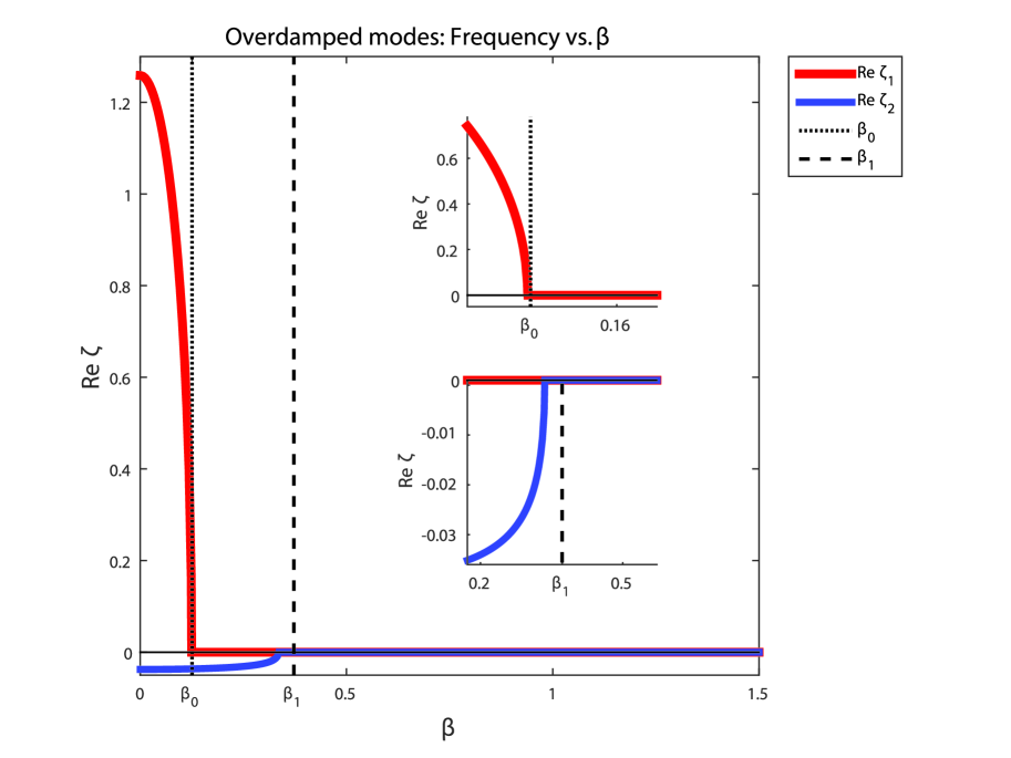
Figure 4: For the electric circuit with gyrator in Fig. 1 with the numerical values (97), the graph of frequencies $\operatorname{Re}\zeta_{j}\left(\beta\right)$, $j=1,2$ of the overdamped eigenmodes as a function of the loss parameter $\beta=\frac{R_{2}}{\ell}$ (with $\ell$ fixed). In the top inset, a close-up of the frequency in neighborhood of the value $\beta_{0}$ from Theorem 43 where the high-loss modes, with frequency $\operatorname{Re}\zeta_{1}\left(\beta\right)$ shown as the red curve, are guaranteed to be overdamped for $\beta>\beta_{0}$. This overdamping is clearly visible since $\operatorname{Re}\zeta_{1}\left(\beta\right)=0$ for $\beta>\beta_{0}$ in this figure. In the bottom inset, a close-up of the frequencies in neighborhood of the value $\beta_{1}$ from Corollary 44 where the overdamped low-loss modes, with frequency $\operatorname{Re}\zeta_{2}\left(\beta\right)$ shown as the blue curve, are guaranteed to be overdamped for $\beta>\beta_{1}$. This overdamping is clearly visible since $\operatorname{Re}\zeta_{2}\left(\beta\right)=0$ for $\beta>\beta_{1}$ in this figure.

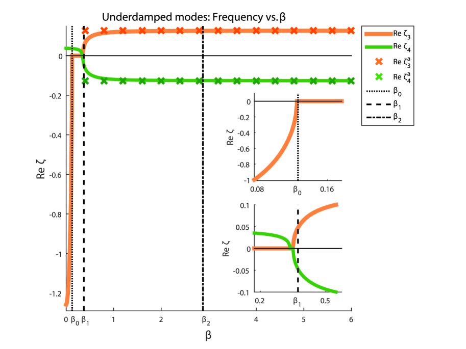
Figure 5: For the electric circuit with gyrator in Fig. 1 with the numerical values (97), the graph of frequencies $\operatorname{Re}\zeta_{j}\left(\beta\right)$, $j=3,4$ of the low-loss, high-Q eigenmodes with the asymptotic approximation $\operatorname{Re}\zeta_{j}^{a}\left(\beta\right)=\rho_{j}$, $j=3,4$ in (86) and (96) as a function of the loss parameter $\beta$. The low-loss, high-Q eigenmodes are guaranteed to be underdamped for $\beta>\beta_{2}$ by Corollary 35, that is, $\operatorname{Re}\zeta_{j}\left(\beta\right)\not=0$ for $j=3,4$ as this figure indicates. Although outside the scope of our studies here, it is interesting to point out some other interesting phenomena which can be seen in these figures. For instance, in regards to the low-loss eigenmodes, i.e., those with frequencies $\operatorname{Re}\zeta_{j}\left(\beta\right)$, $j=2,3,4$, there can be open intervals in $(\beta_{0},\beta_{1})$ where some of the frequencies are identically zero such as for $\operatorname{Re}\zeta_{3}\left(\beta\right)$ near $\beta=\beta_{0}$ (see top inset). And there is even an interval $\mathcal{I}\subseteq(\beta_{0},\beta_{1})$, near $\beta=\beta_{1}$, where all the eigenmode of the system have their frequencies identically zero, i.e., $\operatorname{Re}\zeta_{j}\left(\beta\right)\equiv 0$, $j=1,2,3,4$ (see bottom insets in this figure and in Fig. 4).

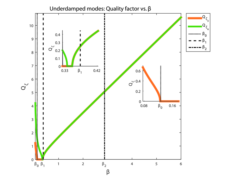
Figure 6: For the electric circuit with gyrator in Fig. 1 with the numerical values (97), the graph of quality factors (Q-factor) $Q_{\zeta_{j}\left(\beta\right)}=\frac{1}{2}\frac{\left|\operatorname{Re}\zeta_{j}\left(\beta\right)\right|}{-\operatorname{Im}\zeta_{j}\left(\beta\right)}$, $j=3,4$ of the low-loss, high-Q eigenmodes as a function of the loss parameter $\beta$. These eigenmodes are guaranteed to be underdamped for $\beta>\beta_{2}$ (by Corollary 35) and estimates on their dissipative properties in terms of the modal dichotomy is described in Theorem 33 and Corollary 34. In particular, according to our theory $Q_{\zeta_{j}\left(\beta\right)}\nearrow+\infty$ (i.e., increases without bound) as $\beta\rightarrow\infty$ (see Corollary 34), which this figure indicates. Due to the spectral symmetry described in Proposition 20 and Theorem 28 [see (211)], we must have $\left\{\zeta_{3}\left(\beta\right),\zeta_{4}\left(\beta\right)\right\}=\left\{-\overline{\zeta_{3}\left(\beta\right)},-\overline{\zeta_{4}\left(\beta\right)}\right\}$ for $\beta>\beta_{1}$. This offers an explaination as to why we have intervals in which $Q_{\zeta_{3}\left(\beta\right)}=Q_{\zeta_{4}\left(\beta\right)}$ in this figure since in those intervals $\zeta_{4}\left(\beta\right)=-\overline{\zeta_{3}\left(\beta\right)}$. In fact, this is guaranteed to be true for $\beta>\beta_{2}$ by Theorem 28 [see (211)] and Corollary 35.

3 The Lagrangian system and its dual

In this paper, a linear Lagrangian system will be a system whose state is described by a time-dependent $Q=Q(t)$ taking values in the Hilbert space $\mathbb{C}^{N}$ with the standard inner product $(\cdot,\cdot)$ (i.e., $(a,b)=a^{\ast}b$, where $\ast$ denotes the conjugate transpose, i.e., $a^{\ast}=\overline{a}^{\mathrm{T}}$) whose dynamics are governed by the ODEs (1). And associated with this system is its Lagrangian $\mathcal{L}$ in (11) and its Rayleigh dissipation function $\mathcal{R}$ in (12).

3.1 Dual system

To the Lagrangian $\mathcal{L}$ (11) there is a corresponding ”dual” Lagrangian $\mathcal{L}^{\flat}$ defined by

$$\mathcal{L}^{\flat}=\mathcal{L}^{\flat}\left(Q,\dot{Q}\right)=-\mathcal{L}\left(\dot{Q},Q\right)=$$ (99)

$$=\frac{1}{2}\left[\begin{array}[c]{l}\dot{Q}\\ Q\end{array}\right]^{\mathrm{T}}\left[\begin{array}[c]{ll}\eta&\theta\\ \theta^{\mathrm{T}}&-\alpha\end{array}\right]\left[\begin{array}[c]{l}\dot{Q}\\ Q\end{array}\right]\qquad\text{(dual Lagrangian).}$$ (106)

From the definition of the dual, a fundamental property is $\left(\mathcal{L}^{\flat}\right)^{\flat}=$ $\mathcal{L}$.

The general Euler-Lagrange equations of motion for the Lagrangian system with Lagrangian $\mathcal{L}^{\flat}$ and Rayleigh dissipation function $\mathcal{R}$ in (12) is

$$\eta\ddot{Q}+\left(2\theta+\beta R\right)\dot{Q}+\alpha Q=0\qquad\text{(evolution equations for the dual system).}$$ (107)

This linear Lagrangian system, whose states have dynamics governed by the ODEs (107), will be called the dual Lagrangian system. This system is obtained from our original Lagrangian system (1) by just making the substitution $\left(\alpha,\eta\right)\longmapsto\left(\eta,\alpha\right)$. In particular, this means whenever $\eta^{-1}$ exists, the dual Lagrangian $\mathcal{L}^{\flat}$ has all the same assumptions satisfied as our Lagrangian $\mathcal{L}$ as well including the duality condition (27) being true. Therefore, whenever the duality condition (27) is true, i.e., $\eta>0$, then all results in this paper that apply to the Lagrangian system (1) will also apply to it’s dual Lagrangian system (107). The importance of this duality will become clear when we study the modal dichotomy and overdamping phenomena.

We will also need to introduce the following notation convention.

Notation 15

In the rest of this paper, whenever we use the superscript notation $X^{\flat}$ it will be implicitly understood that $X$ is an associated with the Lagrangian system and $X^{\flat}$ is the same object but associated with dual Lagrangian system, e.g., the dual Lagrangian $\mathcal{L}^{\flat}$, dual Hamiltonian $\mathcal{H}^{\flat}$, dual quadratic matrix pencil $C^{\flat}\left(\zeta,\beta\right)$, dual system operator $A^{\flat}\left(\beta\right)=\Omega^{\flat}-\mathrm{i}\beta B^{\flat}$, etc.

Using this notation, the system energy for the dual Lagrangian system, which has the Lagrangian $\mathcal{L}^{\flat}$ in (99), can be calculated in terms of the definition in (15) of $\mathcal{V}$, $\mathcal{T}$ of the Lagrangian system (1) by:

$$\mathcal{L}^{\flat}=\mathcal{T}^{\flat}-\mathcal{V}^{\flat},\qquad 0\leq\mathcal{H}^{\flat}=\mathcal{T}^{\flat}\mathcal{+V}^{\flat}\text{ \ \ \ (dual Hamiltonian),}$$ (108)

$$\mathcal{T}^{\flat}=\mathcal{V}(Q,\dot{Q}),\qquad\mathcal{V}^{\flat}=\mathcal{T}(Q,\dot{Q})\text{.}$$

Also from our definition and notation we have the Rayleigh dissipation functions are the same, i.e.,

$$\mathcal{R}^{\flat}=\mathcal{R}\qquad\text{(dual Rayleigh dissipation function).}$$ (109)

On the eigenmodes and the quality factor of the dual system. Given an eigenmode $Q(t)=qe^{-\mathrm{i}\zeta t}$ (with $\zeta\not=0$) of the Lagrangian system (1) it follows that $Q^{\flat}(t)=qe^{-\mathrm{i}\left(-\zeta^{-1}\right)t}$ is an eigenmode of the dual Lagrangian system (107) since

$$0=\eta\ddot{Q}+\left(2\theta+\beta R\right)\dot{Q}+\alpha Q=\left(-\mathrm{i}\zeta\right)^{2}\left(\eta\ddot{Q}^{\flat}+\left(2\theta+\beta R\right)\dot{Q}^{\flat}+\alpha Q^{\flat}\right).$$ (110)

For each eigenmode $Q$ with nonzero eigenfrequency $\zeta$, we will refer to $Q^{\flat}$ as it’s dual eigenmode. With this definition, it follows that the quality factor $Q_{\zeta}$ of the eigenmode of the Lagrangian system (1) is exactly the quality factor $Q_{-\zeta^{-1}}$ of this dual eigenmode of the dual Lagrangian system (107) since by the definition of the quality factor in (21) we have

$$Q_{-\zeta^{-1}}=-\frac{1}{2}\frac{\left|\operatorname{Re}\left(-\zeta^{-1}\right)\right|}{\operatorname{Im}\left(-\zeta^{-1}\right)}=-\frac{1}{2}\frac{\left|\operatorname{Re}\zeta\right|}{\operatorname{Im}\zeta}=Q_{\zeta}\qquad\text{(equivalence of the Q-factors).}$$ (111)

3.2 Standard versus pencil formulations of the spectral problems

In this section we elaborate on the relationship between the two main spectral problems in this paper, namely, between the standard eigenvalue problem (59) for the system operator $A\left(\beta\right)=\Omega-\mathrm{i}\beta B$ and the quadratic eigenvalue problem (46) for the quadratic matrix pencil $C\left(\zeta,\beta\right)$. We will also describe some spectral properties of the system operator $A\left(\beta\right)$ and that of the dual system operator $A^{\flat}\left(\beta\right)$. The results in this section are need for our main results in Sec. 4 on the modal dichotomy and overdamping phenomena.

First, we begin with some notation. The Hilbert space $H=\mathbb{C}^{2N}$ with standard inner product $\left(\cdot,\cdot\right)$ can be decomposed as $H=H_{\mathrm{p}}\oplus H_{\mathrm{q}}$ into the orthogonal subspaces $H_{\mathrm{p}}=\mathbb{C}^{N}$, $H_{\mathrm{q}}=\mathbb{C}^{N}$ with orthogonal matrix projections

$$P_{\mathrm{p}}=\left[\begin{array}[c]{cc}\mathbf{1}&0\\ 0&0\end{array}\right],\qquad P_{\mathrm{q}}=\left[\begin{array}[c]{cc}0&0\\ 0&\mathbf{1}\end{array}\right].$$ (112)

In particular, the matrix $A\left(\beta\right)$ defined in (51), (57) is a block matrix already partitioned with respect to the decomposition $H=H_{\mathrm{p}}\oplus H_{\mathrm{q}}$ and any vector $w\in H$ can be represented uniquely in the block form

$$w=\left[\begin{array}[c]{c}\varphi\\ \psi\end{array}\right],\qquad\text{where }\varphi=P_{\mathrm{p}}w,\qquad\psi=P_{\mathrm{q}}w.$$ (113)

With respect to this decomposition, we have the following results from [FigWel2]. First, the following proposition tells us the characteristic matrix of the system operator $\zeta\mathbf{1}-A\left(\beta\right)$ can be factored in terms of the quadratic matrix pencil $C\left(\zeta,\beta\right)$. Second, the corollary that follows gives the description of the spectral equivalence between the two main spectral problems (46) and (59).

Proposition 16

If $\zeta\not=0$ then

$$\zeta\mathbf{1}-A\left(\beta\right)=$$ (114)

$$=\left[\begin{array}[c]{cc}K_{\mathrm{p}}&\zeta^{-1}\mathrm{i}\Phi^{\mathrm{T}}\\ 0&\mathbf{1}\end{array}\right]\left[\begin{array}[c]{cc}\zeta^{-1}\mathbf{1}&0\\ 0&\zeta\mathbf{1}\end{array}\right]\left[\begin{array}[c]{cc}C(\zeta,\beta)&0\\ 0&\mathbf{1}\end{array}\right]\left[\begin{array}[c]{cc}K_{\mathrm{p}}^{\mathrm{T}}&0\\ -\zeta^{-1}\mathrm{i}\Phi&\mathbf{1}\end{array}\right].$$ (123)

Corollary 17 (spectral equivalence)

For any $\zeta\in\mathbb{C}$,

$$\det\left(\zeta\mathbf{1}-A\left(\beta\right)\right)=\frac{\det C(\zeta,\beta)}{\det\alpha}.$$ (124)

In particular, the system operator $A\left(\beta\right)$ and quadratic matrix pencil $C(\zeta,\beta)$ have the same spectrum, i.e.,

$$\sigma\left(A\left(\beta\right)\right)=\sigma\left(C\left(\cdot,\beta\right)\right).$$ (125)

Moreover, if $\zeta\not=0$ then the following statements are true:

1. If $A\left(\beta\right)w=\zeta w$ and $w\not=0$ then

   $$w=\left[\begin{array}[c]{c}-\mathrm{i}\zeta\sqrt{\alpha}q\\ \sqrt{\eta}q\end{array}\right],\qquad\text{where }C(\zeta,\beta)q=0,\qquad q\not=0.$$ (126)

2. If $C(\zeta,\beta)q=0$ and $q\not=0$ then

   $$A\left(\beta\right)w=\zeta w\text{,}\qquad\text{where }w=\left[\begin{array}[c]{c}-\mathrm{i}\zeta\sqrt{\alpha}q\\ \sqrt{\eta}q\end{array}\right]\not=0.$$ (127)

The following lemma tells us that the eigenvalues of the system operator $A\left(\beta\right)$ are nonzero whenever the duality condition (27) is true and so the eigenvectors will have the unique block representation in Corollary 17.

Lemma 18

If (27) is true then $\Omega$ is invertible and $A\left(\beta\right)$ is invertible. In particular, $0\not\in\sigma\left(A\left(\beta\right)\right)$.

Proof. Suppose (27) is true, i.e., $\eta$ is invertible. Then $K$, as defined in (49) is invertible and hence $\Omega=\mathrm{i}KJK^{\mathrm{T}}$ is invertible, where $J\,$ is the invertible $2N\times 2N$ symplectic matrix $J=\begin{bmatrix}0&-\mathbf{1}\\ \mathbf{1}&0\end{bmatrix}$. Next, if $A\left(\beta\right)w=0$ then $\Omega w=-\mathrm{i}\beta Bw$ which implies $\left(w,\Omega w\right)=-\mathrm{i}\beta\left(w,Bw\right)$. But since $\Omega^{\ast}=\Omega$, $B^{\ast}=B$, and $\beta$ is real this implies $\left(w,Bw\right)=0$ and since $B\geq 0$ this implies $Bw=0$ which implies $\Omega w=0$. And since $\Omega$ was shown to be invertible then $w=0$ and so $0\not\in\sigma\left(A\left(\beta\right)\right)$. This completes the proof.   

Whenever the duality condition (27) is true, the dual Lagrangian system (107) with (dual) system operator $A^{\flat}\left(\beta\right)$ has the corresponding (dual) quadratic matrix pencil

$$C^{\flat}(\zeta,\beta)=\zeta^{2}\eta+\left(2\theta+\beta R\right)\mathrm{i}\zeta-\alpha\qquad\text{(dual quadratic pencil).}$$ (128)

The following proposition describes the correspondence between the standard eigenvalue problem (59) for the system operator $A\left(\beta\right)$ and that of the dual system operator $A^{\flat}\left(\beta\right)$.

Proposition 19 (spectral equivalence-duality)

Suppose (27) is true. Then the following statements are true:

1. For any $\zeta\not=0$,

   $$C(\zeta,\beta) =-\zeta^{2}C^{\flat}(-\zeta^{-1},\beta),$$

   $$\det\left(\zeta\mathbf{1}-A\left(\beta\right)\right) =\frac{\left(-\zeta^{2}\right)^{N}\det\eta}{\det\alpha}\det\left(\left(-\zeta^{-1}\right)\mathbf{1}-A^{\flat}\left(\beta\right)\right)$$ (129)

   $$=\left(-1\right)^{N}\det\left(\left(-\zeta\right)\mathbf{1}-\left[A^{\flat}\left(\beta\right)\right]^{-1}\right).$$

2. The system operator $A\left(\beta\right)$ is related to the spectrum of dual system operator $A^{\flat}\left(\beta\right)$ by

   $$\sigma\left(A\left(\beta\right)\right)=-\sigma\left(A^{\flat}\left(\beta\right)\right)^{-1}.$$ (130)

3. If $\zeta$ is an eigenvalue of $A\left(\beta\right)$ then $-\zeta^{-1}$ is an eigenvalue of $A^{\flat}\left(\beta\right)$ and they have the same geometric multiplicity, algebraic multiplicity, and partial multiplicities (i.e., for the corresponding eigenvalue they have the same Jordan normal form).

4. If $\zeta$, $w$ is an eigenpair of the system operator $A\left(\beta\right)$ then $-\zeta^{-1}$, $w^{\flat}$ is an eigenpair of the dual system operator $A^{\flat}\left(\beta\right)$, where

   $$w=\left[\begin{array}[c]{c}-\mathrm{i}\zeta\sqrt{\alpha}q\\ \sqrt{\eta}q\end{array}\right],\qquad w^{\flat}=\left[\begin{array}[c]{c}-\mathrm{i}\left(-\zeta^{-1}\right)\sqrt{\eta}q\\ \sqrt{\alpha}q\end{array}\right],$$ (135)

   $$C(\zeta,\beta)q=0,\text{ }C^{\flat}(-\zeta^{-1},\beta)q=0,\text{\ \ }q\not=0.$$

Proof. First, if $\zeta\not=0$ then by Corollary 17 and duality we have

$$C(\zeta,\beta)=\zeta^{2}\alpha+\left(2\theta+\beta R\right)\mathrm{i}\zeta-\eta$$

$$=-\zeta^{2}\left(-\alpha+\left(2\theta+\beta R\right)\mathrm{i}\left(-\zeta^{-1}\right)+\left(-\zeta^{-1}\right)^{2}\eta\right)=-\zeta^{2}C^{\flat}(-\zeta^{-1},\beta),$$

$$\det\left(\zeta\mathbf{1}-A\left(\beta\right)\right)=\frac{\det C(\zeta,\beta)}{\det\alpha}=\frac{\left(-\zeta^{2}\right)^{N}\det\eta}{\det\alpha}\frac{\det C^{\flat}(-\zeta^{-1},\beta)}{\det\eta}$$

$$=\frac{\left(-\zeta^{2}\right)^{N}\det\eta}{\det\alpha}\det\left(\left(-\zeta^{-1}\right)\mathbf{1}-A^{\flat}\left(\beta\right)\right)$$

$$=\frac{\left(-1\right)^{N}\det\eta}{\det\alpha}\det\left[A^{\flat}\left(\beta\right)\right]\det\left(\left(-\zeta\right)\mathbf{1}-\left[A^{\flat}\left(\beta\right)\right]^{-1}\right)$$

$$=\left(-1\right)^{N}\det\left(\left(-\zeta\right)\mathbf{1}-\left[A^{\flat}\left(\beta\right)\right]^{-1}\right).$$

It then follows immediately from this and Lemma 18 that

$$\sigma\left(A\left(\beta\right)\right)=-\sigma\left(A^{\flat}\left(\beta\right)\right)^{-1}.$$

Next, it follows from Corollary 17 and Lemma 18 that if $\zeta$, $w$ is an eigenpair of the system operator $A\left(\beta\right)$ then $\zeta\not=0$ and

$$w=\left[\begin{array}[c]{c}-\mathrm{i}\zeta\sqrt{\alpha}q\\ \sqrt{\eta}q\end{array}\right],\qquad C(\zeta,\beta)q=0,\text{\ \ }q\not=0.$$

But this implies that

$$C^{\flat}(-\zeta^{-1},\beta)q=\left(-\zeta^{2}\right)^{-1}C(\zeta,\beta)q=0,\qquad q\not=0$$

implying by Corollary 17 and duality that $-\zeta^{-1}$, $w^{\flat}$ is an eigenpair of the dual system operator $A^{\flat}\left(\beta\right)$ with

$$w^{\flat}=\left[\begin{array}[c]{c}-\mathrm{i}\left(-\zeta^{-1}\right)\sqrt{\eta}q\\ \sqrt{\alpha}q\end{array}\right].$$

This proves statements 1, 2, and 4. Finally, statement 3 follows immediately from statement 1 and Lemma 18. This completes the proof.   

The next proposition from [FigWel2] describes the spectral symmetries of the system operator $A\left(\beta\right)$ which follows from its fundamental property (52).

Proposition 20 (spectral symmetry)

The following statements are true:

1. The characteristic polynomial of $A\left(\beta\right)$ satisfies

   $$\overline{\det\left(-\overline{\zeta}\mathbf{1}-A\left(\beta\right)\right)}=\det\left(\zeta I-A\left(\beta\right)\right),$$ (136)

   for every $\zeta\in\mathbb{C}$.  In particular, the spectrum $\sigma\left(A\left(\beta\right)\right)$ of the system operator $A\left(\beta\right)$ is symmetric with respect to the imaginary axis of the complex plane, i.e.,

   $$\sigma\left(A\left(\beta\right)\right)=-\overline{\sigma\left(A\left(\beta\right)\right)}\text{.}$$ (137)

2. If $w$ is an eigenvector of the system operator $A\left(\beta\right)$ with corresponding eigenvalue $\zeta$ then $\overline{w}$ is an eigenvector of $A$ with corresponding eigenvalue $-\overline{\zeta}$.

The next proposition in this section relates the spectrum of matrices $\Omega$, $B$ in the definition of the system operator $A\left(\beta\right)=\Omega-\mathrm{i}\beta B$ and the spectrum of the matrices $\Omega^{\flat}$, $B^{\flat}$ for the dual system operator $A^{\flat}\left(\beta\right)=\Omega^{\flat}-\mathrm{i}\beta B^{\flat}$ to the matrices $\alpha$, $\eta$, $\theta$, $R$.

Proposition 21 (spectra relations I)

For the $2N\times 2N$ matrices $B$, $\Omega$ and the $N\times N$ matrices $\alpha$, $\eta$, $\theta$, $R$ we have

$$\det\left(\zeta\mathbf{1}-\Omega\right) =\left(\det\alpha\right)^{-1}\det C\left(\zeta,0\right)=\left(\det\alpha\right)^{-1}\det\left(\zeta^{2}\alpha+2\theta\mathrm{i}\zeta-\eta\right),$$ (138)

$$\det\left(\zeta\mathbf{1}-B\right) =\zeta^{N}\det\left(\zeta\alpha-R\right),$$

for every $\zeta\in\mathbb{C}$ and

$$\sigma\left(\Omega\right)=\sigma\left(C\left(\cdot,0\right)\right)\subseteq\mathbb{R},\text{\quad}\sigma\left(\Omega\right)=-\sigma\left(\Omega\right),\text{\quad}\sigma\left(B\right)\setminus\left\{0\right\}=\sigma\left(\alpha^{-1}R\right)\setminus\left\{0\right\}.$$ (139)

In particular, if $b_{\min}$ and $\omega_{\max}$ denote the smallest nonzero eigenvalue and the largest eigenvalue of $B$ and $\Omega$, respectively, then

$$b_{\min}=\min\left[\sigma\left(\alpha^{-1}R\right)\setminus\left\{0\right\}\right],\qquad\omega_{\max}=\left\|\Omega\right\|=\max\sigma\left(C\left(\cdot,0\right)\right).$$ (140)

Moreover, if (27) is true then

$$\sigma\left(\Omega^{\flat}\right)=-\sigma\left(\Omega\right)^{-1}=\sigma\left(\Omega^{-1}\right),\qquad\sigma\left(B^{\flat}\right)\setminus\left\{0\right\}=\sigma\left(\eta^{-1}R\right)\setminus\left\{0\right\}.$$ (141)

In particular, if $b_{\text{min}}^{\flat}$ and $\omega_{\text{max}}^{\flat}$ denote the smallest nonzero eigenvalue and the largest eigenvalue of $B^{\flat}$ and $\Omega^{\flat}$, respectively, then

$$b_{\min}^{\flat}=\min\left[\sigma\left(\eta^{-1}R\right)\setminus\left\{0\right\}\right],\qquad\omega_{\max}^{\flat}=\left\|\Omega^{\flat}\right\|=\left\|\Omega^{-1}\right\|=\omega_{\min}^{-1},$$ (142)

where

$$\omega_{\min}=\min\left|\sigma\left(\Omega\right)\right|$$ (143)

is the smallest positive eigenvalue of $\Omega$.

Proof. It follows by Corollary 17 that

$$\det\left(\zeta\mathbf{1}-\Omega\right)=\det\left(\zeta\mathbf{1}-A\left(0\right)\right)=$$

$$=\left(\det\alpha\right)^{-1}\det C\left(\zeta,0\right)=\left(\det\alpha\right)^{-1}\det\left(\zeta^{2}\alpha+2\theta\mathrm{i}\zeta-\eta\right)$$

and it follows immediately from the definition of $B$ that

$$\det\left(\zeta\mathbf{1}-B\right)=\zeta^{N}\det\left(\zeta\alpha-R\right)=\zeta^{N}\left(\det\alpha\right)\det\left(\zeta\mathbf{1}-\alpha^{-1}R\right)$$

for every $\zeta\in\mathbb{C}$. Now the $2N\times 2N$ matrices $\Omega$, $B$ have the fundamental properties

$$\Omega=\Omega^{\ast}=-\Omega^{\mathrm{T}},\qquad\text{ }B\geq 0,$$

from which it follows that

$$\sigma\left(\Omega\right)=\sigma\left(C\left(\cdot,0\right)\right)\subseteq\mathbb{R},\qquad\sigma\left(\Omega\right)=-\sigma\left(\Omega\right),$$

$$\sigma\left(B\right)\setminus\left\{0\right\}=\sigma\left(\alpha^{-1}R\right)\setminus\left\{0\right\},$$

and

$$b_{\min}=\min\left[\sigma\left(\alpha^{-1}R\right)\setminus\left\{0\right\}\right],$$

$$\omega_{\max}=\left\|\Omega\right\|=\max\left|\sigma\left(\Omega\right)\right|=\max\left|\sigma\left(\Omega\right)\right|=\max\sigma\left(C\left(\cdot,0\right)\right).$$

Suppose now that (27) is true. Then from what we just proved we have

$$\sigma\left(B^{\flat}\right)\setminus\left\{0\right\}=\sigma\left(\eta^{-1}R\right)\setminus\left\{0\right\},$$

and

$$\omega_{\max}^{\flat}=\left\|\Omega^{\flat}\right\|.$$

In particular,

$$b_{\min}^{\flat}=\min\left[\sigma\left(\eta^{-1}R\right)\setminus\left\{0\right\}\right].$$

By Proposition 19 we have

$$\sigma\left(\Omega^{\flat}\right)=\sigma\left(A^{\flat}\left(0\right)\right)=-\sigma\left(A\left(0\right)\right)^{-1}=-\sigma\left(\Omega\right)^{-1}.$$

Then since $\sigma\left(\Omega\right)=-\sigma\left(\Omega\right)$ this together with Lemma 18 implies

$$\sigma\left(\Omega^{\flat}\right)=-\sigma\left(\Omega\right)^{-1}=\sigma\left(\Omega^{-1}\right).$$

From which it follows that

$$\omega_{\text{max}}^{\flat}=\left\|\Omega^{\flat}\right\|=\left\|\Omega^{-1}\right\|=\left(\min\left|\sigma\left(\Omega\right)\right|\right)^{-1}.$$

But since $\sigma\left(\Omega\right)=-\sigma\left(\Omega\right)$ then

$$\min\left|\sigma\left(\Omega\right)\right|=\min\sigma\left(\Omega\right)=\omega_{\min}$$

is the smallest positive eigenvalue of $\Omega$. This completes the proof.   

Remark 22 (limiting frequencies)

This final proposition and the remark that follows, describes the spectrum of an important self-adjoint operator $\Omega_{1}$ on $\operatorname{Ker}B$ that plays a key role in the high-loss regime $\beta\gg 1$ in describing the modal dichotomy in Sec. 4.1 and in describing the spectral asymptotics of $A\left(\beta\right)$ as $\beta\rightarrow\infty$ in Sec. 4.2. In particular, if $\rho_{j}$, $j=N_{R}+1,\ldots,2N$ are all the eigenvalues of $\Omega_{1}$ (repeated according to their multiplicities as eigenvalues of $\Omega_{1}$) then in the perturbation analysis of the frequencies $\operatorname{Re}\zeta_{j}\left(\beta\right)$, $j=N_{R}+1,\ldots,2N$ of the low-loss eigenmodes, as described in Sec. 4.2 [see (262)], we have the limiting frequencies:

$$\lim_{\beta\rightarrow\infty}\operatorname{Re}\zeta_{j}\left(\beta\right)=\rho_{j}\text{, for }j=N_{R}+1,\ldots,2N;\text{ \ \ }\sigma\left(\Omega_{1}\right)=\left\{\rho_{j}:N_{R}+1\leq j\leq 2N\right\}.$$ (144)

Proposition 23 (spectral relations II)

Let $P_{B}^{\bot}$ denote the orthogonal projection of the Hilbert space $\mathbb{C}^{2N}$, with standard inner product $\left(\cdot,\cdot\right)$, onto $\operatorname{Ker}B$ (i.e., the nullspace of $B$). Denote by $\Omega_{1}=\left.P_{B}^{\bot}\Omega P_{B}^{\bot}\right|_{\operatorname{Ker}B}:\operatorname{Ker}B\rightarrow\operatorname{Ker}B$ the restriction of $P_{B}^{\bot}\Omega P_{B}^{\bot}$ to $\operatorname{Ker}B$. For any operator $M$ on a finite dimensional vector space over $\mathbb{C}$, we will denote the product of its eigenvalues (counting multiplicities) by $\det M$. Then the matrix $P_{B}^{\bot}\Omega P_{B}^{\bot}\not=0$ if and only if $N_{R}<N$ (i.e., $R$ is rank deficient), and in this case the following statements are true:

1. The nonzero eigenvalues of $P_{B}^{\bot}\Omega P_{B}^{\bot}$ are real and come in $\pm$ pairs with equal multiplicity. In particular,

   $$0\in\sigma\left(P_{B}^{\bot}\Omega P_{B}^{\bot}\right)=-\sigma\left(P_{B}^{\bot}\Omega P_{B}^{\bot}\right)\subseteq\mathbb{R}.$$ (145)

2. The operator $\Omega_{1}$ is self-adjoint with respect to the inner product $\left(\cdot,\cdot\right)$ and for every $\rho\in\mathbb{C}$,

   $$\det\left(\rho\mathbf{1}-\Omega_{1}\right)=\rho^{N_{R}}\frac{\det\left[\left.P_{R}^{\bot}C\left(\rho,0\right)P_{R}^{\bot}\right|_{\operatorname{Ker}R}\right]}{\det\left(\left.P_{R}^{\bot}\alpha P_{R}^{\bot}\right|_{\operatorname{Ker}R}\right)}$$ (146)

   where $P_{R}^{\bot}$ denotes the orthogonal projection onto $\operatorname{Ker}R$,

   $$\left.P_{R}^{\bot}C\left(\rho,0\right)P_{R}^{\bot}\right|_{\operatorname{Ker}R} :\operatorname{Ker}R\rightarrow\operatorname{Ker}R,$$ (147)

   $$\left.P_{R}^{\bot}\alpha P_{R}^{\bot}\right|_{\operatorname{Ker}R} :\operatorname{Ker}R\rightarrow\operatorname{Ker}R,$$ (148)

   are the restriction of $P_{R}^{\bot}C\left(\rho,0\right)P_{R}^{\bot}$ and $P_{R}^{\bot}\alpha P_{R}^{\bot}$ to $\operatorname{Ker}R$, and $\left.P_{R}^{\bot}\alpha P_{R}^{\bot}\right|_{\operatorname{Ker}R}$ is invertible. In particular,

   $$\sigma\left(P_{B}^{\bot}\Omega P_{B}^{\bot}\right)=\sigma\left(\Omega_{1}\right)=\left\{\rho\in\mathbb{C}:\det\left[\left.P_{R}^{\bot}C\left(\rho,0\right)P_{R}^{\bot}\right|_{\operatorname{Ker}R}\right]=0\right\}\cup\left\{0\right\}.$$ (149)

3. If $\rho_{0}\not=0$ is an eigenvalue of $P_{B}^{\bot}\Omega P_{B}^{\bot}$ then its multiplicity is equal to the multiplicity as an eigenvalue of $\Omega_{1}$ which is equal to the order of the zero of the polynomial (of degree $2N-2N_{R}$) $\det\left[\left.P_{R}^{\bot}C\left(\rho,0\right)P_{R}^{\bot}\right|_{\operatorname{Ker}R}\right]$ at $\rho=\rho_{0}$.

4. The eigenvalue $0$ of $\Omega_{1}$ has multiplicity $N_{R}$ if and only if $\operatorname{Ker}R\cap\operatorname{Ker}\eta=\left\{0\right\}$, in which case

   $$\dim\operatorname{Ker}\left(\Omega_{1}\right)=N_{R}\text{, }\dim\operatorname{Ran}\left(P_{B}^{\bot}\Omega P_{B}^{\bot}\right)=\dim\operatorname{Ran}\left(\Omega_{1}\right)=2\left(N-N_{R}\right).$$ (150)

5. If (27) is true then, denoting the corresponding dual operator of $\Omega_{1}$ for the dual Lagrangian system (107) by $\Omega_{1}^{\flat}$, the following are true: i) $0$ is an eigenvalue of both $\Omega_{1}^{\flat}$ and $\Omega_{1}$ of equal multiplicity $N_{R}$; (iii) $\left.P_{R}^{\bot}C\left(\rho,0\right)P_{R}^{\bot}\right|_{\operatorname{Ker}R}=-\rho^{2}\left.P_{R}^{\bot}C^{\flat}\left(-\rho^{-1},0\right)P_{R}^{\bot}\right|_{\operatorname{Ker}R}$ for $\rho\not=0$; (iv) $\rho\not=0$ is an eigenvalue of $\Omega_{1}$ of multiplicity $m$ if and only $-\rho^{-1}$ is an eigenvalue of $\Omega_{1}^{\flat}$ of multiplicity $m$. In particular, if we define $\rho_{\min}$ and $\rho_{\max}$ by

   $$\rho_{\min}=\min\left[\sigma\left(\Omega_{1}\right)\cap\left(0,\infty\right)\right],\text{ }\rho_{\max}=\max\sigma\left(\Omega_{1}\right),$$

   and letting $\rho_{\min}^{\flat}$, $\rho_{\max}^{\flat}$ denote these corresponding values for the dual Lagrangian system (107) then

   $$\rho_{\min}^{\flat}=\rho_{\max}^{-1}\text{, }\rho_{\max}^{\flat}=\rho_{\min}^{-1}.$$

Proof. Suppose that $P_{B}^{\bot}\Omega P_{B}^{\bot}\not=0$. From block matrix representation of $B$ and $\Omega$ in (57) with respect to the decomposition $\mathbb{C}^{2N}=\mathbb{C}^{N}\oplus\mathbb{C}^{N}$, it follows that $P_{B}^{\bot}$, $P_{B}^{\bot}\Omega P_{B}^{\bot}$ have the block matrix representation

$$P_{B}^{\bot}=\left[\begin{array}[c]{ll}P_{\mathsf{\tilde{R}}}^{\bot}&0\\ 0&\mathbf{1}\end{array}\right],\text{ }P_{B}^{\bot}\Omega P_{B}^{\bot}=\mathrm{i}\begin{bmatrix}-2P_{\mathsf{\tilde{R}}}^{\bot}\sqrt{\alpha}^{-1}\theta\sqrt{\alpha}^{-1}P_{\mathsf{\tilde{R}}}^{\bot}&-P_{\mathsf{\tilde{R}}}^{\bot}\sqrt{\alpha}^{-1}\sqrt{\eta}\\ \sqrt{\eta}\sqrt{\alpha}^{-1}P_{\mathsf{\tilde{R}}}^{\bot}&0\end{bmatrix},$$ (151)

where $\mathbf{1}$ denotes the identity operator on $\mathbb{C}^{N}$, $P_{\mathsf{\tilde{R}}}^{\bot}$ denotes the orthogonal projection onto $\operatorname{Ker}\mathsf{\tilde{R}}$, and $\mathsf{\tilde{R}}=K_{\mathrm{p}}RK_{\mathrm{p}}^{\mathrm{T}}$ with $K_{\mathrm{p}}=\sqrt{\alpha}^{-1}$. Also, as $B=B^{\ast}=B^{\mathrm{T}}$ this implies $P_{B}^{\bot}=\left(P_{B}^{\bot}\right)^{\ast}=\left(P_{B}^{\bot}\right)^{\mathrm{T}}$ so that since $\Omega=\Omega^{\ast}=-\Omega^{\mathrm{T}}$ then

$$P_{B}^{\bot}\Omega P_{B}^{\bot}=\left(P_{B}^{\bot}\Omega P_{B}^{\bot}\right)^{\ast}=-\left(P_{B}^{\bot}\Omega P_{B}^{\bot}\right)^{\mathrm{T}}.$$

From these facts we have, $0$ is an eigenvalue of $P_{B}^{\bot}\Omega P_{B}^{\bot}$ and it’s nonzero eigenvalues are real and come in $\pm$ pairs with equal multiplicity. In particular,

$$0\in\sigma\left(P_{B}^{\bot}\Omega P_{B}^{\bot}\right)=-\sigma\left(P_{B}^{\bot}\Omega P_{B}^{\bot}\right)\subseteq\mathbb{R}\text{.}$$

It also follows immediately that $\Omega_{1}$ is self-adjoint with respect to the inner product $\left(\cdot,\cdot\right)$ since $P_{B}^{\bot}\Omega P_{B}^{\bot}$ is.

Next, we will prove the operator identity $\sqrt{\alpha}^{-1}P_{\mathsf{\tilde{R}}}^{\bot}\sqrt{\alpha}^{-1}=P_{R}^{\bot}\sqrt{\alpha}^{-1}P_{\mathsf{\tilde{R}}}^{\bot}\sqrt{\alpha}^{-1}P_{R}^{\bot}$, where $P_{R}^{\bot}$ denotes the orthogonal projection onto $\operatorname{Ker}R$. First, since $P_{\mathsf{\tilde{R}}}^{\bot}$ and $P_{R}^{\bot}$ are orthogonal projections onto $\operatorname{Ker}\mathsf{\tilde{R}}$ and $\operatorname{Ker}R$ for the real symmetric matrices $\mathsf{\tilde{R}}$ and $R$, respectively, then $\left(P_{\mathsf{\tilde{R}}}^{\bot}\right)^{2}=P_{\mathsf{\tilde{R}}}^{\bot}=\left(P_{\mathsf{\tilde{R}}}^{\bot}\right)^{\ast}$, $\left(P_{R}^{\bot}\right)^{2}=P_{R}^{\bot}=\left(P_{R}^{\bot}\right)$, $\operatorname{Ran}P_{\mathsf{\tilde{R}}}^{\bot}=\operatorname{Ker}\mathsf{\tilde{R}}$ $=\sqrt{\alpha}\operatorname{Ker}R$, $\operatorname{Ker}P_{\mathsf{\tilde{R}}}^{\bot}=\operatorname{Ran}\mathsf{\tilde{R}}$ $=\left(\operatorname{Ker}\mathsf{\tilde{R}}\right)^{\bot}=\sqrt{\alpha}^{-1}\operatorname{Ran}R$, $\operatorname{Ran}P_{R}^{\bot}=\operatorname{Ker}R$, and $\operatorname{Ker}P_{R}^{\bot}=\operatorname{Ran}R=\left(\operatorname{Ker}R\right)^{\bot}$. These facts imply that $P_{R}^{\bot}\sqrt{\alpha}^{-1}P_{\mathsf{\tilde{R}}}^{\bot}=\sqrt{\alpha}^{-1}P_{\mathsf{\tilde{R}}}^{\bot}$ and so by taking complex conjugate transpose we have $P_{\mathsf{\tilde{R}}}^{\bot}\sqrt{\alpha}^{-1}P_{R}^{\bot}=P_{\mathsf{\tilde{R}}}^{\bot}\sqrt{\alpha}^{-1}$. This implies $\sqrt{\alpha}^{-1}P_{\mathsf{\tilde{R}}}^{\bot}\sqrt{\alpha}^{-1}=P_{R}^{\bot}\sqrt{\alpha}^{-1}P_{\mathsf{\tilde{R}}}^{\bot}\sqrt{\alpha}^{-1}=\sqrt{\alpha}^{-1}P_{\mathsf{\tilde{R}}}^{\bot}\sqrt{\alpha}^{-1}P_{R}^{\bot}$. Multiply this identity by $P_{R}^{\bot}$ on the left implies that $\sqrt{\alpha}^{-1}P_{\mathsf{\tilde{R}}}^{\bot}\sqrt{\alpha}^{-1}=P_{R}^{\bot}\sqrt{\alpha}^{-1}P_{\mathsf{\tilde{R}}}^{\bot}\sqrt{\alpha}^{-1}P_{R}^{\bot}$, which is the desired identity.

Next, it follows from this and the fact that $\sqrt{\alpha}^{-1}:\operatorname{Ker}\mathsf{\tilde{R}}\rightarrow\operatorname{Ker}R$ is an invertible map with inverse $\sqrt{\alpha}:\operatorname{Ker}R\rightarrow\operatorname{Ker}\mathsf{\tilde{R}}$ with that

$$P_{\mathsf{\tilde{R}}}^{\bot}K_{\mathrm{p}}C\left(\rho,0\right)K_{\mathrm{p}}^{\mathrm{T}}P_{\mathsf{\tilde{R}}}^{\bot}=\left(P_{\mathsf{\tilde{R}}}^{\bot}\sqrt{\alpha}^{-1}C\left(\rho,0\right)\sqrt{\alpha}^{-1}P_{\mathsf{\tilde{R}}}^{\bot}\right)$$

$$=P_{\mathsf{\tilde{R}}}^{\bot}\sqrt{\alpha}^{-1}P_{R}^{\bot}C\left(\rho,0\right)P_{R}^{\bot}\sqrt{\alpha}^{-1}P_{\mathsf{\tilde{R}}}^{\bot}=P_{\mathsf{\tilde{R}}}^{\bot}\sqrt{\alpha}^{-1}P_{R}^{\bot}\left(P_{R}^{\bot}C\left(\rho,0\right)P_{R}^{\bot}\right)|_{\operatorname{Ker}R}P_{R}^{\bot}\sqrt{\alpha}^{-1}P_{\mathsf{\tilde{R}}}^{\bot}$$

where $\left(P_{R}^{\bot}C\left(\rho,0\right)P_{R}^{\bot}\right)|_{\operatorname{Ker}R}$ is the restrictions of $P_{R}^{\bot}C\left(\rho,0\right)P_{R}^{\bot}$ to $\operatorname{Ker}R$.

We will now prove that $\sqrt{\alpha}^{-1}P_{\mathsf{\tilde{R}}}^{\bot}\sqrt{\alpha}^{-1}:\operatorname{Ker}R\rightarrow\operatorname{Ker}R$ is invertible with inverse $P_{R}^{\bot}\alpha P_{R}^{\bot}:\operatorname{Ker}R\rightarrow\operatorname{Ker}R$. First, $\sqrt{\alpha}^{-1}:\operatorname{Ker}\mathsf{\tilde{R}}\rightarrow\operatorname{Ker}R$ is an invertible map with inverse $\sqrt{\alpha}:\operatorname{Ker}R\rightarrow\operatorname{Ker}\mathsf{\tilde{R}}$. Second, we have

$$\operatorname{rank}\left(\sqrt{\alpha}^{-1}P_{\mathsf{\tilde{R}}}^{\bot}\sqrt{\alpha}^{-1}\right) =\operatorname{rank}P_{\mathsf{\tilde{R}}}^{\bot}=\dim\operatorname{Ran}P_{\mathsf{\tilde{R}}}^{\bot}=\dim\left(\operatorname{Ker}\mathsf{\tilde{R}}\right)$$

$$=\dim\left(\sqrt{\alpha}\operatorname{Ker}R\right)=\dim\operatorname{Ker}R.$$

It follows immediately from this that $\sqrt{\alpha}^{-1}P_{\mathsf{\tilde{R}}}^{\bot}\sqrt{\alpha}^{-1}:\operatorname{Ker}R\rightarrow:\operatorname{Ker}R$ is invertible. Next, it follows that $P_{\mathsf{\tilde{R}}}^{\bot}\sqrt{\alpha}P_{R}^{\bot}=\sqrt{\alpha}P_{R}^{\bot}$, since $\operatorname{Ran}P_{\mathsf{\tilde{R}}}^{\bot}=\operatorname{Ker}\mathsf{\tilde{R}}$ $=\sqrt{\alpha}\operatorname{Ker}R=\operatorname{Ran}\sqrt{\alpha}P_{R}^{\bot}$ and $\mathbb{C}^{N}=\operatorname{Ran}P_{R}^{\bot}\oplus\operatorname{Ker}P_{R}^{\bot}$, and hence taking the complex conjugate transpose yields $P_{R}^{\bot}\sqrt{\alpha}P_{\mathsf{\tilde{R}}}^{\bot}=$ $P_{R}^{\bot}\sqrt{\alpha}$ so that together with the fact that $P_{R}^{\bot}\sqrt{\alpha}^{-1}P_{\mathsf{\tilde{R}}}^{\bot}=\sqrt{\alpha}^{-1}P_{\mathsf{\tilde{R}}}^{\bot}$ we have

$$P_{R}^{\bot}\alpha P_{R}^{\bot}\sqrt{\alpha}^{-1}P_{\mathsf{\tilde{R}}}^{\bot}\sqrt{\alpha}^{-1}=P_{R}^{\bot}\alpha\left(\sqrt{\alpha}^{-1}P_{\mathsf{\tilde{R}}}^{\bot}\right)\sqrt{\alpha}^{-1}$$

$$=P_{R}^{\bot}\sqrt{\alpha}P_{\mathsf{\tilde{R}}}^{\bot}\sqrt{\alpha}^{-1}=\left(P_{R}^{\bot}\sqrt{\alpha}\right)\sqrt{\alpha}^{-1}=P_{R}^{\bot},$$

which implies the inverse of $\sqrt{\alpha}^{-1}P_{\mathsf{\tilde{R}}}^{\bot}\sqrt{\alpha}^{-1}:\operatorname{Ker}R\rightarrow:\operatorname{Ker}R$ is $P_{R}^{\bot}\alpha P_{R}^{\bot}:\operatorname{Ker}R\rightarrow\operatorname{Ker}R$.

Now suppose $\rho\not=0$. Then by the block representations of $\rho\mathbf{1}-A\left(0\right)$ and $P_{B}^{\bot}$ in Proposition 16 and (151), we have

$$\left[\begin{array}[c]{cc}P_{R}^{\bot}\alpha P_{R}^{\bot}\sqrt{\alpha}^{-1}P_{\mathsf{\tilde{R}}}^{\bot}&0\\ -\rho^{-1}\mathrm{i}\Phi P_{\mathsf{\tilde{R}}}^{\bot}&\mathbf{1}\end{array}\right]=\left[\begin{array}[c]{cc}P_{R}^{\bot}\alpha\sqrt{\alpha}^{-1}P_{\mathsf{\tilde{R}}}^{\bot}&0\\ -\rho^{-1}\mathrm{i}\Phi P_{\mathsf{\tilde{R}}}^{\bot}&\mathbf{1}\end{array}\right]$$ (156)

$$=\left[\begin{array}[c]{cc}P_{R}^{\bot}\sqrt{\alpha}P_{\mathsf{\tilde{R}}}^{\bot}&0\\ 0&\mathbf{1}\end{array}\right]\left[\begin{array}[c]{cc}\mathbf{1}&0\\ -\rho^{-1}\mathrm{i}\Phi P_{\mathsf{\tilde{R}}}^{\bot}&\mathbf{1}\end{array}\right]$$ (161)

and so defining

$$X =\left[\begin{array}[c]{cc}\mathbf{1}&\rho^{-1}\mathrm{i}P_{\mathsf{\tilde{R}}}^{\bot}\Phi^{\mathrm{T}}\\ 0&\mathbf{1}\end{array}\right]\left[\begin{array}[c]{cc}P_{\mathsf{\tilde{R}}}^{\bot}\sqrt{\alpha}^{-1}P_{R}^{\bot}&0\\ 0&\mathbf{1}\end{array}\right],\text{ }$$ (166)

$$Y =\left[\begin{array}[c]{cc}P_{R}^{\bot}\sqrt{\alpha}P_{\mathsf{\tilde{R}}}^{\bot}&0\\ 0&\mathbf{1}\end{array}\right]\left[\begin{array}[c]{cc}\mathbf{1}&0\\ -\rho^{-1}\mathrm{i}\Phi P_{\mathsf{\tilde{R}}}^{\bot}&\mathbf{1}\end{array}\right],$$ (171)

we have

$$\rho P_{B}^{\bot}-P_{B}^{\bot}\Omega P_{B}^{\bot}=P_{B}^{\bot}\left[\rho\mathbf{1}-A\left(0\right)\right]P_{B}^{\bot}=$$ (172)

$$=\left[\begin{array}[c]{cc}P_{\mathsf{\tilde{R}}}^{\bot}&\rho^{-1}\mathrm{i}P_{\mathsf{\tilde{R}}}^{\bot}\Phi^{\mathrm{T}}\\ 0&\mathbf{1}\end{array}\right]\left[\begin{array}[c]{cc}\rho^{-1}P_{\mathsf{\tilde{R}}}^{\bot}&0\\ 0&\rho\mathbf{1}\end{array}\right]$$ (177)

$$\times\left[\begin{array}[c]{cc}P_{\mathsf{\tilde{R}}}^{\bot}K_{\mathrm{p}}C\left(\rho,0\right)K_{\mathrm{p}}^{\mathrm{T}}P_{\mathsf{\tilde{R}}}^{\bot}&0\\ 0&\mathbf{1}\end{array}\right]\left[\begin{array}[c]{cc}P_{\mathsf{\tilde{R}}}^{\bot}&0\\ -\rho^{-1}\mathrm{i}\Phi P_{\mathsf{\tilde{R}}}^{\bot}&\mathbf{1}\end{array}\right]$$ (182)

$$=X\left[\begin{array}[c]{cc}\rho^{-1}P_{R}^{\bot}&0\\ 0&\rho\mathbf{1}\end{array}\right]\left[\begin{array}[c]{cc}\left(P_{R}^{\bot}C\left(\rho,0\right)P_{R}^{\bot}\right)|_{\operatorname{Ker}R}\left.P_{R}^{\bot}\alpha P_{R}^{\bot}\right|_{\operatorname{Ker}R}^{-1}&0\\ 0&\mathbf{1}\end{array}\right]Y,$$ (187)

where the operator $P_{R}^{\bot}\sqrt{\alpha}^{-1}P_{\mathsf{\tilde{R}}}^{\bot}:\operatorname{Ker}\mathsf{\tilde{R}}\rightarrow\operatorname{Ker}R$ is invertible whose inverse is the operator $P_{\mathsf{\tilde{R}}}^{\bot}\sqrt{\alpha}P_{R}^{\bot}:\operatorname{Ker}R\rightarrow\operatorname{Ker}\mathsf{\tilde{R}}$. The latter facts follow from facts that

$$P_{R}^{\bot}\sqrt{\alpha}^{-1}P_{\mathsf{\tilde{R}}}^{\bot}\left(P_{\mathsf{\tilde{R}}}^{\bot}\sqrt{\alpha}P_{R}^{\bot}\right) =P_{R}^{\bot}\sqrt{\alpha}^{-1}\left(P_{\mathsf{\tilde{R}}}^{\bot}\sqrt{\alpha}P_{R}^{\bot}\right)=P_{R}^{\bot}\sqrt{\alpha}^{-1}\sqrt{\alpha}P_{R}^{\bot}=P_{R}^{\bot},$$

$$\left(P_{\mathsf{\tilde{R}}}^{\bot}\sqrt{\alpha}P_{R}^{\bot}\right)P_{R}^{\bot}\sqrt{\alpha}^{-1}P_{\mathsf{\tilde{R}}}^{\bot} =P_{\mathsf{\tilde{R}}}^{\bot}\sqrt{\alpha}\left(P_{R}^{\bot}\sqrt{\alpha}^{-1}P_{\mathsf{\tilde{R}}}^{\bot}\right)=P_{\mathsf{\tilde{R}}}^{\bot}\sqrt{\alpha}\sqrt{\alpha}^{-1}P_{\mathsf{\tilde{R}}}^{\bot}=P_{\mathsf{\tilde{R}}}^{\bot},$$

which follow from the facts $P_{R}^{\bot}$ and $P_{\mathsf{\tilde{R}}}^{\bot}$ are projections onto $\operatorname{Ker}R$ and $\operatorname{Ker}\mathsf{\tilde{R}}$, respectively, together with identities $P_{\mathsf{\tilde{R}}}^{\bot}\sqrt{\alpha}P_{R}^{\bot}=\sqrt{\alpha}P_{R}^{\bot}$ and $P_{R}^{\bot}\sqrt{\alpha}^{-1}P_{\mathsf{\tilde{R}}}^{\bot}=\sqrt{\alpha}^{-1}P_{\mathsf{\tilde{R}}}^{\bot}$. It follows immediately, from the identities (172), (166) and the fact that $P_{R}^{\bot}\sqrt{\alpha}^{-1}P_{\mathsf{\tilde{R}}}^{\bot}:\operatorname{Ker}\mathsf{\tilde{R}}\rightarrow\operatorname{Ker}R$ and $P_{\mathsf{\tilde{R}}}^{\bot}\sqrt{\alpha}P_{R}^{\bot}:\operatorname{Ker}R\rightarrow\operatorname{Ker}\mathsf{\tilde{R}}$ are inverses of each other, that for all $\rho\in\mathbb{C},$

$$\det\left(\rho\mathbf{1}-\Omega_{1}\right) =\rho^{N_{R}}\det\left[\left.P_{R}^{\bot}C\left(\rho,0\right)P_{R}^{\bot}\right|_{\operatorname{Ker}R}\left.P_{R}^{\bot}\alpha P_{R}^{\bot}\right|_{\operatorname{Ker}R}^{-1}\right]$$

$$=\rho^{N_{R}}\frac{\det\left[\left.P_{R}^{\bot}C\left(\rho,0\right)P_{R}^{\bot}\right|_{\operatorname{Ker}R}\right]}{\det\left(\left.P_{R}^{\bot}\alpha P_{R}^{\bot}\right|_{\operatorname{Ker}R}\right)}.$$

In particular, this implies that if $\rho_{0}\not=0$ then $\rho=\rho_{0}$ is an eigenvalue of $\Omega_{1}$ of multiplicity $m$ if and only if $\rho=\rho_{0}$ is a zero of $\det\left[\left(P_{R}^{\bot}C\left(\rho,0\right)P_{R}^{\bot}\right)|_{\operatorname{Ker}R}\right]$ of multiplicity $m$. And $\rho=0$ is an eigenvalue of $\Omega_{1}$ of multiplicity $m$ if and only if $\rho=0$ is a zero of $\det\left[\left(P_{R}^{\bot}C\left(\rho,0\right)P_{R}^{\bot}\right)|_{\operatorname{Ker}R}\right]$ of multiplicity $m-N_{R}\geq 0$. This proves the first three statements of this theorem.

Now it follows that $\dim\operatorname{Ker}\left(\Omega_{1}\right)=N_{R}$ if and only if $\rho=0$ is not a zero of $\det\left[\left(P_{R}^{\bot}C\left(\rho,0\right)P_{R}^{\bot}\right)|_{\operatorname{Ker}R}\right]$. And if the former is true then

$$2N-N_{R}=\dim\operatorname{Ker}B=\dim\operatorname{Ker}\left(\Omega_{1}\right)+\dim\operatorname{Ran}\Omega_{1}=N_{R}+\dim\operatorname{Ran}\left(P_{B}^{\bot}\Omega P_{B}^{\bot}\right),$$

$$\dim\operatorname{Ran}\left(P_{B}^{\bot}\Omega P_{B}^{\bot}\right)=2\left(N-N_{R}\right).$$

Thus to complete the proof of the fourth statement of this theorem we need only prove that $\rho=0$ is a zero of $\det\left[\left(P_{R}^{\bot}C\left(\rho,0\right)P_{R}^{\bot}\right)|_{\operatorname{Ker}R}\right]$ if and only if $\operatorname{Ker}R\cap\operatorname{Ker}\eta\not=\left\{0\right\}$. If $x\in\operatorname{Ker}R\cap\operatorname{Ker}\eta$ with $x\not=0$ then this implies $0=\det\left[\left(P_{R}^{\bot}\eta P_{R}^{\bot}\right)|_{\operatorname{Ker}R}\right]=\det\left[\left(P_{R}^{\bot}C\left(0,0\right)P_{R}^{\bot}\right)|_{\operatorname{Ker}R}\right]$ and hence $\rho=0$ is a zero of $\det\left[\left(P_{R}^{\bot}C\left(\rho,0\right)P_{R}^{\bot}\right)|_{\operatorname{Ker}R}\right]$. Conversely, if $\rho=0$ is a zero of $\det\left[\left(P_{R}^{\bot}C\left(\rho,0\right)P_{R}^{\bot}\right)|_{\operatorname{Ker}R}\right]$ then

$$0=\det\left[\left(P_{R}^{\bot}C\left(0,0\right)P_{R}^{\bot}\right)|_{\operatorname{Ker}R}\right]=\det\left[\left(P_{R}^{\bot}\eta P_{R}^{\bot}\right)|_{\operatorname{Ker}R}\right].$$

This implies there exists $x\not=0$ with $x\in\operatorname{Ker}R$ such that $0=P_{R}^{\bot}\eta P_{R}^{\bot}x=P_{R}^{\bot}\eta x$ implying that $\eta x\in\operatorname{Ran}R$. But $\operatorname{Ran}R$ is orthogonal to $\operatorname{Ker}R$ which implies $0=\left(\eta x,x\right)=\left\|\sqrt{\eta}x\right\|^{2}$ implying $\eta x=0$ so that $\operatorname{Ker}R\cap\operatorname{Ker}\eta$ with $x\not=0$. This proves the fourth statement. The fifth statement now follows immediately from the first four statements by duality.

Finally, it follows that $P_{B}^{\bot}\Omega P_{B}^{\bot}=0$ if and only if $P_{R}^{\bot}C\left(\rho,0\right)P_{R}^{\bot}\equiv 0$ if and only if $P_{R}^{\bot}\alpha P_{R}^{\bot}=0$, where the latter equivalence follows from the fact that since $\alpha>0$ then $P_{R}^{\bot}\alpha P_{R}^{\bot}=0$ if and only $P_{R}^{\bot}=0$ if and only if $N_{R}=N$. This completes the proof of the theorem.   

The following remark provides an interpret of Proposition (23) in terms of Lagrangian systems within our Lagrangian framework introduced in [FigWel2], albeit slightly more abstractly as it is defined not on the Euclidean space $\mathbb{R}^{N}$, but on the finite-dimensional vector space $\operatorname{Ker}R\cap\mathbb{R}^{N}$ over $\mathbb{R}$ equipped with the dot product whose complexification is the vector space $\operatorname{Ker}R$ over $\mathbb{C}$ with standard inner product. Recall from Sec. 1.1, in our model $\operatorname{Ker}R$ was associated with the lossless component of the two-component composite system with a high-loss and a lossless component.

Remark 24 (Interpretation of the limiting frequencies)

Suppose that $N_{R}<N$, i.e., $\operatorname{Ker}R\not=\left\{0\right\}$. Let $P_{R}^{\bot}$ denote $N\times N$ matrix representing on $\mathbb{C}^{N}$ the orthogonal projection onto $\operatorname{Ker}R$, in particular, because $R$ is a real symmetric matrix this implies that $\left(P_{R}^{\bot}\right)^{\ast}=\left(P_{R}^{\bot}\right)^{\mathrm{T}}=P_{R}^{\bot}$. Now define on the vector space $\operatorname{Ker}R\cap\mathbb{R}^{N}$ over $\mathbb{R}$ equipped with the dot product, the Lagrangian

$$\mathcal{L}_{\operatorname{Ker}R}=\mathcal{L}_{\operatorname{Ker}R}\left(Q,\dot{Q}\right)=\frac{1}{2}\left[\begin{array}[c]{l}\dot{Q}\\ Q\end{array}\right]^{\mathrm{T}}\left[\begin{array}[c]{ll}\left.P_{R}^{\bot}\alpha P_{R}^{\bot}\right|_{\operatorname{Ker}R}&\left.P_{R}^{\bot}\theta P_{R}^{\bot}\right|_{\operatorname{Ker}R}\\ \left.P_{R}^{\bot}\theta^{\mathrm{T}}P_{R}^{\bot}\right|_{\operatorname{Ker}R}&-\left.P_{R}^{\bot}\eta P_{R}^{\bot}\right|_{\operatorname{Ker}R}\end{array}\right]\left[\begin{array}[c]{l}\dot{Q}\\ Q\end{array}\right].$$

Then all the assumptions of our Lagrangian framework in [FigWel2] are satisfied, namely, the operators satisfy

$$\left.P_{R}^{\bot}\alpha P_{R}^{\bot}\right|_{\operatorname{Ker}R}^{\mathrm{T}}=\left.P_{R}^{\bot}\alpha P_{R}^{\bot}\right|_{\operatorname{Ker}R}>0,\text{ }\left.P_{R}^{\bot}\eta P_{R}^{\bot}\right|_{\operatorname{Ker}R}^{\mathrm{T}}=\left.P_{R}^{\bot}\eta P_{R}^{\bot}\right|_{\operatorname{Ker}R}\geq 0,\text{ }$$

$$\left.P_{R}^{\bot}\theta P_{R}^{\bot}\right|_{\operatorname{Ker}R}^{\mathrm{T}}=-\left.P_{R}^{\bot}\theta P_{R}^{\bot}\right|_{\operatorname{Ker}R}.$$

This conservative Lagrangian system has the equations of motion given by the Euler-Lagrange equations

$$\left.P_{R}^{\bot}\alpha P_{R}^{\bot}\right|_{\operatorname{Ker}R}\ddot{Q}+2\left.P_{R}^{\bot}\theta P_{R}^{\bot}\right|_{\operatorname{Ker}R}\dot{Q}+\left.P_{R}^{\bot}\eta P_{R}^{\bot}\right|_{\operatorname{Ker}R}Q=0.$$

The eigenmodes $Q\left(t\right)=qe^{-\mathrm{i}\rho t}$, $0\not=q\in\operatorname{Ker}R$ (with frequency $\rho$) of this Lagrangian system correspond to the eigenpairs $\rho$, $q$ of the quadratic matrix pencil

$$\left.P_{R}^{\bot}C\left(\rho,0\right)P_{R}^{\bot}\right|_{\operatorname{Ker}R}=\rho^{2}\left.P_{R}^{\bot}\alpha P_{R}^{\bot}\right|_{\operatorname{Ker}R}+2\left.P_{R}^{\bot}\theta P_{R}^{\bot}\right|_{\operatorname{Ker}R}\mathrm{i}\rho-\left.P_{R}^{\bot}\eta P_{R}^{\bot}\right|_{\operatorname{Ker}R}.$$

Therefore, the set of eigenvalues of the pencil $\left.P_{R}^{\bot}C\left(\rho,0\right)P_{R}^{\bot}\right|_{\operatorname{Ker}R}$ is the set

$$\sigma\left(\left.P_{R}^{\bot}C\left(\cdot,0\right)P_{R}^{\bot}\right|_{\operatorname{Ker}R}\right)=\left\{\rho\in\mathbb{C}:\det\left[\left.P_{R}^{\bot}C\left(\rho,0\right)P_{R}^{\bot}\right|_{\operatorname{Ker}R}\right]=0\right\},$$

which are exactly the frequencies $\rho$ of the conservative Lagrangian system with Lagrangian $\mathcal{L}_{\operatorname{Ker}R}$.

4 Detailed statements of main results and their proofs

We provide here detailed statements of main results and their proofs.

4.1 Modal dichotomy-duality

In this section we will recall some results in [FigWel2] on the modal dichotomy on the spectrum $\sigma\left(A\left(\beta\right)\right)=\sigma\left(C\left(\cdot,\beta\right)\right)$ of the system operator $A\left(\beta\right)=\Omega-\mathrm{i}\beta B$. We will then apply the duality to achieve deeper results on this dichotomy which we describe below by considering the spectrum $\sigma\left(A^{\flat}\left(\beta\right)\right)=\sigma\left(C^{\flat}\left(\cdot,\beta\right)\right)$ of the dual system operator $A^{\flat}\left(\beta\right)=\Omega^{\flat}-\mathrm{i}\beta B^{\flat}$ (whenever the duality condition 27 holds).

Denote the eigenvalues of $B$, listed in increasing order and indexed according to their respective multiplicities, by $0=b_{0}<b_{1}\leq\ldots\leq b_{N_{R}}$. In particular,

$$\sigma\left(B\right)=\left\{b_{0},b_{1},\ldots,b_{N_{R}}\right\},$$ (188)

and by Proposition 21 we have

$$\sigma\left(\alpha^{-1}R\right)\setminus\{0\}=\left\{b_{1},\ldots,b_{N_{R}}\right\},\text{ \ \ }b_{\min}:=b_{1}=\min\left[\sigma\left(\alpha^{-1}R\right)\setminus\left\{0\right\}\right].$$ (189)

Denote the largest eigenvalue of $\Omega$ by $\omega_{\max}$. By Proposition 21 we have

$$\omega_{\max}=\left\|\Omega\right\|=\max\sigma\left(C\left(\cdot,0\right)\right).$$ (190)

Also, denote the discs centered at the eigenvalues of $-\mathrm{i}\beta B$ with radius $\omega_{\max}$ by

$$D_{j}\left(\beta\right)=\left\{\zeta\in\mathbb{C}:\left|\zeta-(-\mathrm{i}\beta b_{j})\right|\leq\omega_{\max}\right\},\qquad 0\leq j\leq N_{R}.$$ (191)

Two subsets of the spectrum $\sigma\left(A\left(\beta\right)\right)$ which play a key role below are

$$\sigma_{0}\left(A\left(\beta\right)\right) =\sigma\left(A\left(\beta\right)\right)\cap D_{0}\left(\beta\right),$$ (192)

$$\sigma_{1}\left(A\left(\beta\right)\right) =\sigma\left(A\left(\beta\right)\right)\cap\bigcup\nolimits_{j=1}^{N_{R}}D_{j}\left(\beta\right).$$

The following result on eigenvalue bounds and clustering (from [FigWel2]) is key to proving the modal dichotomy.

Proposition 25 (eigenvalue bounds & clustering)

For all $\beta\geq 0$, the following statements are true:

1. The eigenvalues of the system operator $A\left(\beta\right)$ lie in the union of the closed discs whose centers are the eigenvalues of $-\mathrm{i}\beta B$ with radius $\omega_{\max}$, that is,

   $$\sigma\left(A\left(\beta\right)\right)=\sigma_{0}\left(A\left(\beta\right)\right)\cup\sigma_{1}\left(A\left(\beta\right)\right).$$ (193)

   In addition, these sets are symmetric with respect to the imaginary axis, i.e.,

   $$\sigma_{0}\left(A\left(\beta\right)\right)=-\overline{\sigma_{0}\left(A\left(\beta\right)\right)},\qquad\sigma_{1}\left(A\left(\beta\right)\right)=-\overline{\sigma_{1}\left(A\left(\beta\right)\right)}.$$

2. If $w\not=0$ and $A\left(\beta\right)w=\zeta w$ then

   $$\operatorname{Re}\zeta=\frac{\left(w,\Omega w\right)}{\left(w,w\right)},\qquad-\operatorname{Im}\zeta=\beta\frac{\left(w,Bw\right)}{\left(w,w\right)}\text{.}$$ (194)

   In particular,

   $$\left|\operatorname{Re}\zeta\right|\leq\omega_{\max},\qquad 0\leq-\operatorname{Im}\zeta\leq\beta\left\|B\right\|,$$ (195)

   where

   $$\left\|B\right\|=\max\sigma\left(B\right)=\max\sigma\left(\alpha^{-1}R\right).$$ (196)

Proof. This proposition except for the last two parts of both these statements were proved in [FigWel2]. To prove the symmetry in part 1 we have by Proposition 20 that

$$\sigma\left(A\left(\beta\right)\right)=-\overline{\sigma\left(A\left(\beta\right)\right)},$$

and by definition we have

$$D_{j}\left(\beta\right)=-\overline{D_{j}\left(\beta\right)},\text{\qquad}0\leq j\leq N_{R},$$

so that

$$-\overline{\sigma\left(A\left(\beta\right)\right)\cap D_{j}\left(\beta\right)} =\left[-\overline{\sigma\left(A\left(\beta\right)\right)}\right]\cap\left[-\overline{D_{j}\left(\beta\right)}\right]=$$

$$=\sigma\left(A\left(\beta\right)\right)\cap D_{j}\left(\beta\right)$$

for $0\leq j\leq N_{R}$. In part 2, if $w\not=0$ and $A\left(\beta\right)w=\zeta w$ then

$$\left|\operatorname{Re}\zeta\right|=\left|\frac{\left(w,\Omega w\right)}{\left(w,w\right)}\right|\leq\left\|\Omega\right\|=\omega_{\max}$$

by Proposition 21 and

$$0\leq-\operatorname{Im}\zeta=\beta\frac{\left(w,Bw\right)}{\left(w,w\right)}\leq\beta\left\|B\right\|=\beta\max\sigma\left(B\right)=\beta\max\sigma\left(\alpha^{-1}R\right)$$

since $\beta\geq 0$, $B\geq 0$ and by Proposition 21. This completes the proof.   

The following main results on modal dichotomy were proved in [FigWel2].

Theorem 26 (modal dichotomy I)

If $\beta>2\frac{\omega_{\max}}{b_{\min}}$ then

$$\sigma\left(A\left(\beta\right)\right)=\sigma_{0}\left(A\left(\beta\right)\right)\cup\sigma_{1}\left(A\left(\beta\right)\right),\qquad\sigma_{0}\left(A\left(\beta\right)\right)\cap\sigma_{1}\left(A\left(\beta\right)\right)=\emptyset.$$ (197)

Furthermore, there exists unique invariant subspaces $H_{\ell\ell}\left(\beta\right)$, $H_{h\ell}\left(\beta\right)$ of the system operator $A\left(\beta\right)=$ $\Omega-\mathrm{i}\beta B$ with the properties

$$\mathrm{(i)}\quad H =H_{h\ell}\left(\beta\right)\oplus H_{\ell\ell}\left(\beta\right);$$ (198)

$$\mathrm{(ii)}\quad\sigma\left(A\left(\beta\right)|_{H_{\ell\ell}\left(\beta\right)}\right) =\sigma_{0}\left(A\left(\beta\right)\right),\qquad\sigma\left(A\left(\beta\right)|_{H_{h\ell}\left(\beta\right)}\right)=\sigma_{1}\left(A\left(\beta\right)\right),$$

where $H=\mathbb{C}^{2N}$. Moreover, the dimensions of these subspaces satisfy

$$\dim H_{h\ell}\left(\beta\right)=N_{R},\ \ \dim H_{\ell\ell}\left(\beta\right)=2N-N_{R}.$$ (199)

Corollary 27 (high-loss subspace: dissipative properties)

If $\beta>2\frac{\omega_{\max}}{b_{\min}}$ then spectrum of $A\left(\beta\right)$ can be partitioned in terms of the damping factors by

$$\sigma\left(A\left(\beta\right)|_{H_{\ell\ell}\left(\beta\right)}\right) =\left\{\zeta\in\sigma\left(A\left(\beta\right)\right):0\leq-\operatorname{Im}\zeta\leq\omega_{\max}\right\},$$ (200)

$$\text{\ }\sigma\left(A\left(\beta\right)|_{H_{h\ell}\left(\beta\right)}\right) =\left\{\zeta\in\sigma\left(A\left(\beta\right)\right):-\operatorname{Im}\zeta\geq\beta b_{\min}-\omega_{\max}>\omega_{\max}\right\}.$$

Moreover, maximum of the quality factors $Q_{\zeta}=\frac{1}{2}\frac{\left|\operatorname{Re}\zeta\right|}{-\operatorname{Im}\zeta}$ for $\zeta\in$ $\sigma\left(A\left(\beta\right)|_{H_{h\ell}\left(\beta\right)}\right)$ satisfy

$$\max_{\zeta\in\sigma\left(A\left(\beta\right)|_{H_{h\ell}\left(\beta\right)}\right)}Q_{\zeta}\leq\frac{1}{2}\frac{\omega_{\max}}{\beta b_{\min}-\omega_{\max}}<\frac{1}{2}.$$ (201)

We will now use duality to further refine these results. Denote by $b_{\min}^{\flat}$ the smallest nonzero eigenvalue of $B^{\flat}$ and by $\omega_{\max}^{\flat}$ largest eigenvalue of $\Omega^{\flat}$. By Proposition 21

$$b_{\min}^{\flat} =\min\sigma\left(B^{\flat}\right)\setminus\left\{0\right\}=\min\sigma\left(\eta^{-1}R\right)\setminus\left\{0\right\},$$ (202)

$$\omega_{\max}^{\flat} =\left\|\Omega^{\flat}\right\|=\left\|\Omega^{-1}\right\|=\omega_{\min}^{-1},$$ (203)

where $\omega_{\min}$ is the smallest positive eigenvalue of $\Omega$.

Theorem 28 (modal dichotomy I-duality)

Suppose the condition (27) is true. If $\beta>\max\left\{2\frac{\omega_{\max}}{b_{\min}},2\frac{\omega_{\max}^{\flat}}{b_{\min}^{\flat}}\right\}$ then there exists unique invariant subspaces $H_{\ell\ell,0}\left(\beta\right)$, $H_{\ell\ell,1}\left(\beta\right)$ of the system operator $A\left(\beta\right)=$ $\Omega-\mathrm{i}\beta B$ with the properties

$$\mathrm{(i)}\text{ }H_{\ell\ell}\left(\beta\right)=H_{\ell\ell,0}\left(\beta\right)\oplus H_{\ell\ell,1}\left(\beta\right);$$ (204)

$$\mathrm{(ii)}\text{ }\sigma\left(A\left(\beta\right)|_{H_{\ell\ell,0}\left(\beta\right)}\right)=\sigma\left(A\left(\beta\right)\right)\cap\left\{\zeta:\left|\zeta\right|<\omega_{\min}\right\};$$ (205)

$$\mathrm{(iii)}\text{ }\sigma\left(A\left(\beta\right)|_{H_{\ell\ell,1}\left(\beta\right)}\right)=\sigma\left(A\left(\beta\right)\right)\cap\left\{\zeta:\omega_{\min}\leq\left|\zeta\right|\leq\omega_{\max}\right\}.$$ (206)

Futhermore, the dimensions of these subspaces satisfy

$$\dim H_{\ell\ell,0}\left(\beta\right) =N_{R},\text{ \ }$$ (207)

$$\dim H_{\ell\ell,1}\left(\beta\right) =2N-2N_{R}.$$ (208)

Moreover, these invariant subspaces of the system operator $A\left(\beta\right)$ have the following properties:

$$\sigma\left(A\left(\beta\right)|_{H_{\ell\ell,0}\left(\beta\right)}\right)=-\overline{\sigma\left(A\left(\beta\right)|_{H_{\ell\ell,0}\left(\beta\right)}\right)}=-\sigma\left(A^{\flat}\left(\beta\right)|_{H_{h\ell}^{\flat}\left(\beta\right)}\right)^{-1},$$ (209)

$$\sigma\left(A\left(\beta\right)|_{H_{h\ell}\left(\beta\right)}\right)=-\overline{\sigma\left(A\left(\beta\right)|_{H_{h\ell}\left(\beta\right)}\right)}=-\sigma\left(A^{\flat}\left(\beta\right)|_{H_{\ell\ell,0}^{\flat}\left(\beta\right)}\right)^{-1},$$ (210)

$$\sigma\left(A\left(\beta\right)|_{H_{\ell\ell,1}\left(\beta\right)}\right)=-\overline{\sigma\left(A\left(\beta\right)|_{H_{\ell\ell,1}\left(\beta\right)}\right)}=-\sigma\left(A^{\flat}\left(\beta\right)|_{H_{\ell\ell,1}^{\flat}\left(\beta\right)}\right)^{-1}.$$ (211)

Proof. Suppose the duality condition 27 holds and

$$\beta>\max\left\{2\frac{\omega_{\max}}{b_{\min}},2\frac{\omega_{\max}^{\flat}}{b_{\min}^{\flat}}\right\}.$$

Then by Theorem 26 and duality we have

$$(1)\text{ \ \ }H=H_{h\ell}\left(\beta\right)\oplus H_{\ell\ell}\left(\beta\right);$$

$$(2)\text{ \ \ }\sigma\left(A\left(\beta\right)|_{H_{\ell\ell}\left(\beta\right)}\right)=\sigma_{0}\left(A\left(\beta\right)\right),\text{\quad}\sigma\left(A\left(\beta\right)|_{H_{h\ell}\left(\beta\right)}\right)=\sigma_{1}\left(A\left(\beta\right)\right),$$

$$(1^{\flat})\text{ \ \ \ }H=H_{h\ell}^{\flat}\left(\beta\right)\oplus H_{\ell\ell}^{\flat}\left(\beta\right);$$

$$(2^{\flat})\text{ }\sigma\left(A^{\flat}\left(\beta\right)|_{H_{\ell\ell}^{\flat}\left(\beta\right)}\right)=\sigma_{0}^{\flat}\left(A^{\flat}\left(\beta\right)\right),\text{\quad}\sigma\left(A^{\flat}\left(\beta\right)|_{H_{h\ell}^{\flat}\left(\beta\right)}\right)=\sigma_{1}^{\flat}\left(A^{\flat}\left(\beta\right)\right)$$

where $H=\mathbb{C}^{2N}$. Moreover, the dimensions of these subspaces satisfy

$$\dim H_{h\ell}\left(\beta\right)=\dim H_{h\ell}^{\flat}\left(\beta\right)=N_{R},\ \ \dim H_{\ell\ell}\left(\beta\right)=\dim H_{\ell\ell}^{\flat}\left(\beta\right)=2N-N_{R}.$$

It follows from the fact that

$$\sigma\left(A\left(\beta\right)\right)=\sigma_{0}\left(A\left(\beta\right)\right)\cup\sigma_{1}\left(A\left(\beta\right)\right),\text{ }\sigma_{0}\left(A\left(\beta\right)\right)\cap\sigma_{1}\left(A\left(\beta\right)\right)=\emptyset,$$

$$\sigma_{0}\left(A\left(\beta\right)\right)=\sigma\left(A\left(\beta\right)\right)\cap D_{0}\left(\beta\right)=\sigma\left(A\left(\beta\right)\right)\cap\left\{\zeta:\left|\zeta\right|\leq\omega_{\max}\right\}$$

that

$$\sigma\left(A\left(\beta\right)|_{H_{h\ell}\left(\beta\right)}\right) =\sigma\left(A\left(\beta\right)\right)\cap\left\{\zeta:\left|\zeta\right|>\omega_{\max}\right\},$$

$$\sigma\left(A\left(\beta\right)|_{H_{\ell\ell}\left(\beta\right)}\right) =\sigma\left(A\left(\beta\right)\right)\cap\left\{\zeta:\left|\zeta\right|\leq\omega_{\max}\right\}.$$

Thus we can partition the spectrum $\sigma\left(A\left(\beta\right)|_{H_{\ell\ell}\left(\beta\right)}\right)$ into the two sets

$$\sigma\left(A\left(\beta\right)\right)\cap\left\{\zeta:\left|\zeta\right|<\omega_{\min}\right\};$$

$$\sigma\left(A\left(\beta\right)\right)\cap\left\{\zeta:\omega_{\min}\leq\left|\zeta\right|\leq\omega_{\max}\right\}.$$

In follows from elementary linear algebra that to these two sets there exists two unique invariant subspaces $H_{\ell\ell,0}\left(\beta\right)$, $H_{\ell\ell,1}\left(\beta\right)$ of $A\left(\beta\right)$ with the properties

$$\mathrm{(i)}\text{ }H_{\ell\ell}\left(\beta\right)=H_{\ell\ell,0}\left(\beta\right)\oplus H_{\ell\ell,1}\left(\beta\right);$$

$$\mathrm{(ii)}\text{ }\sigma\left(A\left(\beta\right)|_{H_{\ell\ell,0}\left(\beta\right)}\right)=\sigma\left(A\left(\beta\right)\right)\cap\left\{\zeta:\left|\zeta\right|<\omega_{\min}\right\};$$

$$\mathrm{(iii)}\text{ }\sigma\left(A\left(\beta\right)|_{H_{\ell\ell,1}\left(\beta\right)}\right)=\sigma\left(A\left(\beta\right)\right)\cap\left\{\zeta:\omega_{\min}\leq\left|\zeta\right|\leq\omega_{\max}\right\}.$$

In particular, $H_{\ell\ell,0}\left(\beta\right)$ and $H_{\ell\ell,1}\left(\beta\right)$ are the union of the algebraic eigenspaces of $A\left(\beta\right)$ corresponding to the eigenvalues in the set $\sigma\left(A\left(\beta\right)\right)\cap\left\{\zeta:\left|\zeta\right|<\omega_{\min}\right\}$ and $\sigma\left(A\left(\beta\right)\right)\cap\left\{\zeta:\omega_{\min}\leq\left|\zeta\right|\leq\omega_{\max}\right\}$, respectively.

Now by Proposition 20 we know that

$$\sigma\left(A\left(\beta\right)\right)=-\overline{\sigma\left(A\left(\beta\right)\right)}$$

and since $\left|\zeta\right|=\left|-\overline{\zeta}\right|$ then these fact imply that

$$\sigma\left(A\left(\beta\right)|_{H_{\ell\ell,0}\left(\beta\right)}\right)=-\overline{\sigma\left(A\left(\beta\right)|_{H_{\ell\ell,0}\left(\beta\right)}\right)},$$

$$\sigma\left(A\left(\beta\right)|_{H_{h\ell}\left(\beta\right)}\right)=-\overline{\sigma\left(A\left(\beta\right)|_{H_{h\ell}\left(\beta\right)}\right)},$$

$$\sigma\left(A\left(\beta\right)|_{H_{\ell\ell,1}\left(\beta\right)}\right)=-\overline{\sigma\left(A\left(\beta\right)|_{H_{\ell\ell,1}\left(\beta\right)}\right)}.$$

And by Proposition 19 we know that

$$\sigma\left(A^{\flat}\left(\beta\right)\right)=-\sigma\left(A\left(\beta\right)\right)^{-1}.$$

Now we begin by proving that

$$\sigma\left(A\left(\beta\right)|_{H_{\ell\ell,0}\left(\beta\right)}\right)=-\sigma\left(A^{\flat}\left(\beta\right)|_{H_{h\ell}^{\flat}\left(\beta\right)}\right)^{-1}.$$

Let $\zeta\in\sigma\left(A\left(\beta\right)|_{H_{\ell\ell,0}\left(\beta\right)}\right)$. Then $\left|\zeta\right|<\omega_{\min}$ so that $-\zeta^{-1}\in\sigma\left(A^{\flat}\left(\beta\right)\right)$ and $\left|-\zeta^{-1}\right|>\omega_{\min}^{-1}=\omega_{\max}^{\flat}$. Thus, by what we have proven for $A\left(\beta\right)$ in this statement already which by duality is true for $A^{\flat}\left(\beta\right)$ as well, we cannot have $-\zeta^{-1}$ in $\sigma\left(A^{\flat}\left(\beta\right)|_{H_{\ell\ell}^{\flat}\left(\beta\right)}\right)$ implying we must have $-\zeta^{-1}\in$ $\sigma\left(A^{\flat}\left(\beta\right)|_{H_{h\ell}^{\flat}\left(\beta\right)}\right)$. This proves that

$$-\sigma\left(A\left(\beta\right)|_{H_{\ell\ell,0}\left(\beta\right)}\right)^{-1}\subseteq\sigma\left(A^{\flat}\left(\beta\right)|_{H_{h\ell}^{\flat}\left(\beta\right)}\right).$$

We will now prove the reverse inclusion. Let $\zeta\in\sigma\left(A^{\flat}\left(\beta\right)|_{H_{h\ell}^{\flat}\left(\beta\right)}\right)$. Then $\left|\zeta\right|>\omega_{\max}^{\flat}$ and $-\zeta^{-1}\in\sigma\left(A\left(\beta\right)\right)$. Hence, $\left|-\zeta^{-1}\right|<\left(\omega_{\max}^{\flat}\right)^{-1}=\omega_{\min}$ implying $-\zeta^{-1}\in\sigma\left(A\left(\beta\right)|_{H_{\ell\ell,0}\left(\beta\right)}\right)$. That is, $\zeta\in-\sigma\left(A\left(\beta\right)|_{H_{\ell\ell,0}\left(\beta\right)}\right)^{-1}$. Thus,

$$\sigma\left(A^{\flat}\left(\beta\right)|_{H_{h\ell}^{\flat}\left(\beta\right)}\right)\subseteq-\sigma\left(A\left(\beta\right)|_{H_{\ell\ell,0}\left(\beta\right)}\right)^{-1}.$$

This proves that

$$\sigma\left(A^{\flat}\left(\beta\right)|_{H_{h\ell}^{\flat}\left(\beta\right)}\right)=-\sigma\left(A\left(\beta\right)|_{H_{\ell\ell,0}\left(\beta\right)}\right)^{-1}$$

which implies that

$$\sigma\left(A\left(\beta\right)|_{H_{\ell\ell,0}\left(\beta\right)}\right)=-\sigma\left(A^{\flat}\left(\beta\right)|_{H_{h\ell}^{\flat}\left(\beta\right)}\right)^{-1}.$$

Now it immediately follows from this and duality that

$$\sigma\left(A^{\flat}\left(\beta\right)|_{H_{\ell\ell,0}^{\flat}\left(\beta\right)}\right)=-\sigma\left(A\left(\beta\right)|_{H_{h\ell}\left(\beta\right)}\right)^{-1}$$

which implies

$$\sigma\left(A\left(\beta\right)|_{H_{h\ell}\left(\beta\right)}\right)=-\sigma\left(A^{\flat}\left(\beta\right)|_{H_{\ell\ell,0}^{\flat}\left(\beta\right)}\right)^{-1}.$$

Hence we have that

$$\sigma\left(A\left(\beta\right)\right) =\sigma\left(A\left(\beta\right)|_{H_{h\ell}\left(\beta\right)}\right)\cup\sigma\left(A\left(\beta\right)|_{H_{\ell\ell,0}\left(\beta\right)}\right)\cup\sigma\left(A\left(\beta\right)|_{H_{\ell\ell,1}\left(\beta\right)}\right)$$

$$\sigma\left(A^{\flat}\left(\beta\right)\right) =\sigma\left(A^{\flat}\left(\beta\right)|_{H_{h\ell}^{\flat}\left(\beta\right)}\right)\cup\sigma\left(A^{\flat}\left(\beta\right)|_{H_{\ell\ell,0}^{\flat}\left(\beta\right)}\right)\cup\sigma\left(A^{\flat}\left(\beta\right)|_{H_{\ell\ell,1}^{\flat}\left(\beta\right)}\right)$$

which are the union of disjoint sets and

$$\sigma\left(A\left(\beta\right)|_{H_{\ell\ell,0}\left(\beta\right)}\right) =-\sigma\left(A^{\flat}\left(\beta\right)|_{H_{h\ell}^{\flat}\left(\beta\right)}\right)^{-1},$$

$$\sigma\left(A\left(\beta\right)|_{H_{h\ell}\left(\beta\right)}\right) =-\sigma\left(A^{\flat}\left(\beta\right)|_{H_{\ell\ell,0}^{\flat}\left(\beta\right)}\right)^{-1},$$

$$\sigma\left(A\left(\beta\right)\right) =-\sigma\left(A^{\flat}\left(\beta\right)\right)^{-1}.$$

These facts imply that

$$\sigma\left(A\left(\beta\right)|_{H_{\ell\ell,1}\left(\beta\right)}\right)=-\sigma\left(A^{\flat}\left(\beta\right)|_{H_{\ell\ell,1}^{\flat}\left(\beta\right)}\right)^{-1}.$$

Now by Theorem 26 and duality we have that

$$\dim H_{h\ell}\left(\beta\right) =N_{R},\quad\dim H_{\ell\ell}\left(\beta\right)=2N-N_{R},$$

$$\dim H_{h\ell}^{\flat}\left(\beta\right) =N_{R},\quad\dim H_{\ell\ell}^{\flat}\left(\beta\right)=2N-N_{R}.$$

And $H_{h\ell}^{\flat}\left(\beta\right)$ is the union of the algebraic eigenspaces of $A^{\flat}\left(\beta\right)$ corresponding to the eigenvalues in the set $\sigma\left(A^{\flat}\left(\beta\right)\right)\cap\left\{\zeta:\left|\zeta\right|>\omega_{\max}^{\flat}\right\}$ and $H_{\ell\ell,0}\left(\beta\right)$ is the union of the algebraic eigenspaces of $A\left(\beta\right)$ corresponding to the eigenvalues in the set $\sigma\left(A\left(\beta\right)\right)\cap\left\{\zeta:\left|\zeta\right|<\omega_{\min}\right\}$. Hence since

$$\sigma\left(A\left(\beta\right)|_{H_{\ell\ell,0}\left(\beta\right)}\right)=-\sigma\left(A^{\flat}\left(\beta\right)|_{H_{h\ell}^{\flat}\left(\beta\right)}\right)^{-1},$$

then it follows from Proposition 19.3 that

$$\dim H_{\ell\ell,0}\left(\beta\right)=\dim H_{h\ell}^{\flat}\left(\beta\right)=N_{R},$$

where by definition $N_{R}=\dim\operatorname{Ran}R$. Hence implying that

$$\dim H_{\ell\ell,1}\left(\beta\right)=\dim H_{\ell\ell}\left(\beta\right)-\dim H_{\ell\ell,0}\left(\beta\right)=2\left(N-N_{R}\right).$$

This completes the proof.   

Corollary 29 (low-loss/low-Q subspace: dissipative properties)

If 27 is true and $\beta>\max\left\{2\frac{\omega_{\max}}{b_{\min}},2\frac{\omega_{\max}^{\flat}}{b_{\min}^{\flat}}\right\}$ then, in addition to Corollary 27 being true, the spectrum of $A\left(\beta\right)$ rectricted to $H_{\ell\ell}\left(\beta\right)$ can be further partitioned in terms of the damping factors by

$$\sigma\left(A\left(\beta\right)|_{H_{\ell\ell,0}\left(\beta\right)}\right)=\left\{\zeta\in\sigma\left(A\left(\beta\right)\right):\frac{-\operatorname{Im}\zeta}{\left|\zeta\right|^{2}}\geq\beta b_{\min}^{\flat}-\omega_{\max}^{\flat}>\omega_{\max}^{\flat}\right\}.$$ (212)

Furthermore, the quality factor $Q_{\zeta}=\frac{1}{2}\frac{\left|\operatorname{Re}\zeta\right|}{-\operatorname{Im}\zeta}$ for $\zeta\in$ $\sigma\left(A\left(\beta\right)|_{H_{\ell\ell,0}\left(\beta\right)}\right)$ satisfies

$$\max_{\zeta\in\sigma\left(A\left(\beta\right)|_{H_{\ell\ell,0}\left(\beta\right)}\right)}Q_{\zeta}\leq\frac{1}{2}\frac{\omega_{\max}^{\flat}}{\beta b_{\min}^{\flat}-\omega_{\max}^{\flat}}<\frac{1}{2}.$$ (213)

Moreover,

$$\max_{\zeta\in\sigma\left(A\left(\beta\right)|_{H_{\ell\ell,0}\left(\beta\right)}\right)}\left|\zeta\right|\leq\frac{1}{\beta b_{\min}^{\flat}-\omega_{\max}^{\flat}}<\omega_{\min}.$$ (214)

Proof. Suppose 27 is true and $\beta>\max\left\{2\frac{\omega_{\max}}{b_{\min}},2\frac{\omega_{\max}^{\flat}}{b_{\min}^{\flat}}\right\}$. Then by Corollary 27 we know that

$$\sigma\left(A\left(\beta\right)|_{H_{\ell\ell}\left(\beta\right)}\right) =\left\{\zeta\in\sigma\left(A\left(\beta\right)\right):0\leq-\operatorname{Im}\zeta\leq\omega_{\max}\right\},$$

$$\text{\ }\sigma\left(A\left(\beta\right)|_{H_{h\ell}\left(\beta\right)}\right) =\left\{\zeta\in\sigma\left(A\left(\beta\right)\right):-\operatorname{Im}\zeta\geq\beta b_{\min}-\omega_{\max}>\omega_{\max}\right\}.$$

Thus by Theorem 28 and duality we have

$$-\sigma\left(A\left(\beta\right)|_{H_{\ell\ell,0}\left(\beta\right)}\right)^{-1}=\sigma\left(A^{\flat}\left(\beta\right)|_{H_{h\ell}^{\flat}\left(\beta\right)}\right)$$

$$=\left\{\zeta\in\sigma\left(A^{\flat}\left(\beta\right)\right):-\operatorname{Im}\zeta\geq\beta b_{\min}^{\flat}-\omega_{\max}^{\flat}>\omega_{\text{\thinspace}\max}^{\flat}\right\}.$$

Then since $\sigma\left(A^{\flat}\left(\beta\right)\right)=-\sigma\left(A\left(\beta\right)\right)^{-1}$ this implies

$$\sigma\left(A\left(\beta\right)|_{H_{\ell\ell,0}\left(\beta\right)}\right) =\left\{\zeta\in\sigma\left(A\left(\beta\right)\right):-\operatorname{Im}\left(-\frac{1}{\zeta}\right)\geq\beta b_{\min}^{\flat}-\omega_{\max}^{\flat}>\omega_{\max}^{\flat}\right\}$$

$$=\left\{\zeta\in\sigma\left(A\left(\beta\right)\right):\frac{-\operatorname{Im}\zeta}{\left|\zeta\right|}\geq\beta b_{\min}^{\flat}-\omega_{\max}^{\flat}>\omega_{\max}^{\flat}\right\}.$$

Next, by Corollary 27 and duality we have

$$\max_{\zeta\in\sigma\left(A^{\flat}\left(\beta\right)|_{H_{h\ell}^{\flat}\left(\beta\right)}\right)}Q_{\zeta}\leq\frac{1}{2}\frac{\omega_{\max}^{\flat}}{\beta b_{\min}^{\flat}-\omega_{\max}^{\flat}}<\frac{1}{2}.$$

But since $Q_{-\zeta^{-1}}=Q_{\zeta}$ and $\sigma\left(A\left(\beta\right)|_{H_{\ell\ell,0}\left(\beta\right)}\right)=-\sigma\left(A^{\flat}\left(\beta\right)|_{H_{h\ell}^{\flat}\left(\beta\right)}\right)^{-1}$ then

$$\max_{\zeta\in\sigma\left(A^{\flat}\left(\beta\right)|_{H_{h\ell}^{\flat}\left(\beta\right)}\right)}Q_{\zeta}=\max_{-\zeta^{-1}\in\sigma\left(A^{\flat}\left(\beta\right)|_{H_{h\ell}^{\flat}\left(\beta\right)}\right)}Q_{-\zeta^{-1}}$$

$$=\max_{\zeta\in\sigma\left(A\left(\beta\right)|_{H_{\ell\ell,0}\left(\beta\right)}\right)}Q_{-\zeta^{-1}}=\max_{\zeta\in\sigma\left(A\left(\beta\right)|_{H_{\ell\ell,0}\left(\beta\right)}\right)}Q_{\zeta}$$

implying

$$\max_{\zeta\in\sigma\left(A\left(\beta\right)|_{H_{\ell\ell,0}\left(\beta\right)}\right)}Q_{\zeta}\leq\frac{1}{2}\frac{\omega_{\max}^{\flat}}{\beta b_{\min}^{\flat}-\omega_{\max}^{\flat}}<\frac{1}{2}.$$

Finally, it follows from the fact

$$\sigma\left(A\left(\beta\right)|_{H_{\ell\ell,0}\left(\beta\right)}\right)=\left\{\zeta\in\sigma\left(A\left(\beta\right)\right):\frac{-\operatorname{Im}\zeta}{\left|\zeta\right|^{2}}\geq\beta b_{\min}^{\flat}-\omega_{\max}^{\flat}>\omega_{\max}^{\flat}\right\}$$

that

$$\zeta\in\sigma\left(A\left(\beta\right)|_{H_{\ell\ell,0}\left(\beta\right)}\right)\Rightarrow\beta b_{\min}^{\flat}-\omega_{\max}^{\flat}\leq\frac{-\operatorname{Im}\zeta}{\left|\zeta\right|^{2}}\leq\frac{\left|\zeta\right|}{\left|\zeta\right|^{2}}=\frac{1}{\left|\zeta\right|}$$

implying

$$\left|\zeta\right|\leq\frac{1}{\beta b_{\min}^{\flat}-\omega_{\max}^{\flat}}<\left(\omega_{\max}^{\flat}\right)^{-1}=\omega_{\min}.$$

where the latter equality follows from Proposition (21). This completes the proof.   

Remark 30

The results above show that we may consider the $N_{R}$-dimensional invariant subspaces $H_{h\ell}\left(\beta\right)$ and $H_{\ell\ell,1}\left(\beta\right)$ of $A\left(\beta\right)$ to be the high-loss and low-loss/low-$Q$ susceptible subspaces, respectively. Our results below will show that we may consider the $2\left(N-N_{R}\right)$-dimensional invariant subspace $H_{\ell\ell,1}\left(\beta\right)$ to be the low-loss/high-$Q$ susceptible subspace.

The following lemma from [FigWel2, Appendix B, Lemma 28], [Kato, Sec. V.4, Prob. 4.8] will be used to prove the next results.

Lemma 31

If $M=M_{0}+E$ is a square matrix and $M_{0}$ is normal (i.e., $M_{0}M_{0}^{\ast}=M_{0}^{\ast}M_{0}$) then

$$\sigma\left(M\right)\subseteq\left\{\lambda\in\mathbb{C}:\operatorname{dist}\left(\lambda,\sigma\left(M_{0}\right)\right)\leq\left\|E\right\|\right\},$$ (215)

where $\operatorname{dist}\left(\lambda,X\right):=\inf_{x\in X}\left|\lambda-x\right|$ for any nonempty set $X\subseteq\mathbb{C}$.

Let us now introduce some notation. Denote the disc in the complex plane of radius $r>0$ centered at $\rho\in\mathbb{C}$ by

$$D\left(\rho;r\right):=\left\{\lambda\in\mathbb{C}:\left|\lambda-\rho\right|\leq r\right\}.$$ (216)

Denote the largest eigenvalue of $B$ by $b_{\max}$, in particular, by Proposition 21

$$b_{\max}=\max\sigma\left(B\right)=\max\left[\sigma\left(\alpha^{-1}R\right)\right].$$ (217)

Let

$$y=c\left(\beta\right),\text{ }\beta>2\frac{\omega_{\max}}{b_{\min}}$$ (218)

be the function defined in (30). If $\Omega\not=0$ (note that $\Omega=0$ if and only if $\theta=0$ and $\eta=0$) then it is a strictly decreasing function whose inverse

$$\beta=c^{-1}\left(y\right),\text{ }y>0,$$ (219)

which is given by (31), is also strictly decreasing.

Theorem 32 (low-loss subspace: eigenvalue bounds)

If $\beta>2\frac{\omega_{\max}}{b_{\min}}$ then Theorem 26 and Corollary 27 are true and we have the additional bounds

$$\max_{\zeta\in\sigma\left(A\left(\beta\right)|_{H_{\ell\ell}\left(\beta\right)}\right)}\min_{\rho\in\sigma\left(P_{B}^{\bot}\Omega P_{B}^{\bot}\right)}\left|\zeta-\rho\right|\leq c\left(\beta\right).$$

In particular, for the frequencies and damping factors, we have the bounds

$$0\leq\min_{\rho\in\sigma\left(P_{B}^{\bot}\Omega P_{B}^{\bot}\right)}\left|\operatorname{Re}\zeta-\rho\right|,\text{\quad}-\operatorname{Im}\zeta\leq c\left(\beta\right)$$

for all $\beta>2\frac{\omega_{\max}}{b_{\min}}$ whenever $\zeta\in\sigma\left(A\left(\beta\right)|_{H_{\ell\ell}\left(\beta\right)}\right)$.

We will prove this theorem and the next two results below. To do so we introduce some new notation.

Denote the smallest positive eigenvalue of the Hermitian matrix $P_{B}^{\bot}\Omega P_{B}^{\bot}$ by $\rho_{\min}$ whenever $P_{B}^{\bot}\Omega P_{B}^{\bot}\not=0$ (by Proposition 23 this is equivalent to $N_{R}<N$), in particular, it follows from Proposition 23 that

$$\rho_{\min}=\min_{0\not=\rho\in\sigma\left(P_{B}^{\bot}\Omega P_{B}^{\bot}\right)}\left|\rho\right|=\min\left[\sigma\left(P_{B}^{\bot}\Omega P_{B}^{\bot}\right)\cap\left(0,\infty\right)\right].$$ (220)

Theorem 33 (modal dichotomy II)

Assume that $N_{R}<N$. If $\beta>c^{-1}\left(\rho_{\min}/2\right)$ then $\beta>2\frac{\omega_{\max}}{b_{\min}}$, $c\left(\beta\right)<\rho_{\min}/2\leq\omega_{\max}/2$ and, in addition to Theorems 26, 32 being true, there exists unique invariant subspaces of the system operator $A\left(\beta\right)=\Omega-\mathrm{i}\beta B$ such that

$$H_{\ell\ell}\left(\beta\right)=H_{\ell\ell,0}\left(\beta\right)\oplus H_{\ell\ell,1}\left(\beta\right);$$

$$\sigma\left(A\left(\beta\right)|_{H_{\ell\ell,0}\left(\beta\right)}\right)=\sigma\left(A\left(\beta\right)\right)\cap D\left(0;c\left(\beta\right)\right);$$

$$\sigma\left(A\left(\beta\right)|_{H_{\ell\ell,1}\left(\beta\right)}\right)=\sigma\left(A\left(\beta\right)\right)\cap{\textstyle\bigcup_{0\not=\rho\in\sigma\left(P_{B}^{\bot}\Omega P_{B}^{\bot}\right)}}D\left(\rho;c\left(\beta\right)\right).$$

Furthermore,

$$\sigma\left(A\left(\beta\right)|_{H_{\ell\ell,1}\left(\beta\right)}\right) =\sigma\left(A\left(\beta\right)\right)\cap\left\{\zeta\in\mathbb{C}:\rho_{\min}/2<\left|\zeta\right|\leq\omega_{\max}\right\},$$

$$\sigma\left(A\left(\beta\right)|_{H_{\ell\ell,0}\left(\beta\right)}\right) =\sigma\left(A\left(\beta\right)\right)\cap\left\{\zeta\in\mathbb{C}:\left|\zeta\right|<\rho_{\min}/2\right\}.$$

Moreover, the dimensions of these invariant subspaces are

$$\dim H_{\ell\ell,1}\left(\beta\right)=\dim\operatorname{Ran}\left(P_{B}^{\bot}\Omega P_{B}^{\bot}\right),\text{\quad}\dim H_{\ell\ell,0}\left(\beta\right)=2N-N_{R}-\dim H_{\ell\ell,1}\left(\beta\right).$$

In particular, if $\operatorname{Ker}R\cap\operatorname{Ker}\eta=\left\{0\right\}$ then

$$\dim H_{\ell\ell,1}\left(\beta\right)=2\left(N-N_{R}\right).$$

Corollary 34 (low-loss/high-Q subspace: dissipative properties)

If $N_{R}<N$ and $\beta>c^{-1}\left(\rho_{\min}/2\right)$ then the spectrum of $A\left(\beta\right)$ can be partitioned in terms of the frequencies and damping factors by

$$\sigma\left(A\left(\beta\right)|_{H_{\ell\ell,0}\left(\beta\right)}\right) =\left\{\zeta\in\sigma\left(A\left(\beta\right)\right):0\leq-\operatorname{Im}\zeta\leq c\left(\beta\right)\text{ and }\left|\operatorname{Re}\zeta\right|\leq c\left(\beta\right)\right\}$$

$$\sigma\left(A\left(\beta\right)|_{H_{\ell\ell,1}\left(\beta\right)}\right) =\left\{\zeta\in\sigma\left(A\left(\beta\right)\right):0\leq-\operatorname{Im}\zeta\leq c\left(\beta\right)\text{ and }\left|\operatorname{Re}\zeta\right|\geq\rho_{\min}-c\left(\beta\right)\right\}$$

where $\rho_{\min}-c\left(\beta\right)>\max\left\{c\left(\beta\right),\rho_{\min}/2\right\}$, $\rho_{\min}/2\leq\omega_{\max}/2$, and $c\left(\beta\right)\searrow 0$ as $\beta\rightarrow\infty$. Moreover, minimum of the quality factors $Q_{\zeta}=\frac{1}{2}\frac{\left|\operatorname{Re}\zeta\right|}{-\operatorname{Im}\zeta}$ for $\zeta\in$ $\sigma\left(A\left(\beta\right)|_{H_{\ell\ell,1}\left(\beta\right)}\right)$ satisfy

$$\min_{\zeta\in\sigma\left(A\left(\beta\right)|_{H_{\ell\ell,1}\left(\beta\right)}\right)}Q_{\zeta}\geq\frac{1}{2}\frac{\rho_{\min}-c\left(\beta\right)}{c\left(\beta\right)}>\frac{1}{4}\frac{\rho_{\min}}{c\left(\beta\right)}\geq\frac{1}{2}.$$ (221)

In particular, $\operatorname{Re}\zeta\not=0$ for every $\zeta\in$ $\sigma\left(A\left(\beta\right)|_{H_{\ell\ell,1}\left(\beta\right)}\right)$.

Proof. We begin by proving Theorem 32. If $\Omega=0$ then the statement is true trivially.  Thus, suppose $\Omega\not=0$. Consider the perturbation and it’s resolvent

$$C\left(\varepsilon\right)=\varepsilon\Omega+B,\text{ }\varepsilon\in\mathbb{C};\text{ }R\left(\lambda,\varepsilon\right)=\left(\lambda\mathbf{1}-C\left(\varepsilon\right)\right)^{-1},$$ (222)

$$\lambda\not\in\sigma\left(C\left(\varepsilon\right)\right);\text{ }R_{0}\left(\lambda\right)=R\left(\lambda,0\right).$$

In particular, since $B\geq 0$, $\Omega\not=0$ are Hermitian matrices then from the spectral theory of self-adjoint operators it follows that

$$\left\|R_{0}\left(\lambda\right)\right\|=\operatorname{dist}\left(\lambda,\sigma\left(B\right)\right)^{-1},\text{ }\omega_{\max}=\left\|\Omega\right\|>0,$$

$$b_{\min}=\operatorname{dist}\left(0,\sigma\left(B\right)\setminus\left\{0\right\}\right)>0\text{.}$$

We will denote the circle centered at $0$ with radius $\frac{b_{\min}}{2}$ by $\Gamma$, i.e.,

$$\Gamma=\left\{\lambda\in\mathbb{C}:\left|\lambda\right|=\frac{b_{\min}}{2}\right\}.$$ (223)

Then it follows from the results of [Bau85, Theorems 1 & 2, Sec. 8.1.], [Bau85, Lemma 4, Sec. 3.3.3.], [Bau85, Formula (3.5), Sec. 3.3.1.] that the group projection of the $\left(0,0\right)$-group of perturbed eigenvalues of $C\left(\varepsilon\right)$, which we denote by $P\left(\varepsilon\right)$, is analytic in $\varepsilon$ for $\left|\varepsilon\right|<\frac{b_{\min}}{2\omega_{\max}}$ and can be represented by the contour integral over the circle $\Gamma$ (positively oriented) with

$$P\left(\varepsilon\right)=\frac{1}{2\pi i}{\textstyle\int_{\Gamma}}R\left(\lambda,\varepsilon\right)d\lambda={\textstyle\sum_{n=0}^{\infty}}P_{n}\varepsilon^{n},\text{\quad}\left|\varepsilon\right|<\frac{b_{\min}}{2\omega_{\max}},$$ (224)

$$P_{0}=P_{B}^{\bot},\text{ }P_{n}=\frac{1}{2\pi i}{\textstyle\int_{\Gamma}}R_{0}\left(\lambda\right)\left[\Omega R_{0}\left(\lambda\right)\right]^{n}d\lambda,\text{\quad}n=0,1,2,\ldots.,$$

$$\left\|P_{n}\right\|\leq\frac{1}{2\pi}{\textstyle\int_{\Gamma}}\left\|\Omega\right\|^{n}\left\|R_{0}\left(\lambda\right)\right\|^{n+1}d\left|\lambda\right|=\omega_{\max}^{n}\left(\frac{b_{\min}}{2}\right)^{-\left(n+1\right)}\frac{1}{2\pi}{\textstyle\int_{\Gamma}}d\left|\lambda\right|=\left(\frac{2\omega_{\max}}{b_{\min}}\right)^{n}.$$

Now we can define the analytic matrix-valued function

$$M\left(\varepsilon\right)=\frac{1}{\varepsilon}P\left(\varepsilon\right)C\left(\varepsilon\right)P\left(\varepsilon\right),\text{\quad}\left|\varepsilon\right|<\frac{b_{\min}}{2\omega_{\max}}$$ (225)

which by by [Bau85, Lemma 4, Sec. 3.3.3.] has the properties

$$M\left(\varepsilon\right)=\frac{1}{\varepsilon}C\left(\varepsilon\right)P\left(\varepsilon\right)=M\left(0\right)+{\textstyle\sum_{n=1}^{\infty}}\left(\Omega P_{n}+BP_{n+1}\right)\varepsilon^{n},\text{\quad}M\left(0\right)=P_{B}^{\bot}\Omega P_{B}^{\bot},$$ (226)

$$\Omega P_{n}+BP_{n+1}=\frac{1}{2\pi i}{\textstyle\int_{\Gamma}}\lambda R_{0}\left(\lambda\right)\left[\Omega R_{0}\left(\lambda\right)\right]^{n+1}d\lambda,\text{\quad}n=1,2,\ldots.,$$

$$\left\|\Omega P_{n}+BP_{n+1}\right\|\leq\frac{1}{2\pi}{\textstyle\int_{\Gamma}}\left|\lambda\right|\left\|\Omega\right\|^{n+1}\left\|R_{0}\left(\lambda\right)\right\|^{n+2}d\left|\lambda\right|=\frac{b_{\min}}{2}\left(\frac{2\omega_{\max}}{b_{\min}}\right)^{n+1}.$$

As $M\left(0\right)=P_{B}^{\bot}\Omega P_{B}^{\bot}$ is a Hermitian matrix (since $\Omega$ and $P_{B}^{\bot}$ are) and $0\leq\frac{2\omega_{\max}}{b_{\min}}\left|\varepsilon\right|<1$ then it follows immediately from Lemma 31 that

$$\max_{\lambda\in\sigma\left(M\left(\varepsilon\right)\right)}\min_{\rho\in\sigma\left(M\left(0\right)\right)}\left|\lambda-\rho\right|\leq\left\|M\left(\varepsilon\right)-M\left(0\right)\right\|\leq{\textstyle\sum_{n=1}^{\infty}}\left\|\Omega P_{n}+BP_{n+1}\right\|\left|\varepsilon\right|^{n}$$

$$\leq{\textstyle\sum_{n=1}^{\infty}}\frac{b_{\min}}{2}\left(\frac{2\omega_{\max}}{b_{\min}}\right)^{n+1}\left|\varepsilon\right|^{n}=\frac{b_{\min}}{2}\left(\frac{2\omega_{\max}}{b_{\min}}\right){\textstyle\sum_{n=1}^{\infty}}\left(\frac{2\omega_{\max}}{b_{\min}}\left|\varepsilon\right|\right)^{n}$$

$$=\left(\frac{2\omega_{\max}^{2}}{b_{\min}}\right)\left(\frac{\left|\varepsilon\right|}{1-\frac{2\omega_{\max}}{b_{\min}}\left|\varepsilon\right|}\right).$$

Thus we have proven

$$\left|\varepsilon\right| <\frac{b_{\min}}{2\omega_{\max}}\Rightarrow\max_{\lambda\in\sigma\left(\varepsilon^{-1}C\left(\varepsilon\right)P\left(\varepsilon\right)\right)}\min_{\rho\in\sigma\left(P_{B}^{\bot}\Omega P_{B}^{\bot}\right)}\left|\lambda-\rho\right|\leq b\left(\left|\varepsilon\right|\right),\text{ where}$$

$$b\left(u\right) =\left(\frac{2\omega_{\max}^{2}}{b_{\min}}\right)\left(\frac{u}{1-\frac{2\omega_{\max}}{b_{\min}}u}\right)\text{,\quad for }0\leq u<\frac{b_{\min}}{2\omega_{\max}}$$ (227)

We will now prove that

$$\sigma\left(C\left(\varepsilon\right)|_{\operatorname{Ran}P\left(\varepsilon\right)}\right)\subseteq D\left(0;\left|\varepsilon\right|\omega_{\text{max}}\right),\text{\quad}\sigma\left(C\left(\varepsilon\right)|_{\operatorname{Ran}\left[\mathbf{1}-P\left(\varepsilon\right)\right]}\right)\subseteq{\textstyle\bigcup_{j=1}^{N_{R}}}D\left(b_{j};\left|\varepsilon\right|\omega_{\max}\right).$$

First, it follows from Lemma 31 and the fact that $\omega_{\text{max}}=\left\|\Omega\right\|$ that

$$\sigma\left(C\left(\varepsilon\right)\right)\subseteq\left\{\lambda\in\mathbb{C}:\operatorname{dist}\left(\lambda,\sigma\left(B\right)\right)\leq\left|\varepsilon\right|\omega_{\max}\right\}$$

$$=D\left(0;\left|\varepsilon\right|\omega_{\max}\right)\cup{\textstyle\bigcup_{j=1}^{N_{R}}}D\left(b_{j};\left|\varepsilon\right|\omega_{\max}\right),$$

$$\left|\varepsilon\right|<\frac{b_{\min}}{2\omega_{\max}}\Rightarrow D\left(0;\left|\varepsilon\right|\omega_{\max}\right)\cap{\textstyle\bigcup_{j=1}^{N_{R}}}D\left(b_{j};\left|\varepsilon\right|\omega_{\max}\right)=\emptyset\text{ and}$$ (228)

$$D\left(b_{j};\left|\varepsilon\right|\omega_{\max}\right)\subseteq\left\{\lambda\in\mathbb{C}:\left|\lambda-b_{j}\right|<\frac{b_{\min}}{2}\right\}\text{ for }0\leq j\leq N_{R}.$$

Now by analytic continuation of the eigenvalues of the perturbation $C\left(\varepsilon\right)$ of $C\left(0\right)=B$ from $\varepsilon=0$ in the neighborhood $\left|\varepsilon\right|<\frac{b_{\min}}{2\omega_{\max}}$, it follows that $\sigma\left(C\left(\varepsilon\right)|_{\operatorname{Ran}P\left(\varepsilon\right)}\right)\subseteq\operatorname{int}\Gamma=\left\{\lambda\in\mathbb{C}:\left|\lambda\right|<\frac{b_{\min}}{2}\right\}$ implying that if $\left|\varepsilon\right|<\frac{b_{\min}}{2\omega_{\max}}$ then

$$\sigma\left(C\left(\varepsilon\right)|_{\operatorname{Ran}P\left(\varepsilon\right)}\right)\subseteq D\left(0;\left|\varepsilon\right|\omega_{\max}\right)\text{, }\sigma\left(C\left(\varepsilon\right)|_{\operatorname{Ran}\left[\mathbf{1}-P\left(\varepsilon\right)\right]}\right)\subseteq{\textstyle\bigcup_{j=1}^{N_{R}}}D\left(b_{j};\left|\varepsilon\right|\omega_{\max}\right).$$ (229)

Now we make the substitute $\varepsilon=\left(-\mathrm{i}\beta\right)^{-1}$ with $\left|\varepsilon\right|<\frac{b_{\min}}{2\omega_{\max}}$ so that

$$A\left(\beta\right)=\varepsilon^{-1}C\left(\varepsilon\right),\text{\quad}\sigma\left(\varepsilon^{-1}C\left(\varepsilon\right)|_{\operatorname{Ran}P\left(\varepsilon\right)}\right)\subseteq D\left(0;\omega_{\max}\right)$$

which implies by the uniqueness portion of Theorem 26 that

$$\sigma_{0}\left(A\left(\beta\right)\right) =\sigma\left(\varepsilon^{-1}C\left(\varepsilon\right)|_{\operatorname{Ran}P\left(\varepsilon\right)}\right),\text{ }H_{\ell\ell}\left(\beta\right)=\operatorname{Ran}P\left(\varepsilon\right),\text{ }H_{h\ell}\left(\beta\right)=\operatorname{Ran}\left[\mathbf{1}-P\left(\varepsilon\right)\right],$$

$$\sigma_{1}\left(A\left(\beta\right)\right) =\sigma\left(\varepsilon^{-1}C\left(\varepsilon\right)|_{\operatorname{Ran}\left[\mathbf{1}-P\left(\varepsilon\right)\right]}\right)\subseteq{\textstyle\bigcup_{j=1}^{N_{R}}}D\left(\varepsilon^{-1}b_{j};\omega_{\max}\right)$$

and hence

$$\left|\beta\right|^{-1}=\left|\varepsilon\right|<\frac{b_{\min}}{2\omega_{\max}}\Rightarrow\max_{\lambda\in\sigma\left(\varepsilon^{-1}C\left(\varepsilon\right)|_{\operatorname{Ran}P\left(\varepsilon\right)}\right)}\min_{\rho\in\sigma\left(P_{B}^{\bot}\Omega P_{B}^{\bot}\right)}\left|\lambda-\rho\right|\leq b\left(\left|\varepsilon\right|\right)=c\left(\left|\beta\right|\right).$$ (230)

This completes the proof of Theorem 32.

We will now prove Theorem 33. Assume that $N_{R}<N$ (i.e., $P_{B}^{\bot}\Omega P_{B}^{\bot}\not=0$, by Proposition 23). We will work with the analytic perturbation (225) and at the end interpret the results for the substitute $\varepsilon=\left(-\mathrm{i}\beta\right)^{-1}$. We begin by assuming that $\left|\varepsilon\right|<\frac{b_{\min}}{2\omega_{\max}}$. Then by definition of $M\left(\varepsilon\right)$ in (225), the fact that $\dim\operatorname{Ran}P\left(\varepsilon\right)=2N-N_{R}>0$ for the projection $P\left(\varepsilon\right)$ in (224), and by (229), (230) we have must have

$$M\left(\varepsilon\right)=\varepsilon^{-1}C\left(\varepsilon\right)\text{ on }\operatorname{Ran}P\left(\varepsilon\right),$$ (231)

$$\sigma\left(M\left(\varepsilon\right)\right)=\sigma\left(\varepsilon^{-1}C\left(\varepsilon\right)|_{\operatorname{Ran}P\left(\varepsilon\right)}\right)\cup\left\{0\right\}\subseteq D\left(0;\omega_{\max}\right),$$ (232)

$$\sigma\left(M\left(\varepsilon\right)\right)\subseteq{\textstyle\bigcup_{\rho\in\sigma\left(P_{B}^{\bot}\Omega P_{B}^{\bot}\right)}}D\left(\rho;b\left(\left|\varepsilon\right|\right)\right).$$ (233)

We now define $b^{-1}\left(v\right)$, $v>0$ to be the inverse function of $b\left(u\right)$ in (227), i.e.,

$$b^{-1}\left(v\right)=\frac{v}{\left(\frac{2\omega_{\max}^{2}}{b_{\min}}\right)+\left(2\frac{\omega_{\max}}{b_{\min}}\right)v},\text{\quad for }v\geq 0.$$ (234)

It follows that the functions $b$ and $b^{-1}$ are strictly increasing functions and

$$b^{-1}\left(v\right)<\lim_{v\rightarrow\infty}b^{-1}\left(v\right)=\frac{b_{\min}}{2\omega_{\max}}\text{ for any }v\geq 0\text{.}$$ (235)

From now on we will assume $\varepsilon\in\mathbb{C}$ is such that $\left|\varepsilon\right|<b^{-1}\left(\rho_{\min}/2\right)$. This implies that

$$\left|\varepsilon\right|<b^{-1}\left(\rho_{\min}/2\right)<\frac{b_{\min}}{2\omega_{\max}},\text{\qquad}b\left(\left|\varepsilon\right|\right)<\rho_{\min}/2\leq\omega_{\max}/2.$$ (236)

Thus since $b\left(\left|\varepsilon\right|\right)<\rho_{\min}/2$ then

$$D\left(0;b\left(\left|\varepsilon\right|\right)\right)\cap{\textstyle\bigcup_{0\not=\rho\in\sigma\left(P_{B}^{\bot}\Omega P_{B}^{\bot}\right)}}D\left(\rho;b\left(\left|\varepsilon\right|\right)\right)=\emptyset$$ (237)

implying the spectrum of $M\left(\varepsilon\right)$ splits as

$$\sigma\left(M\left(\varepsilon\right)\right) =\sigma_{0}\left(M\left(\varepsilon\right)\right)\cup\sigma_{1}\left(M\left(\varepsilon\right)\right)\subseteq D\left(0;\omega_{\text{max}}\right),\text{ }\sigma_{0}\left(M\left(\varepsilon\right)\right)\cap\sigma_{1}\left(M\left(\varepsilon\right)\right)=\emptyset,$$ (238)

$$\sigma_{0}\left(M\left(\varepsilon\right)\right) :=\sigma\left(M\left(\varepsilon\right)\right)\cap D\left(0;b\left(\left|\varepsilon\right|\right)\right)\subseteq\left\{\lambda\in\mathbb{C}:\left|\lambda\right|<\rho_{\min}/2\right\},$$ (239)

$$\sigma_{1}\left(M\left(\varepsilon\right)\right) :=\sigma\left(M\left(\varepsilon\right)\right)\cap{\textstyle\bigcup_{0\not=\rho\in\sigma\left(P_{B}^{\bot}\Omega P_{B}^{\bot}\right)}}D\left(\rho;b\left(\left|\varepsilon\right|\right)\right)\subseteq\mathbb{C}\setminus D\left(0;\rho_{\min}/2\right),$$ (240)

which follows from (232), (233), (236), and the fact that if $b\left(\left|\varepsilon\right|\right)\geq\left|\lambda-\rho\right|$ and $0\not=\rho\in\sigma\left(P_{B}^{\bot}\Omega P_{B}^{\bot}\right)$ then

$$\rho_{\min}/2>b\left(\left|\varepsilon\right|\right)\geq\left|\lambda-\rho\right|\geq\left|\rho\right|-\left|\lambda\right|\geq\rho_{\min}-\left|\lambda\right|.\text{ }$$

Denote the circle centered at $0$ with radius $\frac{\rho_{\min}}{2}$ by $\Gamma_{0}$, i.e.,

$$\Gamma_{0}=\left\{\lambda\in\mathbb{C}:\left|\lambda\right|=\rho_{\min}/2\right\}.$$ (241)

Then it follows from the results of [Bau85, Theorems 1 & 2, Sec. 8.1.], [Bau85, Lemma 4, Sec. 3.3.3.], [Bau85, Formula (3.5), Sec. 3.3.1.] that the group projection of the $\left(0,0\right)$-group of perturbed eigenvalues of $M\left(\varepsilon\right)$, which we denote by $P_{0}\left(\varepsilon\right)$, is analytic in $\varepsilon$ for $\left|\varepsilon\right|<b^{-1}\left(\rho_{\min}/2\right)$ and can be represented by the contour integral over the circle $\Gamma_{0}$ (positively oriented) with

$$P_{0}\left(\varepsilon\right)=\frac{1}{2\pi\mathrm{i}}{\textstyle\int_{\Gamma_{0}}}\left(\lambda\mathbf{1}-M\left(\varepsilon\right)\right)\,\mathrm{d}\lambda,\text{\qquad}\left|\varepsilon\right|<b^{-1}\left(\rho_{\min}/2\right),$$ (242)

where $P_{0}\left(0\right)$ is the projection onto the algebraic eigenspace of $M\left(0\right)=P_{B}^{\bot}\Omega P_{B}^{\bot}$ corresponding to the zero eigenvalue. As $M\left(0\right)$ is a Hermitian matrix this implies that $P_{0}\left(0\right)$ is the orthogonal projection onto the $\operatorname{Ker}\left(P_{B}^{\bot}\Omega P_{B}^{\bot}\right)$ and $\mathbf{1}-P_{0}\left(0\right)$ is the orthogonal projection onto $\operatorname{Ran}\left(P_{B}^{\bot}\Omega P_{B}^{\bot}\right)$. It follows from analytic continuation of the eigenvalues of $M\left(\varepsilon\right)$ from $\varepsilon=0$ that $\mathbf{1}-P_{0}\left(\varepsilon\right)$ is the sum over all $\rho\in\sigma\left(P_{B}^{\bot}\Omega P_{B}^{\bot}\right)$, $\rho\not=0$ of the group projection of the $\left(0,\rho\right)$-group of perturbed eigenvalues of $M\left(\varepsilon\right)$ and hence

$$\mathbb{C}^{2N} =\operatorname{Ran}P_{0}\left(\varepsilon\right)\oplus\operatorname{Ran}\left[\mathbf{1}-P_{0}\left(\varepsilon\right)\right]$$ (243)

$$\sigma\left(M\left(\varepsilon\right)|_{\operatorname{Ran}P_{0}\left(\varepsilon\right)}\right) =\sigma_{0}\left(M\left(\varepsilon\right)\right),\text{ }\sigma\left(M\left(\varepsilon\right)|_{\operatorname{Ran}\left[\mathbf{1}-P_{0}\left(\varepsilon\right)\right]}\right)=\sigma_{1}\left(M\left(\varepsilon\right)\right),$$

$$\dim\operatorname{Ran}\left[\mathbf{1}-P_{0}\left(\varepsilon\right)\right] =\dim\operatorname{Ran}\left[\mathbf{1}-P_{0}\left(0\right)\right]=\dim\operatorname{Ran}\left(P_{B}^{\bot}\Omega P_{B}^{\bot}\right).$$

Now it follows that since $C\left(\varepsilon\right)$ and $M\left(\varepsilon\right)$ commute then from their integral representations it follows that $P\left(\varepsilon\right)$ and $P_{0}\left(\varepsilon\right)$ are commuting projections which also commute with $C\left(\varepsilon\right)$. Thus in particular, $P\left(\varepsilon\right)\left[\mathbf{1}-P_{0}\left(\varepsilon\right)\right]$ and $P\left(\varepsilon\right)P_{0}\left(\varepsilon\right)$ are also analytic projections that commute with $C\left(\varepsilon\right)$ such that

$$\operatorname{Ran}P\left(\varepsilon\right)=\operatorname{Ran}\left[P\left(\varepsilon\right)P_{0}\left(\varepsilon\right)\right]\oplus\operatorname{Ran}\left\{P\left(\varepsilon\right)\left[\mathbf{1}-P_{0}\left(\varepsilon\right)\right]\right\},$$ (244)

$$P\left(\varepsilon\right)\left[\mathbf{1}-P_{0}\left(\varepsilon\right)\right]=\left[\mathbf{1}-P_{0}\left(\varepsilon\right)\right]P\left(\varepsilon\right)=\left[\mathbf{1}-P_{0}\left(\varepsilon\right)\right]P\left(\varepsilon\right)\left[\mathbf{1}-P_{0}\left(\varepsilon\right)\right].$$ (245)

We will now prove that

$$P\left(\varepsilon\right)\left[\mathbf{1}-P_{0}\left(\varepsilon\right)\right]=\mathbf{1}-P_{0}\left(\varepsilon\right).$$ (246)

To do we need only prove that $\dim\operatorname{Ran}\left\{P\left(\varepsilon\right)\left[\mathbf{1}-P_{0}\left(\varepsilon\right)\right]\right\}=\dim\operatorname{Ran}\left[\mathbf{1}-P_{0}\left(\varepsilon\right)\right]$, but by the fact that these are the ranges of analytic projections then these dimensions are constant and hence it sufficies to prove that $P\left(0\right)\left[\mathbf{1}-P_{0}\left(0\right)\right]=\mathbf{1}-P_{0}\left(0\right)$. But this follows immediately from the facts

$$P\left(0\right)=P_{B}^{\bot},\text{ }\operatorname{Ker}\left[\mathbf{1}-P_{0}\left(0\right)\right]=\operatorname{Ker}\left(P_{B}^{\bot}\Omega P_{B}^{\bot}\right),\text{ }\operatorname{Ran}\left[\mathbf{1}-P_{0}\left(0\right)\right]=\operatorname{Ran}\left(P_{B}^{\bot}\Omega P_{B}^{\bot}\right).$$ (247)

Thus we conclude from (244)-(247) that

$$\operatorname{Ran}P\left(\varepsilon\right) =\operatorname{Ran}\left[P\left(\varepsilon\right)P_{0}\left(\varepsilon\right)\right]\oplus\operatorname{Ran}\left[\mathbf{1}-P_{0}\left(\varepsilon\right)\right],$$ (248)

$$\dim\operatorname{Ran}\left[P\left(\varepsilon\right)P_{0}\left(\varepsilon\right)\right] =\dim\operatorname{Ran}P\left(\varepsilon\right)-\dim\operatorname{Ran}\left[\mathbf{1}-P_{0}\left(\varepsilon\right)\right]$$

$$=2N-N_{R}-\dim\operatorname{Ran}\left(P_{B}^{\bot}\Omega P_{B}^{\bot}\right).$$

By making the substitute $\varepsilon=\left(-\mathrm{i}\beta\right)^{-1}$ so that $A\left(\beta\right)=\varepsilon^{-1}C\left(\varepsilon\right)$, $b\left(\left|\varepsilon\right|\right)=c\left(\left|\beta\right|\right)$, and by defining

$$H_{\ell\ell,0}\left(\beta\right)=\operatorname{Ran}\left[P\left(\varepsilon\right)P_{0}\left(\varepsilon\right)\right],\text{\quad}H_{\ell\ell,1}\left(\beta\right)=\operatorname{Ran}\left[\mathbf{1}-P_{0}\left(\varepsilon\right)\right],$$ (249)

the proof of Theorem 33 follows immediately from this and Proposition 23.

We will now prove Corollary 34. Suppose $P_{B}^{\bot}\Omega P_{B}^{\bot}\not=0$ and $\left|\beta\right|>c^{-1}\left(\rho_{\min}/2\right)$. Then from what we have proved above $\rho_{\min}-c\left(\left|\beta\right|\right)>\max\left\{c\left(\left|\beta\right|\right),\rho_{\min}/2\right\}$, $\rho_{\min}/2\leq\omega_{\max}/2$, and $c\left(\left|\beta\right|\right)\searrow 0$ as $\left|\beta\right|\rightarrow\infty$ and

$$\sigma\left(A\left(\beta\right)|_{H_{\ell\ell,0}\left(\beta\right)}\right)=\sigma\left(A\left(\beta\right)\right)\cap D\left(0;c\left(\left|\beta\right|\right)\right)$$

$$\sigma\left(A\left(\beta\right)|_{H_{\ell\ell,1}\left(\beta\right)}\right)=\sigma\left(A\left(\beta\right)\right)\cap{\textstyle\bigcup_{0\not=\rho\in\sigma\left(P_{B}^{\bot}\Omega P_{B}^{\bot}\right)}}D\left(\rho;c\left(\left|\beta\right|\right)\right).$$

Thus if $\zeta\in\sigma\left(A\left(\beta\right)|_{H_{\ell\ell,0}\left(\beta\right)}\right)$ then $\left|\zeta\right|\leq c\left(\left|\beta\right|\right)$ implies $\left|\operatorname{Im}\zeta\right|\leq c\left(\beta\right)$ and $\left|\operatorname{Re}\zeta\right|\leq c\left(\beta\right)$. Also, if $\zeta\in\sigma\left(A\left(\beta\right)|_{H_{\ell\ell,0}\left(\beta\right)}\right)$ then there exists $\rho\in\sigma\left(P_{B}^{\bot}\Omega P_{B}^{\bot}\right)$ with $\rho\not=0$ such that $c\left(\left|\beta\right|\right)\geq\left|\zeta-\rho\right|\geq\left|\rho\right|-\left|\zeta\right|$ implying $\left|\zeta\right|\geq\left|\rho\right|-c\left(\left|\beta\right|\right)>c\left(\left|\beta\right|\right)>\rho_{\min}/2$ and since $\rho\in$ $\mathbb{R}$ then $\left|\operatorname{Re}\zeta-\rho\right|,\left|\operatorname{Im}\zeta\right|\leq\left|\zeta-\rho\right|\leq c\left(\left|\beta\right|\right)$ and hence $\left|\operatorname{Re}\zeta\right|\geq\left|\rho\right|-c\left(\left|\beta\right|\right)\geq\rho_{\min}-c\left(\left|\beta\right|\right)\geq\rho_{\min}/2$. Also, if $\beta>c^{-1}\left(\rho_{\min}/2\right)$ then $\beta>2\frac{\omega_{\max}}{b_{\min}}$ so that $\zeta\in\sigma\left(A\left(\beta\right)\right)$ implies $0\leq-\operatorname{Im}\zeta=\left|\operatorname{Im}\zeta\right|$  and by Corollary 27 we have $\sigma\left(A\left(\beta\right)|_{H_{\ell\ell}\left(\beta\right)}\right)=\left\{\zeta\in\sigma\left(A\left(\beta\right)\right):0\leq-\operatorname{Im}\zeta\leq\omega_{\max}\right\}$. These facts prove that

$$\sigma\left(A\left(\beta\right)|_{H_{\ell\ell,0}\left(\beta\right)}\right) =\left\{\zeta\in\sigma\left(A\left(\beta\right)\right):0\leq-\operatorname{Im}\zeta\leq c\left(\beta\right)\text{ and }\left|\operatorname{Re}\zeta\right|\leq c\left(\beta\right)\right\}$$

$$\sigma\left(A\left(\beta\right)|_{H_{\ell\ell,1}\left(\beta\right)}\right) =\left\{\zeta\in\sigma\left(A\left(\beta\right)\right):0\leq-\operatorname{Im}\zeta\leq c\left(\beta\right)\text{ and }\left|\operatorname{Re}\zeta\right|\geq\rho_{\min}-c\left(\beta\right)\right\}$$

and

$$\max_{\zeta\in\sigma\left(A\left(\beta\right)|_{H_{\ell\ell,1}\left(\beta\right)}\right)}Q_{\zeta}\geq\frac{1}{2}\frac{\rho_{\min}-c\left(\beta\right)}{c\left(\beta\right)}>\frac{1}{4}\frac{\rho_{\min}}{c\left(\beta\right)}\geq\frac{1}{2}.$$

This completes the proof of Corollary 34.   

Corollary 35 (Underdamped: low-loss/high-Q subspace)

Suppose the condition (27) is true and $N_{R}<N$. Define $\beta_{2}$ by

$$\beta_{2}=\max\left\{\min\left\{c^{-1}\left(\rho_{\min}/2\right),\left(c^{\flat}\right)^{-1}\left(\rho_{\min}^{\flat}/2\right)\right\},2\frac{\omega_{\max}}{b_{\min}},2\frac{\omega_{\max}^{\flat}}{b_{\min}^{\flat}}\right\}.$$ (250)

If $\beta>\beta_{2}$ then in addition to Theorems 26, 28 being true, the minimum of the quality factors $Q_{\zeta}=\frac{1}{2}\frac{\left|\operatorname{Re}\zeta\right|}{-\operatorname{Im}\zeta}$ for $\zeta\in$ $\sigma\left(A\left(\beta\right)|_{H_{\ell\ell,1}\left(\beta\right)}\right)$ satisfy

$$\min_{\zeta\in\sigma\left(A\left(\beta\right)|_{H_{\ell\ell,1}\left(\beta\right)}\right)}Q_{\zeta}>\frac{1}{2}.$$ (251)

In particular, $\operatorname{Re}\zeta\not=0$ for every $\zeta\in$ $\sigma\left(A\left(\beta\right)|_{H_{\ell\ell,1}\left(\beta\right)}\right)$.

Proof. Suppose (27) and $N_{R}<N$  are true and let $\beta_{2}$ be defined by (250). In particular, $\beta_{2}\geq\max\left\{2\frac{\omega_{\max}}{b_{\min}},2\frac{\omega_{\max}^{\flat}}{b_{\min}^{\flat}}\right\}$. Hence if $\beta>\beta_{2}$ then Theorems 26 and 28 are true. If $\min\left\{c^{-1}\left(\rho_{\min}/2\right),\left(c^{\flat}\right)^{-1}\left(\rho_{\min}^{\flat}/2\right)\right\}=c^{-1}\left(\rho_{\min}/2\right)$ then by Proposition 23.6 we must have $P_{B}^{\bot}\Omega P_{B}^{\bot}\not=0$ and so this corollary follows immediately from Corollary 34. Thus, suppose $\min\left\{c^{-1}\left(\rho_{\min}/2\right),\left(c^{\flat}\right)^{-1}\left(\rho_{\min}^{\flat}/2\right)\right\}=\left(c^{\flat}\right)^{-1}\left(\rho_{\min}^{\flat}/2\right)$. Then for the dual Lagrangian system by Proposition 23.6 we must have $P_{B^{\flat}}^{\bot}\Omega^{\flat}P_{B^{\flat}}^{\bot}\not=0$ and so by Corollary 34 we have the minimum of the quality factors $Q_{\zeta}=\frac{1}{2}\frac{\left|\operatorname{Re}\zeta\right|}{-\operatorname{Im}\zeta}$ for $\zeta\in$ $\sigma\left(A^{\flat}\left(\beta\right)|_{H_{\ell\ell,1}^{\flat}\left(\beta\right)}\right)$ satisfy

$$\min_{\zeta\in\sigma\left(A^{\flat}\left(\beta\right)|_{H_{\ell\ell,1}^{\flat}\left(\beta\right)}\right)}Q_{\zeta}\geq\frac{1}{2}\frac{\rho_{\min}^{\flat}-c^{\flat}\left(\beta\right)}{c^{\flat}\left(\beta\right)}>\frac{1}{4}\frac{\rho_{\min}^{\flat}}{c^{\flat}\left(\beta\right)}\geq\frac{1}{2}.$$ (252)

But by Theorem 28

$$\sigma\left(A\left(\beta\right)|_{H_{\ell\ell,1}\left(\beta\right)}\right)=-\overline{\sigma\left(A\left(\beta\right)|_{H_{\ell\ell,1}\left(\beta\right)}\right)}=-\sigma\left(A^{\flat}\left(\beta\right)|_{H_{\ell\ell,1}^{\flat}\left(\beta\right)}\right)^{-1}.$$ (253)

Therefore, by the equivalence of the Q-factors as described in Section 3.1 on duality we have

$$Q_{-\zeta^{-1}}=Q_{\zeta}\text{, for all }\zeta\in\sigma\left(A\left(\beta\right)|_{H_{\ell\ell,1}\left(\beta\right)}\right)$$

implying that

$$\min_{\zeta\in\sigma\left(A\left(\beta\right)|_{H_{\ell\ell,1}\left(\beta\right)}\right)}Q_{\zeta}=\min_{\zeta\in\sigma\left(A^{\flat}\left(\beta\right)|_{H_{\ell\ell,1}^{\flat}\left(\beta\right)}\right)}Q_{\zeta}\geq\frac{1}{2}\frac{\rho_{\min}^{\flat}-c^{\flat}\left(\beta\right)}{c^{\flat}\left(\beta\right)}>\frac{1}{4}\frac{\rho_{\min}^{\flat}}{c^{\flat}\left(\beta\right)}\geq\frac{1}{2}.$$ (254)

In particular, $\operatorname{Re}\zeta\not=0$ for every $\zeta\in$ $\sigma\left(A\left(\beta\right)|_{H_{\ell\ell,1}\left(\beta\right)}\right)$. This proves the corollary.   

4.2 Spectral perturbation theory: high-loss regime

We are interested in describing the spectrum $\sigma\left(A\left(\beta\right)\right)$ of the system operator $A\left(\beta\right)=\Omega-\mathrm{i}\beta B$, $\beta\geq 0$ in the high-loss regime (i.e., $\beta\gg 1$) and, in particular, giving an asymptotic characterization, as $\beta\rightarrow\infty$, of the modal dichotomy as described in Sec. 4.1.  In order to do so we need to give a spectral perturbation analysis of the matrix $A\left(\beta\right)$ as $\beta\rightarrow\infty$.  Fortunately, most of this analysis has already been carried out in [FigWel1] and [FigWel2]. Our goal here is to extend these results by appealing to the duality and using our results on the modal dichotomy. To do this, we will begin by introducing the necessary notion to describe the results from [FigWel1], [FigWel2] and then describe the perturbation theory in the high-loss regime in terms of the modal dichotomy results in Sec. 4.1 based on duality.

The Hilbert space $H=\mathbb{C}^{2N}$ with standard inner product $\left(\cdot,\cdot\right)$ is decomposed into the direct sum of orthogonal invariant subspaces of the operator $B$, namely,

$$H=H_{B}\oplus H_{B}^{\bot},\qquad\dim H_{B}=N_{R},$$ (255)

where $H_{B}=\operatorname{Ran}B$ (the range of $B$) is the loss subspace of dimension $N_{R}=\operatorname{rank}B$ with orthogonal projection $P_{B}$ and its orthogonal complement, $H_{B}^{\bot}=\operatorname{Ker}B$ (the nullspace of $B$), is the no-loss subspace of dimension $2N-N_{R}$ with orthogonal projection $P_{B}^{\bot}$.

The operators $\Omega$ and $B$ with respect to the direct sum (255) are the $2\times 2$ block operator matrices

$$\Omega=\left[\begin{array}[c]{cc}\Omega_{2}&\Theta\\ \Theta^{\ast}&\Omega_{1}\end{array}\right],\qquad B=\left[\begin{array}[c]{cc}B_{2}&0\\ 0&0\end{array}\right],$$ (256)

where $\Omega_{2}=\left.P_{B}\Omega P_{B}\right|_{H_{B}}:H_{B}\rightarrow H_{B}$ and $B_{2}=\left.P_{B}BP_{B}\right|_{H_{B}}:H_{B}\rightarrow H_{B}$ are restrictions of the operators $\Omega$ and $B$ respectively to loss subspace $H_{B}$ whereas $\Omega_{1}=\left.P_{B}^{\bot}\Omega P_{B}^{\bot}\right|_{H_{B}^{\bot}}:H_{B}^{\bot}\rightarrow H_{B}^{\bot}$ is the restriction of $\Omega$ to complementary subspace $H_{B}^{\bot}$.  Also, $\Theta:H_{B}^{\bot}\rightarrow H_{B}$ is the operator $\Theta=\left.P_{B}\Omega P_{B}^{\bot}\right|_{H_{B}^{\bot}}$ whose adjoint is given by $\Theta^{\ast}=\left.P_{B}^{\bot}\Omega P_{B}\right|_{H_{B}}:H_{B}\rightarrow H_{B}^{\bot}$.

The following condition will be important in our study of overdamping.

Condition 36

The generic condition is the case in which the operator

$$B_{2}=\left.P_{B}BP_{B}\right|_{H_{B}}:H_{B}\rightarrow H_{B}$$

has distinct eigenvalues (since $\sigma\left(B_{2}\right)=\sigma\left(B\right)\setminus\left\{0\right\}=\sigma\left(\alpha^{-1}R\right)\setminus\{0\}=\left\{b_{1},\ldots,b_{N_{R}}\right\}$ this just means $b_{i}\not=b_{j}$ if $i\not=j$) and then we say we are in the generic case (and nongeneric otherwise).

The perturbation analysis in the high-loss regime $\beta\gg 1$ for the system operator $A(\beta)$ described in [FigWel1, §VI.A, Theorem 5 & Proposition 11] introduces an orthonormal basis $\left\{\mathring{w}_{j}\right\}_{j=1}^{2N}$ diagonalizing the self-adjoint operators $\Omega_{1}$ and $B_{2}>0$ from (256) with

$$B_{2}\mathring{w}_{j}=b_{j}\mathring{w}_{j}\text{ for }1\leq j\leq N_{R};\qquad\Omega_{1}\mathring{w}_{j}=\rho_{j}\mathring{w}_{j}\text{ for }N_{R}+1\leq j\leq 2N,$$ (257)

Then for $\beta\gg 1$ the system operator $A(\beta)$ is diagonalizable with basis of eigenvectors $\left\{w_{j}\left(\beta\right)\right\}_{j=1}^{2N}$ satisfying

$$A\left(\beta\right)w_{j}\left(\beta\right)=\zeta_{j}\left(\beta\right)w_{j}\left(\beta\right),\qquad 1\leq j\leq 2N,\text{\quad}\beta\gg 1$$ (258)

which split into two distinct classes

$$\text{high-loss}\text{:$\quad$}\zeta_{j}\left(\beta\right),\text{ }w_{j}\left(\beta\right),\text{$\quad$}1\leq j\leq N_{R};$$ (259)

$$\text{low-loss}\text{:$\quad$}\zeta_{j}\left(\beta\right),\text{ }w_{j}\left(\beta\right),\text{$\quad$}N_{R}+1\leq j\leq 2N,$$

with the following properties.

The high-loss class: the eigenvalues have poles at $\beta=\infty$ whereas their eigenvectors are analytic at $\beta=\infty$, having the asymptotic expansions

$$\zeta_{j}\left(\beta\right) =-\mathrm{i}b_{j}\beta+\rho_{j}+O\left(\beta^{-1}\right),\text{$\quad$}b_{j}>0,\text{$\quad$}\rho_{j}=\left(\mathring{w}_{j},\Omega\mathring{w}_{j}\right),\text{ }$$ (260)

$$w_{j}\left(\beta\right) =\mathring{w}_{j}+O\left(\beta^{-1}\right),\text{$\quad$}1\leq j\leq N_{R}.$$

The low-loss class: the eigenvalues and eigenvectors are analytic at $\beta=\infty$, having the asymptotic expansions

$$\zeta_{j}\left(\beta\right) =\rho_{j}-\mathrm{i}d_{j}\beta^{-1}+O\left(\beta^{-2}\right),\text{$\quad$}d_{j}=\left(\mathring{w}_{j},\Theta^{\ast}B_{2}^{-1}\Theta\mathring{w}_{j}\right)\geq 0,\text{ }$$ (261)

$$w_{j}\left(\beta\right) =\mathring{w}_{j}+O\left(\beta^{-1}\right),\text{$\quad$}N_{R}+1\leq j\leq 2N.$$

By [FigWel1, §VI.A, Proposition 7] we know that all the frequencies $\operatorname{Re}\zeta_{j}\left(\beta\right)$ have convergent Taylor series expansions in only even powers in $z=\beta^{-1}$, whereas the damping factors $-\operatorname{Im}\zeta_{j}\left(\beta\right)$ either have convergent Laurant series expansions with only odd powers in $z=\beta^{-1}$ or $-\operatorname{Im}\zeta_{j}\left(\beta\right)\equiv 0$. And, moreover, have the asymptotic expansions as $\beta\rightarrow\infty$,

$$\operatorname{Re}\zeta_{j}\left(\beta\right)=\rho_{j}+O\left(\beta^{-2}\right),\text{ }-\operatorname{Im}\zeta_{j}\left(\beta\right)=b_{j}\beta+O\left(\beta^{-1}\right),\text{ }1\leq j\leq N_{R};$$ (262)

$$\operatorname{Re}\zeta_{j}\left(\beta\right)=\rho_{j}+O\left(\beta^{-2}\right),\text{ }-\operatorname{Im}\zeta_{j}\left(\beta\right)=d_{j}\beta^{-1}+O\left(\beta^{-3}\right),\text{ }N_{R}+1\leq j\leq 2N.$$

The following theorems give a characterization the spectrum $\sigma\left(A\left(\beta\right)\right)$ of the system operator $A\left(\beta\right)$ and the modal dichotomy in the high-loss regime $\beta\gg 1$ in terms of the high-loss and low-loss eigenpairs.

Theorem 37 (modal dichotomy III)

For the loss parameter $\beta$ sufficiently large, the modal dichotomy occurs as in Theorem 26 with the following equalities holding:

$$\sigma\left(A\left(\beta\right)|_{H_{\ell\ell}\left(\beta\right)}\right)=\left\{\zeta_{j}\left(\beta\right):N_{R}+1\leq j\leq 2N\right\},$$ (263)

$$\sigma\left(A\left(\beta\right)|_{H_{h\ell}\left(\beta\right)}\right)=\left\{\zeta_{j}\left(\beta\right):1\leq j\leq N_{R}\right\},$$

$$H_{\ell\ell}\left(\beta\right)=\operatorname*{span}\left\{w_{j}\left(\beta\right):N_{R}+1\leq j\leq 2N\right\},$$ (264)

$$H_{h\ell}\left(\beta\right)=\operatorname*{span}\left\{w_{j}\left(\beta\right):1\leq j\leq N_{R}\right\}.$$

In particular, the high-loss eigenvectors $\left\{w_{j}\left(\beta\right)\right\}_{j=1}^{N_{R}}$ and the low-loss eigenvectors $\left\{w_{j}\left(\beta\right)\right\}_{j=N_{R}+1}^{2N}$ are a basis for $H_{h\ell}\left(\beta\right)$ and $H_{\ell\ell}\left(\beta\right)$, respectively.

Theorem 38 (modal dichotomy IV)

Suppose that $N_{R}<N$. Then for $\beta$ sufficiently large, Theorems 26 and 33 are true as are Corollaries 27 and 34 and furthermore,

$$H_{h\ell}\left(\beta\right) =\operatorname*{span}\left\{w_{j}\left(\beta\right):\lim_{\beta\rightarrow\infty}\left|\zeta_{j}\left(\beta\right)\right|=\infty\right\},$$ (265)

$$H_{\ell\ell,0}\left(\beta\right) =\operatorname*{span}\left\{w_{j}\left(\beta\right):\lim_{\beta\rightarrow\infty}\zeta_{j}\left(\beta\right)=\rho_{j}\text{ and }\rho_{j}=0\right\},$$ (266)

$$H_{\ell\ell,1}\left(\beta\right) :=\operatorname*{span}\left\{w_{j}\left(\beta\right)\in H_{\ell\ell}\left(\beta\right):\lim_{\beta\rightarrow\infty}\zeta_{j}\left(\beta\right)=\rho_{j}\text{ and }\rho_{j}\not=0\right\}.$$ (267)

Proof. The first theorem was proved in [FigWel2]. The second theorem follows immediately from the perturbation theory above, Theorems 26 and 33, and Corollaries 27 and 34.   

Now we will prove an important theorem on the asymptotics of the quality factor. First, if $\operatorname{Ker}R\cap\operatorname{Ker}\eta=\left\{0\right\}$ (such as if the duality condition (27) is true) then by Theorems 33 and 38 we know that we can reindex the eigenpairs $\left\{w_{j}\left(\beta\right),\text{ }\zeta_{j}\left(\beta\right)\right\}_{j=1}^{2N}$ such that

$$\text{high-loss}\text{:\quad}\lim_{\beta\rightarrow\infty}\left|\zeta_{j}\left(\beta\right)\right|=\infty,\text{\quad}1\leq j\leq N_{R};$$ (268)

$$\text{low-loss/asymp. overdamped:\quad}\lim_{\beta\rightarrow\infty}\zeta_{j}\left(\beta\right)=\rho_{j}=0,\text{\quad}N_{R}+1\leq j\leq 2N_{R};$$ (269)

$$\text{low-loss/asymp. underdamped}:\ \lim_{\beta\rightarrow\infty}\zeta_{j}\left(\beta\right)=\rho_{j}\not=0,\ 2N_{R}+1\leq j\leq 2N.$$ (270)

Corollary 39 (duality asymptotics)

If the duality condition (27) is true then we can reindex the eigenpairs $\left\{w_{j}\left(\beta\right),\text{ }\zeta_{j}\left(\beta\right)\right\}_{j=N_{R}+1}^{2N_{R}}$ that have the property (269) so that they have the asymptotic expansions as $\beta\rightarrow\infty$,

$$\text{low-loss/asymp. overdamped: }\zeta_{j}\left(\beta\right)=-\mathrm{i}\frac{1}{b_{j-N_{R}}^{\flat}}\beta^{-1}+O\left(\beta^{-2}\right),\text{\quad}N_{R}+1\leq j\leq 2N_{R}.$$

Proof. Considering the high-loss modes $\left\{w_{j}^{\flat}\left(\beta\right),\text{ }\zeta_{j}^{\flat}\left(\beta\right)\right\}_{j=1}^{N_{R}}$ of the dual Lagrangian system and the low-loss/asymp. overdamped modes $\left\{w_{j}\left(\beta\right),\text{ }\zeta_{j}\left(\beta\right)\right\}_{j=N_{R}+1}^{2N_{R}}$ of the Lagrangian system. It follows for $\beta$ sufficiently large that there is a one-to-one correspondence between the functions $-\left[\zeta_{j}^{\flat}\left(\beta\right)\right]^{-1}$, $1\leq j\leq N_{R}$ and the functions $\zeta_{j}\left(\beta\right)$, $N_{R}+1\leq j\leq 2N_{R}$ as they are analytic eigenfunctions of $A\left(\beta\right)$ in the variable $z=\beta^{-1}$ near $z=0$ and as sets they are equal by Theorem 28. From this the proof immediately follows.   

Theorem 40 (Quality factor-duality)

As $\beta\rightarrow\infty$ the quality factors $Q_{\zeta_{j}\left(\beta\right)}$ of the high-loss modes are decreasing functions of $\beta$, i.e.,

$$\text{high-loss modes}\text{:\quad}Q_{\zeta_{j}\left(\beta\right)}\searrow 0,\ \ 1\leq j\leq N_{R}.$$

If $\operatorname{Ker}R\cap\operatorname{Ker}\eta=\left\{0\right\}$ then as $\beta\rightarrow\infty$ the quality factors $Q_{\zeta_{j}\left(\beta\right)}$ [indexed according to (269) and (270)] are either decreasing or increasing as functions of $\beta$ and, in particular,

low-loss, low-Q modes $$\text{:\quad\ }Q_{\zeta_{j}\left(\beta\right)}\searrow 0,\text{\quad}N_{R}+1\leq j\leq 2N_{R};$$

low-loss, high-Q modes $$\text{: \quad}Q_{\zeta_{j}\left(\beta\right)}\nearrow+\infty,\text{\quad}2N_{R}+1\leq j\leq 2N.$$

Proof. The proof of this theorem follows immediately from the perturbation theory above, Theorems 26, 33, and Corollaries 27, 34.   

This theorem is one of the main results of our paper since it says that as long as the duality condition (27) holds (or even the weaker hypothesis $\operatorname{Ker}R\cap\operatorname{Ker}\eta=\left\{0\right\}$) then as $\beta\rightarrow\infty$ (i.e., as losses in the lossy component approach infinity), all $N_{R}=\operatorname{rank}R$ of the high-loss modes have their quality factor going to zero and an equal number, $N_{R}$, of low-loss modes are asymptotically overdamped with quality factor going to zero, and the remaining $2\left(N-N_{R}\right)$ low-loss modes which are underdamped with quality factor approaching infinity.

4.3 Overdamping analysis

Overdamping phenomena has already been studied for nongyroscopic-dissipative systems (i.e., $\theta=0$) in [FigWel2] and some subtleties have already been discussed in Subsection 1.2). As we will show in this section, the introduction of gyroscopy, i.e., $\theta\not=0$ [and in the generic case, i.e., under the generic condition 36 for both the Lagrangian system (1) and its dual system (107)], does not change qualitatively the overdamping phenomena as described in [FigWel2] for the non-gyroscopic case ($\theta=0$) and the only thing that changes significantly is the analysis (which is now based on the duality principle which we have introduced above). Moreover, we will show that the only difference that occurs is in the nongeneric case and we will demonstrate this by giving an extreme example showing that when the generic condition 36 is not satisfied it is possible for all the eigenmodes to be underdamped not only in the high-loss regime $\beta\gg 1$, but for all $\beta>0$.

4.3.1 Overdamping in the generic case

The following theorems and their corollaries, along with Corollary 35 in Sec. 4.1, are the main results of our paper on overdamping phenomena.

Theorem 41 (Selective overdamping)

If the generic condition 36 is true then all the high-loss eigenvalues $\zeta_{j}\left(\beta\right)$, $1\leq j\leq N_{R}$ (counting multiplicities) of the system operator $A\left(\beta\right)$ have the property for $\beta\gg 1$ (i.e., for $\beta$ sufficiently large):

$$\operatorname{Re}\zeta_{j}\left(\beta\right)=0,\text{ for }1\leq j\leq N_{R}.$$

Moreover, if $\operatorname{Ker}R\cap\operatorname{Ker}\eta=\left\{0\right\}$ then all the low-loss eigenvalues $\zeta_{j}\left(\beta\right)$, $N_{R}+1\leq j\leq 2N$ (counting multiplicities) of the system operator $A\left(\beta\right)$, indexed according to (269) and (270), have the following properties for $\beta\gg 1$:

$$\operatorname{Re}\zeta_{j}\left(\beta\right) \not=0,\text{ for }2N_{R}+1\leq j\leq 2N;$$

$$\lim_{\beta\rightarrow\infty}\operatorname{Re}\zeta_{j}\left(\beta\right) =0,\text{ \ for }N_{R}+1\leq j\leq 2N_{R}.$$

Corollary 42 (Selective overdamping-duality)

If the duality condition (27) is true and the generic condition 36 is true for both the Lagrangian system (1) and its dual system (107) then all of Theorem 41 is true and, in addition, for $\beta\gg 1$,

$$\operatorname{Re}\zeta_{j}\left(\beta\right)=0,\ \ \text{for }N_{R}+1\leq j\leq 2N_{R}.$$

Proof. By Proposition 25 and Theorem 26 we know that for $\beta\gg 1$,

$$\sigma\left(A\left(\beta\right)|_{H_{h\ell}\left(\beta\right)}\right)=-\overline{\sigma\left(A\left(\beta\right)|_{H_{h\ell}\left(\beta\right)}\right)}.$$

It follows from this and Theorem 37 that the high-loss eigenvalues come in pairs

$$\zeta_{j}\left(\beta\right),-\text{ }\overline{\zeta_{j}\left(\beta\right)}\in\sigma\left(A\left(\beta\right)|_{H_{h\ell}\left(\beta\right)}\right)$$

for $1\leq j\leq N_{R}$ and so (since all $\zeta_{j}\left(\beta\right)$, $-$ $\overline{\zeta_{j}\left(\overline{\beta}\right)}$ for $1\leq j\leq N_{R}$ are meromorphic in $\beta^{-1}$) there must exist $j^{{}^{\prime}}$ with $1\leq j^{{}^{\prime}}\leq N_{R}$ such that

$$-\text{ }\overline{\zeta_{j}\left(\beta\right)}=\zeta_{j^{{}^{\prime}}}\left(\beta\right)$$

for $\beta\gg 1$. By (257) and (260), this implies $B_{2}$ has a repeated eigenvalue $b_{j}$ unless $-\overline{\zeta_{j}\left(\beta\right)}=\zeta_{j}\left(\beta\right)$ for $\beta\gg 1$. By hypothesis the generic condition 36 holds so that we must have $-$ $\overline{\zeta_{j}\left(\beta\right)}=\zeta_{j}\left(\beta\right)$ for $1\leq j\leq N_{R}$ and for $\beta\gg 1$.  Therefore, for $\beta\gg 1$ we have proven that $\operatorname{Re}\zeta_{j}\left(\beta\right)=0$ for $1\leq j\leq N_{R}$. The proof of this theorem now follows immediately from this and Theorems 33 and 38. The corollary follows immediately from Theorem 41 and duality by appealing to Theorems 28, 38. This completes the proof.   

Theorem 43 (Estimate of overdamped regime)

If the generic condition 36 is true then the high-loss eigenvalues $\left\{\zeta_{j}\left(\beta\right)\right\}_{j=1}^{N_{R}}$ of the system operator $A\left(\beta\right)$ are meromorphic in $z=\beta^{-1}$ at $z=0$ which all converge in a punctured disk of radius of $\beta_{0}^{-1}$, where

$$\beta_{0}=\frac{2\omega_{\max}}{d},\qquad d:=\min_{0\leq i,j\leq N_{R},\text{ }i\not=j}\left|b_{i}-b_{j}\right|$$

and $\sigma\left(B\right)=\left\{b_{0},b_{1},\ldots,b_{N_{R}}\right\}$ with $b_{0}=0$. Furthermore, their corresponding eigenprojections $\left\{P_{j}\left(\beta\right)\right\}_{j=1}^{N_{R}}$ are analytic in this disc with $\dim\operatorname{Ran}P_{j}\left(\beta\right)=1$ for $1\leq j\leq N_{R}$, in particular, the high-loss eigenvalues are simple eigenvalues of $A\left(\beta\right)$. Moreover, if $\beta>\beta_{0}$ then

$$\operatorname{Re}\zeta_{j}\left(\beta\right)=0,\text{\quad for }1\leq j\leq N_{R}\text{.}$$

Proof. For the system operator

$$A\left(\beta\right)=\Omega-\mathrm{i}\beta B,$$

making the substitution $\varepsilon=\left(-\mathrm{i}\beta\right)^{-1}$ we have that

$$\varepsilon A\left(\mathrm{i}\varepsilon^{-1}\right)=B+\varepsilon\Omega$$

is an analytic operator in $\varepsilon\in\mathbb{C}$ which is self-adjoint for real $\varepsilon$ in which $b_{1},\ldots,b_{N_{R}}$ are all the nonzero eigenvalues of $B$ and by the generic condition 27 they are all simple eigenvalues too. By [Bau85, pp. 324-326, §8.1.3, Theorem 1 & 2], for each $j\in\left\{1,\ldots N_{R}\right\}$, there is a unique simple eigenvalue $\lambda_{j}\left(\varepsilon\right)$ with $\lambda_{j}\left(0\right)=b_{j}$ and one-dimensional eigenprojection $Q_{j}\left(\varepsilon\right)$ which are analytic in $\varepsilon$ near $\varepsilon=0$ with a radius of convergence greater than or equal to $r_{j}:=\frac{d_{j}}{2\left\|\Omega\right\|}$, where

$$\omega_{\max}=\left\|\Omega\right\|,\text{\qquad}d_{j}:=\min_{0\leq i\leq N_{R},\text{ }i\not=j}\left|b_{i}-b_{j}\right|,$$

i.e., $d_{j}$ is the distance of $b_{j}$ to the rest of the spectrum of $B$. We now define

$$d:=\min_{0\leq j\leq N_{R}}d_{j}=\min_{0\leq i,j\leq N_{R},\text{ }i\not=j}\left|b_{i}-b_{j}\right|.$$

It follows that the follow eigenprojections are analytic

$$Q_{j}\left(\varepsilon\right),\text{\qquad}1\leq i,j\leq N_{R},\text{\qquad\ }\left|\varepsilon\right|<\beta_{0}^{-1},\text{\qquad}\beta_{0}:=\frac{2\left\|\Omega\right\|}{d},$$

and

$$\dim\operatorname{Ran}Q_{j}\left(\varepsilon\right)=1,\text{\quad for }1\leq j\leq N_{R},\text{\qquad}\left|\varepsilon\right|<\beta_{0}^{-1}.$$

The eigenprojection-eigenvalue pairs $\left\{Q_{j}\left(\varepsilon\right),\text{ }\lambda_{j}\left(\beta\right)\right\}_{j=1}^{N_{R}}$ satisfy

$$\varepsilon A\left(\mathrm{i}\varepsilon^{-1}\right)Q_{j}\left(\varepsilon\right)=\left(B+\varepsilon\Omega\right)Q_{j}\left(\varepsilon\right)=\lambda_{j}\left(\varepsilon\right)Q_{j}\left(\varepsilon\right),\text{\quad}1\leq i,j\leq N_{R},\text{\quad}\left|\varepsilon\right|<\beta_{0}^{-1}.$$

Thus, making the substitution $\varepsilon=\left(-\mathrm{i}\beta\right)^{-1}$ and multiplying by $\varepsilon^{-1}$ yields

$$A\left(\beta\right)Q_{j}\left(\left(-\mathrm{i}\beta\right)^{-1}\right)=\left(-\mathrm{i}\beta\right)\lambda_{j}\left(\left(-\mathrm{i}\beta\right)^{-1}\right)Q_{j}\left(\left(-\mathrm{i}\beta\right)^{-1}\right),\text{\quad}1\leq i,j\leq N_{R},\text{\quad}\left|\beta\right|>\beta_{0}.$$

Therefore, defining

$$\zeta_{j}\left(\beta\right):=\left(-\mathrm{i}\beta\right)\lambda_{j}\left(\left(-\mathrm{i}\beta\right)^{-1}\right),\text{\quad}P_{j}\left(\beta\right):=Q_{j}\left(\left(-\mathrm{i}\beta\right)^{-1}\right),\text{\quad}1\leq i,j\leq N_{R},\text{\quad}\left|\beta\right|>\beta_{0}$$

the theorem now follows immediately from this for the high-loss eigenvalues and their eigenprojections and from Theorem 41. This completes the proof.   

Corollary 44 (Estimate of overdamped regime-duality)

If the duality condition (27) and the generic condition 36 are true for both the Lagrangian system (1) and its dual system (107) then Theorem 43 is true and, for the low-loss eigenvalues of the system operator $A\left(\beta\right)$ indexed according to (269) and (270), the eigenvalues $\left\{\zeta_{j}\left(\beta\right)\right\}_{j=N_{R}+1}^{2N_{R}}$ are analytic in $z=\beta^{-1}$ at $z=0$ and each converges in a punctured disk of radius of $\beta_{1}^{-1}$, where

$$\beta_{1}=\max\left\{\beta_{0},\frac{2\omega_{\max}^{\flat}}{d^{\flat}}\right\},\text{\qquad}d^{\flat}:=\min_{0\leq i,j\leq N_{R},\text{ }i\not=j}\left|b_{i}^{\flat}-b_{j}^{\flat}\right|,$$

and $\sigma\left(B^{\flat}\right)=\left\{b_{0}^{\flat},b_{1}^{\flat},\ldots,b_{N_{R}}^{\flat}\right\}$ with $b_{0}^{b}=0$. Furthermore, their corresponding eigenprojections $\left\{P_{j}\left(\beta\right)\right\}_{N_{R}+1}^{2N_{R}}$ are analytic in this disc with $\dim\operatorname{Ran}P_{j}\left(\beta\right)=1$ for $N_{R}+1\leq j\leq 2N_{R}$. In particular, if $\beta>\beta_{1}$ then $\left\{\zeta_{j}\left(\beta\right)\right\}_{j=N_{R}+1}^{2N_{R}}$ are simple eigenvalues of $A\left(\beta\right)$ and

$$\operatorname{Re}\zeta_{j}\left(\beta\right)=0,\text{\quad for }N_{R}+1\leq j\leq 2N_{R}\text{.}$$

Proof. The result follows immediately from Theorems 28 and 43 by duality.   

4.3.2 Overdamping in the nongeneric case

If the generic condition 36 doesn’t hold (i.e., the nongeneric case) then as we will show one can build examples where no overdamping occurs in the high-loss regime $\beta\gg 1$ from which one can build mix cases.

Example 45 (no overdamping)

Take the $N\times N$ identity matrix $\alpha=\eta=R=\mathbf{1}$ (so that the duality condition 27 is satisfied), the loss parameter $\beta\geq 0$, and any real $N\times N$ matrix $\theta$ satisfying $\theta^{\mathrm{T}}=-\theta$. Then one can find a $N\times N$ unitary matrix $M$ such that $\mathrm{i}\theta=M\operatorname{diag}\left\{\lambda_{1},\ldots,\lambda_{N}\right\}M^{-1}$, with $\sigma\left(\mathrm{i}\theta\right)=\left\{\lambda_{1},\ldots,\lambda_{N}\right\}\subseteq\mathbb{R}$. Hence, the Lagrangian system (1) (which is it’s own dual system in this example) for these matrices is

$$0=\alpha\ddot{Q}+\left(2\theta+\beta R\right)\dot{Q}+\eta Q=$$

$$=M\operatorname{diag}\left\{\partial_{t}^{2}+\left(-2\mathrm{i}\lambda_{1}+\beta\right)\partial_{t}+1,\ldots,\partial_{t}^{2}+\left(-2\mathrm{i}\lambda_{N}+\beta\right)\partial_{t}+1\right\}M^{-1}Q.$$

A calculation of the matrix $B$ and its spectrum for this example is

$$B=\begin{bmatrix}\mathbf{1}&0\\ 0&0\end{bmatrix},\text{\quad}\sigma\left(B\right)=\left\{0,1\right\},\text{\quad}b_{0}=0,1=b_{1}=\cdots=b_{N}.$$

In particular, the generic condition 36 does not hold if $N>1$. We now determine the eigenmodes of the system. The eigenmodes of this Lagrangian system are $Q_{j,i}\left(t\right)=q_{j}e^{-\mathrm{i}\zeta_{j,i}t}$ where $q_{j}=Me_{j}$ ($e_{j}$, $1\leq j\leq N$ are the standard orthonormal vectors in $\mathbb{R}^{N}$) and $\zeta_{j,i}$, $i=-,+$ are

$$\zeta_{j,\pm}=-\frac{2\lambda_{j}+\mathrm{i}\beta}{2}\pm\sqrt{\left(\frac{2\lambda_{j}+\mathrm{i}\beta}{2}\right)^{2}+1}.$$

Therefore, if $0\not\in\sigma\left(\mathrm{i}\theta\right)$ then $\operatorname{Re}\zeta_{j,\pm}\not=0$ so that all eigenmodes are underdamped for all $\beta>0$ (according to Definition 1). Now since $N_{R}=\dim\operatorname{Ran}R=N$ then by Theorems 26 and 28, we can only have $\lim_{\beta\rightarrow\infty}\left|\zeta_{j,\pm}\left(\beta\right)\right|=0$ or $\infty$ with an equal number of each (counting multiplicities). It is easy to verify that

$$\zeta_{j,+}=-\zeta_{j,-}^{-1},\text{\quad}\lim_{\beta\rightarrow\infty}\beta^{-1}\zeta_{j,+}\left(\beta\right)=0,\text{\quad}\lim_{\beta\rightarrow\infty}\beta^{-1}\zeta_{j,-}\left(\beta\right)=-\mathrm{i},$$

for $1\leq j\leq N$ which implies

$$\lim_{\beta\rightarrow\infty}\left|\zeta_{j,-}\left(\beta\right)\right|=\infty,\text{\quad}\lim_{\beta\rightarrow\infty}\zeta_{j,+}\left(\beta\right)=0,\text{\quad for }1\leq j\leq N.$$

Thus, $\zeta_{j,-}\left(\beta\right)$, $1\leq j\leq N$ and $\zeta_{j,+}\left(\beta\right)$, $1\leq j\leq N$ are the corresponding high-loss and low-loss eigenvalues, respectively. This allows us to illustrate an interesting difference between this example of a nongeneric case and the theory developed for the generic case, namely, for the high-loss eigenvalues

$$\lim_{\beta\rightarrow\infty}\operatorname{Re}\zeta_{j,-}\left(\beta\right)=-2\lambda_{j},\text{\quad for }1\leq j\leq N,$$

which will never be zero if $0\not\in\sigma\left(\mathrm{i}\theta\right)$. This is quite a striking difference between the generic case where due to overdamping (cf. Theorem 43) the real part of the high-loss eigenvalues will be identically zero for $\beta\gg 1$!

Acknowledgments: The research of A. Figotin was supported through AFOSR MURI Grant FA9550-12-1-0489 administered through the University of New Mexico. The research of A. Welters was supported by the AFOSR through the Air Force’s Young Investigator Research Program (YIP), under grant number FA9550-15-1-0086. Both authors would like to thank Marcus Marinho for creating the Figs. 2-6 in this paper when he was an undergraduate (at Florida Institute of Technology and Pontificial Catholic University) working with A. Welters.

References

- [AcSh08] C. Acar and A. Shkel, MEMS Vibratory Gyroscopes: Structural Approaches to Improve Robustness, Springer, 2008.
- [ApoTay05] V. Apostolyuk and F. Tay, Dynamics of Micromechanical Coriolis Vibratory Gyroscopes, Sensor Letters, Vol. 2, 1–8 (2005).
- [BarLan92] L. Barkwell and P. Lancaster, Overdamped and gyroscopic vibrating systems, Trans. ASME J. Appl. Mech. 59, no. 1, 176–181, (1992).
- [Bau85] H. Baumgartel, Analytic Perturbation Theory for Matrices and Operators, Birkhäuser Verlag, Basel 1985.
- [CarGio64] H. Carlin and A. Giordano, Network Theory: An Introduction to Reciprocal and Nonreciprocal Circuits, Prentice-Hall, 1965.
- [Duff55] R. J. Duffin, A minimax theory for overdamped networks, J. Rational Mech. Anal. 4, 221–233, (1955).
- [FigSch1] A. Figotin and J. H. Schenker, Spectral theory of time dispersive and dissipative systems, J. Stat. Phys., 118, 199-262 (2005).
- [FigSch2] A. Figotin and J. H. Schenker, Hamiltonian structure for dispersive and dissipative dynamical systems, J. Stat. Phys., 128, 969-1056 (2007).
- [FigVit8] A. Figotin and I. Vitebskiy, Absorption suppression in photonic crystals, Phys. Rev. B, 77, 104421 (2008).
- [FigVit10] A. Figotin and I. Vitebskiy, Magnetic Faraday rotation in lossy photonic structures, Waves in Random and Complex Media, 20(2):298–318, 2010.
- [FigWel2] A. Figotin and A. Welters, Lagrangian framework for systems composed of high-loss and lossless components, J. Math. Phys. 55, 062902 (2014).
- [FigWel1] A. Figotin and A. Welters, Dissipative properties of systems composed of high-loss and lossless components, J. Math. Phys. 53, 123508 (2012).
- [FMW55] A. G. Fox, S. E. Miller, and M. T. Weiss, Behavior and applications of ferrites in the microwave region, Bell System Technical Journal, 34(1):5–103, 1955.
- [Gant] F. Gantmacher, Lectures in Analytical Mechanics, Mir, 1975.
- [Gold] H. Goldstein, C. Poole, and J. Safko, Classical Mechanics, 3rd Ed., Addison-Wesley, 2001.
- [Hogan52] C. L. Hogan, The ferromagnetic Faraday effect at microwave frequencies and its applications, Bell System Technical Journal, 31(1):1–31, 1952.
- [ILB13] M. Inoue, M. Levy, and A.V. Baryshev (editors), Magnetophotonics: From Theory to Applications, Springer Series in Materials Science, Springer, 2013.
- [IOKS11] C. Inui, S. Ozaki, H. Kura, and T. Sato, Enhancement of Faraday effect in one-dimensional magneto-optical photonic crystal including a magnetic layer with wavelength dependent off-diagonal elements of dielectric constant tensor, Journal of Magnetism and Magnetic Materials, 323(18-19):2348 – 2354, 2011.
- [Kato] T. Kato, Perturbation theory for linear operators, reprint of the 1980 edition, classics in mathematics, Springer-Verlag, Berlin, 1995.
- [Kelv88I] W. Kelvin and P. Tait, Treatise on Natural Philosophy, Vol. 1, 2nd Ed., Cambridge Univ. Press, New York, 2009.
- [Pain] J. Pain, The Physics of Vibrations and Waves, 6th Ed., Wiley, 2004.
- [Pars] L. Pars, Treatise on Analytical Mechanics, Heinemann, 1965.
- [Pozer12] D.M. Pozar, Microwave Engineering, 4th Ed., John Wiley & Sons, Inc., New Jersey, 2012.
- [SmCa13] K. Smith, T. Carroll, J. D. Bodyfelt, I. Vitebskiy, and A. A. Chabanov, Enhanced transmission and giant Faraday effect in magnetic metal-dielectric photonic structures, Journal of Physics D: Applied Physics, 46(16):165002, 2013.
- [SmCh11] K. Smith and A. A. Chabanov, Enhanced transmission and nonreciprocal properties of a ferromagnetic metal layer in one-dimensional photonic crystals, Integrated Ferroelectrics, 131(1):66–71, 2011.
- [Tell48] B. D. H. Tellegen, The gyrator, a new electric network element, Philips Res. Rep. 3: 81–101 (1948).
- [We11] A. Welters, On explicit recursive formulas in the spectral perturbation analysis of a Jordan block, SIAM J. Matrix Anal. Appl. 32(1), 1–22 (2011).
- [ZveKot97] A.K. Zvezdin and V.A. Kotov, Modern Magnetooptics and Magnetooptical Materials, Condensed Matter Physics, Taylor & Francis, London, 1997.