Complementarity between tripartite quantum correlation and bipartite Bell inequality violation in three qubit states

Abstract

We find a single parameter family of genuinely entangled three qubit pure states, called the maximally Bell inequality violating states (MBV), which exhibit maximum Bell inequality violation by the reduced bipartite system for a fixed amount of genuine tripartite entanglement quantified by the so called tangle measure. This in turn implies that there holds a complementary relation between the Bell inequality violation by the reduced bipartite systems and the tangle present in the three qubit states, not necessarily pure. The MBV states also exhibit maximum Bell inequality violation by the reduced bipartite systems of the three qubit pure states with a fixed amount of genuine tripartite correlation quantified by the generalized geometric measure, a genuine entanglement measure of multiparty pure states, and the discord monogamy score, a multipartite quantum correlation measure from information theoretic paradigm. The aforementioned complementary relation has also been established for three qubit pure states for the generalized geometric measure and the discord monogamy score respectively. The complementarity between the Bell inequality violation by the reduced bipartite systems and the genuine tripartite correlation suggests that the Bell inequality violation in the reduced two qubit system comes at the cost of the total tripartite correlation present in the entire system.

I Introduction

Quantum entanglement schrodinger ; qent-rmp allows correlation between distant parties that are completely forbidden in the classical regime epr-1935 . In 1964, John Bell formally showed that predictions of quantum mechanics are incompatible with the notion of local realism johnbell-epr . After Bell’s celebrated work there have been numerous conceptual and technical developments for studying nonlocality in quantum systems bell-rmp . The Bell inequality and Bell-type inequalities johnbell-epr ; chsh ; bell-type ; svetlichny set an upper bound on the correlations between measurement statistics of many particle systems that cannot be explained by local hidden variable models. If the measurement statistics violates some Bell-type inequality then the particles are said to posses nonlocal correlation incompleteness-nonlocality-redhead . Nonlocality is not only of fundamental interest but it has also been employed as a key resource in several quantum information protocols such as key distribution key-dist and quantum randomness generation qrgen . On the other hand quantum entanglement has been a key resource for various information theoretic protocols such as dense coding dense ; mdcc , teleportation teleport and many others protocols . As quantum entanglement and nonlocality both are essential as resources in information theory it is interesting to establish the link between them. It is always exciting to know which states are both entangled and nonlocal and thus can be useful for several information theoretic protocols simultaneously. For example in Ref. vertesi , it has been established that all quantum states useful for teleportation are nonlocal resources. All bipartite pure entangled states violate the Bell inequality and the magnitude of the violation is directly proportional to the amount entanglement of the states gisin-npstates . In Ref. horodecki-mrho , the necessary and sufficient condition for a two qubit mixed state to violate the Bell-CHSH inequality has been derived. Nonlocality and entanglement has been extensively studied in qubit systems and anisotropic one dimensional XY model in presence of a transverse magnetic field in batle-nl-ent and batle-XY respectively. Nonlocality in more than two parties is much more complex than the two party scenario. Therefore, the link between the multiparty nonlocality and multiparty correlation is far more complex. Despite remarkable progress the precise link is still not clear in this regard bell-rmp .

In Ref. sghose-rungta , the relation between Svetlichny’s inequality svetlichny and a specific genuine entanglement measure, tangle has been studied for families of three qubit pure states. One of the main problems in detecting genuine multiparty nonlocality in three qubit systems is to distinguish between the violations arising from reduced density matrices and from the tripartite state collins-cereceda . However, in Ref. tura2013 it has been shown very recently, that in specific cases one or two body correlation functions are sufficient to detect nonlocality in many body systems. Moreover, several entanglement criteria have been proposed based on the two body expectation values criterion . Considering the significance of the Bell inequality violations by reduced density matrices in composite systems, in this work we study how the Bell inequality violation by the reduced bipartite systems depends on the genuine tripartite correlation in three qubit pure states. We find that a single parameter class of genuinely entangled three qubit pure states, abbreviated as the maximally Bell inequality violating states (MBV), exhibits maximum Bell inequality violation by one of its reduced two qubit systems for a fixed amount of genuine tripartite correlation. This implies a complementary relation between the bipartite Bell inequality violation and the genuine tripartite correlation measures in three qubit pure states, with the MBV states lying at the boundary of the complementary relation. In this work, we consider the well known tangle measure Coffmankunduwotters and the generalized geometric measure (GGM), a genuine entanglement measure of multipartite pure states ggm-ref ; ggm from the entanglement separability paradigm and the discord monogamy score (DMS) discord ; dms1 from the information theoretic paradigm. The complementary relation holds for all the three aforementioned correlation measures. As the $GHZ$ and the $W$ classes are two disjoint but complete subsets of genuinely entangled three qubit pure states, we consider the $GHZ$ and the $W$ classes separately to establish the aforementioned complementary relation. The $GHZ$ and $W$ classes of states are characterized by five and four independent parameters respectively, as we will discuss in Sec. IV. We have established the complementarity analytically for the entire $W$ class of states, while for the $GHZ$ class of states we have kept one parameter fixed, i.e., we consider four parameters to establish the complementary relation analytically. However, from numerical study we have claimed that the complementary relation holds in general for the set of three qubit pure states. Given the complementary relation between the maximum bipartite Bell inequality violation and the tangle holds for all three qubit pure states, it can be proved that it holds for all three qubit mixed states, by using the convexity properties of the maximum bipartite Bell inequality violation and the tangle. Thus, we claim that the complementary relation for the tangle holds for all three qubit states, not necessarily pure. Our result can be used in a scenario where three parties share genuinely entangled systems to perform information theoretic protocols among them and at the same time they might need nonlocal resources between their subparts. In this regard it is very useful to know which state is more nonlocal in the bipartite scenario for a fixed amount of genuine tripartite correlation.

The organization of the paper is as follows. In Sec. II, we provide a brief review of the measures of genuine quantum correlations that we have used in this work. We discuss the Bell-CHSH inequality and a No-go theorem for the same in Sec. III. In Sec. IV, we study the relation of the Bell inequality violation in the reduced subsystems with the genuine correlation present in the tripartite system and establish the complementarity between them. We summarize our result and conclude in Sec. V.

II Various Measures of Tripartite Quantum Correlation

In this section we briefly discuss the different types of measures that we use in this work for quantifying quantum correlation of the genuinely entangled three qubit pure states. By genuinely entangled it is meant that the quantum state under consideration is not separable in any bipartite cut. These measures are A.Tangle, B. Generalized Geometric Measure (GGM), and C. Discord Monogamy Score (DMS). Among them the first two belong to the entanglement-separability paradigm, while the third one belongs to the information-theoretic paradigm. Moreover, the measures, tangle and discord monogamy score are based on the concept of monogamy of quantum correlations and the GGM is conceptualized using the geometric distance between two quantum states.

II.1 Tangle

The tangle is a genuine entanglement measure of three qubit systems that is conceptualized based on monogamy of quantum correlations Coffmankunduwotters ; monogamybunch . The quantum monogamy score mdcc corresponding to the square of the bipartite entanglement measure, called the Concurrence wootters-concurrence , is the tangle Coffmankunduwotters . Concurrence of a two qubit system is given as $C(\rho_{AB})=\max\{0,\lambda_{1}-\lambda_{2}-\lambda_{3}-\lambda_{4}\},$ where $\lambda_{1},\dots,\lambda_{4}$ are the square roots of the eigenvalues of $\rho_{AB}\tilde{\rho}_{AB}$ in decreasing order, $\tilde{\rho}_{AB}=(\sigma_{y}\otimes\sigma_{y})\rho_{AB}^{*}(\sigma_{y}\otimes\sigma_{y})$. Here the complex conjugation $\rho_{AB}^{*}$ is taken in the computational basis, and $\sigma_{y}$ is the Pauli spin matrix.

Therefore, the tangle of a three-qubit state $\rho_{ABC}$ is given by Coffmankunduwotters

$$\tau(\rho_{ABC})=C^{2}_{A:BC}-C^{2}_{AB}-C^{2}_{AC}.$$ (1)

The tangle is always non-negative Coffmankunduwotters . In particular, it is zero only for the $W$-class states and positive for the $GHZ$-class states DurVidalCirac .

II.2 Generalized Geometric Measure

A multipartite pure quantum state $|\psi_{A_{1},A_{2},\ldots,A_{N}}\rangle$ is genuinely multipartite entangled if it is not separable across any bipartition. The Generalized Geometric Measure (GGM) ggm quantifies the genuine multipartite entanglement for these $N$-party states based on the distance from the set of all multiparty states that are not genuinely entangled. The GGM is given as

$${\cal G}(\psi_{A_{1},A_{2},\ldots,A_{N}})=1-\max_{\ket{x}}|\bra{x}\ket{\psi_{A_{1},A_{2},\ldots,A_{N}}}|^{2}.$$ (2)

This maximization is done over all states $|x\rangle$ which are not genuinely entangled. An equivalent mathematical expression of Eq.(2), is the following

$$\mathcal{G}(\psi_{n})=1-\max\{\lambda^{2}_{I:L}|I\cup L=\{A_{1},\ldots,A_{N}\},I\cap L=\emptyset\},$$ (3)

where $\lambda_{I:L}$ is the maximal Schmidt coefficient in the bipartite split $I:L$ of $|\psi_{N}\rangle$.

II.3 Discord Monogamy Score

The discord monogamy score is a genuine quantum correlation measure from the information theoretic paradigm, which is based on monogamy of quantum correlations monogamybunch , as the name suggests. Quantum discord discord is considered to be the the difference between the total correlation and the classical correlation of a two-party quantum state $\rho_{AB}$ and is given as

$$D(\rho_{AB})=S(\rho_{B})+S(\rho_{A|B})-S(\rho_{AB}),$$ (4)

where $S(\rho)=-\mbox{tr}(\rho\log_{2}\rho)$ is the von Neumann entropy of the quantum state $\rho$. Here $\rho_{A}$ and $\rho_{B}$ are the reduced density matrices of the quantum state $\rho_{AB}$. $S(\rho_{A|B})$ is the measured conditional entropy when a projection-valued measurement is performed on $B$ and is given by

$$S(\rho_{A|B})=\min_{\{P_{i}\}}\sum_{i}p_{i}S(\rho_{A|i}).$$ (5)

The minimization is carried out over the complete set of rank-one projectors $\{P_{i}\}$ and $p_{i}=\mbox{tr}_{AB}[(\mathbb{I}_{A}\otimes P_{i})\rho_{AB}(\mathbb{I}_{A}\otimes P_{i})]$, is the probability of obtaining the outcome $P_{i}$. $\mathbb{I}_{A}$ is the identity operator on the Hilbert space of $A$. The output state is $\rho_{A|i}=\frac{1}{p_{i}}\mbox{tr}_{B}[(\mathbb{I}_{A}\otimes P_{i})\rho_{AB}(\mathbb{I}_{A}\otimes P_{i})]$, corresponding to the outcome $P_{i}$.

The quantum monogamy score corresponding to the quantum discord is the discord monogamy score dms1 which is given as

$$\delta_{D}=D_{A:BC}-D_{AB}-D_{AC}.$$ (6)

Note that the quantum discord for three-qubit states can be both monogamous and non-monogamous unlike the square of the concurrence dms1 .

III Bell Inequality Violation

In 1964 John Bell established that violation of the Bell inequality by a two-party state excludes any local realistic description of the state. All bipartite pure entangled states violate the Bell inequality and thus forbid any local realistic description for them. The necessary and sufficient condition for a two-qubit mixed state to violate the Bell-CHSH inequality chsh was first given in Ref. horodecki-mrho . For an arbitary two-qubit state $\rho$, violation of the Bell-CHSH inequality implies that the Bell-CHSH value $\mathcal{S}$ is greater than $2$. It can be shown that the maximum Bell-CHSH value $\mathcal{S}(\rho)$ for a two-qubit state $\rho$ is given by horodecki-mrho

$$\mathcal{S}(\rho)=2\sqrt{M(\rho)},$$ (7)

where $M(\rho)=m_{1}+m_{2}$, with $m_{1}$ and $m_{2}$ are the two largest eigenvalues of $T_{\rho}^{T}T_{\rho}$. $T_{\rho}$ is the correlation matrix associated with the two-qubit state $\rho$ with entries $(T_{\rho})_{ij}=Tr(\sigma_{i}\otimes\sigma_{j}\rho)$, where $\sigma_{i}$’s are the Pauli matrices. $T_{\rho}^{T}$ denotes the transpose of $T_{\rho}$. Therefore, violation of the Bell-CHSH inequality implies

$$M(\rho)>1.$$ (8)

Henceforth, by violation of the Bell inequality by a two-qubit state we mean violation of the Bell-CHSH inequality. Note that in this article, we consider the Bell inequality violation by two qubit quantum states only. The quantity $\mathcal{B}(\rho_{AB})$, defined as

$$\mathcal{B}(\rho_{AB})=\max\{0,M(\rho_{AB})-1\}\,,$$ (9)

quantifies the amount of Bell inequality violation and hence the nonlocal correlation of two qubit quantum state $\rho_{AB}$ bell-monogamy . Among the three reduced two qubit states of a three qubit pure state $\ket{\psi}$, to pick the one with the maximum Bell inequality violation we define

$$\mathcal{B}_{\max}(\psi)=\max\{\mathcal{B}(\rho_{AB}),\mathcal{B}(\rho_{BC}),\mathcal{B}(\rho_{AC})\}\,.$$ (10)

In this context it is interesting to note that there are two qubit mixed entangled states which do not violate the Bell inequality horodecki-mrho . In other words, violation of the Bell inequality by a quantum state is not synonymous with the idea of the state being entangled. It was shown that such a local character of quantum correlations traces back to the monogamy trade-off obeyed by bipartite Bell correlation non-violation . Monogamy for the Bell inequality violation bell-monogamy implies that, if a quantum state shared by three qubits leads to the violation of the Bell inequality among any two of its sub-parts, then it prohibits its violation for the other two states which the sub-parts share with the third party. Monogamy of the Bell inequality violation, thus imposes general constraints on the nature of entanglement and Bell correlation non-violation . In this paper we deal with the Bell inequality violations by the reduced two qubit systems of the three qubit pure states $\ket{\psi}_{ABC}$. Since only one among the three reduced density matrices of $\ket{\psi}_{ABC}$ can violate the Bell inequality, the bipartite Bell inequality violation of $\ket{\psi}_{ABC}$ implies that it either comes from $\rho_{AB}$, $\rho_{AC}$ or $\rho_{BC}$. As a direct consequence, only one of $\mathcal{B}(\rho_{AB})$, $\mathcal{B}(\rho_{BC})$, or $\mathcal{B}(\rho_{AC})$ is non-zero, which is then picked up by the quantity $\mathcal{B}_{\max}(\psi)$.

IV Bell inequality violation versus Quantum Correlation

In this section we establish a relation between the bipartite Bell inequality violation and the genuine tripartite correlation for three qubit pure states. In particular we show that there exists a complementary relation between the genuine tripartite quantum correlation measures and the bipartite Bell inequality violation of three qubit pure states. We identify the single parameter family of genuinely tripartite entangled three qubit pure states that give the maximum bipartite Bell inequality violation for a fixed amount of tripartite correlation, thus lying at the boundary of the aforesaid complementary relation for each of the three correlation measures that are considered in this work. This single parameter family of the genuinely entangled three qubit pure states is given by

$$\ket{\psi}_{\mathit{m}}=\frac{\ket{000}+\mathit{m}(\ket{010}+\ket{101})+\ket{111}}{\sqrt{2+2\mathit{m}^{2}}},$$ (11)

where $m\in[0,1]$. These states belong to the $GHZ$ class when $m\in[0,1)$. For $\mathit{m}=1$, the state belongs to the $W$ class as the tangle is zero at this point. We denote this class of states as the maximally Bell inequality violating (MBV) class of states. This class of states has been recognized as the maximally dense-coding capable (MDCC) mdcc , for having maximal dense coding capabilities with fixed amount of genuine tripartite quantum correlations.

IV.1 Tangle versus the Maximum Bell Inequality Violation

We first derive the complementarity between the tangle and the bipartite Bell inequality violation for genuinely entangled three qubit pure states. As the $GHZ$ and the $W$ classes are two disjoint but complete subsets of genuinely entangled three qubit pure states DurVidalCirac , it is sufficient to establish the complementarity for $GHZ$ and $W$ classes individually.

The $GHZ$ class is defined as a set of states which can be converted into the $GHZ$ state, $\frac{1}{\sqrt{2}}\left(\ket{000}+\ket{111}\right)$, using SLOCC with non-vanishing probability DurVidalCirac . This class of states is characterized by five parameters, $\alpha,\beta,\gamma,\delta$ and $\phi$, with a general state in the class being defined as follows

$$\ket{\psi}_{GHZ}=\sqrt{K}\left(c_{\delta}\ket{000}+s_{\delta}e^{i\phi}\ket{\varphi_{\alpha}}\ket{\varphi_{\beta}}\ket{\varphi_{\gamma}}\right),$$ (12)

where $c_{\delta}$ and $s_{\delta}$ stand for $\cos{\delta}$ and $\sin{\delta}$ respectively, $K=\left(1+c_{\alpha}c_{\beta}c_{\gamma}c_{\phi}s_{2\delta}\right)^{-1}$ is the normalizing constant, and

$$\ket{\varphi_{\alpha}} =c_{\alpha}\ket{0}+s_{\alpha}\ket{1},$$

$$\ket{\varphi_{\beta}} =c_{\beta}\ket{0}+s_{\beta}\ket{1},$$

$$\ket{\varphi_{\gamma}} =c_{\gamma}\ket{0}+s_{\gamma}\ket{1},$$ (13)

with parameter ranges, $\alpha,\beta,\gamma\in(0,\pi/2]$, $\delta\in(0,\pi/4]$ and $\phi\in[0,2\pi)$. When $\phi=0$, we denote the corresponding $GHZ$ subclass and the respective states by $GHZ^{R}$ and $\ket{\psi}_{GHZ^{R}}$ respectively. It is worth mentioning that the complementary relation is shown analytically, to hold for the $GHZ^{R}$ class of states for all the three correlation measures considered in this paper. However, numerical studies suggest that it holds for the entire $GHZ$ class of states for all the three correlation measures.

To derive the complementary relation for the $GHZ^{R}$ class state, we begin with the following theorem.

Theorem 1.

If two three qubit pure states $\ket{\psi}_{GHZ^{R}}$ and $\ket{\psi}_{m}$ are such that the corresponding tangles, $\tau(\psi_{GHZ^{R}})$ and $\tau(\psi_{m})$ are equal, then the maximal bipartite Bell inequality violations necessarily follow

$$\mathcal{B}_{\max}({\psi}_{m})\geq\mathcal{B}_{\max}({\psi_{GHZ^{R}}}).$$ (14)

Proof.

The tangle for $\ket{\psi}_{m}$ is given by (see Appendix A),

$$\tau(\psi_{m})=1-\frac{4m^{2}}{(1+m^{2})^{2}}.$$ (15)

From Eq.(47) and Eq.(15), it follows that

$$\mathcal{B}_{\max}({\psi_{\mathit{m}}})+\tau(\psi_{\mathit{m}})=1.$$ (16)

The tangle for $\ket{\psi}_{GHZ^{R}}$ is given by

$$\tau(\psi_{GHZ^{R}})=\frac{s^{2}_{\alpha}s^{2}_{\beta}s^{2}_{\gamma}s^{2}_{2\delta}}{\left(1+c_{\alpha}c_{\beta}c_{\gamma}s_{2\delta}\right)^{2}}.$$ (17)

As $\tau(\psi_{\mathit{m}})=\tau(\psi_{GHZ^{R}})$, the Bell inequality violation for $\ket{\psi_{m}}$ can be written as

$$\mathcal{B}_{\max}({\psi_{\mathit{m}}})=1-\frac{s^{2}_{\alpha}s^{2}_{\beta}s^{2}_{\gamma}s^{2}_{2\delta}}{\left(1+c_{\alpha}c_{\beta}c_{\gamma}s_{2\delta}\right)^{2}}.$$ (18)

Let us consider the case when the reduced bipartition $\rho_{BC}$ violates the Bell-CHSH inequality, which implies $\mathcal{B}_{\max}(\psi_{GHZ^{R}})=\mathcal{B}(\rho_{BC})>0$. The Bell inequality violation for the density matrix $\rho_{BC}$ of $\ket{\psi_{GHZ^{R}}}$ is given by

$$\mathcal{B}(\rho_{BC})=\frac{\left(c_{\alpha}^{2}-c_{\beta}^{2}-c_{\gamma}^{2}+2c_{\beta}^{2}c_{\gamma}^{2}\right)s^{2}_{2\delta}-\mathcal{X}^{2}}{(1+\mathcal{X})^{2}},$$ (19)

where $\mathcal{X}=c_{\alpha}c_{\beta}c_{\gamma}s_{2\delta}$. Now,

$$\begin{split}&\mathcal{B}\left({\psi_{\mathit{m}}}\right)-\mathcal{B}\left(\rho_{BC}\right)\\ =\ &1-\frac{s^{2}_{\alpha}s^{2}_{\beta}s^{2}_{\gamma}s^{2}_{2\delta}+\left(c_{\alpha}^{2}+2c_{\beta}^{2}c_{\gamma}^{2}-c_{\beta}^{2}-c_{\gamma}^{2}\right)s_{2\delta}^{2}-\mathcal{X}^{2}}{\left(1+\mathcal{X}\right)^{2}}\\ =\ &1+\frac{\mathcal{X}^{2}-s_{2\delta}^{2}+\left(s_{\alpha}^{2}c_{\beta}^{2}s_{\gamma}^{2}+c_{\gamma}^{2}s_{\alpha}^{2}+c_{\beta}^{2}s_{\gamma}^{2}+c_{\gamma}^{2}s_{\beta}^{2}\right)s_{2\delta}^{2}}{(1+\mathcal{X})^{2}}.\end{split}$$

Note that, $\mathcal{B}_{\max}({\psi_{\mathit{m}}})-\mathcal{B}(\rho_{BC})\geq 1-s_{2\delta}^{2}\geq 0$.

Similarly, when $\mathcal{B}_{\max}(\psi_{GHZ^{R}})=\mathcal{B}(\rho_{AB})$ or $\mathcal{B}_{\max}(\psi_{GHZ^{R}})=\mathcal{B}(\rho_{AC})$ (See Appendix C for the Bell inequality violation of $\rho_{AC}$ and $\rho_{AB}$), one can also show that if $\tau(\psi_{\mathit{m}})=\tau(\psi_{GHZ^{R}})$, then the following inequalities respectively hold

$$\begin{split}\mathcal{B}_{\max}({\psi_{\mathit{m}}})&\geq\mathcal{B}(\rho_{AC}),\\ \mathcal{B}_{\max}({\psi_{\mathit{m}}})&\geq\mathcal{B}(\rho_{AB})\,.\end{split}$$

Hence the relation, $\mathcal{B}_{\max}(\psi_{m})\geq\mathcal{B}_{\max}(\psi_{GHZ^{R}})$ if $\tau(\psi_{\mathit{m}})=\tau(\psi_{GHZ^{R}}).$ ∎

Let us now derive the relation between the bipartite Bell inequality violation of an arbitrary $W$ class state $\ket{\psi}_{W}$ and $\ket{\psi}_{m}$. Note that the $W$ class states have zero tangle, and for $\ket{\psi}_{m}$ the tangle, $\tau(\psi_{m})=0$, if and only if $m=1$. In which case we denote $\ket{\psi}_{m}$ as $\ket{\psi}_{1}$. Next, we prove the following theorem for the $W$ class states.

Theorem 2.

Among all three-qubit pure states belonging to the $W$ class, $\ket{\psi}_{1}$ exhibits the maximum bipartite Bell inequality violation, i.e.,

$$\mathcal{B}_{\max}(\psi_{1})\geq\mathcal{B}_{\max}(\psi_{W}),$$ (20)

where $\ket{\psi}_{1}$, is the MBV state $\ket{\psi}_{m}$ for $m=1$.

Proof.

For any two qubit state $\rho_{XY}$, $\mathcal{B}(\rho_{XY})\leq 1$ horodecki-mrho . Putting $m=1$ in Eq.(47), we get $\mathcal{B}_{\max}(\psi_{1})=1$, which implies that $\ket{\psi}_{1}$ shows the maximum bipartite Bell inequality violation among all $W$ class states. Hence the result,

$$\mathcal{B}_{\max}(\psi_{1})\geq\mathcal{B}_{\max}(\psi_{W}).\qed$$

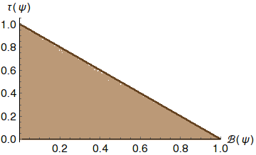
Figure 1: Complementarity between the tangle, $\tau(\psi)$ and the maximum Bell inequality violation, $\mathcal{B}_{\max}(\psi)$ for $10^{6}$ number of Haar uniformly generated random three qubit pure states. The MBV states lies at the boundary. Both axes are dimensionless.

From Theorem 1. and 2., for a three qubit pure state $\ket{\psi}$ either from the $GHZ^{R}$ or the $W$ class, we have $\mathcal{B}_{\max}(\psi)<\mathcal{B}_{\max}(\psi_{m})$ when $\tau(\psi)=\tau(\psi_{m})$. Therefore, for the states in $GHZ^{R}$ and $W$ classes, one has the following complementary relation

$$\tau(\psi)+\mathcal{B}_{\max}(\psi)\leq 1.$$ (21)

In Fig.1, the complementary relation between the tangle and the bipartite Bell inequality violation has been studied for Haar uniformaly generated random three qubit pure states. The numerical evidence suggests that the complementary relation holds in general for all the three qubit pure states. From numerical evidences, we claim that:

For an arbitrary three qubit pure state $\ket{\psi}$, the tangle $\tau(\psi)$, and the maximal bipartite Bell inequality violation $\mathcal{B}_{\max}(\psi)$, follow the complementary relation given in Eq. 21.

Extension to mixed states: In what follows, we will prove that if the complementary relation between the tangle and the maximum bipartite Bell inequality violation holds for all three qubit pure states, then it also holds for three qubit mixed states. We will use the convexity property of the tangle and maximum bipartite Bell inequality violation by the reduced two qubit states respectively, of an arbitrary three qubit mixed states.

Proof.

The tangle of mixed three qubit states has been defined by convex roof construction tangle-mixed , i.e., the tangle of a mixed three qubit quantum state $\rho$ is given as

$$\tau(\rho)=\min_{\{p_{i},|\psi_{i}\rangle\}}\sum_{i}p_{i}\tau(\psi_{i}),$$ (22)

where the minimization is over the all pure state decomposition of $\rho$, such that $\rho=\sum_{i}p_{i}\outerproduct{\psi_{i}}{\psi_{i}}$, where $p_{i}\geq 0$ and $\sum_{i}p_{i}=1.$ The convexity property of the tangle of mixed states follows from the definition itself. Now, we will prove the convexity property of the maximum bipartite Bell inequality violation $\mathcal{B}_{\max}(\rho)$ for three qubit mixed states. The maximum Bell-CHSH value horodecki-mrho for the reduced two qubit system $\rho_{AB}=\Tr_{C}[\rho_{ABC}]$ of a three qubit mixed state $\rho_{ABC}$ is given by

$$\mathcal{S}(\rho_{AB} )=\left|\Tr[(O_{AB}^{m}\otimes\mathbb{I}_{C})\rho_{ABC}]\right|$$

$$= \left|\sum_{i}p_{i}\left(\Tr[\left(O_{AB}^{m}\otimes\mathbb{I}_{C}\right)|\psi_{ABC}^{i}\rangle\langle\psi_{ABC}^{i}|]\right)\right|\,.$$ (23)

Here, $O_{AB}^{m}$ is the optimal Bell-CHSH operator horodecki-mrho for $\rho_{AB}$, $\mathbb{I}_{C}$ is the identity operator on the Hilbert space of $C$, and $\rho_{ABC}=\sum_{i}p_{i}|\psi_{ABC}^{i}\rangle\langle\psi_{ABC}^{i}|$ is an arbitrary pure state decomposition of $\rho_{ABC}$. Now using the subadditivity property of absolute value we have

$$\mathcal{S}(\rho_{AB})\leq\sum_{i}p_{i} \left|\Tr[\left(O_{AB}^{m}\otimes\mathbb{I}_{C}\right)|\psi_{ABC}^{i}\rangle\langle\psi_{ABC}^{i}|]\right|$$

$$= \sum_{i}p_{i}\left|\Tr[O_{AB}^{m}\rho_{AB}^{i}]\right|,$$ (24)

where $\rho_{AB}^{i}=\Tr_{C}[|\psi_{ABC}^{i}\rangle\langle\psi_{ABC}^{i}|]$. In the RHS of the above inequality, $O_{AB}^{m}$ is an non-optimal Bell-CHSH operator for the states $\rho_{AB}^{i}$’s. If it is replaced by $O_{AB}^{i,m}$ that is optimal for $\rho_{AB}^{i}$ i.e., gives the maximum Bell-CHSH value, for $\rho_{AB}^{i}$ for all $i$, then we have

$$\mathcal{S}(\rho_{AB})\leq\sum_{i}p_{i}\left|\Tr[O_{AB}^{i,m}\rho_{AB}^{i}]\right|\,,$$

$$\mathcal{S}\left(\sum_{i}p_{i}\rho_{AB}^{i}\right)\leq\sum_{i}p_{i}\mathcal{S}(\rho_{AB}^{i}).$$ (25)

Similar relations can be shown for the other two subsystems $\rho_{AC}$ and $\rho_{BC}$ as well. Following Eq. (7), the Ineq. (IV.1) can be written as

$$\sqrt{M\left(\sum_{i}p_{i}\rho_{AB}^{i}\right)}\leq\sum_{i}p_{i}\left(\sqrt{M(\rho_{AB}^{i})}\right)\,.$$ (26)

Note that $M(\rho)$ for a two qubit system $\rho$ is defined as in Eq. (7). It is necessary to mention that Eq. (26) is derived for a two qubit system $\rho_{AB}$ which is a convex combination of two qubit states $\rho_{AB}^{i}$’s, where $\rho_{AB}^{i}=\Tr_{C}[|\psi_{ABC}^{i}\rangle\langle\psi_{ABC}^{i}|]$. Therefore, $\rho_{AB}^{i}$’s are rank two states as $|\psi_{ABC}^{i}\rangle$’s are three qubit pure states. However, note that Eq. (26) holds true for any convex combination $\rho_{AB}=\sum_{j}q_{j}\rho_{AB}^{j}$ ($q_{j}\geq 0$, $\sum_{j}q_{j}=1$), of an arbitrary two qubit state $\rho_{AB}$ as we have only used linearity property of trace and sub-additivity property of absolute value in deriving the Eq. (26). Therefore, Eq. (26) implies convexity of the function $\sqrt{M(\rho)}$. As square of a convex non-negative function is still convex conv-analysis , it follows that

$$M\left(\sum_{i}p_{i}\rho_{AB}^{i}\right)\leq\sum_{i}p_{i}\left[M(\rho_{AB}^{i})\right]\,.$$ (27)

Subtracting 1 from both sides we get

$$M\left(\sum_{i}p_{i}\rho_{AB}^{i}\right)-1\leq\sum_{i}p_{i}[M(\rho_{AB}^{i})-1]\,.$$ (28)

Hence, it follows that

$$\max\{0,M(\rho_{AB})-1\}\leq \max\{0,\sum_{i}p_{i}[M(\rho_{AB}^{i})-1]\}$$

$$\leq \sum_{i}p_{i}\max\{0,[M(\rho_{AB}^{i})-1]\}$$

$$\mathcal{B}(\rho_{AB})\leq \sum_{i}p_{i}\mathcal{B}(\rho_{AB}^{i})\,.$$ (29)

Similarly,

$$\mathcal{B}(\rho_{BC})\leq \sum_{i}p_{i}\mathcal{B}(\rho_{BC}^{i}),$$ (30)

$$\mathcal{B}(\rho_{AC})\leq \sum_{i}p_{i}\mathcal{B}(\rho_{AC}^{i}).$$ (31)

Now, the maximum bipartite Bell Inequality violation, $\mathcal{B}_{\max}(\rho_{ABC})=\max\{\mathcal{B}_{AB}(\rho_{ABC}),\mathcal{B}_{AC}(\rho_{ABC}),$ $\mathcal{B}_{BC}(\rho_{ABC})\}$. Without loss of generality say $\mathcal{B}_{\max}(\rho_{ABC})=\mathcal{B}(\rho_{AB})$. Again,

$$\mathcal{B}(\rho_{AB})\leq \sum_{i}p_{i}\mathcal{B}(\rho_{AB}^{i})$$

$$\leq \sum_{i}p_{i}[\max\{\mathcal{B}(\rho_{AB}^{i}),\mathcal{B}(\rho_{BC}^{i}),\mathcal{B}(\rho_{AC}^{i})\}]$$

$$\leq \sum_{i}p_{i}[\mathcal{B}_{\max}(|\psi_{ABC}^{i}\rangle)].$$ (32)

Therefore,

$$\mathcal{B}_{\max}(\rho_{ABC})\leq\sum_{i}p_{i}[\mathcal{B}_{\max}(|\psi_{ABC}^{i}\rangle)].$$ (33)

Hence, the maximum bipartite Bell inequality violation of a three qubit mixed state is convex.

As the tangle and the maximum bipartite Bell inequality violation of a three qubit mixed state both are convex it implies that the complementary relation in Eq. (21) holds for all three qubit mixed states if it holds for all three qubit pure states. ∎

Therefore, from the support of numerical study for entire $GHZ$ class states, we claim in the following that the complementary relation holds for all three qubit states, not necessarily pure.

Claim 1.

For an arbitrary three-qubit state $\rho$, the tangle $\tau(\rho)$ and the maximum bipartite Bell Inequality violation $\mathcal{B}_{\max}(\rho)$ follows the following complementary relation

$$\tau(\rho)+\mathcal{B}_{\max}(\rho)\leq 1.$$ (34)

IV.2 GGM versus Maximum Bell Inequality Violation

Let us now derive the complementarity between the GGM and the bipartite Bell inequality violation for the $GHZ^{R}$ and $W$ class states.

Lemma 1.

If for a three qubit pure state $\ket{\psi}_{GHZ^{R}}$, the GGM is obtained from, say the $A:BC$ bipartite split, then the only reduced bipartite system of $\ket{\psi}_{GHZ^{R}}$ that can violate the Bell inequality is $\rho_{BC}$.

Proof.

The GGM of the state $\ket{\psi}_{GHZ^{R}}$, is given as $\mathcal{G}(\psi_{GHZ^{R}})=1-\max\{g_{A},g_{B},g_{C}\}$, where $g_{i}$ is the maximum eigenvalue of the reduced state $\rho_{i}$ of $\ket{\psi}_{GHZ^{R}}$, with $i\in\{A,B,C\}$. These maximum eigenvalues, $g_{i}$’s, are given by (see Appendix B),

$$g_{A}=\frac{1}{2}\left(1+\sqrt{1+\frac{s_{\alpha}^{2}(c_{\beta}^{2}c_{\gamma}^{2}-1)s_{2\delta}^{2}}{(1+\mathcal{X})^{2}}}\right),$$ (35)

$$g_{B}=\frac{1}{2}\left(1+\sqrt{1+\frac{s_{\beta}^{2}(c_{\alpha}^{2}c_{\gamma}^{2}-1)s_{2\delta}^{2}}{(1+\mathcal{X})^{2}}}\right),$$ (36)

$$g_{C}=\frac{1}{2}\left(1+\sqrt{1+\frac{s_{\gamma}^{2}(c_{\alpha}^{2}c_{\beta}^{2}-1)s_{2\delta}^{2}}{(1+\mathcal{X})^{2}}}\right),$$ (37)

where, $\mathcal{X}=c_{\alpha}c_{\beta}c_{\gamma}s_{2\delta}$. Let us suppose, without loss of generality, that the GGM is obtained from the bipartite split $A:BC$. Consequently, $\max\{g_{A},g_{B},g_{C}\}=g_{A}$ and $\mathcal{G}(\psi_{GHZ^{R}})=1-g_{A}$.

Now, if $g_{A}>g_{B}$ we obtain the following condition

$$s_{\alpha}^{2}\left(c_{\beta}^{2}c_{\gamma}^{2}-1\right) \geq s_{\beta}^{2}\left(c_{\alpha}^{2}c_{\gamma}^{2}-1\right)$$

$$\Rightarrow\left(c^{2}_{\alpha}-c^{2}_{\beta}\right)s^{2}_{\gamma} \geq 0,$$ (38)

and similarly $g_{A}>g_{C}$ implies

$$\left(c^{2}_{\alpha}-c^{2}_{\gamma}\right)s^{2}_{\beta}\geq 0.$$ (39)

The Bell-CHSH values $M(\rho_{BC})$, $M(\rho_{AC})$ and $M(\rho_{AB})$ for the reduced states $\rho_{BC}$, $\rho_{AC}$ and $\rho_{AB}$ of $\ket{\psi}_{GHZ^{R}}$ (see Appendix C), are given as

$$M(\rho_{BC})=1+\frac{(c_{\alpha}^{2}-c_{\beta}^{2}-c_{\gamma}^{2}+2c_{\beta}^{2}c_{\gamma}^{2})s^{2}_{2\delta}-\mathcal{X}^{2}}{(1+\mathcal{X})^{2}},$$ (40)

$$M(\rho_{AC})=1+\frac{(c_{\beta}^{2}-c_{\alpha}^{2}-c_{\gamma}^{2}+2c_{\alpha}^{2}c_{\gamma}^{2})s^{2}_{2\delta}-\mathcal{X}^{2}}{(1+\mathcal{X})^{2}},$$ (41)

$$M(\rho_{AB})=1+\frac{(c_{\gamma}^{2}-c_{\alpha}^{2}-c_{\beta}^{2}+2c_{\alpha}^{2}c_{\beta}^{2})s^{2}_{2\delta}-\mathcal{X}^{2}}{(1+\mathcal{X})^{2}}.$$ (42)

Now using Eq.(38), we obtain

$$M(\rho_{BC})-M(\rho_{AC})=\frac{2\left(c^{2}_{\alpha}-c^{2}_{\beta}\right)s_{\gamma}^{2}s_{2\delta}^{2}}{(1+\mathcal{X})^{2}}\geq 0.$$ (43)

Similarly, Eq.(39) implies

$$M(\rho_{BC})-M(\rho_{AC})=\frac{2\left(c^{2}_{\alpha}-c^{2}_{\gamma}\right)s_{\beta}^{2}s_{2\delta}^{2}}{(1+\mathcal{X})^{2}}\geq 0.$$ (44)

It follows from the no-go theorem for the Bell Inequality violation that if $\rho_{BC}$ violates the Bell-CHSH inequality, then $M(\rho_{BC})>1$, $M(\rho_{AC})\leq 1$ and $M(\rho_{AB})\leq 1$. Hence, from Eq.(43) and Eq.(44), we get $\mathcal{B}(\rho_{BC})>0$ and $\mathcal{B}(\rho_{AC})=\mathcal{B}(\rho_{AB})=0$.

Note that cyclic permutations of the variables $\alpha$, $\beta$ and $\gamma$ enables one to obtain, say $g_{B}$ and $g_{C}$ from $g_{A}$. Therefore, a similar proof holds for the cases when the GGM is obtained from the other two bipartite splits. This completes the proof of the lemma. ∎

While we have proved Lemma 1. for $GHZ^{R}$ class, a numerical check for $10^{6}$ Haar uniformly generated random $GHZ$ class states indicates that this lemma holds for all the $GHZ$ class states.

Theorem 3.

If $\ket{\psi}_{GHZ^{R}}$ and $\ket{\psi}_{m}$ be two three qubit pure states such that the corresponding GGM, $\mathcal{G}(\psi_{GHZ^{R}})$ and $\mathcal{G}(\psi_{m})$ are equal then the maximal bipartite Bell inequality violations for the two states necessarily follow

$$\mathcal{B}_{\max}(\psi_{m})\geq\mathcal{B}_{\max}(\psi_{GHZ^{R}}).$$ (45)

Proof.

The GGM (Appendix B) and the maximum Bell inequality violation of the MBV state $\ket{\psi}_{m}$ (Appendix C), are given as

$$\mathcal{G}(\psi_{m})=\frac{1}{2}-\frac{m}{1+m^{2}},$$ (46)

$$\mathcal{B}_{\max}(\psi_{m})=\frac{4m^{2}}{(1+m^{2})^{2}},$$ (47)

$$\mathcal{B}_{\max}(\psi_{\mathit{m}})=4\left(\frac{1}{2}-\mathcal{G}(\psi_{\mathit{m}})\right)^{2}.$$ (48)

Let us assume that for $\ket{\psi}_{GHZ^{R}}$, $\max\{g_{A},g_{B},g_{C}\}=g_{A}$, then the GGM is obtained from $A:BC$ bipartite split and

$$\mathcal{G}(\psi_{m})=\mathcal{G}(\psi_{GHZ^{R}})=1-g_{A}\\ =\frac{1}{2}\left(1-\sqrt{1+\frac{s_{\alpha}^{2}(c_{\beta}^{2}c_{\gamma}^{2}-1)s_{2\delta}^{2}}{(1+\mathcal{X})^{2}}}\right).$$ (49)

Then from Eq.(48), we have

$$\mathcal{B}_{\max}(\psi_{\mathit{m}})_{A:BC}=1+\frac{(c_{\alpha}^{2}+c_{\beta}^{2}c_{\gamma}^{2}-1)s_{2\delta}^{2}-\mathcal{X}^{2}}{(1+\mathcal{X})^{2}},$$ (50)

where the subscript $A:BC$ indicates that the GGM of $\ket{\psi}_{GHZ^{R}}$ is obtained from the bipartite split $A:BC$. From Lemma 1., it follows that if GGM is obtained from $A:BC$ split, then only $\mathcal{B}(\rho_{BC})$ can be nonzero and thus $\mathcal{B}_{\max}(\psi_{GHZ^{R}})=\mathcal{B}(\rho_{BC})$. Therefore, to prove theorem 3., we only have to show $\mathcal{B}_{\max}(\psi_{m})_{A:BC}\geq\mathcal{B}(\rho_{BC})$.

Now,

$$\begin{split}&\mathcal{B}_{\max}(\psi_{\mathit{m}})_{A:BC}-\mathcal{B}(\rho_{BC})\\ =\ &1+\frac{(c_{\beta}^{2}s_{\gamma}^{2}-s_{\gamma}^{2})s_{2\delta}^{2}}{(1+\mathcal{X})^{2}}=\ 1-\frac{s_{\beta}^{2}s_{\gamma}^{2}s_{2\delta}^{2}}{(1+\mathcal{X})^{2}}\geq 0,\end{split}$$

as $\mathcal{X}\geq 0$.

Similarly, it can be proved that when $\mathcal{G}(\psi_{GHZ^{R}})=1-{g}_{B}$, or $\mathcal{G}(\psi_{GHZ^{R}})=1-{g}_{C}$, we have $\mathcal{B}_{\max}(\psi_{\mathit{m}})_{B:AC}\geq\mathcal{B}(\rho_{AC})$ or $\mathcal{B}_{\max}(\psi_{\mathit{m}})_{C:AB}\geq\mathcal{B}(\rho_{AB})$ respectively.

Hence, $\mathcal{B}_{\max}(\psi_{m})\geq\mathcal{B}_{\max}(\psi_{GHZ^{R}})$, when $\mathcal{G}(\psi_{m})=\mathcal{G}(\psi_{GHZ^{R}})$. ∎

Now we derive the complementary relation between the Bell inequality violation and GGM of the $W$ class states. The $W$ state, $\frac{1}{\sqrt{3}}(\ket{001}+\ket{010}+\ket{100})$, is the representative for the $W$ class which is a set of all states that can be converted to the $W$ state using SLOCC with non-zero probability. The $W$ class states are given by

$$\ket{\psi}_{W}=\left(\sqrt{d}\ket{000}+\sqrt{a}\ket{001}+\sqrt{b}\ket{010}+\sqrt{c}\ket{100}\right),$$ (51)

where $a+b+c+d=1$ is the normalizing condition, and $a,b,c>0$, $d=1-(a+b+c)\geq 0$ DurVidalCirac . To establish the complementary relation let us first prove the following lemma for $W$ class states.

Lemma 2.

If for a three qubit pure state $\ket{\psi}_{W}$, the GGM is obtained from, say $A:BC$ split, then the only reduced bipartite system of $\ket{\psi}_{W}$ that can violate the Bell inequality is $\rho_{BC}$.

Proof.

The maximum eigenvalues corresponding to the reduced systems $\rho_{A}$, $\rho_{B}$ and $\rho_{C}$ for $\ket{\psi}_{W}$ are respectively given by (see Appendix B),

$$w_{A}=\frac{1}{2}\left(1+\sqrt{1-4(a+b)c}\right),$$ (52)

$$w_{B}=\frac{1}{2}\left(1+\sqrt{1-4(a+c)b}\right),$$ (53)

$$w_{C}=\frac{1}{2}\left(1+\sqrt{1-4(b+c)a}\right),$$ (54)

where $w_{X}$ is the maximum eigenvalue of the subsystem $\rho_{X}$ of state $\ket{\psi_{W}}$, with $X\in\{A,B,C\}$. If we assume that the GGM is obtained from the bipartite split $A:BC$, then it implies that $w_{A}>w_{B}$ and $w_{A}>w_{C}$.

From $w_{A}\geq w_{B}$ and $w_{A}\geq w_{C}$ we respectively get

$$a\left(b-c\right) \geq 0,$$ (55)

$$b\left(a-c\right) \geq 0.$$ (56)

For the reduced states $\rho_{BC}$, $\rho_{AC}$ and $\rho_{AB}$ of $\ket{\psi}_{W}$, the Bell-CHSH values $M(\rho_{BC})$, $M(\rho_{AC})$ and $M(\rho_{AB})$ are (see appendix C) respectively given as

$$M(\rho_{BC})=\frac{1}{2}+\frac{12ab-4ac-4bc+\sqrt{V}}{2},$$ (57)

$$M(\rho_{AC})=\frac{1}{2}+\frac{12ac-4ab-4bc+\sqrt{V}}{2},$$ (58)

$$M(\rho_{AB})=\frac{1}{2}+\frac{12bc-4ab-4ac+\sqrt{V}}{2},$$ (59)

where, $V=[(\sqrt{a}+\sqrt{b}-\sqrt{c})^{2}+d][(\sqrt{a}-\sqrt{b}+\sqrt{c})^{2}+d][(-\sqrt{a}+\sqrt{b}+\sqrt{c})^{2}+d][(\sqrt{a}+\sqrt{b}+\sqrt{c})^{2}+d]$.

Then from Eq.(55) and Eq.(56), one can show

$$M(\rho_{BC})-M(\rho_{AC})=8a\left(b-c\right) \geq 0,$$ (60)

$$M(\rho_{BC})-M(\rho_{AB})=8b\left(a-c\right) \geq 0.$$ (61)

The two equations above demonstrate that $M(\rho_{BC})$ is larger among the three. It follows from the no-go theorem for Bell inequality violation, that when $M(\rho_{BC})>1$, then $M(\rho_{AC})\leq 1$ and $M(\rho_{AB})\leq 1$. Therefore, it follows from Eq.(9), that only $\mathcal{B}(\rho_{BC})>0$ and $\mathcal{B}(\rho_{AC})=\mathcal{B}(\rho_{AB})=0$, when $\mathcal{G}(\psi_{W})=1-w_{A}$. Permutation of parameters $a$, $b$ and $c$ gives rise to the cases when the GGM is obtained from the other two bipartite splits, and follow a similar proof. This completes the proof of the lemma. ∎

From the Lemma 1., Lemma 2. and the numerical studies for $GHZ$ class states we conjecture that for all entangled three qubit pure states, if the bipartite split $X:YZ$ gives the GGM, then among the three reduced bipartite states, only $\rho_{YZ}$ can exhibit the Bell inequality violation.

Theorem 4.

If $\ket{\psi}_{W}$ and $\ket{\psi}_{m}$ are two three qubit pure states such that the respective GGM, $\mathcal{G}(\psi_{W})$ and $\mathcal{G}(\psi_{m})$ are equal, then the maximal bipartite Bell inequality violations necessarily follow

$$\mathcal{B}_{\max}(\psi_{m})\geq\mathcal{B}_{\max}(\psi_{W}).$$ (62)

Proof.

Let us first assume, that $\max\{w_{A},w_{B},w_{C}\}=w_{A}$ and hence, $\mathcal{G}(\psi_{W})=1-w_{A}$. Therefore,

$$\mathcal{G}(\psi_{m})=\mathcal{G}(\psi_{W})=1-w_{A}\\ =\frac{1}{2}\left(1-\sqrt{1-4(a+b)c}\right).$$ (63)

Employing Eq.(48), the corresponding maximum Bell inequality violation for $\ket{\psi}_{m}$ is given as

$$\mathcal{B}_{\max}(\psi_{\mathit{m}} )_{A:BC}=1-4(a+b)c,$$ (64)

with the subscript indicating that the bipartite split $A:BC$ gives the GGM for $\ket{\psi}_{W}$.

From Lemma 2., it follows that only $\mathcal{B}(\rho_{BC})\geq 0$, and hence, $\mathcal{B}_{\max}(\psi_{GHZ^{R}})=\mathcal{B}(\rho_{BC})$. Thus, we only need to show that $\mathcal{B}_{\max}(\psi_{m})_{A:BC}>\mathcal{B}(\rho_{BC})$:

Now,

$$\begin{split}\mathcal{B}_{\max}(\psi_{\mathit{m}})_{A:BC}&-\mathcal{B}(\rho_{BC})\\ =\ &\frac{3}{2}-\frac{4ac+4bc+12ab+\sqrt{V}}{2},\\ \end{split}$$

where $V=[(\sqrt{a}+\sqrt{b}-\sqrt{c})^{2}+d][(\sqrt{a}-\sqrt{b}+\sqrt{c})^{2}+d][(-\sqrt{a}+\sqrt{b}+\sqrt{c})^{2}+d][(\sqrt{a}+\sqrt{b}+\sqrt{c})^{2}+d]$.

It can be shown that the minimum of $\mathcal{B}_{\max}(\psi_{\mathit{m}})_{A:BC}-\mathcal{B}(\rho_{BC})$ is zero, and therefore $\mathcal{B}_{\max}(\psi_{\mathit{m}})_{A:BC}\geq\mathcal{B}(\rho_{BC})$. The same can be proved for the cases when the other two bipartite splits give the GGM, following the cyclic order of the parameters $a$, $b$ and $c$.

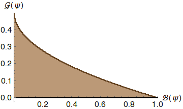
Figure 2: Complementarity between the GGM, $\mathcal{G}(\psi)$ and the maximum Bell inequality violation, $\mathcal{B}_{\max}(\psi)$ for $10^{6}$ number of Haar uniformly generated random three qubit pure states. The MBV states lies at the boundary. Both axes are dimensionless.

∎

From Theorem 3. and 4., for a state $\ket{\psi}$ belonging to either of the $GHZ^{R}$ or $W$ classes, we have that $\mathcal{B}_{\max}(\psi)\leq\mathcal{B}_{\max}(\psi_{m})$, when $\mathcal{G}(\psi)=\mathcal{G}(\psi_{m})$. Hence, for the states in $GHZ^{R}$ and $W$ classes, one can show the following complementary relation

$$4\mathcal{G}(\psi)\big{(}1-\mathcal{G}(\psi)\big{)}+\mathcal{B}_{\max}(\psi)\leq 1.$$ (65)

We study the complementary relation between the GGM and the maximum Bell inequality violation for Haar uniformly generated random genuinely entangled pure three qubit states in Fig.2. Numerical study (appendix D) shows that it holds for all the $GHZ$ class states. Therefore, we propose that the following complementary relation holds for all three qubit pure states.

Claim 2.

For any three qubit pure state $\ket{\psi}$ the GGM, $\mathcal{G}(\psi)$ and the maximal bipartite Bell inequality violation, $\mathcal{B}_{\max}(\psi)$ obey the following complementary relation

$$4\mathcal{G}(\psi)\big{(}1-\mathcal{G}(\psi)\big{)}+\mathcal{B}_{\max}(\psi)\leq 1.$$ (66)

IV.3 Discord Monogamy Score versus Maximum Bell Inequality Violation

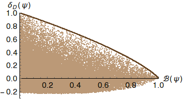
Figure 3: Complementarity between the discord monogamy score, $\delta_{D}(\psi)$ and the maximum Bell inequality violation, $\mathcal{B}_{\max}(\psi)$ for $10^{6}$ number of Haar uniformly generated random three qubit pure states. The MBV states lie at the boundary. Both axes are dimensionless.

Moreover, we study the complementary relation between the discord monogamy score (DMS), and the bipartite Bell inequality violation numerically (see Fig.3). The DMS is not always non-negative as the discord is not monogamous. The MBV states lie at the boundary of the complementary relation in this case too.

V Conclusions

Quantifying nonlocality and finding a relation between nonlocality and quantum correlations is an important yet challenging task in multipartite and higher dimensional quantum systems. In recent past it has been observed that correlation statistics of two body systems can be very fruitful in inferring the multipartite properties of a composite quantum system. In this article we find a single parameter class of states called the MBV class that exhibits the maximum Bell inequality violation for reduced two qubit systems for a fixed amount of genuine tripartite correlation. The measures that we have chosen to quantify genuine tripartite correlation, belong to both the entanglement separability paradigm (the tangle and the GGM) as well as the information theoretic paradigm (DMS). This result in turn establishes a complementary relation between the Bell-CHSH violation by the reduced bipartite systems and the genuine quantum correlations (the tangle) in all three qubit states, with the MBV class lying at the boundary of the complementary relation. The complementary relation between the Bell-CHSH violation by the reduced bipartite systems and the genuine quantum correlations also holds for genuine correlation measure the GGM and the DMS in three qubit pure states, with the MBV class lying at the boundary of the complementary relation. The complementary relation suggests that for all the three measures, the Bell inequality violation of the reduced two party system comes at the cost of genuine tripartite correlations present in the whole system.

Appendix A Expressions for tangle

For a three qubit pure state $\ket{\psi}_{ABC}=\sum_{i,j,k=0}^{1}c_{ijk}\ket{ijk}$, the 3-tangle or the residual tangle Coffmankunduwotters is given as

$$\tau_{ABC} =\tau_{A:BC}-\tau_{AB}-\tau_{AC},$$

$$=4\left|s_{1}-2s_{2}+4s_{3}\right|,$$ (67)

where,

$$s_{1} =c_{000}^{2}c_{111}^{2}+c_{001}^{2}c_{110}^{2}+c_{010}^{2}c_{101}^{2}+c_{100}^{2}c_{011}^{2},$$ (68)

$$s_{2} =c_{000}c_{111}\left(c_{011}c_{100}+c_{101}c_{010}+c_{110}c_{001}\right)$$

$$+c_{011}c_{100}\left(c_{101}c_{010}+c_{110}c_{001}\right)$$

$$+c_{101}c_{010}c_{110}c_{001},$$ (69)

$$s_{3} =c_{000}c_{110}c_{101}c_{011}+c_{111}c_{001}c_{010}c_{100}.$$ (70)

A.1 GHZ Class

For $\ket{\psi}_{GHZ}=\sqrt{K}\left(c_{\delta}\ket{000}+s_{\delta}e^{i\phi}\ket{\varphi_{\alpha}}\ket{\varphi_{\beta}}\ket{\varphi_{\delta}}\right)$ (Eq.(12)), $s_{1}$, $s_{2}$ and $s_{3}$ are respectively given as

$$s_{1} =e^{2i\phi}t_{2}\frac{\left(c_{\delta}^{2}+2e^{2i\phi}t_{1}\right)}{(1+\mathcal{X}_{\phi})^{2}},$$ (71)

$$s_{2} =3e^{3i\phi}t_{1}t_{2}\frac{\left(c_{\delta}+2e^{i\phi}t_{1}\right)}{(1+\mathcal{X}_{\phi})^{2}},$$ (72)

$$s_{3} =e^{3i\phi}t_{1}t_{2}\frac{\left(c_{\delta}+2e^{i\phi}t_{1}\right)}{(1+\mathcal{X}_{\phi})^{2}},$$ (73)

where, $t_{1}=c_{\alpha}c_{\beta}c_{\gamma}s_{\delta}$, $t_{2}=s_{\alpha}^{2}s_{\beta}^{2}s_{\gamma}^{2}s_{\delta}^{2}$ and $\mathcal{X}_{\phi}=c_{\alpha}c_{\beta}c_{\gamma}c_{\phi}s_{2\delta}$. Hence, the tangle of $\ket{\psi}_{GHZ}$ is given as

$$\tau_{GHZ}=\frac{s^{2}_{\alpha}s^{2}_{\beta}s^{2}_{\gamma}s^{2}_{2\delta}}{(1+c_{\alpha}c_{\beta}c_{\gamma}c_{\phi}s_{2\delta})^{2}}$$ (74)

A.2 Maximally Bell inequality violating (MBV) class

For the MBV states $\ket{\psi_{\mathit{m}}}=\frac{\ket{000}+\mathit{m}(\ket{010}+\ket{101})+\ket{111}}{\sqrt{2+2\mathit{m}^{2}}}$ (Eq.(11)), $s_{1}$, $s_{2}$ and $s_{3}$ are respectively given by

$$s_{1} =\frac{1+m^{4}}{4(1+m^{2})^{2}},$$ (75)

$$s_{2} =\frac{m^{2}}{4(1+m^{2})^{2}},$$ (76)

$$s_{3} =0,$$ (77)

and the tangle is,

$$\tau_{m}=1-\frac{4m^{2}}{(1+m^{2})^{2}}.$$ (78)

Appendix B Expressions for GGM

The GGM for a three qubit pure state $\ket{\psi}_{ABC}$, is calculated as

$$\mathcal{G}(\psi_{ABC})=1-\max\{\lambda_{A},\lambda_{B},\lambda_{C}\},$$

where $\lambda_{A}$, $\lambda_{B}$ and $\lambda_{C}$ are the largest eigenvalues of the reduced systems $\rho_{A}$, $\rho_{B}$ and $\rho_{C}$ respectively.

B.1 GHZ Class

For $\ket{\psi}_{GHZ}$, the eigenvalues of the reduced systems $\rho_{A}$, $\rho_{B}$ and $\rho_{C}$ are respectively given as follows.
For subsystem $\rho_{A}$,

$$g_{A}^{\pm}=\frac{1}{2}\left(1\pm\sqrt{1+\frac{s_{\alpha}^{2}(c_{\beta}^{2}c_{\gamma}^{2}-1)s_{2\delta}^{2}}{(1+\mathcal{X_{\phi}})^{2}}}\right),$$

For subsystem $\rho_{B}$,

$$g_{B}^{\pm}=\frac{1}{2}\left(1\pm\sqrt{1+\frac{s_{\beta}^{2}(c_{\alpha}^{2}c_{\gamma}^{2}-1)s_{2\delta}^{2}}{(1+\mathcal{X_{\phi}})^{2}}}\right),$$

For subsystem $\rho_{C}$,

$$g_{C}^{\pm}=\frac{1}{2}\left(1\pm\sqrt{1+\frac{s_{\gamma}^{2}(c_{\alpha}^{2}c_{\beta}^{2}-1)s_{2\delta}^{2}}{(1+\mathcal{X_{\phi}})^{2}}}\right).$$

Here $\mathcal{X_{\phi}}=c_{\alpha}c_{\beta}c_{\gamma}c_{\phi}s_{2\delta}$. In each of the subsystem, it is clear that the eigenvalue $g^{+}_{X}$ is largest, and will be relabeled $g_{X}$, where $X\in\{A,B,C\}$.

B.2 W Class

For $\ket{\psi}_{W}=\sqrt{d}\ket{000}+\sqrt{a}\ket{001}+\sqrt{b}\ket{010}+\sqrt{c}\ket{100}$, the eigenvalues of the reduced subsystems are as follows. For subsystem $\rho_{A}$,

$$w_{A}^{\pm}=\frac{1}{2}\left(1\pm\sqrt{1-4(a+b)c}\right),$$

For subsystem $\rho_{B}$,

$$w_{B}^{\pm}=\frac{1}{2}\left(1\pm\sqrt{1-4(a+c)b}\right),$$

For subsystem $\rho_{C}$,

$$w_{C}^{\pm}=\frac{1}{2}\left(1\pm\sqrt{1-4(b+c)a}\right),$$

Again, the eigenvalue $w^{+}_{X}$ in each pair is largest of the two, where $X\in\{A,B,C\}$.

B.3 MBV class

For $\ket{\psi}_{m}$, the eigenvalues for $\rho_{A}$ and $\rho_{C}$ are $\{1/2,1/2\}$, and eigenvalues of $\rho_{B}$ are given by,

$$\lambda_{B}^{\pm}=\frac{1}{2}\pm\frac{m}{1+m^{2}}.$$

Clearly, $\lambda_{B}^{+}$ is the greatest among all the eigenvalues. Hence, the GGM is given by

$$\mathcal{G}(\psi_{m})=1-\lambda_{B}^{+}=\frac{1}{2}-\frac{m}{1+m^{2}}.$$ (79)

Appendix C Expressions for the Bell inequality violation

Here we give the analytical expressions for the Bell inequality violations for $GHZ^{R}$ and $W$ classes of states, calculated as per the method prescribed by Horodecki et al. horodecki-mrho . The Bell inequality violation is quantified as $\mathcal{B}(\rho_{AB})=\max\{0,M(\rho)-1\}$, where $M(\rho_{AB})$ is the sum of the two largest eignevalues of the matrix, $T_{AB}^{T}T_{AB}$. Here, $T_{AB}$ is the correlation matrix such that $(T_{AB})_{ij}=\mbox{Tr}[(\sigma_{i}\otimes\sigma_{j})\rho_{AB}]$. As we are dealing with three qubit pure states, the Bell inequality violation is calculated for each of the three reduced two qubit systems, $\rho_{AB}$, $\rho_{BC}$ and $\rho_{AC}$.

C.1 $GHZ^{R}$ Class

For the state $\ket{\psi}_{GHZ^{R}}$, the eigenvalues of the matrix $T^{T}_{BC}T_{BC}$ are as follows,

$$\lambda_{1} =\frac{c_{\alpha}^{2}s_{\beta}^{2}s_{\gamma}^{2}s_{\delta}^{2}}{(1+\mathcal{X})^{2}},$$ (80)

$$\lambda_{2} =\mathcal{A}_{BC}-\frac{\sqrt{\mathcal{D}}}{2(1+\mathcal{X})^{2}},$$ (81)

$$\lambda_{3} =\mathcal{A}_{BC}+\frac{\sqrt{\mathcal{D}}}{2(1+\mathcal{X})^{2}},$$ (82)

where, $\mathcal{X}=c_{\alpha}c_{\beta}c_{\gamma}c_{2\delta}$, and

$$\mathcal{A}_{BC}=\frac{1}{2}+\frac{(c_{\alpha}^{2}-c_{\beta}^{2}-c_{\gamma}^{2}+2c_{\beta}^{2}c_{\gamma}^{2})s^{2}_{2\delta}-\mathcal{X}^{2}}{2(1+\mathcal{X})^{2}},$$ (83)

$$\begin{split}\mathcal{D}=1+&4\mathcal{X}+s_{2\delta}^{2}\big{[}-s_{2\delta}^{2}\sum c_{\alpha}+(4\mathcal{X}-2c_{2\delta}^{2})\sum c_{\alpha}^{2}\\ &+2(1+c_{2\delta}^{2})\sum c_{\alpha}^{2}c_{\beta}^{2}-8\mathcal{X}+4\mathcal{X}^{2}\big{]},\end{split}$$ (84)

with $\sum c_{\alpha}=(c_{\alpha}+c_{\beta}+c_{\gamma})$, $\sum c_{\alpha}^{2}=(c_{\alpha}^{2}+c_{\beta}^{2}+c_{\gamma}^{2})$ and $\sum c_{\alpha}^{2}c_{\beta}^{2}=(c_{\alpha}^{2}c_{\beta}^{2}+c_{\alpha}^{2}c_{\gamma}^{2}+c_{\beta}^{2}c_{\gamma}^{2})$.

It can be shown that the eigenvalues are in the following order, $\lambda_{1}<\lambda_{2}<\lambda_{3}$. Thus, the Bell-CHSH value, $M(\rho_{BC})=\lambda_{3}+\lambda_{2}=2\mathcal{A}_{BC}$,

$$M(\rho_{BC})=1+\frac{(c_{\alpha}^{2}-c_{\beta}^{2}-c_{\gamma}^{2}+2c_{\beta}^{2}c_{\gamma}^{2})s^{2}_{2\delta}-\mathcal{X}^{2}}{(1+\mathcal{X})^{2}}.$$ (85)

Similarly, for both the subsystems $\rho_{AC}$ and $\rho_{AB}$, the eigenvalues of $T^{T}_{AC}T_{AC}$ and $T^{T}_{AB}T_{AB}$ respectively, follow the ordering $\lambda_{1}<\lambda_{2}<\lambda_{3}$. The corresponding Bell-CHSH values are given as

$$M(\rho_{AC})=1+\frac{(c_{\beta}^{2}-c_{\alpha}^{2}-c_{\gamma}^{2}+2c_{\alpha}^{2}c_{\gamma}^{2})s^{2}_{2\delta}-\mathcal{X}^{2}}{(1+\mathcal{X})^{2}}.$$ (86)

$$M(\rho_{AB})=1+\frac{(c_{\gamma}^{2}-c_{\alpha}^{2}-c_{\beta}^{2}+2c_{\alpha}^{2}c_{\beta}^{2})s^{2}_{2\delta}-\mathcal{X}^{2}}{(1+\mathcal{X})^{2}}.$$ (87)

There is a inherent exchange symmetry in the expressions, where in, if we swap parameters $\alpha$ and $\beta$ in $M(\rho_{BC})$ we obtain $M(\rho_{AC})$. Similarly, swapping $\beta$ and $\gamma$ in $M(\rho_{AC})$ gives $M(\rho_{AB})$. For each subsystem, we define the Bell inequality violation as $\mathcal{B}(\rho_{XY})=\max\{0,M(\rho_{XY})-1\}$.

C.2 W Class

For the state $\ket{\psi}_{W}$, the eigenvalues for the matrix $T_{BC}^{T}T_{BC}$ are given as,

$$\lambda_{1} =4ab,$$ (88)

$$\lambda_{2} =\frac{1}{2}+2(ab-ac-bc)-\frac{\sqrt{V}}{2},$$ (89)

$$\lambda_{3} =\frac{1}{2}+2(ab-ac-bc)+\frac{\sqrt{V}}{2},$$ (90)

where $a+b+c+d=1$, and $V=[(\sqrt{a}+\sqrt{b}-\sqrt{c})^{2}+d][(\sqrt{a}-\sqrt{b}+\sqrt{c})^{2}+d][(-\sqrt{a}+\sqrt{b}+\sqrt{c})^{2}+d][(\sqrt{a}+\sqrt{b}+\sqrt{c})^{2}+d]$.

The eigenvalues follow the ordering, $\lambda_{2}<\lambda_{1}<\lambda_{3}$, implying $M(\rho_{BC})=\lambda_{1}+\lambda_{3}$,

$$M(\rho_{BC})=\frac{1}{2}+\frac{12ab-4ac-4bc+\sqrt{V}}{2}.$$ (91)

Similarly, for the subsystems $\rho_{AC}$ and $\rho_{AB}$, the eigenvalues for $T_{AC}^{T}T_{AC}$ and $T_{AB}^{T}T_{AB}$ follow the same ordering as mentioned earlier and hence, the Bell-CHSH values for both the bipartitions are given by

$$M(\rho_{AC}) =\frac{1}{2}+\frac{-4ab+12ac-4bc+\sqrt{V}}{2},$$ (92)

$$M(\rho_{AB}) =\frac{1}{2}+\frac{-4ab-4ac+12bc+\sqrt{V}}{2}.$$ (93)

Note that, here too an exchange symmetry similar to the $GHZ^{R}$ class of states holds. By swapping $a$ and $b$ in $M(\rho_{AB})$, we get $M(\rho_{AC})$. Then by swapping $b$ and $c$ we obtain $M(\rho_{BC})$ from $M(\rho_{AC})$. The Bell inequality violations for each subsystem are then obtained as, $\mathcal{B}(\rho_{XY})=\max\{0,M(\rho_{XY})-1\}$.

C.3 MBV class

In case of the MBV class state $\ket{\psi}_{m}$, the correlation matrices for $\rho_{BC}$ and $\rho_{AB}$ are equal and hence the expressions for the Bell-CHSH values are equal. Therefore, only $\rho_{AC}$ can exhibit violation of the Bell Inequality. The eigenvalues for $T_{AC}^{T}T_{AC}$ for $\rho_{AC}$ are then,

$$\lambda_{1} =1,$$ (94)

$$\lambda_{2} =\lambda_{3}=\frac{4m^{2}}{(1+m^{2})^{2}}.$$ (95)

This implies that

$$M(\rho_{AC})=1+\frac{4m^{2}}{(1+m^{2})^{2}}.$$ (96)

Therefore,

$$M(\psi_{m})=1+\frac{4m^{2}}{(1+m^{2})^{2}}.$$ (97)

Appendix D Numerical Method

To perform the numerical study we have generated Haar-uniformly distributed random three qubit pure states. As the sets of fully separable, bi-separable and the ${\it W}$ class states have measure zero with respect to the set of ${\it GHZ}$ class states, almost all of the Haar-uniformly generated random pure states belong to the ${\it GHZ}$ class. This has been cross checked by calculating the non vanishing tangle for the states generated in the aforesaid way. Now for each such randomly generated state we have evaluated the maximum bipartite Bell inequality violation and the three correlation measures, namely the tangle, the GGM and the DMS. We have performed our study for $10^{7}$ number of randomly generated states for each measure. However, the plots exhibit the numerical study for $10^{6}$ number of states.

References

• (1) E. Schrödinger, M. Born, Mathematical Proceedings of the Cambridge Philosophical Society 31 555 (1935); E. Schrödinger, P. Dirac, A. M. Mathematical Proceedings of the Cambridge Philosophical Society 32 446 (1936).
• (2) R. Horodecki, P. Horodecki, M. Horodecki, et al., Rev. Mod. Phys. 81, 865 (2009).
• (3) A. Einstein, B. Podolsky, N. Rosen, Phys. Rev. 47 (10): 777–780 (1935).
• (4) J. Bell, Physics 1 3, 195–200, (1964).
• (5) N. Brunner, D. Cavalcanti, S. Pironio et al., Rev. Mod. Phys. 86 419 (2014).
• (6) J.Clauser, M. Horne, A. Shimony, et al., Phys. Rev. Lett. 23 880 (1969);
• (7) D.M. Greenberger. M Horne, A. Shimony et al., Am. J. Phys. 58, 1131 (1990); N.D. Mermin, Phys. Rev. Lett. 65, 1838 (1990); M. Ardehali, Phys. Rev. A 46, 5375 (1992); A.V. Belinskii and D.N. Klyshko, Phys. Usp. 36 653 (1993); A. Peres, Found. Phys. 29, 589, (1999); I. Pitowsky and K. Svozil, Phys. Rev. A 64, 014102 (2001); I. Pitowsky, Quantum Probabilty–Quantum Logic (Springer, Berlin, 1989); R. F. Werner and M. M. Wolf, Phys. Rev. A 64, 032112 (2001); W. Laskowski, T. Paterek, M. Zukowski et al., Phys. Rev. Lett. 93, 200401 (2004); L. Aolita, R. Gallego, A. Cabello et al., Phys. Rev. Lett. 108, 100401 (2012). M. Żukowski and C. Brukner, Phys. Rev. Lett. 88, 210401 (2001);
• (8) G. Svetlichny, Phys. Rev. D 35, 3066 (1987);
• (9) Michael Redhead, Incompleteness, Nonlocality and Realism, ISBN: 9780198242383.
• (10) A.K. Ekert, Phys. Rev. Lett. 67, 661 (1991); J Barrett, L. Hardy and A. Kent, Phys. Rev.Lett. 95 010503 (2005); A. Acin, N. Brunner, N. Gisinet al, Phys. Rev. Lett. 98, 230501 (2007).
• (11) S. Pironio, A. Acin, S. Massar et al., Nature (London) 464, 1021 (2010); R. Colbeck, Ph.D. Thesis, University of Cambridge, 2007; R. Colbeck and A. Kent, J. Phys. A 44, 095305 (2011).
• (12) C. H. Bennett, S. J. Wisener, Phys. Rev. Lett. 69, 2881 (1992).
• (13) R. Nepal, R. Prabhu, A. Sen(De) et al., Phys. Rev. A 87, 032336 (2013).
• (14) C. H. Bennett, G. Brassard, C Crépeau et al., Phys. Rev. Lett. 70, 1895 (1993); R. Horodecki, M. Horodecki, P. Horodecki, Phys. Lett. A 222 (1996) 21.
• (15) S.K. Sazim, I. Chakrabarty Eur. Phys. J. D 67, 174 (2013); D.Deutsch, A.Ekert, R Jozsa et al, Phys. Rev. Lett. 77, 2818 (1996); L. Goldenberg and L. Vaidman, Phys. Rev. Lett. 75 1239 (1995); A Cabello Phys. Rev. A 61 052312 (2000); C. Li, H-S Song and L. Zhou, Journal of Opptics B: Quantum semiclass. opt. 5 155(2003); A. K. Pati, Phys. Rev. A 63, 014320 (2001); S. Adhikari, B. S. Choudhury, Phys. Rev. A 74 032323 (2006); I. Chakrabarty, B.S. Choudhary arXiv:0804:2568; I. Chakrabarty Intl J. Quant. Inf. 7, 559 (2009); S. Adhikari, A.S. Majumdar, N. Nayak, Phys. Rev. A. 77 042301 (2008); I. Ghiu, Phys. Rev. A 67 012323 (2003); S. Adhikari, I Chakrabarty, B.S. Choudhary, J. Phys. A 39 8439 (2006); V. Buzek, V. Vedral, M.B. Plenio et al., Phys. Rev. A 55 3327 (1997); A Orieux, A. D’Arrigo, G Ferranti et al., arXiv:1410.3678; A. D’Arrigo, R. Lo Franco, G. Benenti et al., Ann. Phys. 350 (2014).
• (16) D. Cavalcanti, A Acin, N. Brunner et al., Phys. Rev. A 87, 042104 (2013).
• (17) N. Gisin, Phys. Lett. A 154, 201 (1991);
• (18) R. Horodecki, P. Horodecki, M. Horodecki, Phys. Lett. A, 200, 340 (1995).
• (19) J. Batle, M. Casas, J. Phys. A: Math. Theor. 44 445304 (2011).
• (20) J. Batle, M. Casas, Phys. Rev. A 82, 062101 (2010).
• (21) S. Ghose, N. Sinclair, S. Debnath et al., Phys. Rev. Lett. 102, 250404 (2009); A. Ajoy and P. Rungta, Phys. Rev. A 81, 052334 (2010).
• (22) D. collins, N. Gisin, S. Popescu et al., Phys. Rev. Lett. 88, 170405 (2002); J.L. Cereceda, phys. Rev. A 66, 024102 (2002).
• (23) N. Brunner, J. Sharam, T. Vertesi, Phys.A:Math.Theor. 43, 385303 (2010); M. Wiesniak, M. Nawareg and M. Zukowski, Phys.Rev. A 86, 042339 (2012); J. Tura, R. Augusiak, A. B. Sainz et al., Science 344 1256 (2014).
• (24) G.Tóth, Phys. Rev. A 71, 010301 (2005); J. Korbickz, J.I Cirac, J. Wehr et al., Phys. Rev. Lett. 94 153601 (2005); G. Tóth, C. Knapp, O Günhe et al., Phys. Rev. Lett. 99, 250405 (2007); O.Gittsovich, P.Hyllus, and O. Günhe, Phys. Rev. A 82, 032306 (2010); M. Markiewicz, W. Laskowski, T. Paterek et al., Phys. Rev. A 87, 034301 (2013).
• (25) A. Shimony, Ann. N.Y. Acad. Sci. 755, 675 (1995); H. Barnum and N. Linden, J. Phys. A 34, 6787 (2001); T.-C. Wei and P.M. Goldbart, Phys. Rev. A 68, 042307 (2003).
• (26) Aditi Sen (De) and Ujjwal Sen, Phys. Rev. A 81, 012308 (2010); T. Das, S. Singha Roy, S. Bagchi et al., arXiv: 1509.02085; D. Sadhukhan, S. Singha Roy, A.K. Pal et al., arXiv:1511.03998.
• (27) V. Coffman, J. Kundu and W. K. Wootters, Phys. Rev. A, 61, 052306 (2000).
• (28) L. Henderson and V. Vedral, J. Phys. A 34, 6899 (2001); H. Ollivier and W. H. Zurek, Phys. Rev. Lett. 88, 017901 (2001); A. Misra, A. Biswas, A. K. Pati et al., Phys. Rev. E 91, 052125 (2015).
• (29) R. Prabhu, A.K. Pati, A Sen(De) et al., Phys. Rev. A 85,040102(R) (2012); G. L. Giorgi, ibid. 84, 054301 (2011).
• (30) M. Koashi and A. Winter, Phys. Rev. A 69, 022309 (2004); T. J. Osborne and F. Verstraete, Phys. Rev. Lett. 96, 220503 (2006); G. Adesso, A. Serafini, and F. Illuminati, Phys. Rev. A 73, 032345 (2006); T. Hiroshima, G. Adesso, and F. Illuminati, Phys. Rev. Lett. 98, 050503 (2007); M. Seevinck, Phys. Rev. A 76, 012106 (2007); S. Lee and J. Park, Phys. Rev. A 79, 054309 (2009); A. Kay, D. Kaszlikowski, and R. Ramanathan, Phys. Rev. Lett. 103, 050501 (2009); & references therein; A. Streltsov, G. Adesso, M. Piani et al., Phys. Rev. Lett. 109, 050503 (2012).
• (31) S. Hill and W.K. Wootters, Phys. Rev. Lett. 78, 5022 (1997).
• (32) W. Dür, G. Vidal, J. I. Cirac, Phys. Rev. A 62, 062314 (2000).
• (33) D. Sadhukhan, S. Singha Roy, D. Rakshit et al., New J. Phys. 17 043013 (2015).
• (34) T.R. de Oliveira, A. Saguia and M.S. Sarandy, EPL 100, 60004 (2012).
• (35) A. Osterloh, J. Siewert, and A. Uhlmann, Phys. Rev. A 77, 032310 (2008)
• (36) Convex Analysis by R. T. Rockafellar, Princeton Uni. Press (1997).