GreenInfra: Capacity of Large-Scale Hybrid Networks With Cost-Effective Infrastructure

Abstract

The cost-effective impact and fundamental limits of infrastructure support with rate-limited wired backhaul links (i.e., GreenInfra support), directly connecting base stations (BSs), are analyzed in a large-scale hybrid network of unit node density, where multi-antenna BSs are deployed. We consider a general scenario such that the rate of each BS-to-BS link scales at an arbitrary rate relative to the number of randomly located wireless nodes, $n$. For the operating regimes with respect to the number of BSs and the number of antennas at each BS, we first analyze the minimum rate of each backhaul link, $C_{\textrm{BS}}$, required to guarantee the same throughput scaling as in the infinite-capacity backhaul link case. We then identify the operating regimes in which the required rate $C_{\textrm{BS}}$ scales slower than $n^{\epsilon}$ for an arbitrarily small $\epsilon>0$ (i.e., the regimes where $C_{\textrm{BS}}$ does not need to be infinitely large). We also show the case where our network with GreenInfra is fundamentally in the infrastructure-limited regime, in which the performance is limited by the rate of backhaul links. In addition, we derive a generalized throughput scaling law including the case where the rate of each backhaul link scales slower than $C_{\textrm{BS}}$. To validate the throughput scaling law for finite values of system parameters, numerical evaluation is also shown via computer simulations.

I Introduction

In [1], the sum-rate scaling was originally introduced and characterized in large wireless ad hoc networks. In practice, however, there will be a long latency and insufficient energy with only wireless connectivity in ad hoc networks. Hence, it would be good to deploy infrastructure nodes, or equivalently base stations (BSs), in the network model, i.e., hybrid networks, thereby possibly improving the throughput scaling.

In most network applications, energy efficiency and cost effectiveness are key performance measures for greenness [2, 3, 4, 5, 6, 7] along with the throughput. This is because 1) the operating cost of BSs, driven in part by inefficient diesel power generators, is one of the largest concerns and 2) given the economic and environmental cost, there is a need of environmental grounds to reduce the energy requirement of network architecture. From a telecommunications operator’s point of view, the following two benefits can arise from green communications: reduced energy and network deployment costs, and improved environmental effects. Especially for large-scale hybrid networks with long-distance wired backhaul links connecting all the BSs, the deployment cost of infrastructure is a critical issue for service providers since it not only directly relates to the CapEx (capital expenditures) as well as OpEx (operational expenditures) [8, 9] but also can have significant environmental impacts [10, 11, 12]. Moreover, the increasing number of small cells in the fifth generation (5G) will result in a significant growth in the number of connections between cell sites. First of all, high CapEx/OpEx associated with high backhaul costs may limit the usefulness of such infrastructure-supported protocols in large hybrid networks [13, 14, 15, 16, 17, 18, 19]. It is thus vital to significantly dimension the backhaul bandwidth (or equivalently the backhaul capacity) to reduce the cost of the operators [20].

I-A Main Contributions

In this paper, by taking into account greenness in hybrid networks, we introduce a more general hybrid network with cost-effective infrastructure (named GreenInfra), where the rate of each BS-to-BS link scales at an arbitrary rate relative to the number of nodes, $n$. GreenInfra nodes equipped with a large number of antennas are deployed in the network, and the best among the two BS-supported schemes in [19], i.e., infrastructure-supported single-hop (ISH) and infrastructure-supported multihop (IMH) protocols, is used to characterize an aggregate throughput of the network. More precisely, only infrastructure-supported routing protocols are used for analysis since our main focus is on how the rate of each backhaul link needs to effectively scale. That is, no pure ad hoc routing protocols such as multihop (MH) [1] and hierarchical cooperation [21] are taken into account. Then, we generalize the throughput scaling result achieved by the ISH and IMH protocols with an arbitrary scaling of each backhaul link, which is not definitely straightforward.

Our results present a cost-effective approach for the deployment of backhaul links connecting a great deal of cell sites (i.e., BSs). In order to provide a cost-effective solution to the design of GreenInfra, we first derive the minimum rate of each BS-to-BS link, denoted by $C_{\textrm{BS}}$, required to guarantee the same throughput scaling as in the network using infinite-capacity backhaul links. The required backhaul link rate $C_{\textrm{BS}}$ is shown according to the two-dimensional operating regimes with respect to the number of BSs and the number of antennas at each BS. This backhaul link rate is determined by the multiplication of the number of matched source–destination (S–D) pairs between any different two cells and the BS-to-BS transmission rate for each S–D pair, which is not straightforward since the number of active S–D pairs between two cells and the BS-to-BS transmission rate vary according to the operating regimes. Surprisingly, it turns out that, for some operating regimes, the required backhaul link rate $C_{\textrm{BS}}$ can be indeed sufficiently small, which scales much slower than $n^{\epsilon}$ for an arbitrarily small $\epsilon>0$, and thus does not need to be infinitely large.

Large-scale ad hoc networks are shown to be fundamentally power-limited and/or bandwidth-limited [22]. In addition, we are interested in further identifying the infrastructure-limited regime in which the routing protocol cannot achieve its maximum throughput scaling due to the small backhaul link rate. From the infrastructure-limited regime, one can find the operating regimes, in which the associated throughput scaling can be improved by increasing the backhaul link rate for network design. Finally, we analyze the aggregate throughput scaling for realistic hybrid networks including the case where the rate of each backhaul link scales slower than $C_{\textrm{BS}}$, which is based on the derivation of the transmission rate for each infrastructure-supported routing protocol. To validate the throughput scaling law for finite values of system parameters, we also provide numerical results via comprehensive computer simulations, which are shown to be consistent with our achievability results.

Our results indicate that a judicious rate scaling of each BS-to-BS link under a given operating regime leads to the order optimality of our general hybrid network along with GreenInfra. In other words, we can still achieve the optimal throughput scaling of the network by significantly reducing the backhaul link rate (equivalently, the cost of backhaul links). On the other hand, we note that, in the next generation communications, the wireless backhaul is considered as an alternative to wired backhaul [20]. Our generalized scaling result provides the theoretical limit on the performance of the wireless backhaul whose link rate can be smaller than the minimum required rate.

Our main contribution is fourfold as follows:

• As a cost-effective backhaul solution, we derive the minimum rate of each backhaul link required to achieve the same throughput scaling law as in the infinite-capacity backhaul link case.

• To better understand the fundamental capabilities of our hybrid network with GreenInfra, we explicitly identify the infrastructure-limited regime according to the number of BSs, the number of antennas at each BS, and the rate of each backhaul link.

• To show a more general achievability result, we derive the aggregate throughput scaling with respect to an arbitrary rate scaling of each backhaul link.

• We show the numerical results via computer simulations.

I-B Organization

The rest of this paper is organized as follows. In Section III, system and channel models are described. Routing protocols with infrastructure support are presented in Section IV. In Section V, the minimum required rate of each BS-to-BS link to achieve the capacity scaling with infinite-capacity backhaul is derived. The infrastructure-limited regime is identified in Section VI. The general throughput scaling with an arbitrary rate scaling of each BS-to-BS link is also analyzed in Section VII. In Section VIII, the numerical results are presented. Finally, we summarize our paper with some concluding remarks in Section IX.

I-C Notations

Bold upper and lower case letters denote matrices and vectors, respectively. The superscript $T$ and $\dagger$ denote the transpose and conjugate transpose, respectively, of a matrix (or a vector). The $N\times N$ identity matrix is denoted by $\mathbf{I}_{N}$. The expectation is denoted by $\mathbb{E}[\cdot]$.

II Previous Work

It was shown that, for the dense network having $n$ nodes, randomly distributed in a unit area, the total throughput scales as $\Theta(\sqrt{n/\operatorname{log}n})$ [1]. This throughput scaling is achieved by the MH scheme, where packets of a source are conveyed to the corresponding destination using the nearest-neighbor MH transmission. There have been further studies on MH in the literature [23, 24, 25], while the total throughput scales far less than $\Theta(n)$. In [21], the throughput scaling of the network having unit area was improved to an almost linear scaling, i.e., $\Theta(n^{1-\epsilon})$ for an arbitrarily small $\epsilon>0$, by using a hierarchical cooperation strategy, where packets of a source are delivered to the corresponding destination using a long-range multiple-input multiple-output transmission between clusters recursively. Besides the hierarchical cooperation scheme [21, 26], there have been various research directions to improve the dense network throughput up to a linear scaling by using node mobility [27], interference alignment [28], directional antennas [29], and infrastructure support [13].

To further improve the throughput performance with low latency and low energy, hybrid networks consisting of both wireless ad hoc nodes and infrastructure nodes have been extensively studied in [13, 14, 15, 16, 17, 18, 19, 30] by showing that BSs can be indeed beneficial in improving the network throughput. Moreover, one of the most viable ways to meet growing traffic demands for the high data rate is to use large-scale (massive) multiple antennas at each BS [31, 32]—such large-scale multiple antenna systems can be thought to be easily implemented in very high frequency bands (e.g., millimeter wave bands [33]). Especially, in a hybrid network where each BS is equipped with a large number of antennas, the optimal capacity scaling was characterized in [19]—the achievability result is based on using one of two infrastructure-supported routing protocols, i.e, ISH and IMH protocols, pure MH transmission, and hierarchical cooperation strategy.

It is hardly realistic to assume that BSs are interconnected by infinite-capacity wired links in hybrid networks [13, 14, 15, 16, 17, 18, 19]. Hence, it is fundamentally important to characterize a new hybrid network with rate-limited backhaul links. In [34, 35], finite-capacity backhaul links between BSs were taken into account in studying performance of the multi-cell processing in cooperative cellular systems based on Wyner-type models which simplify practical cellular systems. In [36, 37], the throughput scaling laws were studied for one- and two-dimensional hybrid networks, where the wired link interconnecting BSs is rate-limited. However, the network model under consideration was comparatively simplified, and the form of achievable schemes was limited only to MH routings.

III System and Channel Models

We consider an extended network of unit node density, where $n$ nodes are uniformly and independently distributed on a square of area $n$, except for the area covered by BSs. It is assumed that a source and its destination are paired randomly, so that each node acts as a source and has exactly one corresponding destination node. Assume that the BSs are neither sources nor destinations. As illustrated in Fig. 1, the whole area of the network is divided into $m$ square cells of equal area. At the center of each cell, there is one BS equipped with $l$ antennas. The total number of antennas in the network is assumed to scale at most linearly with $n$, i.e., $ml=O(n)$. This network configuration basically follows that of [19].

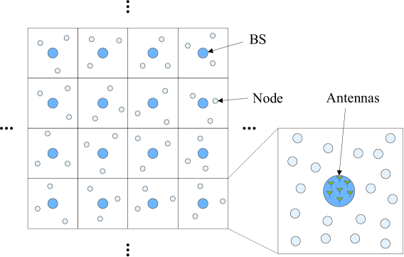
Figure 1: The hybrid network with infrastructure nodes.

For analytical convenience, the parameters $n$, $m$, and $l$ are related according to $n=m^{1/\beta}=l^{1/\gamma}$, where $\beta,\gamma\in[0,1)$ with a constraint $\beta+\gamma\leq 1$. It is assumed that BSs are directly interconnected by wired links. In the previous work [13, 14, 15, 16, 17, 18, 19], it is assumed that the rate of BS-to-BS links is unlimited so that the links are not a bottleneck when packets are delivered from one cell to another. In practice, however, each BS-to-BS link has a finite capacity that may limit the transmission rate of infrastructure-supported routing protocols. In this paper, it is assumed that each BS is connected to each other through an errorless wired link with finite rate $R_{\textrm{BS}}=n^{\eta}$ for $-\infty<\eta<\infty$.

The uplink channel vector between node $i$ and BS $s$ is denoted by

$$\mathbf{h}_{si}^{(u)}=\left[\frac{e^{j\theta_{si,1}^{(u)}}}{r_{si,1}^{\alpha/2}},\frac{e^{j\theta_{si,2}^{(u)}}}{r_{si,2}^{\alpha/2}},\ldots,\frac{e^{j\theta_{si,l}^{(u)}}}{r_{si,l}^{\alpha/2}}\right]^{T},$$ (1)

where $\theta_{si,t}^{(u)}$ represents the random phases uniformly distributed over $[0,2\pi)$ based on a far-field assumption, which is valid if the wavelength is sufficiently small [19]. Here, $r_{si,t}$ denotes the distance between node $i$ and the $t$th antenna of BS $s$, and $\alpha>2$ denotes the path-loss exponent. The downlink channel vector between BS $s$ and node $i$ is similarly denoted by $\mathbf{h}_{is}^{(d)}=\left[\frac{e^{j\theta_{is,1}^{(d)}}}{r_{si,1}^{\alpha/2}},\frac{e^{j\theta_{is,2}^{(d)}}}{r_{si,2}^{\alpha/2}},\ldots,\frac{e^{j\theta_{is,l}^{(d)}}}{r_{si,l}^{\alpha/2}}\right]$. The channel between nodes $i$ and $k$ is given by $h_{ki}=\frac{e^{j\theta_{ki}}}{r_{ki}^{\alpha/2}}$. For the uplink-downlink balance, we assume that each BS satisfies an average transmit power constraint $nP/m$, while each node satisfies an average transmit power constraint $P$. Hence, the total transmit power of all BSs is the same as the total transmit power consumed by all wireless nodes. This assumption on the transmit power is based on the same argument as duality connection between multiple access channel and broadcast channel [38].

It is assumed that the radius of each BS scales as $\epsilon_{0}\sqrt{n/m}$, where $\epsilon_{0}>0$ is an arbitrarily small constant independent of $n$, $m$, and $l$. This radius scaling would ensure enough separation among the antennas provided that per-antenna distance scales (at least) as the average per-node distance $\Omega(1)$ for any parameters $n$, $m$, and $l$. If the radius scaling scales slower than $\Theta(1)$, then per-antenna distance may become vanishingly small, which is undesirable under our infrastructure-supported routing protocols. This antenna configuration basically follows the previous framework established in [19, 39]. Along with the radius scaling of each BS, the antennas of each BS are placed as follows:

1. If $l=w(\sqrt{n/m})$ and $l=O(n/m)$, then $\sqrt{n/m}$ antennas are regularly placed on the BS boundary, i.e., the outermost circle of the BS area, and the remaining antennas are uniformly placed inside the boundary.

2. If $l=O(\sqrt{n/m})$, then $l$ antennas are regularly placed on the BS boundary.

This antenna scaling can be taken into account in large-scale (massive) multiple antenna systems [31, 32].

The per-node throughput of the network $R_{n}$ is assumed to be the average transmission rate measured in bits or packets per unit time. Then, the aggregate throughput of the network is defined as $T_{n}=nR_{n}$. The scaling exponent of the aggregate throughput is defined as

$$e(\alpha,\beta,\gamma,\eta)=\lim_{n\rightarrow\infty}\frac{\operatorname{log}T_{n}(\alpha,\beta,\gamma,\eta)}{\operatorname{log}n}.$$

We will later examine the scaling exponent $e(\alpha,\beta,\gamma,\eta)$ for routing protocols in an operating regime that is identified according to the path-loss exponent, the number of BSs, the number of antennas per BS, and the backhaul link rate.

IV Hybrid Network With Infinite-Capacity Infrastructure

In this section, the overview of routing protocols with infrastructure support and the throughput scaling results under the protocols are provided for readability of remaining sections.

IV-A Routing Protocols With Infrastructure Support

The order-optimal routing protocols supported by BSs having multiple antennas in [19] are described in the following. With the aid of the infrastructure-supported routing protocols, packets of a source are delivered to the corresponding destination of the source using three stages: access routing, BS-to-BS communication, and exit routing. According to the transmission scheme in the access and exit routings, the infrastructure-supported routing protocols are categorized into two different protocols as in the following.

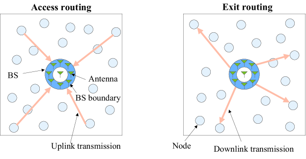
Figure 2: The ISH protocol. Each square represents a cell in the hybrid network.

IV-A1 ISH Protocol

In the ISH protocol, packets of source nodes are transmitted to the BSs via single-hop multiple access, and the BSs transmit the packets to the destination nodes via single-hop broadcast (see Fig. 2, in which two cells are shown). The ISH protocol is described as follows.

• There are $n/m$ nodes with high probability (whp) in each cell [21, Lemma 4.1].

• For the access routing, all source nodes in each cell transmit their packets simultaneously to the home-cell BS via single-hop multiple-access.

• The packets of source nodes are then jointly decoded at each BS, assuming that the signals transmitted from the other cells are treated as noise. The minimum mean-square error (MMSE) estimation with successive interference cancellation (SIC) is performed at each BS. More precisely, the $l\times 1$ receive filter $\mathbf{v}_{i}$ for the signal of the $i$-th node at BS $s$ is given by [38]

  $$\mathbf{v}_{i}=\left(\mathbf{I}_{l}+\sum_{k>i}P\mathbf{h}_{sk}^{(u)}\mathbf{h}_{sk}^{(u)\dagger}\right)^{-1}\mathbf{h}_{si}^{(u)},$$ (2)

  where the signals from nodes $1,\cdots,i-1$ are cancelled and the signals from nodes $i+1,\cdots,n/m$ are treated as noise when the cancelling order is $1,\cdots,n/m$.

• In the next stage, the decoded packets are transmitted to the BS nearest to the corresponding destination of the source via wired BS-to-BS link.

• For the exit routing, the BS in each cell transmits $n/m$ packets received from other cells to the wireless nodes in its cell via single-hop broadcast. The transmit precoding in the downlink is designed by the dual system of the receive filters in the uplink. The $l\times 1$ transmit precoding vector $\mathbf{u}_{i}$ with dirty paper coding (DPC) at BS $s$ is given by [40]

  $$\mathbf{u}_{i}=\left(\mathbf{I}_{l}+\sum_{k>i}p_{k}\mathbf{h}_{ks}^{(d)\dagger}\mathbf{h}_{ks}^{(d)}\right)^{-1}\mathbf{h}_{is}^{(d)\dagger},$$ (3)

  where the power $p_{k}\geq 0$ is allocated to each node such that $\sum_{k}p_{k}\leq\frac{nP}{m}$ for $k=1,\cdots,n/m$.

IV-A2 IMH Protocol

Since the extended network is fundamentally power-limited [21, 22], the ISH protocol may not be effective especially when the node-BS distance is quite long. Thus, we introduce the IMH protocol (see Fig. 3, in which two cells are shown). In the IMH protocol, the packets are transmitted between nodes and BSs using MH routing.

• Each cell is further divided into smaller square cells of area $2\operatorname{log}n$, termed routing cells.

• When $\operatornamewithlimits{min}\{l,\sqrt{n/m}\}$ antennas are regularly placed on the BS boundary, $\operatornamewithlimits{min}\{l,\sqrt{n/m}\}$ MH paths can be used simultaneously.

• For the access routing, the antennas placed only on the home-cell BS boundary can receive the packet transmitted from one of the nodes in the nearest-neighbor routing cell. The MH routing is performed horizontally or vertically by using the adjacent routing cells passing through the line connecting a source to one of the antennas of its BS. The transmission rate scaling per routing path does not depend on the path loss exponent $\alpha$ since the signal-to-interference-and-noise ratio (SINR) seen by any receiver (a BS antenna) is given by $\Omega(1)$ owing to the nearest-neighbor routing.

• The BS-to-BS communication is the same as the ISH protocol.

• For the exit routing, each antenna on the target-cell BS boundary transmits the packets to one of the nodes in the nearest-neighbor routing cell. The packets are transmitted along a line connecting the antenna of its BS to the corresponding destination. The SINR at the receiving node is also given by $\Omega(1)$.

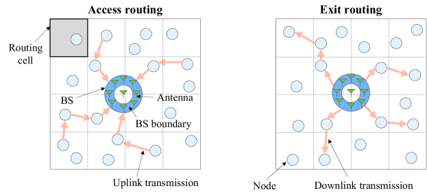
Figure 3: The IMH protocol. Each square represents a cell in the hybrid network. The shaded square in the left figure represents a routing cell.

IV-B The Throughput Scaling With Infinite Backhaul Link Rate

In this subsection, the throughput scaling results of the two routing protocols with infinite backhaul link rate derived in [19] are summarized.

Lemma 1 ([19])

Suppose that the ISH protocol is used in the extended network, where the rate of each BS-to-BS link is unlimited. Then, the aggregate rate scaling is given by

$$T_{n,\textrm{ISH}}=\Omega\left(ml\left(\frac{m}{n}\right)^{\alpha/2-1}\right).$$ (4)

Lemma 2 ([19])

Suppose that the IMH protocol is used in the extended network, where the rate of each backhaul link is unlimited. Then, the aggregate rate scaling is given by

$$T_{n,\textrm{IMH}}=\Omega\left(m\operatornamewithlimits{min}\left\{l,\left(\frac{n}{m}\right)^{1/2-\epsilon}\right\}\right),$$ (5)

where $\epsilon>0$ is an arbitrarily small constant.

Note that unlike the ISH protocol, the aggregate rate scaling of the IMH protocol does not depend on the path loss exponent $\alpha$ since the IMH is designed based on the nearest-neighbor MH. From Lemmas 1 and 2, the aggregate throughput of the network is given by the maximum of these two scaling laws as in the following theorem.

Theorem 1

In the hybrid network of unit node density, where the rate of each backhaul link is unlimited, the aggregate throughput achieved by both ISH and IMH protocols is given by

$$T_{n} =\operatorname{max}\left\{T_{n,\textrm{ISH}},T_{n,\textrm{IMH}}\right\}$$

$$=\Omega\left(\operatorname{max}\left\{ml\left(\frac{m}{n}\right)^{\alpha/2-1},m\operatornamewithlimits{min}\left\{l,\left(\frac{n}{m}\right)^{1/2-\epsilon}\right\}\right\}\right),$$ (6)

where $\epsilon>0$ is an arbitrarily small constant.

In order to better understand the aggregate throughput in (1), two operating regimes with respect to the scaling parameters $\beta$ and $\gamma$ are identified as in Fig. 4. For each regime, we can determine the best routing scheme between ISH and IMH by comparing their throughput scaling exponents. The best routing scheme and its condition are summarized in TABLE I. The throughput achieved by the ISH protocol gets improved with increasing number of antennas per BS, $l$. Thus, the ISH protocol can be used in Regime B. At the high path-loss attenuation regime, since the network is power-limited, the IMH protocol becomes dominant.

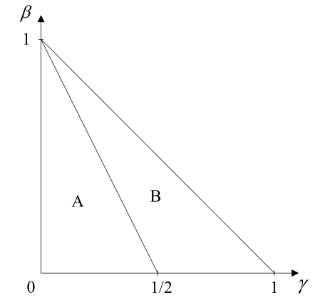
Figure 4: The operating regimes on the throughput scaling with respect to $\beta$ and $\gamma$. Regimes A and B are the set of operating points satisfying $\beta+2\gamma<1$ and $\beta+2\gamma\geq 1$, respectively.

TABLE I: Throughput scaling for an extended network with infinite-capacity infrastructure

Regime	Condition	Scheme	$e(\alpha,\beta,\gamma,\infty)$
A	$\alpha>2$	IMH	$\beta+\gamma$
B	$\alpha<1+\frac{2\gamma}{1-\beta}$	ISH	$1+\gamma-\frac{\alpha(1-\beta)}{2}$
	$\alpha\geq 1+\frac{2\gamma}{1-\beta}$	IMH	$\frac{1+\beta}{2}$

V The Design of Cost-Effective Infrastructure

As the number of BSs, $m$, increases, the number of interconnections between BSs rapidly grows at a rate of $\Theta(m^{2})$, thus resulting in very high CapEx and OpEx in designing high-capacity backhaul links especially in a large-scale hybrid network. Hence, it is crucial to minimize the rate of backhaul links without sacrificing the aggregate throughput of the network.

In this section, we will derive the minimum rate of each backhaul link required to achieve the aggregate throughput scaling in Theorem 1 by analyzing the number of active S–D pairs between two cells according to the two-dimensional operating regimes. The minimum required rate of BS-to-BS links is determined by the multiplication of the number of matched S–D pairs between any different two cells and the transmission rate of the infrastructure-supported protocols for each S-D pair. Packets of these S–D pairs are conveyed through the backhaul link between their associated two cells. The number of matched S–D pairs between any different two cells is first derived in Lemma 3. Using Lemma 3 and the throughput scaling results based on the use of ISH and IMH routing protocols in (4) and (5), respectively, the minimum required rates of backhaul links for the ISH and IMH routing protocols are then derived in Lemmas 4 and 5, respectively. The minimum required rate of each backhaul link to guarantee the maximum throughput capacity scaling in Theorem 1 can be derived by comparing the required rates of backhaul links for the two infrastructure-supported protocols. Let us start from the following lemma, which derives the number of matched S–D pairs between any two different cells.

Lemma 3

Suppose that there are $n^{a}$ simultaneously transmitting source nodes in each cell, where $a$ is a positive constant. A source node in each cell randomly chooses its destination node that is placed in one cell among $n^{b}$ cells, where $b$ is a positive constant. Then, the number of destinations in the $k$th cell whose source nodes are in the $i$th cell, $X_{ki}$, is given by

$$X_{ki}=\left\{\begin{array}[]{ll}O\left(\operatorname{log}n\right)&\textrm{if~{}}a\leq b\\ \Theta\left(n^{a-b}\right)&\textrm{if~{}}a>b\end{array}\right.$$ (9)

whp as $n$ tends to infinity, where $i,k\in\{1,\ldots,m\}$.

Proof:

Refer to Appendix A-A. ∎

The number of S–D pairs between cells depends on the routing type as well as two scaling parameters $\beta$ and $\gamma$. For ease of explanation, we further divide Regimes A and B into smaller sub-regimes as illustrated in Fig. 5.

V-A The Minimum Required Rate for the ISH Protocol

Since the value of $\alpha$ is not manageable but rather affected by the channel characteristics, the minimum required rate of each backhaul link should be computed by taking into account the transmission rate of the ISH protocol maximized over $\alpha$. The required rate of backhaul links for the ISH protocol is derived in the following lemma. In this subsection, we focus on Regime B since the ISH protocol is used only in the regime, as depicted in TABLE I.

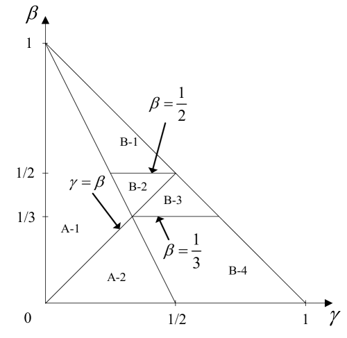
Figure 5: The operating regimes on the required rate of each BS-to-BS link with respect to $\beta$ and $\gamma$.

Lemma 4

Suppose that the ISH protocol is used in Regime B of the network under consideration. Then, the number of destinations in the $k$th cell whose source nodes are in the $i$th cell, $X_{ki}$, is given by

$$X_{ki}=\left\{\begin{array}[]{ll}O\left(\operatorname{log}n\right)&\textrm{for Regime B-1}\\ O\left(n^{1-2\beta}\right)&\textrm{for Regimes B-2, B-3, and B-4,}\\ \end{array}\right.$$ (12)

where $i,k\in\{1,\ldots,m\}$, and $m=n^{\beta}$. The minimum rate of each BS-to-BS link required to achieve the throughput in (4), $C_{\textrm{BS,ISH}}$, is given by

$$C_{\textrm{BS,ISH}}=\left\{\begin{array}[]{ll}\Omega\left(n^{\beta+\gamma-1}\operatorname{log}n\right)&\textrm{for Regime B-1}\\ \Omega\left(n^{\gamma-\beta}\right)&\textrm{for Regimes B-2, B-3, and B-4,}\end{array}\right.$$ (15)

where $l=n^{\gamma}$.

Proof:

Refer to Appendix A-B. ∎

From Lemma 4, it is examined that, as $\beta<\frac{1}{2}$ (i.e., in Regimes B-3, and B-4), the minimum required rate of each backhaul link, $C_{\textrm{BS,ISH}}$, under the ISH protocol grows rapidly with increasing $n$. This is because more data traffic needs to be delivered through each backhaul link in the regime.

V-B The Minimum Required Rate for the IMH Protocol

Since the throughput scaling of the IMH routing protocol has a different form depending on both scaling parameters $\beta$ and $\gamma$, deriving the required rate of each BS-to-BS link for the IMH protocol is not as simple as the ISH routing case. In the following lemma, the required backhaul link rates for the IMH protocol, termed $C_{\textrm{BS,IMH}}$, are characterized with respect to $\beta$ and $\gamma$ by showing three different rates. In this subsection, we focus on whole operating regimes since the IMH protocol can be used in any operating regimes (see TABLE I).

Lemma 5

Suppose that the IMH protocol is used in all the operating regimes of the network under consideration. Then, the number of destinations in the $k$th cell whose source nodes are in the $i$th cell, $X_{ki}$, is given by

$$X_{ki}=\left\{\begin{array}[]{ll}O\left(\operatorname{log}n\right)&\textrm{for Regimes A-1, B-1, B-2, and B-3}\\ O\left(n^{\gamma-\beta}\right)&\textrm{for Regime A-2}\\ O\left(n^{\frac{1-3\beta}{2}-\epsilon}\right)&\textrm{for Regime B-4},\end{array}\right.$$ (19)

where $i,k\in\{1,\ldots,m\}$, $m=n^{\beta}$, $l=n^{\gamma}$, and $\epsilon>0$ is an arbitrarily small constant. The minimum rate of each BS-to-BS link required to achieve the throughput in (5), $C_{\textrm{BS,IMH}}$, is given by

$$C_{\textrm{BS,IMH}}=\left\{\begin{array}[]{ll}\Omega\left(\operatorname{log}n\right)&\textrm{for Regimes A-1, B-1, B-2, and B-3}\\ \Omega\left(n^{\gamma-\beta}\right)&\textrm{for Regime A-2}\\ \Omega\left(n^{\frac{1-3\beta}{2}-\epsilon}\right)&\textrm{for Regime B-4}.\end{array}\right.$$ (23)

Proof:

Refer to Appendix A-C. ∎

From Lemma 5, one can see that the minimum required rate of each backhaul link under the IMH protocol, $C_{\textrm{BS,IMH}}$, is nebligibly small for Regimes A-1, B-1, B-2, and B-3. In other words, in these sub-regimes, the data traffic between BSs is well-distributed to a relatively large number of BSs over the network.

V-C The Minimum Required Rate for the Optimal Infrastructure-Supported Routing Protocols

Based on Lemmas 4 and 5, we are now ready to establish our first main theorem, which characterizes the minimum BS-to-BS link rate guaranteeing the theoretically maximum throughput scaling in Theorem 1 when the best between the ISH and IMH protocols is used according to the operating regimes in our hybrid network with GreenInfra.

Theorem 2

In the hybrid network with GreenInfra, the minimum rate of each BS-to-BS link required to achieve the throughput scaling in Theorem 1, $C_{\textrm{BS}}$, is given by

$$C_{\textrm{BS}}=\left\{\begin{array}[]{ll}\Omega\left(\operatorname{log}n\right)&\textrm{for Regimes A-1, B-1, and B-2}\\ \Omega\left(n^{\gamma-\beta}\right)&\textrm{for Regimes A-2, B-3, and B-4}\end{array}\right.$$ (26)

where $\epsilon>0$ is an arbitrarily small constant. The associated operating regimes with respect to scaling parameters $\beta$ and $\gamma$ are illustrated in Fig. 5.

Proof:

In Regime A, only the IMH protocol is used among the two infrastructure-supported protocols. Thus, $C_{\textrm{BS}}$ is the same as $C_{\textrm{BS,IMH}}$ in these regimes. However, since either the ISH or IMH protocol can be used according to the value of $\alpha$ in Regime B, we should compare the required rates of backhaul links for both protocols using Lemmas 4 and 5. We recall that for the ISH protocol, the required backhaul link rate is maximized over $\alpha$ as in Lemma 4. Then in Regime B-1, $C_{\textrm{BS,ISH}}$ and $C_{\textrm{BS,IMH}}$ are given by $C_{\textrm{BS,ISH}}=\Omega\left((\operatorname{log}n)n^{\beta+\gamma-1}\right)$ and $C_{\textrm{BS,IMH}}=\Omega\left(\operatorname{log}n\right)$, respectively. Since $\beta+\gamma-1\leq 0$, $C_{\textrm{BS,ISH}}$ is smaller than or equal to $C_{\textrm{BS,IMH}}$ in Regime B-1, and thus it follows that $C_{\textrm{BS}}=C_{\textrm{BS,IMH}}=\Omega\left(\operatorname{log}n\right)$ in Regime B-1.

In Regimes B-2 and B-3, $C_{\textrm{BS,ISH}}$ and $C_{\textrm{BS,IMH}}$ are given by $C_{\textrm{BS,ISH}}=\Omega\left(n^{\gamma-\beta}\right)$ and $C_{\textrm{BS,IMH}}=\Omega\left(\operatorname{log}n\right)$, respectively. It thus follows that $C_{\textrm{BS,ISH}}<C_{\textrm{BS,IMH}}$ in Regime B-2 because $\gamma\leq\beta$, while $C_{\textrm{BS,ISH}}>C_{\textrm{BS,IMH}}$ in Regime B-3 because $\gamma>\beta$. Hence, we have

$$C_{\textrm{BS}}=\left\{\begin{array}[]{ll}C_{\textrm{BS,IMH}}=\Omega(\operatorname{log}n)&\textrm{for Regime B-2}\\ C_{\textrm{BS,ISH}}=\Omega\left(n^{\gamma-\beta}\right)&{\textrm{for Regime B-3}}.\end{array}\right.$$ (29)

In Regime B-4, $C_{\textrm{BS,ISH}}$ and $C_{\textrm{BS,IMH}}$ are given by $C_{\textrm{BS,ISH}}=\Omega\left(n^{\gamma-\beta}\right)$ and $C_{\textrm{BS,IMH}}=\Omega\left(n^{\frac{1-3\beta}{2}-\epsilon}\right)$, respectively. The difference of the scaling exponents of $C_{\textrm{BS,ISH}}$ and $C_{\textrm{BS,IMH}}$ is given by $\frac{\beta+2\gamma-1}{2}+\epsilon$. Since $\beta+2\gamma>1$ in Regime B-4, we have $C_{\textrm{BS,ISH}}>C_{\textrm{BS,IMH}}$ and $C_{\textrm{BS}}=C_{\textrm{BS,ISH}}=\Omega\left(n^{\gamma-\beta}\right)$ in Regime B-4. Therefore, the minimum required rate of each BS-to-BS link is finally given by (26), which completes the proof of Theorem 2. ∎

In Regimes A-2, B-3, and B-4, the required rate of each backhaul link is given by $\Omega\left(n^{\gamma-\beta}\right)$. In the regime, the backhaul link rate $C_{\textrm{BS}}$ is increased when the number of antennas per BS, $l$, increases, whereas it is decreased when the number of BSs, $m$, increases.

In Regime B, either the ISH or IMH protocol can be used to achieve the throughput scaling in Theorem 1 according to $\alpha$. Specifically, when $\alpha$ is moderately small, the transmission rate of the ISH protocol is greater than that of the IMH protocol as shown in Lemma 1, while the throughput of the IMH protocol does not depend on $\alpha$. Hence, the required rate $C_{\textrm{BS}}$ of each backhaul link in Regime B should be determined by the maximum of the required rates of backhaul links for the ISH and IMH protocols.

As addressed earlier, the operating regimes A and B are further divided into smaller sub-regimes according to the minimum required rates of backhaul links. More specifically, Regime A is divided into Regimes A-1 and A-2 by the borderline $\gamma=\beta$ since the number of matched S–D pairs is different for the two cases $\gamma\leq\beta$ and $\gamma>\beta$ from Lemma 3. The division of Regime B can be explained in a similar fashion.

Remark 1 (Case of Negligibly Small Backhaul Link Rates)

It is worth noting that, in Regimes A-1, B-1, and B-2, the required rate of each BS-to-BS link is negligibly small, i.e., $C_{\textrm{BS}}=O(n^{\epsilon})$ for an arbitrarily small $\epsilon>0$. This indicates that the backhaul link rate does not need to be infinitely high in these sub-regimes even for a large number of wireless nodes in the network.

VI Identification of the Infrastructure-Limited Regime

The extended network is fundamentally power-limited, i.e., the aggregate throughput is determined by the power transfer between S–D pairs [21, 22]. In our extended network with GreenInfra, the operating regime can also be infrastructure-limited, where the backhaul link rate $R_{\textrm{BS}}$ scales slower than the minimum required rate $C_{\textrm{BS}}$.

In the following, we explicitly identify the infrastructure-limited regime depending on $\eta$ in Figs. 6–7. From Theorem 2, it is seen that, when $\eta\leq 0$, the rate of each backhaul link, $R_{\textrm{BS}}$, scales slower than the minimum required rate $C_{\textrm{BS}}$ in all the operating regimes. Hence, all these regimes are infrastructure-limited if $\eta\leq 0$. It indicates that, unless $\eta>0$, one can achieve only a lower throughput scaling than the ideal throughput scaling in Theorem 1 for any scaling parameters $\beta$ and $\gamma$. If the value of $\eta$ is greater than zero, however, Regimes A-1, B-1, and B-2 becomes not infrastructure-limited since the required rate of each backhaul link in these regimes scales much slower than $n^{\epsilon}$ for an arbitrarily small $\epsilon>0$, as mentioned in Remark 1. When $0<\eta<\frac{1}{2}$, some parts of Regimes A-2, B-3, and B-4 are not infrastructure-limited, and the area of these parts grows as $\eta$ increases. Specifically, if $\eta<\gamma-\beta$, then Regimes A-2, B-3, and B-4 are infrastructure-limited since $C_{\textrm{BS}}=\Omega(n^{\gamma-\beta})$ from Theorem 2, and the associated part is shaded in Fig. 6. If $\frac{1}{2}\leq\eta<1$, then Regimes A-2 and B-3 are no longer infrastructure-limited but a part of Regime B-4 is still infrastructure-limited, which is illustrated in Fig. 7. All operating regimes are not infrastructure-limited if $\eta\geq 1$.

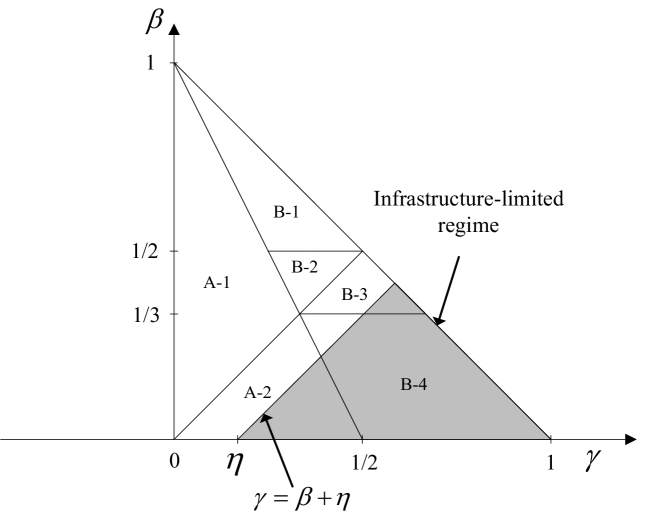
Figure 6: The infrastructure-limited regime with respect to $\beta$ and $\gamma$, where $0<\eta<\frac{1}{2}$.

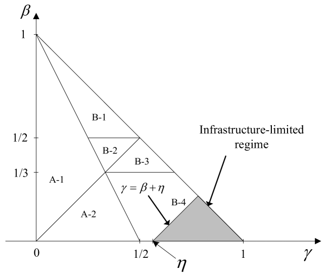
Figure 7: The infrastructure-limited regime with respect to $\beta$ and $\gamma$, where $\frac{1}{2}\leq\eta<1$.

Remark 2

It is worth noting that the backhaul link rate required to guarantee the maximum throughput scaling in Theorem 1 regardless of system parameters $m$ and $l$ is given by $\Omega(\sqrt{n})$ in Regimes A, B-1, B-2, and B-3; and is given by $\Omega(n)$ in Regime B-4, respectively. Hence, it turns out that the minimum rate of each BS-to-BS link, $C_{\textrm{BS}}$, needed regardless of operating regimes (or equivalently, the values of $m$ and $l$) is bounded by $\Omega(n)$.

Remark 3

Using the illustration of the infrastructure-limited regimes, it would be interesting to examine whether or not the backhaul link rate $R_{\textrm{BS}}$ needs to be scaled up when an operating point varies according to scaling parameters $\beta$ and $\gamma$. For example, let us assume that the network is at an operating point $(\beta,\gamma)=(1/2,1/4)$ with $\eta=1/4$. In this case, $R_{\textrm{BS}}$ does not need to be increased until $\gamma$ goes up to $1/2$.

VII Generalized Throughput Scaling With An Arbitrary Backhaul Link Rate

In this section, we shall derive the throughput scaling law for the case where the rate of each BS-to-BS link scales at an arbitrary rate relative to $n$, which generalizes the throughput scaling in Theorem 1. In the following two lemmas, the throughput scaling results for the ISH and IMH protocols operating under infinite-capacity backhaul links shown in Lemmas 1 and 2 are extended to a more general case having an arbitrary backhaul link capacity, $R_{\textrm{BS}}$.

Lemma 6

Suppose that the ISH protocol is used in the hybrid network, where the rate of each BS-to-BS link is limited by $R_{\textrm{BS}}$. Then, the aggregate rate scaling is given by

$$T_{n,\textrm{ISH}}=\Omega\left(\operatornamewithlimits{min}\left\{ml\left(\frac{m}{n}\right)^{\alpha/2-1},m^{2}R_{\textrm{BS}},\frac{n}{\operatorname{log}n}R_{\textrm{BS}}\right\}\right),$$ (30)

where $m=n^{\beta}$.

Proof:

From (A.8) in Lemma 4, for a given transmission rate achieved by the ISH, $T_{n,\textrm{ISH}}$, the minimum required rate of each BS-to-BS link, $C_{\textrm{BS,ISH}}$, is given by

$$C_{\textrm{BS,ISH}}=\left\{\begin{array}[]{ll}\Omega\left(\frac{T_{n,\textrm{ISH}}\operatorname{log}n}{n}\right)&{\rm{if~{}}}\frac{1}{2}\leq\beta<1\\ \Omega\left(\frac{T_{n,\textrm{ISH}}}{m^{2}}\right)&{\rm{if~{}}}0\leq\beta<\frac{1}{2}.\\ \end{array}\right.$$

Hence, substituting a given backhaul link rate $R_{\textrm{BS}}$ into $C_{\textrm{BS,ISH}}$, the transmission rate $T_{n,\textrm{ISH}}$ is given by

$$T_{n,\textrm{ISH}}=\left\{\begin{array}[]{ll}\Omega\left(\operatornamewithlimits{min}\left\{ml\left(\frac{m}{n}\right)^{\alpha/2-1},\frac{n}{\operatorname{log}n}R_{\textrm{BS}}\right\}\right)&{\textrm{if~{}}}\frac{1}{2}\leq\beta<1\\ \Omega\left(\operatornamewithlimits{min}\left\{ml\left(\frac{m}{n}\right)^{\alpha/2-1},m^{2}R_{\textrm{BS}}\right\}\right)&{\textrm{if~{}}}0\leq\beta<\frac{1}{2}.\end{array}\right.$$ (33)

From the fact that $\operatornamewithlimits{min}\left\{\frac{n}{\operatorname{log}n}R_{\textrm{BS}},m^{2}R_{\textrm{BS}}\right\}$ is given by $m^{2}R_{\textrm{BS}}$ and $\frac{n}{\operatorname{log}n}R_{\textrm{BS}}$ as $0\leq\beta<\frac{1}{2}$ and $\frac{1}{2}\leq\beta<1$, respectively, (33) can be simplified to (30). Therefore, $T_{n,\textrm{ISH}}$ is finally given by (30), which completes the proof of Lemma 6. ∎

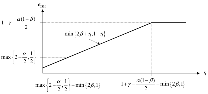
Figure 8: The throughput scaling exponent of the ISH protocol in the network with GreenInfra.

The first term of the right-hand side in (30) corresponds to the rate achieved by the ISH protocol in (4) when the rate of the BS-to-BS link is unlimited. The remaining two terms are the throughput scalings supportable by BSs for an arbitrary $R_{\textrm{BS}}$. The throughput scaling exponent of the ISH protocol is shown in Fig. 8.

Lemma 7

Suppose that the IMH protocol is used in the hybrid network, where the rate of each BS-to-BS link is limited by $R_{\textrm{BS}}$. Then, the aggregate rate scaling is given by

$$T_{n,\textrm{IMH}}=\Omega\left(\operatornamewithlimits{min}\left\{ml,m\left(\frac{n}{m}\right)^{1/2-\epsilon},m^{2}R_{\textrm{BS}},\frac{ml}{\operatorname{log}n}R_{\textrm{BS}},\frac{m}{\operatorname{log}n}\left(\frac{n}{m}\right)^{1/2-\epsilon}R_{\textrm{BS}}\right\}\right),$$ (34)

where $\epsilon>0$ is an arbitrarily small constant.

Proof:

From (A.18) in Lemma 5, for a given transmission rate achieved by the IMH, $T_{n,\textrm{IMH}}$, the minimum required rate of each BS-to-BS link, $C_{\textrm{BS,IMH}}$, is given by

$$C_{\textrm{BS,IMH}}=\left\{\begin{array}[]{ll}\Omega\left(\frac{T_{n,\textrm{IMH}}}{ml}\operatorname{log}n\right)&\textrm{for Regime A-1}\\ \Omega\left(\frac{T_{n,\textrm{IMH}}}{m^{2}}\right)&\textrm{for Regimes A-2 and B-4}\\ \Omega\left(\frac{T_{n,\textrm{IMH}}}{m(n/m)^{1/2-\epsilon}}\operatorname{log}n\right)&\textrm{for Regimes B-1, B-2, and B-3}.\end{array}\right.$$

Hence, substituting a given backhaul link rate $R_{\textrm{BS}}$ into $C_{\textrm{BS,IMH}}$, the transmission rate $T_{n,\textrm{IMH}}$ is given by

$$T_{n,\textrm{IMH}}=\left\{\begin{array}[]{ll}\Omega\left(\operatornamewithlimits{min}\left\{ml,m\left(\frac{n}{m}\right)^{1/2-\epsilon},\frac{ml}{\operatorname{log}n}R_{\textrm{BS}},\frac{m}{\operatorname{log}n}\left(\frac{n}{m}\right)^{1/2-\epsilon}R_{\textrm{BS}}\right\}\right)&\\ {\textrm{for Regimes A-1, B-1, B-2, and B-3}}\\ \Omega\left(\operatornamewithlimits{min}\left\{ml,m\left(\frac{n}{m}\right)^{1/2-\epsilon},m^{2}R_{\textrm{BS}}\right\}\right)\\ {\textrm{for Regimes A-2 and B-4.}}\\ \end{array}\right.$$ (39)

Since $\operatornamewithlimits{min}\left\{\frac{ml}{\operatorname{log}n}R_{\textrm{BS}},\frac{m}{\operatorname{log}n}\left(\frac{n}{m}\right)^{1/2-\epsilon}R_{\textrm{BS}}\right\}$ is given by $\frac{ml}{\operatorname{log}n}R_{\textrm{BS}}$ in Regime A-1 and $\frac{m}{\operatorname{log}n}\left(\frac{n}{m}\right)^{1/2-\epsilon}R_{\textrm{BS}}$ in Regimes B-1, B-2, and B-3, the transmission rate for Regimes A-1, B-1, B-2, and B-3 can be expressed as a single term. Similarly, $T_{n,\textrm{IMH}}$ is finally given by (34), which completes the proof of Lemma 7. ∎

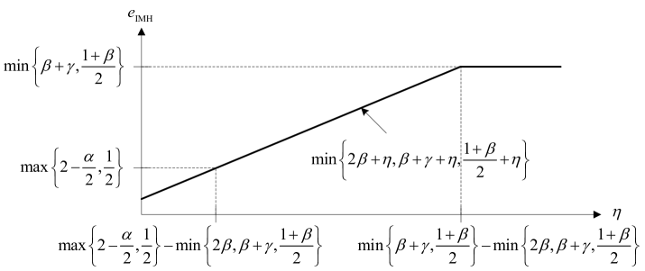
Figure 9: The throughput scaling exponent of the IMH protocol in the network with GreenInfra.

The first two terms of the right-hand side in (34) corresponds to the rate achieved by the IMH protocol in (5) when the rate of backhaul links is not limited. The remaining terms are the throughput that can be supported via backhaul links. The throughput scaling exponent of the IMH protocol is shown in Fig. 9.

Using Lemmas 6 and 7, we finally establish the following theorem, which shows the aggregate throughput along with the rate $R_{\textrm{BS}}$ of each BS-to-BS link.

Theorem 3

In the network with the backhaul link rate $R_{\textrm{BS}}$, the aggregate throughput scales as

$$T_{n}=\operatorname{max}\{T_{n,\textrm{ISH}},T_{n,\textrm{IMH}}\}.$$ (40)

It is easy to show that the transmission rate in (40) is simplified to that in (1) as $R_{\textrm{BS}}\geq C_{\textrm{BS}}$. Furthermore, we remark that the operating regimes on the throughput scaling in (40) with respect to $\beta$ and $\gamma$ depend heavily on the value of $R_{\textrm{BS}}$.

VIII Numerical Evaluation

TABLE II: Simulation environments

Parameter	Value
Average distance between nearest-neighbor nodes	100 m
Transmit power	-10 dBm
Noise spectral density	-174 dBm/Hz
Noise figure	5 dB
Bandwidth	40 MHz

In this section, to validate our achievability result in Section VII in a realistic hybrid network with GreenInfra, we perform computer simulations according to finite values of the system parameters $n$, $m$, $l$, and $R_{\textrm{BS}}$. From (40), the aggregate throughput $T_{n}$ is numerically computed by taking the maximum of $T_{n,\textrm{ISH}}$ and $T_{n,\textrm{IMH}}$ in a certain operating regime. More specifically, the throughput $T_{n,\textrm{ISH}}$ is numerically computed along with the ISH protocol in Section IV-A1, for which the MMSE–SIC postcoder and DPC-based precoder, shown in (2) and (3), respectively, are assumed. The throughput $T_{n,\textrm{IMH}}$ is numerically computed along with the IMH protocol in Section IV-A2. Simulation parameters are summarized in TABLE II. A sufficient number of nodes ($n\geq 256$) are deployed so that a large-scale network is suitably modelled in practice. It is assumed that the average distance between two nearest-neighbor nodes is 100 m (this inter-node distance is sufficient to model an extended network configuration). In our Monte-Carlo simulations, a sufficiently large number of iterations are performed to average out the aggregate throughput for both different node distributions and channels (i.e., phases) under the given system parameters.

The aggregate throughput $T_{n}$ versus the backhaul link rate $R_{\textrm{BS}}$ is first evaluated in Fig. 10, where $n$=1296, $m$=16, $l$=4, and $\alpha\in\{3.5,3.75,4.0\}$. From the figure, the following interesting observations are made under our simulation environments:

• The throughput $T_{n}$ is monotonically increasing with $R_{\textrm{BS}}$ as $R_{\textrm{BS}}<C_{\textrm{BS}}$, where $C_{\textrm{BS}}$ is given by $\{2.0,1.8,1.5\}$ for $\alpha\in\{3.5,3.75,4.0\}$, respectively (see TABLE III).

• For $R_{\textrm{BS}}<C_{\textrm{BS}}$ (i.e., the infrastructure-limited regime), the throughput increases linearly with $R_{\textrm{BS}}$, which is consistent with our analytical prediction (refer to (30)–(40)).

• For $R_{\textrm{BS}}\geq C_{\textrm{BS}}$, the throughput performance is not improved with increasing $R_{\textrm{BS}}$.

• The throughput $T_{n}$ gets significantly reduced as $\alpha$ increases (our scaling results indicate that the transmission rate achieved by the ISH protocol is a non-increasing function of $\alpha$).

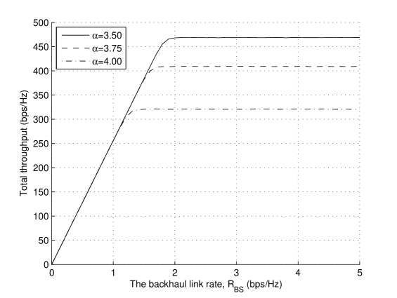
Figure 10: The aggregate throughput $T_{n}$ according to the backhaul link rate, $R_{\textrm{BS}}$, where $n$=1296, $m$=16, and $l$=4.

TABLE III: Evaluation comparison according to the path-loss exponent $\alpha$, where $C_{\textrm{BS}}$ and the maximum $T_{n}$ are shown.

$\alpha$	$C_{\textrm{BS}}$	Maximum value of $T_{n}$
3.5	2.0	468.7
3.75	1.8	409.3
4.0	1.5	322.6

We remark that the most cost-effective way in designing the GreenInfra is to set $R_{\textrm{BS}}=C_{\textrm{BS}}$ while maintaining the maximum throughput we can hope for (i.e., the same throughput as in the infinite-capacity backhaul link case). In addition, the throughput $T_{n}$ versus the number of nodes, $n\in\{256,1296,4096,10000\}$, is evaluated in Fig. 11, where $\alpha$=3.5, $m$=16, $l$=4, and $R_{\textrm{BS}}\in\{0.1,1.0,5.0,10.0\}$. From the figure, the following observations are found:

• It is numerically found that the ISH has a better performance than that of the IMH under the aforementioned simulation environment.

• For this reason, when $R_{\textrm{BS}}<C_{\textrm{BS}}$ (e.g., $R_{\textrm{BS}}=0.1,1.0$ in the figure), the throughput $T_{n}$ is not improved with increasing $n$ since the rate of the ISH is limited to $m^{2}R_{\textrm{BS}}$ (but not to $nR_{\textrm{BS}}$) from (30).

• For $R_{\textrm{BS}}\geq C_{\textrm{BS}}$, the same throughput as in the infinite-capacity backhaul link case is achieved. Thus, the throughput for $R_{\textrm{BS}}=5.0$ is identical to that for $R_{\textrm{BS}}=10.0$, which approaches the maximum we can hope for.

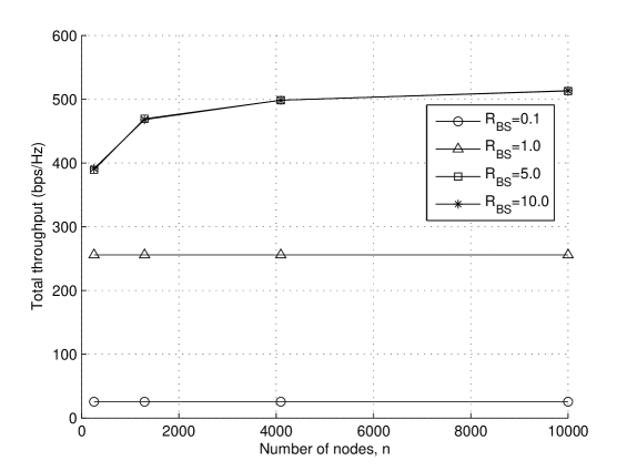
Figure 11: The aggregate throughput $T_{n}$ according to the number of nodes, $n$, where $\alpha$=3.5, $m$=16, and $l$=4.

The throughput $T_{n}$ versus the number of BSs, $m\in\{16,64,144,256\}$, is also evaluated in Fig. 12, where $\alpha$=3.5, $n$=1296, $l$=4, and $R_{\textrm{BS}}\in\{0.1,1.0,5.0,10.0\}$. From the figure, the following observations are found:

• It is numerically found that the ISH protocol is dominant under the simulation environment.

• We first focus on the infrastructure-limited regime (i.e., $R_{\textrm{BS}}<C_{\textrm{BS}}$). In this regime, for small $m$ (e.g., $m=16$), the throughput $T_{n}$ is limited to $m^{2}R_{\textrm{BS}}$ from (30). When $m$ increases, the throughput is now limited to $nR_{\textrm{BS}}$, thereby resulting in no performance improvement for $m\in\{64,144,256\}$.

• Let us turn to the case where $R_{\textrm{BS}}\geq C_{\textrm{BS}}$. The two backhaul link rates $R_{\textrm{BS}}=5.0$ and $R_{\textrm{BS}}=10.0$ lead to the same throughput. It is also seen that the throughput monotonically increases with $m$ due to the fact that its scaling is given by $ml\left(\frac{m}{n}\right)^{\alpha/2-1}$ from (30).

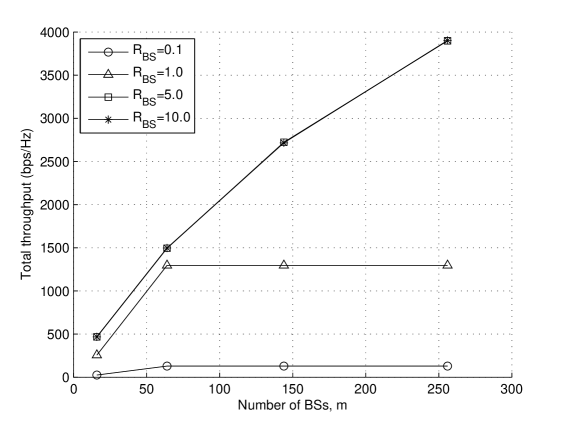
Figure 12: The aggregate throughput $T_{n}$ according to the number of BSs, $m$, where $\alpha$=3.5, $n$=1296, and $l$=4.

Finally, the throughput $T_{n}$ versus the number of antennas per BS, $l\in\{4,8,16,32\}$, is evaluated in Fig. 13, where $\alpha$=3.5, $n$=1296, $m$=16, and $R_{\textrm{BS}}\in\{0.1,1.0,5.0,10.0\}$. From the figure, the following observations are found:

• Similarly, the ISH protocol is dominant under the simulation environment.

• As mentioned before, when $R_{\textrm{BS}}$ is small (e.g., $R_{\textrm{BS}}=0.1,1.0$), the throughput is limited to $m^{2}R_{\textrm{BS}}$ and thus does not depend on $l$.

• We recall Theorem 2, which implies that $C_{\textrm{BS}}$ is given by $n^{\gamma-\beta}$ in Regimes A-2, B-3, and B-4. From Fig. 5, one can see that as $l$ increases, our network approaches one of the three regimes above.

• We consider the case where $R_{\textrm{BS}}=5.0$. In this case, the throughput $T_{n}$ increases with $l$ for small $l$, which means that $R_{\textrm{BS}}\geq C_{\textrm{BS}}$. However, $T_{n}$ is no longer improved beyond a certain value of $l$ ($l=16$ in the figure), which in turn implies that our network is infrastructure-limited.

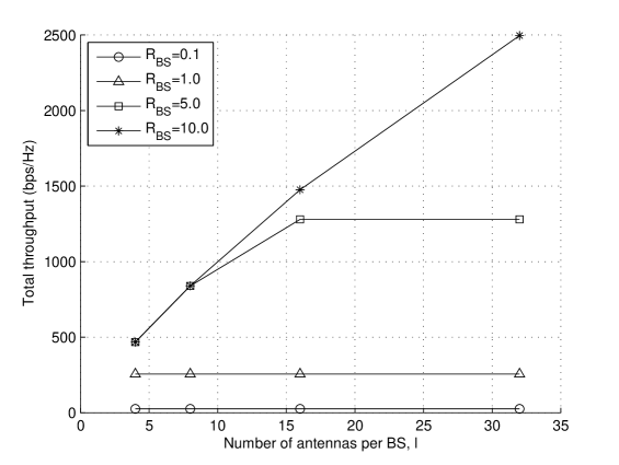
Figure 13: The aggregate throughput $T_{n}$ according to the number of antennas per BS, $l$, where $\alpha$=3.5, $n$=1296, and $m$=16.

IX Concluding Remarks

The large-scale hybrid network with an arbitrary rate scaling of each backhaul link based on the two infrastructure-supported routing protocols, ISH and IMH, was completely characterized. For the two-dimensional operating regimes with respect to the number of BSs, $m$, and the number of antennas at each BS, $l$, the minimum required rate of each BS-to-BS link, $C_{\textrm{BS}}$, was derived to achieve the optimal throughput scaling for a cost-effective backhaul solution. The infrastructure-limited regime was also explicitly identified with respect to the three scaling parameters: $m$, $l$, and the backhaul link rate $R_{\textrm{BS}}$. Furthermore, the generalized throughput scaling was derived including the case for which the backhaul link rate scales slower than the minimum required rate $C_{\textrm{BS}}$. Finally, our scaling results were validated for finite values of $n$, $m$, $l$ and $R_{\textrm{BS}}$ via computer simulations. The numerical results were shown to be consistent with our analysis.

Appendix A Appendix

A-A Proof of Lemma 3

Since each node chooses its destination randomly and independently in a cell among $n^{b}$ cells, the number of destinations in the $k$th cell whose source nodes are in the $i$th cell, $X_{ki}$ does not depend on $k$ and $i$. Hence, we derive $X_{ki}$ for arbitrary $k$ and $i$ as in the following. The probability that the destination node of the $j$th source node in the $i$th cell is in the $k$th cell follows the Bernoulli distribution with probabilities $\Pr\{B_{j}=1\}=1/n^{b}$ and $\Pr\{B_{j}=0\}=1-1/n^{b}$, where $B_{j}$ is the Bernoulli random variable corresponding to the $j$th source node. Note that $B_{j}$’s are independent over $j$ since each node chooses its destination independently. If $a\leq b$, then the probability that the number of destination nodes in the $k$th cell whose source nodes are in the $i$th cell is greater than or equal to $\operatorname{log}n$ is given by

$$\Pr\left\{\sum_{j=1}^{n^{a}}B_{j}\geq\operatorname{log}n\right\}=\Pr\left\{e^{s\sum_{j=1}^{n^{a}}B_{j}}\geq e^{s\operatorname{log}n}\right\}$$

$$\leq\left(\mathbb{E}\left[e^{s\sum_{j=1}^{n^{a}}B_{j}}\right]\right)e^{-s\operatorname{log}n}=\left(\mathbb{E}\left[e^{sB_{1}}\right]\right)^{n^{a}}e^{-s\operatorname{log}n}=\left(e^{s}\frac{1}{n^{b}}+\left(1-\frac{1}{n^{b}}\right)\right)^{n^{a}}e^{-s\operatorname{log}n}$$

$$\leq e^{-n^{a-b}(1-e^{s})-s\operatorname{log}n},$$ (A.1)

where $s$ is a positive real value and $n^{a}$ is the number of source nodes in a cell. Here, the first inequality follows from the Markov inequality, i.e., $\Pr\{X\geq a\}\leq\mathbb{E}[X]/a$ where $X$ is any nonnegative random variable and $a>0$. The last inequality in (A-A) follows from $1+x\leq e^{x}$ for all $x$. Since the right side of the last inequality above tends to zero as $n$ goes to infinity, $X_{ki}$ is given by $O(\operatorname{log}n)$ whp as $n$ goes to infinity if $a\leq b$.

Using [19, Lemma 1], it can be shown that, if $a>b$, then $X_{ki}$ is between $((1-\delta_{0})n^{a-b},(1+\delta_{0})n^{a-b})$, with probability larger than

$$1-n^{b}e^{-\Delta(\delta_{0})n^{a-b}},$$ (A.2)

where $\Delta(\delta_{0})=(1+\delta_{0})\operatorname{ln}(1+\delta_{0})-\delta_{0}$ for $0<\delta_{0}<1$ independent of $n$. The probability in (A.2) tends to one as $n$ increases. Hence, $X_{ki}$ is given by $\Theta(n^{a-b})$ if $a>b$. Therefore, the number of destinations in the $k$th cell whose source nodes are in the $i$th cell is given by (9), which completes the proof of Lemma 3.

A-B Proof of Lemma 4

Since there are $m=n^{\beta}$ cells in the network and $n/m=n^{1-\beta}$ nodes in each cell whp, using Lemma 3, we have

$$X_{ki}=\left\{\begin{array}[]{ll}O\left(\operatorname{log}n\right)&\textrm{if $\beta\geq\frac{1}{2}$}\\ O\left(\frac{n}{m^{2}}\right)&\textrm{if $\beta<\frac{1}{2}$}.\\ \end{array}\right.$$ (A.5)

The operating regime in which $\beta\geq\frac{1}{2}$ is satisfied corresponds to Regime B-1, while the operating regime in which $\beta<\frac{1}{2}$ is satisfied corresponds to Regimes B-2, B-3, and B-4. Hence, $X_{ki}$ is given by (12). Since each source transmits at a rate $T_{n,\textrm{ISH}}/n$ and the number of S–D pairs between two BSs is bounded by (12), the required rate of each BS-to-BS link for the ISH protocol is given by

$$C_{\textrm{BS,ISH}}=\left\{\begin{array}[]{ll}\Omega\left(\frac{T_{n,\textrm{ISH}}\operatorname{log}n}{n}\right)&\textrm{for Regime B-1}\\ \Omega\left(\frac{T_{n,\textrm{ISH}}}{m^{2}}\right)&\textrm{for Regimes B-2, B-3, and B-4}.\end{array}\right.$$ (A.8)

Since the transmission rate achieved by the ISH protocol with infinite backhaul link rate is $T_{n,\textrm{ISH}}=ml\left(\frac{m}{n}\right)^{\alpha/2-1}$ and it is a decreasing function of $\alpha$, the minimum required rate that supports any value of $\alpha$ can be obtained by substituting $\alpha=2$ into (A.8) as follows:

$$C_{\textrm{BS,ISH}}=\left\{\begin{array}[]{ll}\ \Omega\left(\frac{ml\operatorname{log}n}{n}\right)=\Omega\left((\operatorname{log}n)n^{\beta+\gamma-1}\right)&\textrm{for Regime B-1}\\ \Omega\left(\frac{l}{m}\right)=\Omega\left(n^{\gamma-\beta}\right)&\textrm{for Regimes B-2, B-3, and B-4,}\end{array}\right.$$

which completes the proof of Lemma 4.

A-C Proof of Lemma 5

The number of sources in the $i$th cell is denoted by $\mathcal{X}_{i}$. The event that $\mathcal{X}_{i}$ is between $((1-\delta_{0})n/m,(1+\delta_{0})n/m)$ for all $i\in\{1,\ldots,m\}$ is denoted by $A_{\mathcal{X}}$, where $0<\delta_{0}<1$ is a constant independent of $n$. The probability that the destination node of a transmitting source node is in the $k$th cell follows the Bernoulli distribution with probabilities $\Pr\{B_{j}=1\}=1/m$ and $\Pr\{B_{j}=0\}=1-1/m$, where $B_{j}$ is a Bernoulli random variable corresponding to the $j$th transmitting source node and is independent over $j$. The probability that $X_{ki}$ is less than $a$ is given by

$$\Pr\{X_{ki}<a\textrm{ for all }i,k\in\{1,\ldots,m\}\}\geq\Pr\{A_{\mathcal{X}}\}\Pr\{X_{ki}<a\textrm{ for all }i,k|A_{\mathcal{X}}\}$$

$$\geq\Pr\{A_{\mathcal{X}}\}\left(1-m^{2}\Pr\left\{\sum_{j=1}^{\operatornamewithlimits{min}\{l,(n/m)^{1/2-\epsilon}\}}B_{j}\geq a\right\}\right),$$ (A.9)

where $\Pr\{A_{\mathcal{X}}\}\geq 1-n^{\beta}e^{-\Delta(\delta_{0})n^{1-\beta}}$ and $\Delta(\delta_{0})=(1+\delta_{0})\operatorname{log}(1+\delta_{0})-\delta_{0}$. In (A-C), the second inequality holds since the union bound is applied over all $i,k\in\{1,\ldots,m\}$. Note that $\Pr\{A_{\mathcal{X}}\}$ converges to one as $n$ goes to infinity.

In the following, the scaling law of $X_{ki}$ is derived for four cases with respect to $\beta$ and $\gamma$.

1) Regime A-1 $(\beta+2\gamma\leq 1\textrm{~{}and~{}}\gamma\leq\beta)$: Since $\beta+2\gamma\leq 1$, the number of simultaneously transmitting nodes in each cell is $l$. From Lemma 3, we set $a=\operatorname{log}n$ because $\gamma\leq\beta$. Then, we have

$$\Pr\left\{\sum_{j=1}^{l}B_{j}\geq\operatorname{log}n\right\}=\Pr\left\{e^{s\sum_{j=1}^{l}B_{j}}\geq e^{s\operatorname{log}n}\right\}\leq(\mathbb{E}[e^{sB_{1}}])^{l}e^{-s\operatorname{log}n}$$

$$=\left(e^{s}\frac{1}{m}+\left(1-\frac{1}{m}\right)\right)^{l}e^{-s\operatorname{log}n}\leq e^{-(1/m)(1-e^{s})l}e^{-s\operatorname{log}n}=e^{-(1-e^{s})l/m-s\operatorname{log}n},$$ (A.10)

where $s$ is a positive real value. Using (A-C), the probability in (A-C) is given by

$$\Pr\{X_{ki}<\operatorname{log}n\textrm{ for all }i,k\in\{1,\ldots,m\}\} \geq(1-n^{\beta}e^{-\Delta(\delta_{0})n^{1-\beta}})(1-m^{2}e^{-(1-e^{s})l/m-s\operatorname{log}n})$$

$$=(1-n^{\beta}e^{-\Delta(\delta_{0})n^{1-\beta}})(1-e^{2\beta\operatorname{log}n-n^{\gamma-\beta}(1-e^{s})-s\operatorname{log}n}),$$

which converges to one as $n$ goes to infinity by choosing $s=(2+\delta_{0})\beta$, where $m^{2}=e^{2\beta\operatorname{log}n}$.

2) Regime A-2 $(\beta+2\gamma\leq 1\textrm{~{}and~{}}\gamma>\beta)$: Since $\beta+2\gamma\leq 1$, the number of simultaneously transmitting nodes in each cell is $l$. From Lemma 3, we set $a=(1+\delta_{0})\frac{l}{m}$ because $\gamma>\beta$. Then, we have

$$\Pr\left\{\sum_{j=1}^{l}B_{j}\geq(1+\delta_{0})\frac{l}{m}\right\}=\Pr\left\{e^{s\sum_{j=1}^{l}B_{j}}\geq e^{s(1+\delta_{0})l/m}\right\}\leq(\mathbb{E}[e^{sB_{1}}])^{l}e^{-s(1+\delta_{0})l/m}$$

$$=\left(e^{s}\frac{1}{m}+(1-\frac{1}{m})\right)^{l}e^{-s(1+\delta_{0})l/m}\leq e^{-(1/m)(1-e^{s})l}e^{-s(1+\delta_{0})l/m}=e^{-(1-e^{s}+s(1+\delta_{0}))l/m},$$ (A.11)

where $s$ is a positive real value. Using (A-C), the probability in (A-C) is given by

$$\Pr\{X_{ki}<(1+\delta_{0})l/m\}\textrm{ for all }i,k\in\{1,\ldots,m\}\}$$

$$\geq(1-n^{\beta}e^{-\Delta(\delta_{0})n^{1-\beta}})(1-m^{2}e^{-(1-e^{s}+s(1+\delta_{0}))l/m})$$

$$=(1-n^{\beta}e^{-\Delta(\delta_{0})n^{1-\beta}})(1-e^{2\beta\operatorname{log}n-n^{\gamma-\beta}(1-e^{s}+s(1+\delta_{0}))}),$$

which converges to one as $n$ goes to infinity, by choosing $s=\operatorname{log}(1+\delta_{0})$.

3) Regimes B-1, B-2, and B-3 $(\beta+2\gamma>1\textrm{~{}and~{}}\frac{1}{3}\leq\beta<1)$: Since $\beta+2\gamma>1$, the number of simultaneously transmitting nodes in each cell is $(n/m)^{1/2-\epsilon}$. From Lemma 3, we set $a=\operatorname{log}n$ because $\frac{1}{3}\leq\beta<1$. Then, we have

$$\Pr\left\{\sum_{j=1}^{(n/m)^{1/2-\epsilon}}B_{j}\geq\operatorname{log}n\right\} =\Pr\left\{e^{s\sum_{j=1}^{(n/m)^{1/2-\epsilon}}B_{j}}\geq e^{s\operatorname{log}n}\right\}\leq(\mathbb{E}[e^{sB_{1}}])^{(n/m)^{1/2-\epsilon}}e^{-s\operatorname{log}n}$$

$$=\left(e^{s}\frac{1}{m}+\left(1-\frac{1}{m}\right)\right)^{(n/m)^{1/2-\epsilon}}e^{-s\operatorname{log}n}$$

$$\leq e^{-(1/m)(1-e^{s})(n/m)^{1/2-\epsilon}}e^{-s\operatorname{log}n}=e^{-(n/m^{3})^{1/2-\epsilon^{\prime}}(1-e^{s})-s\operatorname{log}n},$$ (A.12)

where $\epsilon^{\prime}>0$ is an arbitrarily small constant and $s$ is a positive real value. Using (A-C), the probability in (A-C) is given by

$$\Pr\{X_{ki}<\operatorname{log}n\textrm{ for all }i,k\in\{1,\ldots,m\}\}$$

$$\geq(1-n^{\beta}e^{-\Delta(\delta_{0})n^{1-\beta}})(1-m^{2}e^{-(n/m^{3})^{1/2-\epsilon^{\prime}}(1-e^{s})-s\operatorname{log}n})$$

$$=(1-n^{\beta}e^{-\Delta(\delta_{0})n^{1-\beta}})(1-e^{2\beta\operatorname{log}n-n^{(1-3\beta)/2-\epsilon^{\prime\prime}}(1-e^{s})-s\operatorname{log}n}),$$

which converges to one as $n$ goes to infinity, by choosing $s=(2+\delta_{0})\beta$.

4) Regime B-4 $(\beta+2\gamma>1\textrm{~{}and~{}}0\leq\beta<\frac{1}{3})$: Since $\beta+2\gamma>1$, the number of simultaneously transmitting nodes in each cell is $(n/m)^{1/2-\epsilon}$. From Lemma 3, we set $a=(1+\delta_{0})^{2}(n/m^{3})^{1/2-\epsilon^{\prime}}$ because $0\leq\beta<\frac{1}{3}$. Then, we have

$$\Pr\left\{\sum_{j=1}^{(n/m)^{1/2-\epsilon}}B_{j}\geq(1+\delta_{0})^{2}\left(\frac{n}{m^{3}}\right)^{1/2-\epsilon^{\prime}}\right\}$$

$$=\Pr\left\{e^{s\sum_{j=1}^{(n/m)^{1/2-\epsilon}}B_{j}}\geq e^{s(1+\delta_{0})^{2}(n/m^{3})^{1/2-\epsilon^{\prime}}}\right\}\leq(\mathbb{E}[e^{sB_{1}}])^{(n/m)^{1/2-\epsilon}}e^{-s(1+\delta_{0})^{2}(n/m^{3})^{1/2-\epsilon^{\prime}}}$$

$$=\left(e^{s}\frac{1}{m}+\left(1-\frac{1}{m}\right)\right)^{(n/m)^{1/2-\epsilon}}e^{-s(1+\delta_{0})^{2}(n/m^{3})^{1/2-\epsilon^{\prime}}}$$

$$\leq e^{-(1/m)(1-e^{s})(n/m)^{1/2-\epsilon}}e^{-s(1+\delta_{0})^{2}(n/m^{3})^{1/2-\epsilon^{\prime}}}=e^{-(n/m^{3})^{1/2-\epsilon^{\prime\prime}}(s(1+\delta_{0})^{2}+1-e^{s})},$$ (A.13)

where $\epsilon^{\prime\prime}>0$ is an arbitrarily small constant and $s$ is a positive real value. Using (A-C), the probability in (A-C) is given by

$$\Pr\{X_{ki}<(1+\delta_{0})^{2}(n/m^{3})^{1/2-\epsilon^{\prime}}\textrm{ for all }i,k\in\{1,\ldots,m\}\}$$

$$\geq(1-n^{\beta}e^{-\Delta(\delta_{0})n^{1-\beta}})(1-m^{2}e^{-(n/m^{3})^{1/2-\epsilon^{\prime}}(s(1+\delta_{0})^{2}+1-e^{s})})$$

$$=(1-n^{\beta}e^{-\Delta(\delta_{0})n^{1-\beta}})(1-e^{2\beta\operatorname{log}n-n^{(1-3\beta)/2-\epsilon^{\prime\prime}}(s(1+\delta_{0})^{2}+1-e^{s})}),$$

which converges to one as $n$ goes to infinity, by choosing $s=\operatorname{log}(1+\delta_{0})$.

From the analysis above, we obtain the number of S–D pairs between two BSs in (19). Since the transmission rate of each source is $T_{n,\textrm{IMH}}/n$ and $\operatornamewithlimits{min}\{l,(n/m)^{1/2-\epsilon}\}$ nodes among $n/m$ source nodes in each cell simultaneously transmit their packets, the rate of each backhaul link between two BSs is given by $\frac{T_{n,\textrm{IMH}}}{n}\frac{n}{m}\frac{1}{\operatornamewithlimits{min}\{l,(n/m)^{1/2-\epsilon}\}}$. Therefore, the required rate is given by

$$C_{\textrm{BS,IMH}}=\left\{\begin{array}[]{ll}\Omega\left(\frac{T_{n,\textrm{IMH}}}{ml}\operatorname{log}n\right)=\Omega(\operatorname{log}n)&\textrm{for Regime A-1}\\ \Omega\left(\frac{T_{n,\textrm{IMH}}}{ml}\frac{l}{m}\right)=\Omega(\frac{l}{m})&\textrm{for Regime A-2}\\ \Omega\left(\frac{T_{n,\textrm{IMH}}}{m(n/m)^{1/2-\epsilon}}\operatorname{log}n\right)=\Omega\left(\operatorname{log}n\right)&\textrm{for Regimes B-1, B-2, and B-3}\\ \Omega\left(\frac{T_{n,\textrm{IMH}}}{m(n/m)^{1/2-\epsilon}}n^{-\epsilon}\sqrt{\frac{n}{m^{3}}}\right)=\Omega\left(n^{-\epsilon}\sqrt{\frac{n}{m^{3}}}\right)&\textrm{for Regime B-4},\end{array}\right.$$ (A.18)

which completes the proof of Lemma 5.

References

- [1] P. Gupta and P. R. Kumar, “The capacity of wireless networks,” IEEE Trans. Inform. Theory, vol. 46, no. 2, pp. 388–404, Mar. 2000.
- [2] Z. Niu, Y. Wu, and Z. Yang, “Cell zooming for cost-efficient green cellular networks,” IEEE Commun. Mag., vol. 48, no. 11, pp. 74–79, Nov. 2010.
- [3] C. Han, T. Harrold, S. Armour, I. Krikidis, S. Videv, P. M. Grant, H. Haas, J. S. Thompson, I. Ku, C.-X. Wang, T. A. Le, M. R. Nakhai, J. Zhang, and L. Hanzo, “Green radio: Radio techniques to enable energy-efficient wireless networks,” IEEE Commun. Mag., vol. 49, no. 6, pp. 46–54, June 2011.
- [4] E. Oh, B. Krishnamachari, X. Liu, and Z. Niu, “Toward dynamic energy-efficient operation of cellular network infrastructure,” IEEE Commun. Mag., vol. 49, no. 6, pp. 56–61, June 2011.
- [5] I. Ashraf, F. Boccardi, and L. Ho, “SLEEP mode techniques for small cell deployments,” IEEE Commun. Mag., vol. 49, no. 8, pp. 72–79, Aug. 2011.
- [6] G. P. Fettweis and E. Zimmermann, “ICT energy consumption – trends and challenges,” in Proc. Int. Symp. Wireless Personal Multimedia Commun. (WPMC), Sendai, Japan, Sept. 2008.
- [7] W.-Y. Shin, H. Yi, and V. Tarokh, “Energy-efficient base-station topologies for green cellular networks,” in Proc. IEEE Int. Consumer Commun. Netw. Conf. (CCNC), Las Vegas, NV, Jan. 2013, pp. 91–96.
- [8] Y. Chen, S. Zhang, and S. Xu, “Characterizing energy efficiency and deployment efficiency relations for green architecture design,” in Proc. IEEE Int. Conf. Communications (ICC), Cape Town, South Africa, May 2010, pp. 1–5.
- [9] Y. Chen, S. Zhang, S. Xu, and G. Ye Li, “Fundamental trade-offs on green wireless networks,” IEEE Commun. Mag., vol. 49, no. 6, pp. 30–37, June 2011.
- [10] A. Fehske, G. Fettweis, J. Malmodin, and G. Biczók, “The global footprint of mobile communications: The ecological and economic perspective,” IEEE Commun. Mag., vol. 49, no. 8, pp. 55–62, Aug. 2011.
- [11] V. Mancuso and S. Alouf, “Reducing costs and pollution in cellular networks,” IEEE Commun. Mag., vol. 49, no. 8, pp. 63–71, Aug. 2011.
- [12] C. Despins, F. Labeau, T. L. Ngoc, R. Labelle, M. Chériet, C. Thibeault, F. Gagnon, A. Leon-Garcia, O. Cherkaoui, B. S. Arnaud, S. Arnaud, J. McNeill, Y. Lemieux, and M. Lemay, “Leverating green communications for carbon emission reductions: Techniques, testbeds, and emerging carbon footprint standards,” IEEE Commun. Mag., vol. 49, no. 8, pp. 101–109, Aug. 2011.
- [13] A. Zemlianov and G. de Veciana, “Capacity of ad hoc wireless networks with infrastructure support,” IEEE J. Select. Areas Commun., vol. 23, no. 3, pp. 657–667, Mar. 2005.
- [14] O. Dousse, P. Thiran, and M. Hasler, “Connectivity in ad-hoc and hybrid networks,” in Proc. IEEE INFOCOM, New York, NY, June 2002, pp. 1079–1088.
- [15] S. R. Kulkarni and P. Viswanath, “Throughput scaling for heterogeneous networks,” in Proc. IEEE Int. Symp. Inf. Theory (ISIT), Yokohama, Japan, Jun./Jul. 2003, p. 452.
- [16] U. C. Kozat and L. Tassiulas, “Throughput capacity of random ad hoc networks with infrastructure support,” in Proc. ACM MobiCom, San Diego, CA, Sept. 2003, pp. 55–65.
- [17] B. Liu, Z. Liu, and D. Towsley, “On the capacity of hybrid wireless networks,” in Proc. IEEE INFOCOM, San Francisco, CA, Mar./Apr. 2003, pp. 1543–1552.
- [18] B. Liu, P. Thiran, and D. Towsley, “Capacity of a wireless ad hoc network with infrastructure,” in Proc. ACM MobiHoc, Montréal, Canada, Sept. 2007, pp. 239–246.
- [19] W.-Y. Shin, S.-W. Jeon, N. Devroye, M. H. Vu, S.-Y. Chung, Y. H. Lee, and V. Tarokh, “Improved capacity scaling in wireless networks with infrastructure,” IEEE Trans. Inform. Theory, vol. 57, no. 8, pp. 5088–5102, Aug. 2011.
- [20] O. Tipmongkolsilp, S. Zaghloul, and A. Jukan, “The evolution of cellular backhaul technologies: Current issues and future trends,” IEEE Commun. Surveys & Tutorials, vol. 13, no. 1, pp. 97–113, First 2011.
- [21] A. Özgür, O. Lévêque, and D. N. C. Tse, “Hierarchical cooperation achieves optimal capacity scaling in ad hoc networks,” IEEE Trans. Inform. Theory, vol. 53, no. 10, pp. 3549–3572, Oct. 2007.
- [22] A. Özgür, R. Johari, D. N. C. Tse, and O. Lévêque, “Information-theoretic operating regimes of large wireless networks,” IEEE Trans. Inform. Theory, vol. 56, no. 1, pp. 427–437, Jan. 2010.
- [23] P. Gupta and P. R. Kumar, “Towards an information theory of large networks: an achievable rate region,” IEEE Trans. Inform. Theory, vol. 49, no. 8, pp. 1877–1894, Aug. 2003.
- [24] F. Xue, L.-L. Xie, and P. R. Kumar, “The transport capacity of wireless networks over fading channels,” IEEE Trans. Inform. Theory, vol. 51, no. 3, pp. 834–847, Mar. 2005.
- [25] W.-Y. Shin, S.-Y. Chung, and Y. H. Lee, “Parallel opportunistic routing in wireless networks,” IEEE Trans. Inform. Theory, vol. 59, no. 10, pp. 6290–6300, Oct. 2013.
- [26] U. Niesen, P. Gupta, and D. Shah, “On capacity scaling in arbitrary wireless networks,” IEEE Trans. Inform. Theory, vol. 55, no. 9, pp. 3959–3982, Sept. 2009.
- [27] M. Grossglauser and D. N. C. Tse, “Mobility increases the capacity of ad hoc wireless networks,” IEEE/ACM Trans. Networking, vol. 10, no. 4, pp. 477–486, Aug. 2002.
- [28] V. R. Cadambe and S. A. Jafar, “Interference alignment and degrees of freedom of the -user interference channel,” IEEE Trans. Inform. Theory, vol. 54, no. 8, pp. 3425–3441, Aug. 2008.
- [29] P. Li, C. Zhang, and Y. Fang, “The capacity of wireless ad hoc networks using directional antennas,” IEEE Trans. Mobile Comput., vol. 10, no. 10, pp. 1374–1387, Oct. 2011.
- [30] C. Wang, X.-Y. Li, C. Jiang, S. Tang, and Y. Liu, “Multicast throughput for hybrid wireless networks under Gaussian channel model,” IEEE Trans. Mobile Comput., vol. 10, no. 6, pp. 839–852, Oct. 2011.
- [31] C. Guthy, W. Utschick, and M. L. Honig, “Large system analysis of sum capacity in the Gaussian MIMO broadcast channel,” IEEE J. Select. Areas Commun., vol. 31, no. 2, pp. 149–159, Feb. 2013.
- [32] H. Yang and T. L. Marzetta, “Performance of conjugate and zero-forcing beamforming in large-scale antenna systems,” IEEE J. Select. Areas Commun., vol. 31, no. 2, pp. 172–179, Feb. 2013.
- [33] Z. Pi and F. Khan, “An introduction to millimeter-wave mobile broadband systems,” IEEE Commun. Mag., vol. 49, no. 6, pp. 101–107, June 2011.
- [34] A. Sanderovich, O. Somekh, H. V. Poor, and S. Shamai, “Uplink macro diversity of limited backhaul cellular network,” IEEE Trans. Inform. Theory, vol. 55, no. 8, pp. 3457–3478, Aug. 2009.
- [35] O. Simeone, N. Levy, A. Sanderovich, O. Somekh, B. M. Zaidel, H. V. Poor, and S. Shamai, “Cooperative wireless cellular systems: an information-theoretic view,” Foundations and Trends® in Communications and Information Theory, vol. 8, pp. 1–177, 2011.
- [36] Ç. Çapar, D. Goeckel, D. Towsley, R. Gibbens, and A. Swami, “Cut results for the capacity of hybrid networks,” in Proc. Annual Conf. Int. Technol. Alliance (ACITA), Adelphi, MD, Sept. 2011, pp. 1–2.
- [37] ——, “Capacity of hybrid networks,” in Proc. Annual Conf. Int. Technol. Alliance (ACITA), Southampton, UK, Sept. 2012, pp. 1–8.
- [38] P. Viswanath and D. N. C. Tse, “Sum capacity of the vector Gaussian broadcast channel and uplink-downlk duality,” IEEE Trans. Inform. Theory, vol. 49, no. 8, pp. 1912–1921, Aug. 2003.
- [39] F. Gomez-Cuba, S. Rangan, and E. Erkip, “Scaling laws for infrastructure single and multihop wireless networks in wideband regimes,” in Proc. IEEE Int. Symp. Inf. Theory (ISIT), Honolulu, HI, Jun./Jul. 2014, pp. 76–80.
- [40] M. H. M. Costa, “Writing on dirty paper,” IEEE Trans. Inform. Theory, vol. 29, no. 3, pp. 439–441, May 1983.