Long-time asymptotics for the integrable discrete nonlinear Schrödinger equation: the focusing case

Abstract.

We investigate the long-time asymptotics for the focusing integrable discrete nonlinear Schrödinger equation. Under generic assumptions on the initial value, the solution is asymptotically a sum of 1-solitons. We find different phase shift formulas in different regions. Along rays away from solitons, the behavior of the solution is decaying oscillation. This is one way of stating the soliton resolution conjecture. The proof is based on the nonlinear steepest descent method.

1. Introduction

In this article we study the long-time behavior of the solutions to the focusing integrable discrete nonlinear Schrödinger equation (IDNLS) introduced by Ablowitz and Ladik ([2]) on the doubly infinite lattice (i.e. $n\in\mathbb{Z}$):

$$i\frac{d}{dt}R_{n}+(R_{n+1}-2R_{n}+R_{n-1})+|R_{n}|^{2}(R_{n+1}+R_{n-1})=0.$$ (1.1)

It is a discrete version of the focusing nonlinear Schrödinger equation (NLS)

$$iu_{t}+u_{xx}+2u|u|^{2}=0.$$

The equation (1.1) can be solved by the inverse scattering transform (IST). Here we employ the Riemann-Hilbert formalism of IST following [3]. Eigenvalues appear in quartets of the form $(\pm z_{j},\pm\bar{z}_{j}^{-1})$.

In the reflectionless case, it is well known ([2]) that (1.1) admits a multi-soliton solution under generic assumptions. When there is only one quartet of eigenvalues including $z_{1}=\exp(\alpha_{1}+i\beta_{1})$ with $\alpha_{1}>0$, $R_{n}(t)$ is a bright 1-soliton solution, namely,

$$R_{n}(t)=\mathrm{BS}\left(n,t;z_{1},C_{1}(0)\right),$$

where $C_{1}(0)$ is the norming constant and

$$\mathrm{BS}(n,t;z_{1},C_{1}(0)) = \frac{C_{1}(0)}{|C_{1}(0)|}\exp\bigl{(}-i[2\beta_{1}(n+1)-2w_{1}t]\bigr{)}$$

$$\times\sinh(2\alpha_{1})\mathrm{sech}[2\alpha_{1}(n+1)-2v_{1}t-\theta_{1}].$$

Here $\mathrm{BS}$ stands for ’bright soliton’ and

$$v_{1}=-\sinh(2\alpha_{1})\sin(2\beta_{1}),\quad w_{1}=\cosh(2\alpha_{1})\cos(2\beta_{1})-1,$$

$$\theta_{1}=\log|C_{1}(0)|-\log\sinh(2\alpha_{1}).$$

The solution $\mathrm{BS}(n,t;z_{1},C_{1}(0))$ involves a traveling wave with $\mathrm{sech}$ profile. We denote its velocity by $\mathrm{tw}(z_{1})$. In other words,

$$\mathrm{tw}(z_{1})=\mathrm{tw}(\exp(\alpha_{1}+i\beta_{1}))=\alpha_{1}^{-1}v_{1}=-\alpha_{1}^{-1}\sinh(2\alpha_{1})\sin(2\beta_{1}).$$

In the present paper, we study what happens if the reflection coefficient corresponding to $R_{n}(0)$ does not vanish identically. If the quartets of eigenvalues are $(\pm z_{j},\pm\bar{z}_{j}^{-1})$ with $\mathrm{tw}(z_{j})<\mathrm{tw}(z_{j^{\prime}})\,(j<j^{\prime})$, then we have, formally,

$$R_{n}(t)\sim \sum_{j\in G_{1}}\mathrm{BS}\left(n,t;z_{j},\delta_{n/t}(0)\delta_{n/t}(z_{j})^{2}p_{j}T(z_{j})^{-2}C_{j}(0)\right)$$

$$+\sum_{j\in G_{2}}\mathrm{BS}\left(n,t;z_{j},p_{j}T(z_{j})^{-2}C_{j}(0)\right),$$

$$p_{j}= \prod_{k>j}z_{k}^{2}\bar{z}_{k}^{-2},$$

$$T(z_{j})= \prod_{k>j}\frac{z_{k}^{2}(z_{j}^{2}-\bar{z}_{k}^{-2})}{z_{j}^{2}-z_{k}^{2}},$$

under generic assumptions. Here $|\mathrm{tw}(z_{j})|<2$ for $j\in G_{1}$ and $|\mathrm{tw}(z_{j})|\geq 2$ for $j\in G_{2}$. See (4.7) and Remark 12 for the definition of $\delta_{n/t}(z)=\delta(z)$. In the reflectionless case we have $\delta_{n/t}(0)=\delta_{n/t}(z_{j})=1$ and recover the known formula about the asymptotic behavior of a multi-soliton. See Theorems 11, 18 and 19 for details.

We review some previous results about the long-time asymptotics of some integrable equations in the perturbed (i.e. not reflectionless) case. In [18], the asymptotics for the focusing IDNLS was studied in the solitonless case. The pioneering work [8] established the method of nonlinear steepest descent, which is employed in the present paper and all the works quoted below. The defocusing NLS was dealt with in [5]. The appearance of soliton terms in the focusing case was observed in [7], [10], [13] and[14] among others. The present author investigated the defocusing IDNLS in [19, 20]. The Toda lattice was studied in [12] under the assumption of the absence of solitons and later in [15]. Our treatment of solitons is based on the method of [6], which was used in [11] and [15]. Another way to study this kind of problems is the use of Gelfand-Levitan-Marchenko equations (e.g. [16]).

The above mentioned works and the present article are related to a broad statement called the soliton resolution conjecture. Roughly speaking, it asserts that a solution to any reasonable solution to a (not necessarily integrable) nonlinear dispersive equation, typically an NLS, resolves into a sum of solitons (or soliton-like states) and a decaying radiation part. See [17] for a brief survey.

The arguments in Sections 2 and 3 apply to the half-space $t>0,\,n\in\mathbb{Z}$. In Sections 4-7 we study the region $|n|<2t$. This is the case where there are four distinct saddle points on $|z|=1$. In Section 8 we treat two other regions, in which stationary points have different configurations.

The defocusing IDNLS admits dark solitons which satisfy non-zero boundary conditions ([1]) in the reflectionless case. It would be an interesting and difficult task to study its solutions in a more general setting.

2. Inverse scattering transform

In this section we explain some facts about the inverse scattering transform for the focusing IDNLS following [2] and [3, Chap. 3].

First we discuss the unique solvability of the Cauchy problem for (1.1).

Proposition 1.

Let $p$ be a non-negative integer. Assume that the initial value $R(0)=\{R_{n}(0)\}_{n\in\mathbb{Z}}$ satisfies

$$\|R(0)\|_{1,p}=\sum_{n=-\infty}^{\infty}(1+|n|)^{p}|R_{n}(0)|<\infty.$$ (2.1)

Then (1.1) has a unique solution in $\ell^{1,p}=\{\{r_{n}\}_{n=-\infty}^{\infty}\colon\sum(1+|n|)^{p}|r_{n}|<\infty\}$ for $0\leq t<\infty$.

Proof.

We can regard (1.1) as an ODE in the Banach space $\ell^{1,p}\subset\ell^{\infty}$. First we solve it in $\ell^{\infty}$. Set $c_{-\infty}=\prod_{n=-\infty}^{\infty}(1+|R_{n}|^{2})\geq 1$, $\rho=(c_{-\infty}-1)^{1/2}$. Since $1+|R_{n}(0)|^{2}\leq c_{-\infty}$ for each $n$, we have $\|R(0)\|_{\infty}\leq\rho$. Set $B:=\{R=\{R_{n}\}\in\ell^{\infty};\|R-R(0)\|_{\infty}\leq\rho\}.$ Since the right-hand side is Lipschitz continuous and bounded if $R=\{R_{n}\}\in B$, (1.1) can be solved in $B$ locally in time, say up to $t=t_{1}=t_{1}(\rho)$. By a standard argument about ODEs in a Banach space, $t_{1}$ is determined by $\rho$ only. Since $c_{-\infty}$ and $\rho$ are conserved quantities, we have $\|R(t)\|_{\infty}\leq\rho$ for $0\leq t<t_{1}$. Then we solve (1.1) again with the initial value at $t=t_{1}/2$. The solution can be extended up to $t=3t_{1}/2$. We repeat this process to extend the solution $\{R_{n}(t)\}\in\ell^{\infty}$ indefinitely and it satisfies $\|R(t)\|_{\infty}\leq\rho$ for $0\leq t<\infty$. We obtain $\|\frac{d}{dt}R(t)\|_{1,p}\leq\textrm{const.}\|R(t)\|_{1,p}$. By integration, we get $\|R(t)\|_{1,p}\leq\|R(0)\|_{1,p}+\textrm{const.}\int_{0}^{t}\|R(\tau)\|_{1,p}\,d\tau.$ By virtue of the Gronwall inequality, $\|R(t)\|_{1,p}$ never blows up in a finite time. ∎

Remark 2.

We do not need a smallness condition like [19, (5)] in Proposition 1.

Next we explain a concrete representation formula of the solution based on the inverse scattering transform. Let us introduce the associated Ablowitz-Ladik scattering problem

$$X_{n+1}=\mathcal{M}_{n}X_{n},\;\mathcal{M}_{n}=\begin{bmatrix}z&-\bar{R}_{n}\\ R_{n}&z^{-1}\end{bmatrix},$$ (2.2)

where the bar denotes the complex-conjugate. The $t$-part is

$$\frac{\,d}{\,dt}X_{n}=\begin{bmatrix}-iR_{n-1}\bar{R}_{n}-\frac{i}{2}(z-z^{-1})^{2}&i(z\bar{R}_{n}-z^{-1}\bar{R}_{n-1})\\ i(z^{-1}R_{n}-zR_{n-1})&iR_{n}\bar{R}_{n-1}+\frac{i}{2}(z-z^{-1})^{2}\end{bmatrix}X_{n}$$ (2.3)

and (1.1) is equivalent to the compatibility condition $\frac{\,d}{\,dt}X_{n+1}=(\frac{\,d}{\,dt}X_{m})_{m=n+1}.$

The condition (2.1) is preserved for $t<\infty$. We can construct eigenfunctions satisfying (2.2) for any fixed $t$ ([3, pp.49-56]). More specifically, one can define the eigenfunctions (depending on $t$) $\phi_{n}(z,t),\psi_{n}(z,t)\in\mathcal{O}(|z|>1)\cap\mathcal{C}^{0}(|z|\geq 1)$ and $\psi_{n}^{*}(z,t),\phi_{n}^{*}(z,t)\in\mathcal{O}(|z|<1)\cap\mathcal{C}^{0}(|z|\leq 1)$ such that

$$\phi_{n}(z,t)\sim z^{n}\begin{bmatrix}1\\ 0\end{bmatrix}, \phi_{n}^{*}(z,t)\sim z^{-n}\begin{bmatrix}0\\ 1\end{bmatrix} \quad\mbox{ as }n\to-\infty,$$

$$\psi_{n}(z,t)\sim z^{-n}\begin{bmatrix}0\\ 1\end{bmatrix}, \psi_{n}^{*}(z,t)\sim z^{n}\begin{bmatrix}1\\ 0\end{bmatrix} \quad\mbox{ as }n\to\infty.$$

On the circle $C\colon|z|=1$, there exist unique functions $a(z),\,a^{*}(z)$, $b(z)=b(z,t)$, $b^{*}(z)=b^{*}(z,t)$ for which

$$\phi_{n}(z,t)=b(z,t)\psi_{n}(z,t)+a(z)\psi_{n}^{*}(z,t),$$

$$\phi_{n}^{*}(z,t)=a^{*}(z)\psi_{n}(z,t)+b^{*}(z,t)\psi_{n}^{*}(z,t)$$

holds. It is known that that $a(z)$ and $a^{*}(z)$ are independent of $t$. They can be represented as Wronskians of the eigenfunctions and it can be shown that

$$a(z)\in\mathcal{O}(|z|>1)\cap\mathcal{C}^{0}(|z|\geq 1),\hskip 20.00003pt a^{*}(z)\in\mathcal{O}(|z|<1)\cap\mathcal{C}^{0}(|z|\leq 1),$$

$$a^{*}(z)=\bar{a}(1/\bar{z})\;(0<|z|\leq 1),\hskip 20.00003pt b^{*}(z)=-\bar{b}(1/\bar{z})\;(|z|=1).$$

Moreover, we have $a(z)\to 1(z\to\infty)$ and $a^{*}(z)\to 1(z\to 0)$.

We assume that $a(z)$ and $a^{*}(z)$ never vanish on the unit circle. Their zeros in $|z|>1$ and $|z|<1$ are called eigenvalues. The numbers and the locations of eigenvalues are time-independent. We assume that the eigenvalues are all simple. If $a(z_{j})=0$ and $a^{*}(z_{\ell}^{*})=0$, then we have

$$\phi_{n}(z_{j})=b_{j}\psi_{n}(z_{j}),\;\phi_{n}^{*}(z_{\ell}^{*})=b_{\ell}^{*}\psi_{n}^{*}(z_{\ell}^{*})$$

for some complex constants $b_{j}$ and $b_{\ell}^{*}$. We set

$$C_{j}=C_{j}(t)=\frac{b_{j}}{\frac{d}{dz}a(z_{j})},\;C_{\ell}^{*}=C_{\ell}^{*}(t)=\frac{b_{\ell}^{*}}{\frac{d}{dz}a^{*}(z_{\ell}^{*})}$$

and refer to them as the norming constants associated with the eigenvalues $z_{j}$ and $z_{\ell}^{*}$ respectively.

The following proposition can be found in [3, p.67].

Proposition 3.

The eigenvalues come in quartets

$$\{\pm z_{j},\pm\bar{z}_{j}^{-1}\}_{j=1}^{J},$$

where $|z_{j}|>1$. The norming constant associated with $-z_{j}$ (resp. $-z_{j}^{*}=-\bar{z}_{j}^{-1}$) is equal to that associated with $+z_{j}$ (resp. $+z_{j}^{*}=\bar{z}_{j}^{-1}$). Moreover we have

$$C_{j}^{*}=\bar{z}_{j}^{-2}\bar{C_{j}},$$

where $C_{j}$ (resp. $C_{j}^{*}$) is the the norming constant associated with $\pm z_{j}$ (resp. $\pm z_{j}^{*}=\pm\bar{z}_{j}^{-1}$).

Set $\omega_{j}=(z_{j}-z_{j}^{-1})^{2}/2$, $\bar{\omega}_{j}=(\bar{z}_{j}-\bar{z}_{j}^{-1})^{2}/2$. Then the time evolution of the norming constants is given by

$$C_{j}(t)=C_{j}(0)\exp(2i\omega_{j}t),\,C_{j}^{*}(t)=C_{j}^{*}(0)\exp(-2i\bar{\omega}_{j}t).$$ (2.4)

We have the characterization equation

$$|a(z,t)|^{2}+|b(z,t)|^{2}=c_{-\infty}(\geq 1)$$

on $|z|=1$. We can define the reflection coefficient

$$r(z,t)=\frac{b(z,t)}{a(z,t)},\;|z|=1.$$ (2.5)

It has the property $r(-z,t)=-r(z,t)$.

Assume $\{R_{n}(0)\}$ is rapidly decreasing in the sense that (2.1) holds ($\{R_{n}(0)\}\in\ell^{1,p}$) for any $p\in\mathbb{N}.$ Then $\{R_{n}(t)\}$ is also rapidly decreasing for any $t$. Due to the construction in [3, pp.49-56], the eigenfunctions $\phi_{n},\phi_{n}^{*},\psi_{n}$ and $\psi_{n}^{*}$ are smooth on $C\colon|z|=1$. Hence $a,b$ and $r=r(z,t)$ are also smooth there.

The time evolution of $r(z,t)$ according to (2.3) is given by

$$r(z,t)=r(z)\exp\left(it(z-z^{-1})^{2}\right)=r(z)\exp\left(it(z-\bar{z})^{2}\right),$$ (2.6)

where $r(z)=r(z,0)$. Notice that $(z-\bar{z})^{2}$ is real if $|z|=1$.

Set $c_{n}=\prod_{k=n}^{\infty}(1+|R_{k}|^{2})$. Following [3, (3.2.94)], we set

$$m(z)=m(z;n,t)=\begin{cases}\begin{bmatrix}1&0\\ 0&c_{n}\end{bmatrix}\begin{bmatrix}\dfrac{1}{a(z)}z^{-n}\phi_{n}(z,t),&z^{n}\psi_{n}(z,t)\end{bmatrix}&\text{in}\;|z|>1,\\[10.0pt] \begin{bmatrix}1&0\\ 0&c_{n}\end{bmatrix}\begin{bmatrix}z^{-n}\psi_{n}^{*}(z,t),&\dfrac{1}{a^{*}(z)}z^{n}\phi_{n}^{*}(z,t)\end{bmatrix}&\text{in}\;|z|<1.\end{cases}$$

It is meromorphic in $|z|\neq 1$ with poles $\pm z_{j}$ and $\pm\bar{z}_{j}^{-1}$ and satisfies $m(z)\to I$ as $z\to\infty$. In terms of $m(z)$, the pole conditions [3, (3.2.93)] are, in view of [3, (3.2.87)],

$$\mathrm{Res}(m(z);\pm z_{j}) =\lim_{z\to\pm z_{j}}m(z)\begin{bmatrix}0&0\\ z_{j}^{-2n}C_{j}(t)&0\end{bmatrix},$$ (2.7)

$$\mathrm{Res}(m(z);\pm\bar{z}_{j}^{-1}) =\lim_{z\to\pm\bar{z}_{j}^{-1}}m(z)\begin{bmatrix}0&\bar{z}_{j}^{-2n-2}\bar{C}_{j}(t)\\ 0&0\end{bmatrix}$$ (2.8)

for $j=1,2,\dots,J$. The jump condition is given by

$$m_{+}(z)=m_{-}(z)v(z)\;\mbox{\,\ on\,}\;C\colon|z|=1,$$ (2.9)

$$v(z)=v(z,t)=\begin{bmatrix}1+|r(z,t)|^{2}\;&\;z^{2n}\bar{r}(z,t)\\ z^{-2n}r(z,t)\;&\;1\end{bmatrix}$$

$$\hskip 16.99998pt=e^{-(it/2)(z-z^{-1})^{2}\mathrm{ad\,}\sigma_{3}}\begin{bmatrix}1+|r(z)|^{2}\;&\;z^{2n}\bar{r}(z)\\ z^{-2n}r(z)\;&\;1\end{bmatrix},$$ (2.10)

$$m(z)\to I\;\mbox{\,\ as\,}\;z\to\infty.$$ (2.11)

Here $m_{+}$ and $m_{-}$ are the boundary values from the outside and inside of $C$ respectively ($C$ is oriented clockwise following the convention in [3].) We employ the usual notation $\sigma_{3}=\mathrm{diag\,}(1,-1)$, $a^{\mathrm{ad\,}\sigma_{3}}Q=a^{\sigma_{3}}Qa^{-\sigma_{3}}$.

Remark 4.

The jump matrix $v(z)$ in (2.10) is different from that of [19] in that $\bar{r}(z)$ is replaced with $-\bar{r}(z).$ Hence $|r(z)|^{2}=\bar{r}(z)r(z)$ is replaced with $-|r(z)|^{2}$. Other quantities should be modified accordingly.

The solution $\{R_{n}\}=\{R_{n}(t)\}$ to (1.1) can be obtained from the $(2,1)$-component of $m(z)$ by the reconstruction formula ([3, (3.2.91c)])

$$R_{n}(t)=-\left.\frac{\,d}{\,dz}m(z)_{21}\right|_{z=0}.$$ (2.12)

The following proposition can be found in [3, p.83].

Proposition 5.

Assume $r(z)\equiv 0$ (the potential is reflectionless), $J=1$ (hence $j=1$) and let $z_{1}=\exp(\alpha_{1}+i\beta_{1}),\alpha_{1}>0$, be one of the quartet of eigenvalues. Then the RHP (2.7)-(2.11) has a unique solution. We denote it by $m_{0}(z)$. The solution $R_{n}(t)$ to (1.1) obtained from $m_{0}(z)$ through (2.12) is the bright 1-soliton solution $R_{n}(t)=\mathrm{BS}(n,t;z_{1},C_{1}(0))$, where

$$\mathrm{BS}(n,t;z_{1},C_{1}(0)) = \frac{C_{1}(0)}{|C_{1}(0)|}\exp\bigl{(}-i[2\beta_{1}(n+1)-2wt]\bigr{)}$$ (2.13)

$$\times\sinh(2\alpha_{1})\mathrm{sech}[2\alpha_{1}(n+1)-2vt-\theta].$$

Here

$$v=-\sinh(2\alpha_{1})\sin(2\beta_{1}),\quad w=\cosh(2\alpha_{1})\cos(2\beta_{1})-1,$$

$$\theta=\log|C_{1}(0)|-\log\sinh(2\alpha_{1}).$$

Proof.

The unique solvability is proved by using the argument of [3, pp.72-76] and [3, (3.2.102), (3.2.103))]. The expression (2.13) is nothing but [3, (3.3.143b)]. ∎

Let us introduce

$$\varphi=\varphi(z)=\varphi(z;n,t)=\frac{1}{2}it(z-z^{-1})^{2}-n\log z,$$

so that the jump matrix $v(z)$ in (2.10) is given by

$$v=v(z)=e^{-\varphi\,\mathrm{ad}\sigma_{3}}\begin{bmatrix}1+|r(z)|^{2}&\quad\bar{r}(z)\\ r(z)&\quad 1\end{bmatrix}.$$ (2.14)

Moreover, we have $\varphi(z_{j})=i\omega_{j}t-n\log z_{j}$ and

$$z_{j}^{-2n}C_{j}(t)=C_{j}(0)\exp[2\varphi(z_{j})],$$ (2.15)

$$\mathrm{Re\,}\varphi(z_{j})=\alpha_{j}t\bigl{[}\mathrm{tw}(z_{j})-n/t\bigr{]},$$ (2.16)

$$\mathrm{tw}(z_{j})=-\alpha_{j}^{-1}\sinh(2\alpha_{j})\sin(2\beta_{j}),$$ (2.17)

where

$$z_{j}=\exp(\alpha_{j}+i\beta_{j}),\;\alpha_{j}>0.$$

Notice the equivalence

$$\mathrm{Re\,}\varphi(z_{j})>0\Leftrightarrow\mathrm{tw}(z_{j})>n/t.$$

Remark 6.

The bright soliton $\mathrm{BS}$ in (2.13) is a traveling wave with a $\mathrm{sech}$ profile with velocity $\mathrm{tw}(z_{1})$ modulated by a complex carrier wave. Notice that solitons corresponding to different eigenvalues can have the same velocity. We need a generic condition in order to avoid anomalies caused by this fact. Namely we assume that $\mathrm{tw}(z_{j})$’s are mutually distinct. It is equivalent to saying that there is at most only one $j$ such that $\mathrm{Re\,}\varphi(z_{j})=0$ when $n/t$ is fixed.

Assumptions (A)  We have made the following three generic assumptions:

• $a(z)$ never vanishes on the unit circle. It implies that $a^{*}(z)$ never vanishes there either.

• The eigenvalues are all simple.

• $\mathrm{tw}(z_{j})$’s are mutually distinct. We may assume that $\mathrm{tw}(z_{j})<\mathrm{tw}(z_{j+1})$ for any $j$ without loss of generality.

They are assumed throughout the present paper. See the appendix for counter-examples showing that they are not trivial. The first and the second are assumed in [3].

Soliton collision and phase shift in the reflectionless case are studied in [3] by a formal calculation. We will give a rigorous argument based on the Riemann-Hilbert technique. It encompasses the case of non-zero reflection.

Lemma 7.

If $|a|=1$, we have

$$\mathrm{BS}(n,t;z_{j},aC_{j}(0))=a\mathrm{BS}(n,t;z_{j},C(0)).$$

The replacement of $C_{j}(0)$ by $aC_{j}(0)$ does not change the value of $\theta$ in (2.13). It causes phase shift in the carrier wave $|C_{1}(0)|^{-1}C_{1}(0)\exp\bigl{(}-i[2\beta_{1}(n+1)-2wt]\bigr{)}$ only. In other words, the right-hand side remains a 1-soliton.

3. Reduction

Let $d\negmedspace>\negmedspace 0$ be sufficiently small so that the intervals $[\mathrm{tw}(z_{j})-d,\mathrm{tw}(z_{j})+d],1\leq j\leq J$, are mutually disjoint. In other words, the minimum of $|\mathrm{tw}(z_{j})-\mathrm{tw}(z_{k})|\,(j\neq k)$ exceeds $2d$. For each $(n,t)$, there is at most one index $j$ such that $-d\leq\mathrm{tw}(z_{j})-n/t\leq d$.

For any complex number $a$ and any positive number $\varepsilon$, let $C(a,\varepsilon)$ and $D(a,\varepsilon)$ be the circle $|z-a|=\varepsilon$ (oriented counterclockwise) and the open disk $|z-a|<\varepsilon$ respectively.

Proposition 8.

[removal of poles] Suppose that $m(z)$ is the solution to the RHP (2.7)-(2.10). For any subset $\sigma$ of $\left\{1,2,\dots,J\right\}$, let $\hat{m}(z)$ be defined by

$$\hat{m}(z)=\begin{cases}m(z)\begin{bmatrix}1&0\\ -\dfrac{z_{j}^{-2n}C_{j}(t)}{z\mp z_{j}}&1\end{bmatrix}&\text{in}\;D(\pm z_{j},\varepsilon),\\[20.0pt] m(z)\begin{bmatrix}1&-\dfrac{\bar{z}_{j}^{-2n-2}\bar{C}_{j}(t)}{z\mp\bar{z}_{j}^{-1}}\\ 0&1\end{bmatrix}&\text{in}\;D(\pm\bar{z}{}_{j}^{-1},\varepsilon)\end{cases}$$

for each $j\in\sigma$. Here $\varepsilon$ is a sufficiently small positive constant. Set $\hat{m}(z)=m(z)$ elsewhere. Then $\hat{m}(z)$ is holomorphic near $z=\pm z_{j},\pm\bar{z}_{j}^{-1}$ for $j\in\sigma$. Instead, it has jumps along the small circles $C(\pm z_{j},\varepsilon)$ and $C(\pm\bar{z}{}_{j}^{-1},\varepsilon).$ Indeed, $\hat{m}(z)$ is the unique solution to

$$\hat{m}_{+}(z) =\hat{m}_{-}(z)\begin{bmatrix}1&0\\ -\dfrac{z_{j}^{-2n}C_{j}(t)}{z\mp z_{j}}&1\end{bmatrix} \text{on}\;C(\pm z_{j},\varepsilon),$$ (3.1)

$$\hat{m}_{+}(z) =\hat{m}_{-}(z)\begin{bmatrix}1&-\dfrac{\bar{z}_{j}^{-2n-2}\bar{C}_{j}(t)}{z\mp\bar{z}_{j}^{-1}}\\ 0&1\end{bmatrix} \text{on}\;C(\pm\bar{z}{}_{j}^{-1},\varepsilon)$$ (3.2)

for $j\in\sigma$ and (2.7)-(2.8) for $j\not\in\sigma$ with (2.9)-(2.11).

Proof.

Let RHP($\sigma$) be the new problem. It is easy to see that RHP($\sigma$) is equivalent to the original problem RHP($\emptyset$) for any $\sigma$. The uniqueness for RHP($\left\{1,2\dots,J\right\}$) follows from [4, Theorem 7.18]. The point is that we are dealing with $2\times 2$ jump matrices whose determinants are equal to 1. ∎

Lemma 9.

Set $\mathrm{conj}(z)=\bar{z}$ for any complex number $z$. Then we have

$$\frac{1}{z_{0}}\frac{\bar{p}^{-1}-z_{0}}{\bar{p}^{-1}-\bar{z_{0}}^{-1}}=\mathrm{conj}\!\left(z_{0}\frac{p-\bar{z_{0}}^{-1}}{p-z_{0}}\right)$$

for any $p,z_{0}\in\mathbb{C}\setminus\left\{0\right\}$. In other words, for $f(p)=z_{0}(p-\bar{z}_{0}^{-1})/(p-z_{0})$, $f(\bar{p}^{-1})$ is the reciprocal of the complex conjugate of $f(p)$. Moreover we have $f(p)=(p-\alpha)/(\bar{\alpha}p-1)$ for $\alpha=\bar{z}_{0}^{-1}$. When $|z_{0}|>1$, $f(p)$ is a bilinear transformation that maps the disk $|p|<1$ onto itself: $|f(p)|=1$ if $|p|=1$.

Proposition 10.

Let $\Gamma$ be an oriented contour and $V(z)$ be a given $2\times 2$ matrix on it. Assume $z_{0}\neq 0$ and $\pm z_{0},\bar{\pm z}_{0}^{-1}\not\in\Gamma$. For a sufficiently small constant $\varepsilon>0$, let $\Sigma(z_{0})$ be the union of $C(z_{0},\varepsilon)$, $C(-z_{0},\varepsilon)$, $C(\bar{z}_{0}^{-1},\varepsilon)$ and $C(-\bar{z}_{0}^{-1},\varepsilon)$. Consider the following Riemann-Hilbert problem on $\Gamma\cup\Sigma(z_{0})$:

$$M_{+}(z) =M_{-}(z)V(z) \text{on}\;\Gamma,$$

$$M_{+}(z) =M_{-}(z)\begin{bmatrix}1&0\\ -\dfrac{A}{z\mp z_{0}}&1\end{bmatrix} \text{on}\;C(\pm z_{0},\varepsilon),$$

$$M_{+}(z) =M_{-}(z)\begin{bmatrix}1&-\dfrac{\bar{z}_{0}^{-2}\bar{A}}{z\mp\bar{z}_{0}^{-1}}\\ 0&1\end{bmatrix} \text{on}\;C(\pm\bar{z}_{0}^{-1},\varepsilon),$$

$$M(z) \to I \text{as}\;z\to\infty.$$

Set

$$R(z,z_{0})=\frac{z_{0}^{2}(z^{2}-\bar{z}_{0}^{-2})}{z^{2}-z_{0}^{2}}.$$

Then the RHP above is equivalent to the following one:

$$\tilde{M}_{+}(z) =\tilde{M}_{-}(z)D(z)^{-1}V(z)D(z) \text{on}\;\Gamma,$$

$$D(z) =\begin{bmatrix}R(z,z_{0})^{-1}&0\\ 0&R(z,z_{0})\end{bmatrix} \text{on}\;\Gamma,$$

$$\tilde{M}_{+}(z) =\tilde{M}_{-}(z)\begin{bmatrix}1&-R(z,z_{0})^{2}\dfrac{z\mp z_{0}}{A}\\ 0&1\end{bmatrix} \text{on}\;C(\pm z_{0},\varepsilon),$$

$$\tilde{M}_{+}(z) =\tilde{M}_{-}(z)\begin{bmatrix}1&0\\ -R(z,z_{0})^{-2}\dfrac{z\mp\bar{z}_{0}^{-1}}{\bar{z}_{0}^{-2}\bar{A}}&1\end{bmatrix} \text{on}\;C(\pm\bar{z}_{0}^{-1},\varepsilon),$$

$$\tilde{M}(z) \to I \text{as}\;z\to\infty.$$

One can add pole conditions. If the original problem has pole conditions

$$\mathrm{Res}(M(z);\pm p) =\lim_{z\to\pm p}M(z)\begin{bmatrix}0&0\\ p^{-2n}C&0\end{bmatrix},$$ (3.3)

$$\mathrm{Res}(M(z);\pm\bar{p}^{-1}) =\lim_{z\to\pm\bar{p}^{-1}}M(z)\begin{bmatrix}0&\bar{p}^{-2n-2}\bar{C}\\ 0&0\end{bmatrix},$$ (3.4)

where $\pm p$ and $\pm\bar{p}^{-1}$ do not belong to the closure of $D(z_{0},\varepsilon)\cup D(\bar{z}_{0}^{-1},\varepsilon),$ then the revised conditions are

$$\mathrm{Res}(\tilde{M}(z);\pm p) =\lim_{z\to\pm p}\tilde{M}(z)\begin{bmatrix}0&0\\ p^{-2n}\tau C&0\end{bmatrix},$$ (3.5)

$$\tau =R(\pm p,z_{0})^{-2}=\left(\frac{p^{2}-z_{0}^{2}}{z_{0}^{2}(p^{2}-\bar{z_{0}}^{-2})}\right)^{2},$$ (3.6)

$$\mathrm{Res}(\tilde{M}(z);\pm\bar{p}^{-1}) =\lim_{z\to\pm\bar{p}^{-1}}\tilde{M}(z)\begin{bmatrix}0&\bar{p}^{-2n-2}\bar{\tau}\bar{C}\\ 0&0\end{bmatrix}.$$ (3.7)

In other words, $\tau C$ plays the role of the norming constant in the new problem.

Proof.

Set $\tilde{M}(z)=\mathrm{diag}(z_{0}^{2},z_{0}^{-2})M(z)D(z)$, where

$$D(z)=\begin{cases}\begin{bmatrix}1&-\dfrac{z\mp z_{0}}{A}\\ \dfrac{A}{z\mp z_{0}}&0\end{bmatrix}\begin{bmatrix}R(z,z_{0})^{-1}&0\\ 0&\,R(z,z_{0})\end{bmatrix}&\text{in}\;D(\pm z_{0},\varepsilon),\\[20.0pt] \begin{bmatrix}0&\dfrac{\bar{z}_{0}^{-2}\bar{A}}{z\mp\bar{z}_{0}^{-1}}\\ -\dfrac{z\mp\bar{z}_{0}^{-1}}{\bar{z}_{0}^{-2}\bar{A}}&1\end{bmatrix}\begin{bmatrix}R(z,z_{0})^{-1}&0\\ 0&R(z,z_{0})\end{bmatrix}&\text{in}\;D(\pm\bar{z}_{0}^{-1},\varepsilon),\\[20.0pt] \begin{bmatrix}R(z,z_{0})^{-1}&0\\ 0&R(z,z_{0})\end{bmatrix}&\text{elsewhere}.\end{cases}$$

Notice that $\pm z_{0}$ and $\pm\bar{z}_{0}^{-1}$ are removable singularities and that $D(z)$ is holomorphic except on $\Sigma(z_{0})$.

By Lemma 9, $R(\pm\bar{p}^{-1},z_{0})$ is the reciprocal of the complex conjugate of $R(\pm p,z_{0})$. In the derivation of (3.7) we use the fact that the complex conjugate $\bar{\tau}$ of $\tau$ has the expression

$$\bar{\tau}=R(\pm\bar{p}^{-1},z_{0})^{2}.$$

Notice that $\mathrm{diag}(z_{0}^{2},z_{0}^{-2})$ is not on the right but on the left of $M(z)$ in the definition of $\tilde{M}(z)$. It has no effect on the jump conditions and the pole conditions. It is there in order to ensure that $\tilde{M}(z)\to I$ as $z\to\infty$. ∎

If $|A|$ is very large in Proposition 10 above, then the jump matrices on $\Sigma(z_{0})$ in the latter RHP are very close to the identity matrix.

We introduce

$$S= \left\{k;\,\mathrm{tw}(z_{k})>n/t+d\right\},$$

$$T(z)= T(z,n/t)=\prod_{k\in S}R(z,z_{k})=\prod_{k\in S}\frac{z_{k}^{2}(z^{2}-\bar{z}_{k}^{-2})}{z^{2}-z_{k}^{2}},\quad T(\infty)=\prod_{k\in S}z_{k}^{2},$$

$$D_{0}(z)= \mathrm{diag}\left[T(z)^{-1},\,T(z)\right].$$

We set $T(z)=1$ if $S$ is empty. By Lemma 9, $T(\bar{p}^{-1})$ is the reciprocal of the complex conjugate of $T(p)$. In particular, we have $|T(z)|=1$ on $|z|=1$.

4. The region $|n|<2t$

We study the asymptotic behavior of $R_{n}(t)$ as $t\to\infty$ in the region defined by

$$|n|\leq(2-V_{0})t,\quad V_{0}\;\mbox{is a constant with\;}0<V_{0}<2.$$ (4.1)

We have introduced $V_{0}$ in order to ensure that the uniformity of the estimates. Other regions will be studied later in Section 8.

We follow closely [19] and [20] in which we studied the defocusing case. If $|n|<2t$, the function $\varphi(z)=2^{-1}it(z-z^{-1})^{2}-n\log z$ has four saddle points $z=S_{k}\,(k=1,2,3,4)$ on $|z|=1$, where

$$S_{1}=e^{-\pi i/4}A,\,S_{2}=e^{-\pi i/4}\bar{A},\,S_{3}=-S_{1},\,S_{4}=-S_{2},$$ (4.2)

$$A=2^{-1}\bigl{(}\sqrt{2+n/t\,}-i\sqrt{2-n/t\,}\,\bigr{)},$$ (4.3)

and we set $S_{k\pm 4}=S_{k}$ by convention. Let $\delta(z)=\delta_{n/t}(z)=\delta(z;n,t)$, analytic in $|z|\neq 1$, be the solution to the Riemann-Hilbert problem

$$\delta_{+}(z)=\delta_{-}(z)(1+|r(z)|^{2})\;\mbox{ on}\,\mathrm{arc}(S_{1}S_{2})\;\mbox{and}\;\mathrm{arc}(S_{3}S_{4}),$$ (4.4)

$$\delta_{+}(z)=\delta_{-}(z)\;\mbox{ on}\,\mathrm{arc}(S_{2}S_{3})\;\mbox{and}\;\mathrm{arc}(S_{4}S_{1}),$$ (4.5)

$$\delta(z)\to 1\;\mbox{ as}\;z\to\infty,$$ (4.6)

where $\mathrm{arc}(S_{j}S_{k})$ is the minor arc $\subset\left\{|z|=1\right\}$ joining $S_{j}$ and $S_{k}$ and the outside of $\left\{|z|=1\right\}$ is the plus side.

This problem can be uniquely solved by the formula

$$\delta(z)=\exp\left(\frac{-1}{2\pi i}\left[\int_{S_{1}}^{S_{2}}+\int_{S_{3}}^{S_{4}}\right](\tau-z)^{-1}\log(1+|r(\tau)|^{2})\,d\tau\right),$$ (4.7)

where the contours are the arcs $\subset\left\{|z|=1\right\}$. We have $\delta(-z)=\delta(z)$ and $\delta^{\prime}(0)=0$ because $r(-\tau)=-r(\tau)$. Notice that $0<\delta(0)\leq 1$. We have $\delta(0)=1$ if and only if $r(z)$ vanishes identically on the arcs.

Under Assumptions (A), we have:

Theorem 11.

Let $V_{0}$ be a constant with $0<V_{0}<2$. Assume that the initial value satisfies the rapid decrease condition $\{R_{n}(0)\}\in\bigcap_{p=0}^{\infty}\ell^{1,p}$ (i.e. (2.1) holds for any $p\in\mathbb{N}$). Then in the region $|n|\leq(2-V_{0})t$, the asymptotic behavior of the solution to (1.1) is as follows:
(soliton case) In the region $-d\leq\mathrm{tw}(z_{s})-n/t\leq d,\,s\in\left\{1,\dots,J\right\},$ where $d$ is sufficiently small, we have

$$R_{n}(t) =\mathrm{BS}\left(n,t;z_{s},\delta(0)\delta(z_{s})^{-2}p_{s}T(z_{s})^{-2}C_{s}(0)\right)+O(t^{-1/2}),$$

$$p_{s} =\prod_{k>s}\,z_{k}^{2}\bar{z}_{k}^{-2},\;\hskip 20.00003ptT(z_{s})=\prod_{k>s}\frac{z_{k}^{2}(z_{s}^{2}-\bar{z}_{k}^{-2})}{z_{s}^{2}-z_{k}^{2}}.$$

We have $S=\left\{k;\,k>s\right\}$, hence the expression of $T(z_{s})$ above.
(solitonless case) If $\left\{\mathrm{tw}(z_{j});j=1,\dots,J\right\}\cap[n/t-d,n/t+d]=\emptyset,$ then there exist $C_{j}=C_{j}(n/t)\in\mathbb{C}$ and $p_{j}=p_{j}(n/t),q_{j}=q_{j}(n/t)\in\mathbb{R}$ ($j=1,2$) depending only on the ratio $n/t$ such that

$$R_{n}(t)=\sum_{j=1}^{2}C_{j}t^{-1/2}e^{-i(p_{j}t+q_{j}\log t)}+O(t^{-1}\log t)\hskip 5.0pt\mbox{as}\hskip 5.0ptt\to\infty.$$ (4.8)

The behavior of each term in the sum is decaying oscillation of order $t^{-1/2}$ as $t\to\infty$ while $n/t$ is fixed. The symbol $O$ represents an asymptotic estimate which is uniform with respect to $(t,n)$ satisfying $|n|\leq(2-V_{0})t$.

Proof.

The soliton case is shown in Proposition 16. The solitonless case can be proved in almost the same way as [19]. See Remark 17. ∎

Remark 12.

We see that $\delta(z)=\delta(z;n,t)$ is determined by $z$ and $n/t$. When we are interested in a particular ray $n/t=\mathrm{const.}$, we suppress the dependence on $n/t$. On the other hand, when we are interested in multiple rays, we prefer the notation $\delta_{n/t}(z)$.

We set $d=\frac{1}{2}\log\delta(0)$ and introduce the following two matrices:

$$\Delta(z)=\begin{bmatrix}\delta(z)&0\\ 0&\delta(z)^{-1}\end{bmatrix},$$

$$\Delta(0)^{1/2}=\begin{bmatrix}\delta(0)^{1/2}&0\\ 0&\delta(0)^{-1/2}\end{bmatrix} =e^{d\sigma_{3}}.$$

Set $\tilde{\delta}(z)=\bar{\delta}(\bar{z}^{-1})=\overline{\delta(\bar{z}^{-1})}$. Then it is the unique solution to the problem below:

$$\tilde{\delta}_{+}(z)=\tilde{\delta}_{-}(z)/(1+|r(z)|^{2})\;\mbox{ on}\,\mathrm{arc}(S_{1}S_{2})\;\mbox{and}\;\mathrm{arc}(S_{3}S_{4}),$$

$$\tilde{\delta}_{+}(z)=\tilde{\delta}_{-}(z)\;\mbox{ on}\,\mathrm{arc}(S_{2}S_{3})\;\mbox{and}\;\mathrm{arc}(S_{4}S_{1}),$$

$$\tilde{\delta}(0)=1.$$

The solution formula is

$$\tilde{\delta}(z)=\delta(0)\exp\left(\frac{1}{2\pi i}\left[\int_{S_{1}}^{S_{2}}+\int_{S_{3}}^{S_{4}}\right](\tau-z)^{-1}\log(1+|r(\tau)|^{2})\,d\tau\right)=\delta(0)\delta(z)^{-1}.$$

So we get $\overline{\delta(\bar{z}^{-1})}=\delta(0)\delta(z)^{-1}$. Since $\delta(0)>0$, we have

$$\delta(\bar{z}^{-1})=\delta(0)\bar{\delta}(z)^{-1}.$$ (4.9)

With Propositions 8 and 10 in mind, we define a matrix $D_{1}(z)$ as follows. For each $j$ with $\mathrm{tw}(z_{j})>n/t+d$, we define

$$D_{1}(z)= \begin{cases}\begin{bmatrix}1&-\dfrac{z\mp z_{j}}{z_{j}^{-2n}C_{j}(t)}\\ \dfrac{z_{j}^{-2n}C_{j}(t)}{z\mp z_{j}}&0\end{bmatrix}D_{0}(z)\Delta(0)^{1/2}&\text{in}\;D(\pm z_{j},\varepsilon),\\[20.0pt] \begin{bmatrix}0&\dfrac{\bar{z}_{j}^{-2n-2}\bar{C}_{j}(t)}{z\mp\bar{z}_{j}^{-1}}\\ -\dfrac{z\mp\bar{z}_{j}^{-1}}{\bar{z}_{j}^{-2n-2}\bar{C}_{j}(t)}&1\end{bmatrix}D_{0}(z)\Delta(0)^{1/2}&\text{in}\;D(\pm\bar{z}_{j}^{-1},\varepsilon)\end{cases}$$

and set $D_{1}(z)=D_{0}(z)\Delta(0)^{1/2}$ elsewhere. Notice that we have

$$|z_{j}^{-2n}C_{j}(t)|=|C_{j}(0)|\exp[2\mathrm{Re\,}\varphi(z_{j})]=|C_{j}(0)|\exp[2\alpha_{j}t\left\{\mathrm{tw}(z_{j})-n/t\right\}]$$

by (2.15) and (2.16).

Proposition 13.

Let $\sigma$ in Proposition 8 be defined by $\sigma=\left\{1,2,\dots,J\right\}\setminus\left\{s\right\}.$ Here $s$ is such that $-d\leq\mathrm{tw}(z_{s})-n/t\leq d$. Then $\left\{\pm z_{s},\pm\bar{z}_{s}^{-1}\right\}$ is the only quartet of poles of $\hat{m}(z)$. Set $\tilde{m}(z)=\mathrm{diag}(T(\infty),T(\infty)^{-1})\Delta(0)^{-1/2}\hat{m}(z)D_{1}(z)$. Then
(i) For each $j$ with $\mathrm{tw}(z_{j})-n/t<-d$, we have

$$\tilde{m}_{+}(z) =\tilde{m}_{-}(z)I_{\mathrm{exp}}^{-}(z;\pm z_{j})\hskip 10.00002pton\;C(\pm z_{j},\varepsilon),$$

where $$I_{\mathrm{exp}}^{-}(z;\pm z_{j})=\begin{bmatrix}1&0\\ -\dfrac{z_{j}^{-2n}\delta(0)T(z)^{-2}C_{j}(t)}{z\mp z_{j}}&1\end{bmatrix},$$

$$\tilde{m}_{+}(z) =\tilde{m}_{-}(z)I_{\mathrm{exp}}^{-}(z;\pm\bar{z}_{j}^{-1})\text{\hskip 10.00002pton}\;C(\pm\bar{z}_{j}^{-1},\varepsilon),$$

where $$I_{\mathrm{exp}}^{-}(z;\pm\bar{z}_{j}^{-1})=\begin{bmatrix}1&-\dfrac{\bar{z}_{j}^{-2n-2}\delta(0)^{-1}T(z)^{2}\bar{C}_{j}(t)}{z\mp\bar{z}_{j}^{-1}}\\ 0&1\end{bmatrix}.$$

(ii) For each $j$ with $\mathrm{tw}(z_{j})-n/t>d$, we have

$$\tilde{m}_{+}(z) =\tilde{m}_{-}(z)I_{\mathrm{exp}}^{+}(z;\pm z_{j})\hskip 10.00002pt\text{on}\;C(\pm z_{j},\varepsilon),$$

where $$I_{\mathrm{exp}}^{+}(z;\pm z_{j})=\begin{bmatrix}1&-\dfrac{\delta(0)^{-1}(z\mp z_{j})}{z_{j}^{-2n}T(z)^{-2}C_{j}(t)}\\ 0&1\end{bmatrix},$$

$$\tilde{m}_{+}(z) =\tilde{m}_{-}(z)I_{\mathrm{exp}}^{+}(z;\pm\bar{z}_{j}^{-1})\hskip 10.00002pt\text{on}\;C(\pm\bar{z}_{j}^{-1},\varepsilon),$$

where $$I_{\mathrm{exp}}^{+}(z;\pm\bar{z}_{j}^{-1})=\begin{bmatrix}1&0\\ -\dfrac{\delta(0)(z\mp\bar{z}_{j}^{-1})}{\bar{z}_{j}^{-2n-2}T(z)^{2}\bar{C}_{j}(t)}&1\end{bmatrix}.$$

(iii) If $j=s$, the pole conditions become

$$\mathrm{Res}(\tilde{m}(z);\pm z_{s}) =\lim_{z\to\pm z_{s}}\tilde{m}(z)I_{\mathrm{res}}(z_{s}),$$

where $$I_{\mathrm{res}}(z_{s})=\begin{bmatrix}0&0\\ z_{s}^{-2n}\delta(0)T(z_{s})^{-2}C_{s}(t)&0\end{bmatrix},$$ (4.10)

$$\mathrm{Res}(\tilde{m}(z);\pm\bar{z}_{s}^{-1}) =\lim_{z\to\pm\bar{z}_{s}^{-1}}\tilde{m}(z)I_{\mathrm{res}}(\bar{z}_{s}^{-1}),$$

$$where\; I_{\mathrm{res}}(\bar{z}_{s}^{-1})=\begin{bmatrix}0&\bar{z}_{s}^{-2n-2}\delta(0)^{-1}\bar{T}(z_{s})^{-2}\bar{C}_{s}(t)\\ 0&0\end{bmatrix}.$$ (4.11)

Notice that any $j\in\left\{1,2,\dots,J\right\}$ satisfies one of (i), (ii) or (iii). It is possible that no $j$ satisfies (iii).
(iv) On $C\colon|z|=1$ (clockwise), we have

$$\tilde{m}_{+}(z)=\tilde{m}_{-}(z)\Delta(0)^{-1/2}D_{0}(z)^{-1}v(z)D_{0}(z)\Delta(0)^{1/2}.$$ (4.12)

(v) $\tilde{m}(z)\to I$ as $z\to\infty$.

Proof.

Apply Proposition 10 repeatedly when $z_{0}=\pm z_{j}$ for $j\in\left\{\mathrm{tw}(z_{j})-n/t>d\right\}$. We have (v) owing to the factor $\mathrm{diag}(T(\infty),T(\infty)^{-1})\Delta(0)^{-1/2}$. It has no effect on the jump and the pole conditions. We have used the fact that $T(\bar{z}_{j}^{-1})^{-1}=\bar{T}(z_{j})$. ∎

Because of (2.15) and (2.16), $C_{j}(t)$ and $\bar{C}_{j}(t)$ are exponentially decreasing (resp. increasing) as $t\to\infty$ if $\mathrm{tw}(z_{j})-n/t<0$ (resp. $>0$). The jump matrices $I_{\mathrm{exp}}^{\pm}(z;\pm z_{j})$ and $I_{\mathrm{exp}}^{\pm}(z;\pm\bar{z}_{j}^{-1})$ in (i) and (ii) of Proposition 13 are exponentially close to $I$. The case (iii) is about a soliton.

Compare $I_{\mathrm{res}}(z_{s})$ and $I_{\mathrm{res}}(\bar{z}_{s}^{-1})$. The symmetry in the pair (2.7)-(2.8), which is essential in Proposition 5, is lost in the sense that $\delta(0)^{-1}$ is not the complex conjugate of $\delta(0).$ Symmetry will be recovered in (4.20)-(4.21) after the $\Delta(z)$-conjugation. The fact is that we have introduced $\delta(0)$ and $\delta(0)^{-1}$ as a precaution in order to perform the $\Delta(z)$-conjugation without breaking symmetry.

Conjugating our Riemann-Hilbert problem in Proposition 13 by $\Delta(z)$ leads to the following factorization problem for $\tilde{m}\Delta^{-1}$, in which $\pm[\mathrm{tw}(z_{j})-n/t]>d,\sigma=\pm 1$:

$$(\tilde{m}\Delta^{-1})_{+}(z)=(\tilde{m}\Delta^{-1})_{-}(z)(\Delta_{-}\Delta(0)^{-1/2}D_{0}^{-1}vD_{0}\Delta(0)^{1/2}\Delta_{+}^{-1})(z)\hskip 10.00002pt\mathrm{on}\,C,$$ (4.13)

$$(\tilde{m}\Delta^{-1})_{+}(z)=(\tilde{m}\Delta^{-1})_{-}(z)\left(\Delta I_{\mathrm{exp}}^{\pm}(z;\sigma z_{j})\Delta^{-1}\right)(z)\hskip 10.00002pt\mathrm{on}\,C(\sigma z_{j},\varepsilon),$$ (4.14)

$$(\tilde{m}\Delta^{-1})_{+}(z)=(\tilde{m}\Delta^{-1})_{-}(z)\left(\Delta I_{\mathrm{exp}}^{\pm}(z;\sigma\bar{z}_{j}^{-1})\Delta^{-1}\right)(z)\hskip 10.00002pt\mathrm{on}\,C(\sigma\bar{z}_{j}^{-1},\varepsilon),$$ (4.15)

$$\mathrm{Res}(\tilde{m}(z)\Delta(z)^{-1};\pm z_{s})=\lim_{z\to\pm z_{s}}\tilde{m}(z)\Delta(z)^{-1}\Delta(z_{s})I_{\mathrm{\mathrm{res}}}(z_{s})\Delta(z_{s})^{-1},$$ (4.16)

$$\mathrm{Res}(\tilde{m}(z)\Delta(z)^{-1};\pm\bar{z}_{s}^{-1})=\lim_{z\to\pm\bar{z}_{s}^{-1}}\tilde{m}(z)\Delta(z)^{-1}\Delta(\bar{z}_{s}^{-1})I_{\mathrm{\mathrm{res}}}(\bar{z}_{s}^{-1})\Delta(\bar{z}_{s}^{-1})^{-1},$$ (4.17)

$$\tilde{m}\Delta^{-1}\to I\quad(z\to\infty).$$ (4.18)

Notice that the jump matrices in (4.14) and (4.15) are exponentially close to $I$ as $t$ tends to infinity. We calculate the jump matrix in (4.13). On $C\colon|z|=1$(clockwise) we have $|T(z)|=1,T(z)^{-1}=\overline{T(z)}$ and (2.14) implies

$$\Delta(0)^{-1/2}D_{0}(z)^{-1}v(z)D_{0}(z)\Delta(0)^{1/2}$$

$$=e^{-\varphi\,\mathrm{ad\sigma_{3}}}\begin{bmatrix}1+|r(z)|^{2}&\delta(0)^{-1}\bar{r}(z)T(z)^{2}\\ \delta(0)r(z)\bar{T}(z)^{2}&1\end{bmatrix},\quad z\in C.$$ (4.19)

Since $d=\frac{1}{2}\log\delta(0)$, we obtain

$$\Delta_{-}\Delta(0)^{-1/2}D_{0}^{-1}vD_{0}\Delta(0)^{1/2}\Delta_{+}^{-1}$$

$$=\Delta(0)^{-1/2}\left\{\Delta_{-}D_{0}^{-1}vD_{0}\Delta_{+}^{-1}\right\}\Delta(0)^{1/2}$$

$$=e^{-(\varphi+d)\mathrm{ad}\sigma_{3}}\begin{bmatrix}\delta_{+}^{-1}\delta_{-}(1+|r|^{2})&\delta_{+}\delta_{-}\bar{r}T^{2}\\ \delta_{+}^{-1}\delta_{-}^{-1}r\bar{T}^{2}&\delta_{+}\delta_{-}^{-1}\end{bmatrix},\quad z\in\,C.$$

On the other hand, (4.10) implies

$$\Delta(z_{s})I_{\mathrm{res}}(z_{s})\Delta(z_{s})^{-1}=\begin{bmatrix}0&0\\ z_{s}^{-2n}\delta(0)\delta(z_{s})^{-2}T(z_{s})^{-2}C_{s}(t)&0\end{bmatrix}$$ (4.20)

and we get by (4.9) and (4.11)

$$\Delta(\bar{z}_{s}^{-1})I_{\mathrm{res}}(\bar{z}_{s}^{-1})\Delta(\bar{z}_{s}^{-1})^{-1} =\begin{bmatrix}0&\bar{z}_{s}^{-2n-2}\delta(0)\bar{\delta}(z_{s})^{-2}\bar{T}(z_{s})^{-2}\bar{C}_{s}(t)\\ 0&0\end{bmatrix}.$$ (4.21)

Therefore $\delta(0)\delta(z_{s})^{-2}T(z_{s})^{-2}C_{s}(t)$ plays the role of the norming constant in (2.7)-(2.8).

Now, we rewrite (4.13) by choosing the counterclockwise orientation (the inside being the plus side) on $\mathrm{arc}(S_{2}S_{3})$ and $\mathrm{arc}(S_{4}S_{1})$ and the clockwise orientation on $\mathrm{arc}(S_{1}S_{2})$ and $\mathrm{arc}(S_{3}S_{4})$. The circle $|z|=1$ with this new orientation is denoted by $\widetilde{C}$ and (4.13) is replaced with

$$(\tilde{m}\Delta^{-1})_{+}(z)=(\tilde{m}\Delta^{-1})_{-}(z)\tilde{v}(z),\quad z\in\widetilde{C}$$ (4.22)

for another 2$\times$2 matrix $\tilde{v}$. Notice that (4.14)-(4.18) remain unchanged. We have

$$\tilde{v} =\tilde{v}(z)=e^{-(\varphi+d)\mathrm{ad}\sigma_{3}}\left(\begin{bmatrix}1&\;0\\ \delta_{-}^{-2}r\bar{T}^{2}/(1+|r|^{2})\;&\;1\end{bmatrix}\begin{bmatrix}1\;&\delta_{+}^{2}\bar{r}T^{2}/(1+|r|^{2})\\ 0\;&\;1\end{bmatrix}\right)$$

on $\mathrm{arc}(S_{1}S_{2})\cup\mathrm{arc}(S_{3}S_{4})$ and

$$\tilde{v}=e^{-(\varphi+d)\mathrm{ad}\sigma_{3}}\left(\begin{bmatrix}1\;&\;0\\ -\delta^{-2}r\bar{T}^{2}\;&\;1\end{bmatrix}\begin{bmatrix}1\;&-\delta^{2}\bar{r}T^{2}\\ 0\;&\;1\end{bmatrix}\right)$$

on $\mathrm{arc}(S_{2}S_{3})\cup\mathrm{arc}(S_{4}S_{1})$.

Set

$$\rho =-\bar{r}T^{2}/(1+|r|^{2}) \mbox{\quad on\;}\mathrm{arc}(S_{1}S_{2})\cup\mathrm{arc}(S_{3}S_{4}),$$ (4.23)

$$=\bar{r}T^{2} \mbox{\quad on\;}\mathrm{arc}(S_{2}S_{3})\cup\mathrm{arc}(S_{4}S_{1}).$$ (4.24)

Then $\tilde{v}$ admits the unified expression

$$\tilde{v}=e^{-(\varphi+d)\mathrm{ad}\sigma_{3}}\left(\begin{bmatrix}1\;&\;0\\ -\delta_{-}^{-2}\bar{\rho}\;&\;1\end{bmatrix}\begin{bmatrix}1\;&\;-\delta_{+}^{2}\rho\\ 0\;&\;1\end{bmatrix}\right)$$ (4.25)

on any of the arcs.

Remark 14.

What is different from [19, p.773] is that $\varphi$, $r$, $\bar{r}$ and $1-|r|^{2}$ are replaced with $\varphi+d$, $r\bar{T}^{2},-\bar{r}T^{2}$ and $1+|r|^{2}$. Recall that $|T|=1$ on $\tilde{C}.$ The additional term $+d$ and the action of $\exp(d\mathrm{\,ad}\sigma_{3})$ can be treated by using the technique of [20, (18)].

5. A Riemann-Hilbert problem on a new contour

In this section, we introduce a new contour and formulate a new Riemann-Hilbert problem, which is equivalent to the problem (4.22), (4.14)-(4.18). The new jump matrix admits a certain lower/upper factorization which will be the basis of the integral representation given later.

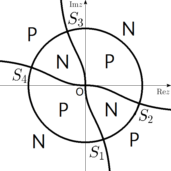
Figure 1. Signs of $\mathrm{Re}\,\varphi$

The signs of $\mathrm{Re}\,\varphi$ are shown in Figure 1: P and N stand for ’positive’ and ’negative’ respectively and $S_{j}$’s are the saddle points. Let $\Sigma$ be the contour (including the dotted and dashed parts) in Figure 2. The + signs indicate the plus side. The black squares are the poles $\pm z_{s},\pm\bar{z}_{s}^{-1}$ in (4.16) and (4.17). The small circles are centered at $\pm z_{j}$ and $\pm\bar{z}_{j}^{-1}$ for some $j\neq s$. We can bend $\Sigma$ so that the black squares and the small circles are in $\Omega_{1}\cup\Omega_{2}.$ There may be more quartets of small circles, but they are omitted in the figure. The orientations of the small circles are irrelevant because the jump matrices along them are exponentially close to the identity matrix.

The large circle is $\tilde{C}$. The union of the quartet(s) of the small circles is called $C^{\circ}$. The dotted part and the dashed part are called $L$ and $L^{\prime}$ respectively. We have $\Sigma=\tilde{C}\cup C^{\circ}\cup L\cup L^{\prime}$. Notice that $\mathrm{Re\,\varphi>0}$ on $L\setminus\left\{\textrm{the saddle points}\right\}$ and that $\mathrm{Re\,\varphi<0}$ on $L^{\prime}\setminus\left\{\textrm{the saddle points}\right\}$.

On each arc joining adjacent saddle points, we have the decomposition

$$\rho=R+h_{I}+h_{II},\;\bar{\rho}=\bar{R}+\bar{h}_{I}+\bar{h}_{II}.$$

This is a ’curved version’ of the decomposition in [8] and its construction is a variant of that given in [19, 20]. Here we just state what is necessary to understand the present paper. The leading parts are $R$ and $\bar{R}$ and the limit of $R(z)$ and $\bar{R}(z)$ as $z$ tends to a saddle point along an arc coincides with that of $\rho(z)$ and $\bar{\rho}(z)$ respectively. The other parts, $h_{I},h_{II},\bar{h}_{I}$ and $\bar{h}_{II}$ are small in the following sense. First, $|e^{-2\varphi}h_{I}|$ and $|e^{2\varphi}\bar{h}_{I}|$ are estimated by any negative power of $t$. Second, $h_{II}$ and $R$ (resp. $\bar{h}_{II}$ and $\bar{R}$ ) can be analytically continued to $\left\{\text{\text{Re\,}}\varphi>0\right\}$ (resp. $\left\{\text{\text{Re\,}}\varphi<0\right\}$) and $|e^{-2\varphi}h_{II}|$ (resp. $|e^{2\varphi}\bar{h}_{II}|$ ) is estimated by any negative power of $t$ on $L$ (resp. $L^{\prime}$). Lastly, $|e^{-2\varphi}R|$ (resp. $|e^{2\varphi}\bar{R|}$) decay exponentially on $L$ (resp. on $L^{\prime}$) except in small neighborhoods of the saddle points.

Figure 2. the contour $\Sigma$

We introduce the following matrices:

$$b_{+}^{0}=\delta_{+}^{\mathrm{ad}\sigma_{3}}e^{-(\varphi+d)\mathrm{ad}\sigma_{3}}\begin{bmatrix}1&\quad-h_{I}\\ 0&\quad 1\end{bmatrix},\; b_{+}^{a}=\delta_{+}^{\mathrm{ad}\sigma_{3}}e^{-(\varphi+d)\mathrm{ad}\sigma_{3}}\begin{bmatrix}1\;&\;-h_{II}-R\\ 0\;&\;1\end{bmatrix},$$

$$b_{-}^{0}=\delta_{-}^{\mathrm{ad}\sigma_{3}}e^{-(\varphi+d)\mathrm{ad}\sigma_{3}}\begin{bmatrix}1&\quad 0\\ \bar{h}_{I}&\quad 1\end{bmatrix},\; b_{-}^{a}=\delta_{-}^{\mathrm{ad}\sigma_{3}}e^{-(\varphi+d)\mathrm{ad}\sigma_{3}}\begin{bmatrix}1\;&\;0\\ \bar{h}_{II}+\bar{R}\;&\;1\end{bmatrix}.$$

Notice that $b_{\pm}^{a}$ can be analytically continued to $\left\{\pm\mathrm{Re\,}\varphi>0\right\}$. By (4.25), we have

$$\tilde{v}=(b_{-}^{a})^{-1}(b_{-}^{\circ})^{-1}b_{+}^{\circ}b_{+}^{a}$$ (5.1)

on any of the arcs. Set $b_{-}^{\sharp}=I,b_{-}^{0},b_{-}^{a}$ and $b_{+}^{\sharp}=b_{+}^{a},b_{+}^{0},I$ on $L,\tilde{C},L^{\prime}$ respectively. On $\Sigma\setminus C^{\circ}$, we set

$$v^{\sharp}=v^{\sharp}(z)=(b_{-}^{\sharp})^{-1}b_{+}^{\sharp}.$$

We have $v^{\sharp}=b_{+}^{a},(b_{-}^{0})^{-1}b_{+}^{0},(b_{-}^{a})^{-1}$ on $L,\tilde{C},L^{\prime}$ respectively. On the remaining part $C^{\circ}$, let $v^{\sharp}$ be equal to the jump matrices in (4.14) and (4.15). As a replacement for $\tilde{m}$ in Proposition 13, or rather $\tilde{m}\Delta^{-1}$ in (4.22), (4.14)-(4.18), we define a new unknown matrix $m^{\sharp}$ by

$$m^{\sharp} =\tilde{m}\Delta^{-1}, z\in\Omega_{1}\cup\Omega_{2},$$ (5.2)

$$=\tilde{m}\Delta^{-1}(b_{-}^{a})^{-1}, z\in\Omega_{3}\cup\Omega_{4},$$ (5.3)

$$=\tilde{m}\Delta^{-1}(b_{+}^{a})^{-1}, z\in\Omega_{5}\cup\Omega_{6}.$$ (5.4)

It is the unique solution to the Riemann-Hilbert problem

$$m_{+}^{\sharp}(z)=m_{-}^{\sharp}(z)v^{\sharp}(z),\hskip 11.99998ptz\in\Sigma,$$ (5.5)

$$\mathrm{Res}(m^{\sharp};\pm z_{s})=\lim_{z\to\pm z_{s}}m^{\sharp}(z)\Delta(z_{s})I_{\mathrm{\mathrm{res}}}(z_{s})\Delta(z_{s})^{-1},$$ (5.6)

$$\mathrm{Res}(m^{\sharp};\pm\bar{z}_{s}^{-1})=\lim_{z\to\pm\bar{z}_{s}^{-1}}m^{\sharp}(z)\Delta(\bar{z}_{s}^{-1})I_{\mathrm{\mathrm{res}}}(\bar{z}_{s}^{-1})\Delta(\bar{z}_{s}^{-1})^{-1},$$ (5.7)

$$m^{\sharp}(z)\to I\hskip 11.99998pt\mbox{as\;}z\to\infty.$$ (5.8)

See (4.20)-(4.21) for concrete expressions of matrices in (5.6)-(5.7). We shall employ $w_{\pm}^{\sharp}=\pm(b_{\pm}^{\sharp}-I)$, $w^{\sharp}=w_{+}^{\sharp}+w_{-}^{\sharp}$ . We have $v^{\sharp}=(I-w_{-}^{\sharp})^{-1}(I+w_{+}^{\sharp})=(I+w_{-}^{\sharp})(I+w_{+}^{\sharp}).$ Notice that $v^{\sharp}(z)$ is defined on $C^{\circ}$ in terms of $I_{\mathrm{exp}}^{\pm}(z;z_{j})$ and $I_{\mathrm{exp}}^{\pm}(z;\bar{z}_{j}^{-1})$. It is exponentially close to $I$ on $C^{\circ}$ as $t\to\infty$.

Let us derive a reconstruction formula in terms of $m_{21}^{\sharp}$. Near $z=0$, we have $m_{21}^{\sharp}(z)=\tilde{m}_{21}(z)\delta(z)^{-1}$, $\tilde{m}_{21}(z)=\hat{m}_{21}(z)\delta(0)T(z)^{-1}T(\infty)^{-1}$, $\hat{m}_{21}(z)=m_{21}(z)$. Therefore we obtain

$$m_{21}(z)=\tilde{m}{}_{21}(z)\delta(0)^{-1}T(\infty)T(z)=m_{21}^{\sharp}(z)\delta(0)^{-1}\delta(z)T(\infty)T(z).$$

Set $p_{s}=T(0)T(\infty)$. Then we have

$$p_{s}=\prod_{k>s}\,z_{k}^{2}\bar{z}_{k}^{-2},\quad|p_{s}|=1.$$ (5.9)

Since $\delta(z)$ and $T(z)$ are even functions, we get

$$R_{n}(t)=-\left.\frac{\,d}{\,dz}m(z)_{21}\right|_{z=0}=-T(0)T(\infty)\frac{\,dm_{21}^{\sharp}}{\,dz}(0)=-p_{s}\frac{\,dm_{21}^{\sharp}}{\,dz}(0).$$ (5.10)

6. Modified Cauchy kernel and the Beals-Coifman formula

Set

$$g(\zeta,z;a)=\frac{(z-a)(z+a)}{(\zeta-a)(\zeta+a)(\zeta-z)}=\frac{1}{\zeta-z}-\frac{z+a}{2a(\zeta-a)}+\frac{z-a}{2a(\zeta+a)}.$$

We have $g(\zeta,\pm a;a)=0$. Next set $h_{1}(\zeta,z)=g(\zeta,z;\bar{z}_{s}^{-1}),\,h_{2}=g(\zeta,z;z_{s})$. We have $h_{1}(\zeta,\pm\bar{z}_{s}^{-1})=h_{2}(\zeta,\pm z_{s})=0.$ We introduce the modified Cauchy kernel

$$\Omega(\zeta,z)=\frac{1}{2\pi i}\begin{bmatrix}h_{1}(\zeta,z)&0\\ 0&h_{2}(\zeta,z)\end{bmatrix}.$$

For any $2\times 2$ matrix $f=f(z)$, the second columns of $(f\Omega)(\pm z_{s})$ and the first columns of $(f\Omega)(\pm\bar{z}_{s}^{-1})$ are zero for any $\zeta$. We define the modified Cauchy operator $C^{\Omega}$ by $(C^{\Omega}f)(z)=\int_{\Sigma}f(\zeta)\Omega(\zeta,z)\,d\zeta$. We have

$$(C^{\Omega}f)(\zeta,\pm z_{s})=\begin{bmatrix}*&0\\ &0\end{bmatrix},$$ (6.1)

$$(C^{\Omega}f)(\zeta,\pm\bar{z}_{s}^{-1})=\begin{bmatrix}0&*\\ 0&*\end{bmatrix}.$$ (6.2)

The boundary values of $(C^{\Omega}f)(z)$ on $\Sigma$ are denoted by

$$(C_{\pm}^{\Omega}f)(z)=\int_{\Sigma}f(\zeta)\Omega(\zeta,z_{\pm})\,d\zeta=\lim_{\genfrac{}{}{0.0pt}{}{z^{\prime}\to z}{z^{\prime}\in\{\pm\textrm{\scriptsize-side of }\Sigma\}}}\int_{\Sigma}f(\zeta)\Omega(\zeta,z^{\prime})\,d\zeta,\;z\in\Sigma.$$

We have $C_{+}^{\Omega}-C_{-}^{\Omega}=\mathrm{identity}$. We introduce the modified Beals-Coifman operator $C_{w^{\sharp}}^{\Omega}\colon L^{2}(\Sigma)\to L^{2}(\Sigma)$ by

$$C_{w^{\sharp}}^{\Omega}f=C_{+}^{\Omega}(fw_{-}^{\sharp})+C_{-}^{\Omega}(fw_{+}^{\sharp})$$ (6.3)

for a $2\times 2$ matrix-valued function $f$.

Let $\mu^{\sharp}$ be the solution to the equation

$$\mu^{\sharp}=m_{0}^{\sharp}+C_{w^{\sharp}}^{\Omega}\mu^{\sharp}.$$ (6.4)

Here $m_{0}^{\sharp}$ is obtained from $m_{0}$ by replacing $C_{1}(0)$ with $\delta(0)\delta(z_{s})^{-2}T(z_{s})^{-2}C_{s}(0)$ in Proposition 5. See (4.20) and (4.21). We have $\mu^{\sharp}=(1-C_{w^{\sharp}}^{\Omega})^{-1}m_{0}^{\sharp}$ (the resolvent exists as is proved in the next section), and

$$m^{\sharp}(z)=m_{0}^{\sharp}(z)+\int_{\Sigma}\mu^{\sharp}(\zeta)w^{\sharp}(\zeta)\Omega(\zeta,z),\;z\in\mathbb{C}\setminus\left(\Sigma\cup\left\{\pm z_{s},\pm\bar{z}_{s}^{-1}\right\}\right)$$ (6.5)

is the unique solution to the Riemann-Hilbert problem (5.5)-(5.8). Indeed, the pole conditions (5.6)-(5.7) follow from (4.20), (4.21) and (6.1)-(6.2). On the other hand, (5.5) is satisfied because

$$m_{+}^{\sharp} =m_{0}^{\sharp}+C_{+}^{\Omega}(\mu^{\sharp}w^{\sharp})=m_{0}^{\sharp}+C_{+}^{\Omega}(\mu^{\sharp}w_{+}^{\sharp})+C_{+}^{\Omega}(\mu^{\sharp}w_{-}^{\sharp})$$

$$=m_{0}^{\sharp}+\mu^{\sharp}w_{+}^{\sharp}+C_{-}^{\Omega}(\mu^{\sharp}w_{+}^{\sharp})+C_{+}^{\Omega}(\mu^{\sharp}w_{-}^{\sharp})$$

$$=m_{0}^{\sharp}+C_{w^{\sharp}}^{\Omega}(\mu^{\sharp})+\mu^{\sharp}w_{+}^{\sharp}=\mu^{\sharp}+\mu^{\sharp}w_{+}^{\sharp}=\mu^{\sharp}b_{+}^{\sharp}$$

and similarly $m_{-}^{\sharp}=\mu^{\sharp}b_{-}^{\sharp}$. By substituting (6.5) into (5.10), we find that

$$R_{n}(t) =p_{s}\biggl{[}\mathrm{BS}\left(n,t;z_{s},\delta(0)\delta(z_{s})^{-2}T(z_{s})^{-2}C_{s}(0)\right)+E_{n}(t)\biggr{]},$$

$$E_{n}(t) =-\int_{\Sigma}z^{-2}\left[\bigl{(}(1-C_{w^{\sharp}}^{\Omega})^{-1}m_{0}^{\sharp}\bigr{)}(z)w^{\sharp}(z)\right]_{21}\frac{\,dz}{2\pi i}$$

$$\quad\,+\int_{\Sigma}\frac{1}{(z-\bar{z}_{s}^{-1})(z+\bar{z}_{s}^{-1})}\left[\bigl{(}(1-C_{w^{\sharp}}^{\Omega})^{-1}m_{0}^{\sharp}\bigr{)}(z)w^{\sharp}(z)\right]_{21}\frac{\,dz}{2\pi i}.$$ (6.6)

7. Estimates

In this section we prove the existence of the resolvent $(1-C_{w^{\sharp}}^{\Omega})^{-1}\colon L^{2}(\Sigma)\to L^{2}(\Sigma)$ and give an estimate on the error term $E_{n}(t)$ in (6.6). Let $C_{\pm}$ be the boundary values of the usual Cauchy integrals. We introduce the Beals-Coifman operator $C_{w^{\sharp}}\colon L^{2}(\Sigma)\to L^{2}(\Sigma)$ by

$$C_{w^{\sharp}}f=C_{+}(fw_{-}^{\sharp})+C_{-}(fw_{+}^{\sharp})$$

for a $2\times 2$ matrix-valued function $f$.

Proposition 15.

The resolvents $(1-C_{w^{\sharp}})^{-1},(1-C_{w^{\sharp}}^{\Omega})^{-1}\colon L^{2}(\Sigma)\to L^{2}(\Sigma)$ exist for any sufficiently large $t$.

Proof.

The existence of $(1-C_{w^{\sharp}}^{\Omega})^{-1}$ follows from that of $(1-C_{w^{\sharp}})^{-1}$, because the difference $C_{w^{\sharp}}^{\Omega}-C_{w^{\sharp}}$ is infinitely small for large $t$. The proof is as follows. We see that $\left(C_{w^{\sharp}}^{\Omega}-C_{w^{\sharp}}\right)f$ consists of terms like

$$\int_{\Sigma}\frac{\mathrm{const.}fw_{\pm}^{\sharp}}{\zeta\pm z_{s}}d\zeta,\,\int_{\Sigma}\frac{\mathrm{const.}fw_{\pm}^{\sharp}}{\zeta\pm\bar{z}_{s}^{-1}}d\zeta$$

and that $\pm z_{s},\pm\bar{z}_{s}^{-1}\not\not\in\Sigma$. Since the $L^{2}(\Sigma)$-norm of $w_{\pm}^{\sharp}$ is $O(t^{-1/4})$ ([19, §7.2]), the $L^{\infty}(\Sigma)$-norm of $\left(C_{w^{\sharp}}^{\Omega}-C_{w^{\sharp}}\right)f$ is $O(t^{-1/4})\times\|f\|_{L^{2}(\Sigma)}$. Since $\Sigma$ is bounded, the $L^{2}(\Sigma)$-norm of $\left(C_{w^{\sharp}}^{\Omega}-C_{w^{\sharp}}\right)f$ is also $O(t^{-1/4})\times\|f\|_{L^{2}(\Sigma)}$.

Next we show the existence of $(1-C_{w^{\sharp}})^{-1}$. Since $\sup_{C^{\circ}}|w_{\pm}^{\sharp}|=O(t^{-N})$ for any $N$, we have only to prove that $(1-C_{w^{\sharp}})^{-1}\colon L^{2}(\Sigma\setminus C^{\circ})\to L^{2}(\Sigma\setminus C^{\circ})$ exists. Here we abuse the notation $C_{w^{\sharp}}$ to mean an operator on $L^{2}(\Sigma\setminus C^{\circ})$. Then the necessary argument is similar to [19, §9, §11]. We encounter the matrix

$$V=e^{-((iz^{2})/4)\mathrm{ad}\,\sigma_{3}}\begin{bmatrix}1&-\bar{r}(S_{j})\\ -r(S_{j})&1+|r(S_{j})|^{2}\end{bmatrix}=\begin{bmatrix}1&-\bar{r}(S_{j})e^{-iz^{2}/2}\\ -r(S_{j})e^{iz^{2}/2}&1+|r(S_{j})|^{2}\end{bmatrix}$$

instead of $v^{e,\phi}(z)$ at the bottom of [19, p.796]. We have only to prove the existence of the resolvent of the Beals-Coifman operator in $L^{2}(\mathbb{R})$ associated with it. Now $|r(S_{j})|$ is not necessarily less than 1. The simple argument based on the Neumann series as in [8, (3.94)] and [19, p.797] is not valid. We can resort to [7, Lemma 5.9] instead. It implies the existence of $(1-C_{v^{\mathrm{DP}}})^{-1}$ in $L^{2}(\mathbb{R})$, where

$$v^{\mathrm{DP}}=v^{\mathrm{DP}}(z)=\begin{bmatrix}1+|a|^{2}&\bar{a}e^{i\theta}\\ ae^{-i\theta}&1\end{bmatrix},\,\theta=-z^{2}/2,\,a\colon\text{const.},$$

and $C_{v^{\mathrm{DP}}}$ is the Beals-Coifman operator associated with any factorization of $v^{\mathrm{DP}}$. Let $\mathbb{R}^{\mathrm{rev}}$ be the contour obtained by reversing the orientation of $\mathbb{R}$. By [9, Proposition 2.8], we have

$$C_{v^{\mathrm{DP}}}=C_{\left(v^{\mathrm{DP}}\right)^{-1}}\quad\text{in}\,L^{2}(\mathbb{R})=L^{2}(\mathbb{R}^{\mathrm{rev}}).$$

Notice that $\mathbb{R}^{\mathrm{rev}}$ can be identified with the conventionally oriented real axis of another copy of of $\mathbb{C}$ via $\mathbb{C}_{z}\to\mathbb{C}_{w},z\mapsto w:=-z$ and that we have $dz/(z-\xi)=dw/(w-\zeta),\zeta=-\xi$. Since $v^{\mathrm{DP}}(\xi)=v^{\mathrm{DP}}(\zeta)$, the resolvent $(1-C_{\left(v^{\mathrm{DP}}\right)^{-1}})^{-1}$ exists in $L^{2}(\mathbb{R})$. Notice that $\left(v^{\mathrm{DP}}\right)^{-1}$ has the same form as $V$. We have proved the existence of the resolvent of the Beals-Coifman operator associated with $V$. ∎

Next we can show $E_{n}(t)=O(t^{-1/2})$. The following proposition is a part of Theorem 11.

Proposition 16.

In the region $\mathrm{(-2<)tw}(z_{s})-d\leq n/t\leq\mathrm{tw}(z_{s})+d(<2)$, where $d$ is sufficiently small, the solution $R_{n}(t)$ differs from a soliton only by $O(t^{-1/2})$:

$$R_{n}(t)=\mathrm{BS}\left(n,t;z_{s},\delta(0)\delta(z_{s})^{-2}p_{s}T(z_{s})^{-2}C_{s}(0)\right)+O(t^{-1/2}).$$

Proof.

Lemma 7 implies that $p_{s}$ times a soliton is still a soliton. We have

$$p_{s}\mathrm{BS}\left(n,t;z_{s},\delta(0)\delta(z_{s})^{-2}T(z_{s})^{-2}C_{s}(0)\right)$$

$$\mathrm{=BS}\left(n,t;z_{s},\delta(0)\delta(z_{s})^{-2}p_{s}T(z_{s})^{-2}C_{s}(0)\right).$$

By using a change of variables (scaling) as in [19, pp.798-799], we can show that $E_{n}(t)$ in (6.6) satisfies $E_{n}(t)=O(t^{-1/2})$. The calculations about the parabolic cylinder functions only need minor changes. One important step relies on the fact that the determinant of the jump matrix is equal to $1$ ([8, pp.349-350]), which remains true for the focusing discrete NLS. ∎

Remark 17.

The proof of the solitonless case of Theorem 18 is almost the same as that of the defocusing case ([19]). The calculations about the parabolic cylinder functions only need minor changes. One important step relies on the fact that the determinant of the jump matrix is equal to $1$ ([8, pp.349-350]), which remains true.

One thing to be noted is that now $r(z)$ is accompanied by the factor $\bar{T}(z)^{2}.$ It has no effect when we consider quantities involving $|r(z)|^{2}$ because we have $|T(z)|=1$ on $C$. Although $C_{j}$’s are affected by $T(z)$, $q_{j}$’s are not. See [19, Theorem 3.1].

8. Other regions

In the preceding sections we considered the region $|n|<2t$. In this section, we consider two other regions following [20]. The equation (1.1) is invariant under the reflection $n\mapsto-n$. We may assume $n>0$ without loss of generality.

By using the argument of [20], we can show the following theorem.

Theorem 18.

Assume that $\mathrm{tw}(z_{s})=2$ for some eigenvalue $z_{s}$. Then in the region $2t-Mt^{1/3}<n<2t+M^{\prime}t^{1/3}\;(M>0)$, we have

$$R_{n}(t)=\mathrm{BS}\left(n,t;z_{s},p_{s}T(z_{s})^{-2}C_{s}(0)\right)+O(t^{-1/3})\quad\text{as}\;t\to\infty.$$

In the solitonless case, i.e. if $\mathrm{tw}(z_{j})\neq 2$ for any $j$, then the behavior is as follows: let $t_{0}$ be such that $\pi^{-1}\left[\arg r(e^{-\pi i/4})\overline{T(e^{-\pi i/4})}^{2}-2t_{0}\right]$ is an integer. Set $t^{\prime}=t-t_{0}$, $p^{\prime}=d+i(-4t^{\prime}+\pi n)/4$, $\alpha^{\prime}=[12t^{\prime}/(6t^{\prime}-n)]^{1/3}$, $q^{\prime}=-2^{-4/3}3^{1/3}(6t^{\prime}-n)^{-1/3}(2t^{\prime}-n)$ and $\hat{r}=r(e^{-\pi i/4})\overline{T(e^{-\pi i/4})}^{2}$. Then we have

$$R_{n}(t)=\frac{e^{2p^{\prime}-\pi i/4}\alpha^{\prime}}{(3t^{\prime})^{1/3}}u\Bigl{(}\frac{4q^{\prime}}{3^{1/3}};\hat{r},-\hat{r},0\Bigr{)}+O(t^{\prime-2/3}).$$

Here $u(s;\mathrm{p,q,r})$ is a solution of the Painlevé II equation $u^{\prime\prime}(s)-su(s)-2u^{3}(s)=0$. Its parametrization is given in [8] (and is repeated in [20]).

Proof.

In order to prove the soliton case, derive a variant of (6.5) adapted to this case. To estimate the integral, follow the argument of [20, §8]. The calculation is somewhat different from the previous one. This is because we apply a scaling of order $t^{-1/3}$ as in [20, §4]. Notice that values of $\delta(z)$ are absent in the third argument of $\mathrm{BS}$. It is because the signature table of the phase function is good enough from the beginning and the $\Delta(z)$-conjugation is unnecessary. Indeed, in the proof of [7, Lemma 5.9], what matters is the fact that the jump matrix is strictly positive definite ([7, Lemma 5.2]).

The proof of the existence of resolvents must be modified because the modulus of the reflection coefficient is not necessarily less than $1$. We can employ a variant of Lemma 5.9 of [7]. We replace the phase with $-4i(z^{3}-\textrm{const}.z)$. The change of the signature table does not spoil the proof. It rather simplifies the argument since one can employ a simpler factorization without introducing the function $\delta$ of [7, (5.12)]. Moreover, what matters in the proof of [7, Lemma 5.9] is the fact that the jump matrix is strictly positive definite and phase functions need not to be quadratic.

In the solitonless case, we have to modify the argument of [20] slightly. The quantity $d=\frac{1}{2}\log\delta(0)$ can be dealt with simulaneously with $p^{\prime}.$

Next, notice that $\begin{bmatrix}1-|r|^{2}&-\bar{r}\\ r&1\end{bmatrix}$ (in the expression of $v$), $\begin{bmatrix}1&0\\ r&1\end{bmatrix}$ (in the expression of $J_{23}$) and $\begin{bmatrix}1&-\bar{r}\\ 0&1\end{bmatrix}$ (in the expression of $J_{67}$) in [20] must be replaced with $\begin{bmatrix}1+|r|^{2}&-\bar{r}T^{2}\\ r\bar{T}^{2}&1\end{bmatrix}$, $\begin{bmatrix}1&0\\ r&1\end{bmatrix}$ and $\begin{bmatrix}1&-\bar{r}T^{2}\\ r\bar{T}^{2}&1\end{bmatrix}$ in the present paper. We want to set

$$\mathrm{p}=r(e^{-\pi i/4})\overline{T(e^{-\pi i/4})}^{2},\mathrm{q}=-r(e^{-\pi i/4})\overline{T(e^{-\pi i/4})}^{2}=-\bar{r}(e^{-\pi i/4})T(e^{-\pi i/4})^{2},$$

where $\mathrm{\mathrm{p}}$ and $\mathrm{\mathrm{q}}$ are the parameters in [8, (5.33)] or [20, Appendix]. Notice that $r(e^{-\pi i/4})\overline{T(e^{-\pi i/4})}^{2}$ must be real. It is possible to reduce our problem to such a case by a time shift like the one in [20, §5]. In [20], $r(e^{-\pi i/4})$ was purely imaginary and $T$ was not present. ∎

Next we consider the region $|n/t|>2$.

Theorem 19.

In $2<\mathrm{tw}(z_{s})-d\leq n/t\leq\mathrm{tw}(z_{s})+d$, where $d$ is sufficiently small, we have

$$R_{n}(t)=\mathrm{BS}\left(n,t;z_{s},p_{s}T(z_{s})^{-2}C_{s}(0)\right)+O(n^{-k})\quad\text{as}\;|n|\to\infty$$

for any positive integer $k$.

In the solitonless case, i.e. if $\mathrm{tw}(z_{j})\not\in[n/t-d,n/t+d]$ for any $j$, then

$$R_{n}(t)=O(n^{-k})\quad\text{as}\;|n|\to\infty$$

for any positive integer $k$.

Proof.

In order to prove the former case, derive a variant of (6.5) adapted to this case. To estimate the integral, follow the argument of [20, §8]. The latter case can be proved in the same way as [20, §8]. ∎

Appendix: Counter-examples

We show that $a(z)$ may vanish on the unit circle $|z|=1$ and that it may have double zeros. Moreover, we prove that there may be two eigenvalues corresponding to the same velocity.

Assume that $R_{n}=0$ for $n\neq 0,1,2$. Then we have ([3, (3.2.24)])

$$\phi_{n}(z,t)=z^{n}\begin{bmatrix}1\\ 0\end{bmatrix}\,(n\leqq 0),\;\psi_{n}(z,t)=z^{-n}\begin{bmatrix}0\\ 1\end{bmatrix}\,(n\geqq 3).$$ (8.1)

The $n$-part (2.2) implies

$$\phi_{3}(z,t)=\mathcal{M}_{2}\mathcal{M}_{1}\mathcal{M}_{0}\begin{bmatrix}1\\ 0\end{bmatrix}=\begin{bmatrix}z^{3}-(R_{0}\bar{R}_{1}+R_{1}\bar{R}_{2})z-R_{0}\bar{R}_{2}z^{-1}\\ \text{omitted}\end{bmatrix}.$$ (8.2)

We have the Wronskian formula ([3, (3.2.64c)])

$$a(z)=c_{n}W(\phi_{n},\psi_{n}),\;c_{n}=\prod_{k=n}^{\infty}(1+|R_{n}|^{2})\geqq 1.$$

Here $n$ is arbitrary. We apply it to the case $n=3$. We employ (8.2) and $\psi_{3}$ is calculated by using (8.1). We set $R_{1}=1$. Then we obtain

$$a(z)=c_{3}z^{-4}f(z^{2}),\;f(x)=x^{2}-(R_{0}+\bar{R}_{2})x-R_{0}\bar{R}_{2}.$$

It is elementary that $f(x)$ can have any pair of complex numbers, say $x_{1}$ and $x_{2}$, as zeros if $R_{0}$ and $\bar{R}_{2}$ are suitably chosen. It is enough to choose $R_{0}$ and $\bar{R}_{2}$ so that

$$R_{0}+\bar{R}_{2}=x_{1}+x_{2},\;R_{0}\bar{R}_{2}=-x_{1}x_{2}.$$

The zeros of $a(z)$ are $\pm x_{1}^{1/2},\pm x_{2}^{1/2}$. If we choose $x_{1}$ and $x_{2}$ properly, the following three phenomena can occur:

• $a(z)$ has zeros on $|z|=1$.

• $a(z)$ has double zeros.

• $\mathrm{tw}(x_{1}^{1/2})=\mathrm{tw}(x_{2}^{1/2})$.

Of course, a general theory of Darboux transformations is preferable.