Kinematic Dynamo, Supersymmetry Breaking, and Chaos

Abstract

The kinematic dynamo (KD) describes the growth of magnetic fields generated by the flow of a conducting medium in the limit of vanishing backaction of the fields onto the flow. The KD is therefore an important model system for understanding astrophysical magnetism. Here, the mathematical correspondence between the KD and a specific stochastic differential equation (SDE) viewed from the perspective of the supersymmetric theory of stochastics (STS) is discussed. The STS is a novel, approximation-free framework to investigate SDEs. The correspondence reported here permits insights from the STS to be applied to the theory of KD and vice versa. It was previously known that the fast KD in the idealistic limit of no magnetic diffusion requires chaotic flows. The KD-STS correspondence shows that this is also true for the diffusive KD. From the STS perspective, the KD possesses a topological supersymmetry and the dynamo effect can be viewed as its spontaneous breakdown. This supersymmetry breaking can be regarded as the stochastic generalization of the concept of dynamical chaos. As this supersymmetry breaking happens in both the diffusive and the non-diffusive case, the necessity of the underlying SDE being chaotic is given in either case. The observed exponentially growing and oscillating KD modes prove physically that dynamical spectra of the STS evolution operator that break the topological supersymmetry exist with both, real and complex ground state eigenvalues. Finally, we comment on the non-existence of dynamos for scalar quantities.

I Introduction

The magnetohydrodynamical dynamo has a long scientific history and many important theoretical insights on it have already been provided (Bullard and Gellman, 1954; Parker, 1955; Braginskiy, 1964; Parker, 1970; Krause and Raedler, 1980; RÃŒdiger, 2004, and others). Roughly speaking, the magnetic dynamo phenomenon is the ability of a moving conducting medium to generate and/or to sustain a magnetic field. This phenomenon is wide-spread in astrophysical objects like galaxies (Parker, 1992; Beck et al., 1994; Subramanian, 1998; Beck, 2007, for example), galaxy clusters (Ruzmaikin et al., 1989; Dolag et al., 2002; Enßlin and Vogt, 2006; Vazza et al., 2014), stars (Parker, 1975; Glatzmaier, 1984; Raedler, 1986; Charbonneau and MacGregor, 2001; Spruit, 2002; Braithwaite, 2006; Browning, 2008), and planets including Earth (Bullard and Gellman, 1954; Parker, 1955; Taylor, 1963; Braginskiy, 1964; Raedler, 1986; Kuang and Bloxham, 1997). System-sized ordered fields can be observed in objects with large-scale ordered flows such as those occurring in rotating galaxies, stars, and planets, and are usually attributed to the action of the so-called large-scale, mean-field, or $\alpha-\mbox{$\omega$}$ dynamo. Systems without a large-scale flow pattern can also harbor dynamos driven by turbulent fluid motions. These are called small-scale, fluctuating, or turbulent dynamos and are believed to maintain the magnetic fields in galaxy clusters. Although the theory of dynamos is relatively mature, it still provides a field of active and interesting research.

Dynamo theory addresses two different regimes. The first one is the kinematic dynamo (KD, (Braginskiy, 1964; Lerche, 1971; Roberts, 1972; Li et al., 2010a)). In this regime, the amplified magnetic field is too weak to affect the flow of the conducting medium. This regime is realized, for example, in the early stages of galaxy formation. The other regime is the nonlinear dynamo. Here, the backaction of a sufficiently strongfield on the flow is not negligible anymore. Such backactions lead eventually to a saturated dynamo state, with an average stationary magnetic energy linked to the kinetic energy of the flow. This regime seems to be realized in the magnetic fields in developed galaxies and galaxy clusters. This paper, however, focuses solely on the KD limit.

It is known (see, e.g., Ref. (Motter, 2014) and references therein) that the KD in the idealistic diffusionless case requires chaotic underlying flows of matter (see, e.g., Ref. (Ott, 2007) and references therein). It was not known until this work whether this relation also holds if magnetic diffusivity is present. Establishing the chaos-KD relation under diffusivity requires a rigorous mathematical generalization of the concept of deterministic chaos to stochastic flows, which was missing so far. The recently found supersymmetric theory of stochastics (STS) closes this gap (Ovchinnikov, 2013, 2014).

The STS is an approximation-free theory of stochastic differential equations (SDEs). Instead of investigating the ensemble of stochastic trajectories generated by an SDE, the STS analyzes the actions (or pullbacks) induced by these trajectories on the elements of the exterior algebra of the phase space – the differential forms of various degrees, in the following called wavefunctions. These wavefunctions can be averaged over the stochastic noise configurations, as the exterior algebra, together with the SDE-induced actions on it, is a linear space in which the stochastic averaging is legitimate. In contrast, the concept of the stochastically averaged trajectories themselves can not be straightforwardly defined for non-linear phase spaces. The stochastically averaged SDE-defined pullback, i.e., the stochastic evolution operator, provides a complete picture of all aspects of the stochastic dynamics. For example, the temporal evolution of an initial $\delta$-functional probability distribution in the phase space can be explicitly constructed from it.

The KD-STS correspondence that we want to highlight here emerges from the identification of the fluid flow and the magnetic fields of the KDs with the flow vector field of an SDE and the (non-supersymmetric) two-forms (or 1-forms in case one described the magnetic field in terms of the magnetic vector potential) respectively. This connection permits the transfer of insights obtained within the STS to the KD theory and vice versa.

In the STS, all SDEs possess a topological (or De Rahm) supersymmetry. This means that the stochastic evolution operator commutes with the so-called exterior derivative or De Rahm operator, $\hat{d}$, of the exterior algebra (see Sec. II). As a mathematical consequence of this (see Sec. III.2), all eigenstates of a time-independent stochastic evolution operator of a stationary SDE are divided into the finite number (one for each De Rahm cohomology class) of the zero-eigenvalue (or steady-state) supersymmetric singlets and the infinite number of the non-supersymmetric doublets with arbitrary, but bounded from below eigenvalues.

If there are growing eigenstates, the fastest growing eigenstate must be identified as the ground state of the model. Indeed, if an initial wavefunction has a contribution by such an eigenstate, this fastest growing eigenstate will dominate over the initial wavefunction after a sufficiently long period. The supersymmetry is said to be broken spontaneously in such a situation because this ground state has non-zero eigenvalue and thus is non-supersymmetric.

KDs are known to show growing magnetic fields (Ott, 2007). Thus, the supersymmetry of their corresponding SDEs is spontaneously broken. In other words, the existence of the growing modes of the KD is the physical proof that the supersymmetry breaking spectra of the STS evolution operator are realizable. Moreover, the well established existence of the oscillating fastest growing KD modes (Baryshnikova and Shukurov, 1987; Ruzmaikin et al., 1988; Li et al., 2010b) demonstrate that the STS spectra with complex ground state eigenvalues are also realizable.

The concept of spontaneous supersymmetry breaking in the STS, required for the existence of the growing KD modes, can actually be identified with the stochastic generalization of the concept of deterministic chaos (Ovchinnikov, 2013). For spontaneously broken symmetries, the Goldstone theorem predicts the existence of gapless Goldstone-Nambu excitations, which have infinite characteristic time-scales. This long-term dynamical behavior can be regarded as the manifestation of the ubiquitously observed “chaotic or dynamical long-range order” that reveals itself in such phenomena as the butterfly effect (Motter, 2014), $\nicefrac{{1}}{{f}}$ noise (Dutta and Horn, 1981), and the power-law statistics of various sudden (or instantonic) processes like solar flares (Aschwanden, 2011), earthquakes (Gutenberg and Richter, 1955), and neuronal avalanches (Beggs and Plenz, 2003). Therefore, the long-range phenomena associated with the presence of the dynamical long-range order must also be present in the KD systems, which is one of the interesting conclusions that can be drawn from the KD-STS correspondence discussed in this paper.

The structure of the paper is as follows: In Sec. II, it is demonstrated that the dynamical (stochastic) equations of the stationary KD possess topological supersymmetry. In Sec. III, the SDE corresponding to the KD effect is established and the relation of STS to growing KD modes, chaos, and supersymmetry breaking is elaborated. Sec. IV concludes the paper.

II Supersymmetry of the Kinematic Dynamo Equation

Temporal evolution of the magnetic field within the KD effect is governed by the induction equation:

$$\partial_{t}B = \partial\times\left(v\times B\right)+\eta\triangle B.$$ (1)

Here, $\partial_{t}\equiv\partial/\partial t$, $\partial=\{\partial_{i}\equiv\partial/\partial x^{i},x^{i}=x,y,z,i=1,2,3$}, is the gradient operator, $\triangle=\partial^{2}=\partial_{i}\partial_{i}$, is the Laplace operator, $\times$ denotes the vector product of two vectors so that $\partial\times$ is the curl of a vector, $B=\{B^{i},i=1,2,3\}$ is the magnetic field, $v=\{v^{i},i=1,2,3\}$ is the vector field of the underlying flow velocity of the conducting medium, and $\eta=1/(\sigma\mu)$ is the magnetic diffusivity with $\sigma$ and $\mu$ being the electrical conductivity and permeability. The first term in the r.h.s of Eq. (1) represents the well-known magnetohydrodynamical phenomenon of magnetic fields being frozen into the conducting medium, whereas the second term describes the magnetic field diffusion.

Our first goal is to translate Eq. (1) into the coordinate-free language of exterior algebra used by the STS. Instead of the vector $B$, we use differential forms of second degree to describe magnetic fields. Such 2-forms provide the coordinate-free representation of the same object,

$$F = \frac{1}{2!}F_{ij}dx^{i}\wedge dx^{j}=\hat{d}A.$$ (2)

Here, $A=A_{i}dx^{i}$ is the 1-form of the magnetic vector potential, $\hat{d}=dx^{i}\wedge\partial/\partial x^{i}$ is the exterior derivative or the De Rahm operator, and $\wedge$ is the wedge or antisymmetric product of differentials. In components, the antisymmetric contra-variant tensor, $F_{ij}$, called the magnetic field tensor, is given as:

$$F_{ij} = \partial_{i}A_{j}-\partial_{j}A_{i}=\epsilon_{ijk}B^{k}=\left(\begin{array}[]{ccc}0&B^{z}&-B^{y}\\ -B^{z}&0&B^{x}\\ B^{y}&-B^{x}&0\end{array}\right),$$

where $\epsilon_{ijk}$ is the antisymmetric Levi-Cevita tensor.

Eq. (1) in components is

$$\partial_{t}B^{i}=\epsilon^{ipq}\partial_{p}\epsilon_{qkl}v^{k}B^{l}+\eta\triangle B^{i}.$$

We work in the Eulcidian metric. Thus, lowering and raising the indices has no effect on the values of the components of the antisymmetric tensor, e.g., $\epsilon_{ijk}=\epsilon^{ijk}$. With the use of the following identity,

$$\epsilon_{qkl}\epsilon^{ipq}=\mathrm{det}\left(\begin{array}[]{cc}\delta_{k}^{i}&\delta_{k}^{p}\\ \delta_{l}^{i}&\delta_{l}^{p}\end{array}\right),$$ (4)

where $\delta_{j}^{i}$ is the Kronecker-delta and with $\partial_{i}B^{i}=0,$ Eq. (1) can be rewritten as:

$$\partial_{t}B^{i}=-\left(\partial_{j}v^{j}\right)B^{i}+B^{j}v_{{}^{\prime}j}^{i}+\eta\triangle B^{i},$$

where $v_{{}^{\prime}j}^{i}=\partial_{j}v^{i}$. Using now

$$B^{i}=\frac{1}{2}\epsilon^{ikl}F_{kl},$$

the induction equation can be further rewritten as:

$$\partial_{t}\frac{1}{2}\epsilon^{ikl}F_{kl} = -\partial_{j}v^{j}\frac{1}{2}\epsilon^{ikl}F_{kl}+\frac{1}{2}\epsilon^{jkl}F_{kl}v_{{}^{\prime}j}^{i}$$

$$+\eta\triangle\frac{1}{2}\epsilon^{ikl}F_{kl}.$$

Multiplying both sides of this Eq. by $\epsilon_{iab}$ and summing over index $i$, we get:

$$\partial_{t}F_{ab}=-\partial_{j}v^{j}F_{ab}+\frac{1}{2}\epsilon_{iab}\epsilon^{jkl}F_{kl}v_{{}^{\prime}j}^{i}+\eta\triangle F_{ab}.$$

With the help of the identity

$$\epsilon_{iab}\epsilon^{jkl}=\mathrm{det}\left(\begin{array}[]{ccc}\delta_{i}^{j}&\delta_{a}^{j}&\delta_{b}^{j}\\ \delta_{i}^{k}&\delta_{a}^{k}&\delta_{b}^{k}\\ \delta_{i}^{l}&\delta_{a}^{l}&\delta_{b}^{l}\end{array}\right),$$

one arrives at

$$\partial_{t}F_{ab} = -\partial_{j}v^{j}F_{ab}+\frac{1}{2}\left(2F_{ab}v_{{}^{\prime}j}^{j}-2F_{jb}v_{{}^{\prime}a}^{j}-2F_{aj}v_{{}^{\prime}b}^{j}\right)$$

$$+\eta\triangle F_{ab},$$

or

$$\partial_{t}F_{ab}=-\left(v^{j}\partial_{j}F_{ab}+v_{{}^{\prime}a}^{j}F_{jb}+F_{aj}v_{{}^{\prime}b}^{j}\right)+\eta\triangle F_{ab}.$$

Turning now to the coordinatee-free object $F$ in Eq. (2), Eq. (1) takes the form

$$\partial_{t}F = -\hat{H}_{\mathrm{KD}}F,\>\;\hat{H}_{\mathrm{KD}}=\hat{\mathcal{L}}_{v}-\eta\hat{\triangle},$$ (5)

where the Lie derivative along $v$ is defined as

$$\hat{\mathcal{L}}_{v} = v^{i}\partial_{i}+v_{{}^{\prime}j}^{i}dx^{j}\wedge\hat{\imath}_{i}.$$

Here, $\hat{\imath}_{i}$ is the interior multiplication acting on a differential form $\psi=\frac{1}{k!}\psi_{i_{1}...i_{k}}dx^{i_{1}}\wedge...\wedge dx^{i_{k}}$ as

$$\hat{\imath}_{i}\psi = \frac{1}{(k-1)!}\psi_{ii_{2}...i_{k}}dx^{i_{2}}\wedge...\wedge dx^{i_{k}}.$$

The resulting Eq. (5) is rather natural. As we already mentioned, the first term in the r.h.s. of Eq. (1) describes the infinitesimal temporal evolution of the magnetic field “frozen” into the conducting medium. This freezing of the magnetic field is the well-known magnetohydrodynamical effect. In the coordinate-free setting, the frozen field corresponds to the evolution solely due to the flow along $v$ and this evolution is given by the Lie derivative, which is also known as the physical derivative.

The next step towards STS is to establish the supersymmetric structure of the KD evolution operator, $\hat{H}_{\mathrm{KD}}$.

First, we recall the Cartan formula,

$$\hat{\mathcal{L}}_{v} = [\hat{d},\hat{\imath}_{v}],$$ (6)

where $\hat{\imath}_{v}=v^{i}\,\hat{\imath}_{i}$ the interior multiplication with $v$ and the square brackets denote the bi-graded commutator. This is defined by

$$[\hat{X},\hat{Y}] = \hat{X}\hat{Y}-(-1)^{\mathrm{deg}\hat{X}\mathrm{\cdot deg}\hat{Y}}\hat{Y}\hat{X},$$

where $\mathrm{deg}$ is the degree of the operator, i.e., the number of $dx$’s minus the number of $\hat{\imath}$’s. For example, $\mathrm{deg}\,\hat{d}=1$ and $\mathrm{deg}\,\hat{\imath}_{v}=-1$ so that the bi-graded commutator in Eq. (6) is actually an anti-commutator.

Second, the Laplace operator can be given by

$$\hat{\triangle} = -[\hat{d},\hat{d}^{\dagger}],$$ (7)

where $\hat{d}^{\dagger}=-\hat{\imath}_{i}\delta^{ij}\partial_{j}$ is the Hodge conjugate of the exterior derivative with respect to the Euclidian metric.

Substituting Eqs. (7) and (6) into Eq. (5), one finds the explicitly supersymmetric form of the KD evolution operator,

$$\hat{H}_{\mathrm{KD}} = [\hat{d},\hat{\bar{d}}],$$ (8)

where

$$\hat{\bar{d}} = \hat{\imath}_{v}+\eta\hat{d}^{\dagger}.$$

The notational similarity of the exterior derivative $\hat{d}$ and the evolution-defining $\hat{\bar{d}}$ is motivated by the fact that for a purely diffusive dynamics, with $\hat{H}=-\eta\hat{\triangle}$, these operators are the Hodge conjugates to each other (up to a diffusion constant) with respect to the Euclidian metric, $\hat{\bar{d}}=\eta\hat{d}^{\dagger}$.

We now show the supersymmetry of $\hat{H}_{\mathrm{KD}}$. We recall that due to the nil-potency of the exterior derivative, $\hat{d}^{2}=0$, one has

$$[\hat{d},[\hat{d},\hat{X}]] = 0,$$ (9)

for any $\hat{X}$. Thus, an immediate consequence of Eq. (9) and the “$\hat{d}$-exactness” of the KD evolution operator in Eq. (8), is that it commutes with $\hat{d}$:

$$[\hat{d},\hat{H}_{\mathrm{KD}}] = 0.$$ (10)

This suggests that $\hat{d}$ is a symmetry of the KD dynamics. Since $\hat{d}=dx^{i}\wedge\partial/\partial x^{i}$ removes a bosonic (commuting) variable (an $x^{i}$ is removed by $\partial/\partial x^{i}$) and replaces it by a fermionic one (an anti-commuting $dx^{i}\wedge$ is added) it converts bosonic variables into fermionic ones. Therefore, the symmetry of the evolution operator $\hat{H}_{\mathrm{KD}}$ with respect to $\hat{d}$ can be regarded as a supersymmetry since an exchange of a boson by a fermion in the wavefunction does not change its dynamics.

As a consequence of its supersymmetry conserving dynamics, the KD is described equivalently in terms of the magnetic field tensor and in terms of the vector potential in Eq. (2),

$$\partial_{t}A = -\hat{H}_{\mathrm{KD}}A$$

$$\Rightarrow\partial_{t}\hat{d}A = -\hat{d}\hat{H}_{\mathrm{KD}}A$$

$$\Rightarrow\partial_{t}\hat{d}A = -\hat{H}_{\mathrm{KD}}\hat{d}A$$

$$\Rightarrow\partial_{t}F = -\hat{H}_{\mathrm{KD}}F.$$ (11)

From a traditional KD perspective, it might come as a surprise that the magnetic field tensor and magnetic vector potential obey exactly the same evolution equation, despite being mathematically different, although related objects. From a STS perspective, this equivalence just shows the consistence of our calculations. In fact, the descriptions of the magnetic field evolution in terms of $A$ and $F$ must be equivalent. This suggests on its own that the exterior derivative (connecting $A$ and $F=\hat{d}A$) must be commutative with the evolution operator. Thus, we could just as well have guessed the existence of this supersymmetry from the very outset.

Note, however, that Eq. (8) not only implies the commutativity of the evolution operator with the exterior derivative, Eq. (10), it also implies that all the supersymmetric eigenstates have zero eigenvalue, as we discuss in the next section.

The close relation between supersymmetry, invariance under the action of $\hat{d}$, and algebraic topology, relations of topological sets with their boundaries, which we mentioned in the introduction, was first established in Ref. (Witten, 1982). This relation had resulted in the discovery of Witten-type topological or cohomological field theories (see, e.g., Refs. (Frenkel et al., 2007; Labastida, 1989; Witten, 1988a, b) and references therein, as well as Ref. (Birmingham et al., 1991) for a review). The STS that we are going to discuss next can be looked at as a member of this class of theories.

III Connection between the KD theory and the STS

III.1 Corresponding stochastic system

In this section, we will show that the stationary KD equation including magnetic diffusivity is the STS stochastic evolution operator of a certain SDE. To find this corresponding SDE, let us address here a more general SDE, establish its stochastic evolution operators, and compare it with $\hat{H}_{\mathrm{KD}}$. This general SDE can be thought of as one describing the trajectory of a test particle propagating along the fluid flow while its velocity is also subject to Gaussian white noise,

$$\dot{x}^{i}(t) = v^{i}(x(t))+(2\Theta)^{1/2}e_{a}^{i}(x(t))\xi^{a}(t).$$ (12)

Here, $x$ is the particle (or phase-space) position, $v=\{v^{i}\}$ is the stationary part of the flow vector field, $e_{a}(x)=\{e_{a}^{i}(x);i,a=1,2,3\}$ is a set of vector fields that can be characterized as the “prime vectors” of flow fluctuations at x and that are assumed position-dependent for now, $\xi^{a}(t)\in\mathbb{R}^{1}$ with $a\in\left\{1,2,3\right\}$ are the Gaussian white fluctuations with the standard stochastic averages,

$$\langle\xi^{a}(t)\rangle_{\text{noise}} = 0\text{ and }$$ (13)

$$\langle\xi^{a}(t)\xi^{b}(t^{\prime})\rangle_{\mathrm{noise}} = \delta^{ab}\delta(t-t^{\prime}),$$ (14)

and $\Theta$ is the intensity or temperature of these fluctuations. Getting a bit ahead, the flow vector field of the SDE corresponding to the KD equation will turn out to be the same as in the original KD problem. This is the reason why we do not introduce a new notation for the flow in Eq.12.

First, an evolution operator $M_{t^{\prime}t}^{*}$ is defined, which describes how the dynamics of the system acts on elements of the exterior algebra of the position (or phase) space. The elements of the exterior algebra form a Hilbert space, the space of differential forms of all degrees, $\varOmega(X)$. We recall that our magnetic field tensor and magnetic vector potential are among such elements, they are 2- and 1-forms respectively. Mathematically, $M_{t^{\prime}t}^{*}$ is the pullback of the inverse, finite-time evolution diffeomorphism. For a fixed noise configuration, this evolution operator is

$$M_{t^{\prime}t}^{*}=\mathcal{T}e^{-\int_{t^{\prime}}^{t}d\tau\mathcal{\hat{L}}_{v(\tau)}},$$ (15)

where $\mathcal{T}$ expresses chronological ordering of the terms to its right (see below). The time-dependent flow vector field is the entire r.h.s. of Eq. (12),

$$v(t)=v^{i}+(2\Theta)^{1/2}e_{a}^{i}\xi^{a}(t),$$

and the corresponding time dependent Lie derivative of this flow is

$$\mathcal{\hat{L}}_{v(t)}=\mathcal{\hat{L}}_{v}+(2\Theta)^{1/2}\xi^{a}(t)\mathcal{\hat{L}}_{e_{a}}.$$ (16)

Since the Lie derivative is linear in its argument, a stochastic term is just added to the time independent Lie derivative given by Eq. (6). The operator of the chronological ordering $\mathcal{T}$ is needed in Eq. (15) because in general instances of $\mathcal{\hat{L}}_{v(\tau)}$ at different times do not commute with each other. Eq. (15) follows immediately from one of the definitions of the Lie derivative, which is the infinitesimal pullback along a vector field.

Secondly, the finite-time evolution operator $M_{t^{\prime}t}^{*}$ is averaged over all the configurations of the stochastic noise:

$$\hat{M}_{tt^{\prime}}=\left\langle M_{t^{\prime}t}^{*}\right\rangle_{\text{noise}}.$$ (17)

As $M_{t^{\prime}t}^{*}$ is a linear operator acting on $\varOmega(X)$, the Hilbert space of all differential forms in which superpositions are possible, $\hat{M}_{tt^{\prime}}$ represents a mathematically meaningful average. This averaged finite-time evolution operator describes how wavefunctions evolve in time under the action of a dynamical system:

$$\psi(t)=\hat{M}_{tt^{\prime}}\psi(t^{\prime}),\,\psi\in\varOmega(X).$$ (18)

The infinitesimal stochastic evolution of the wave function can be given via the stochastic evolution equation

$$\partial_{t}\psi(t)=-\hat{H}\psi(t),$$ (19)

where the stochastic evolution operator (SEO) is defined by

$$\hat{H} = \lim_{\delta t\to 0}\frac{\hat{1}_{\Omega}-\hat{M}_{(t+\delta t)t}}{\delta t}.$$ (20)

STS investigates the evolution of the complete set of forms $\psi\in\Omega(X)$, whereas in the KD theory usually only the 2-forms $F\in\Omega^{2}(X)\subset\Omega(X)$ are of interest (or 1-forms $A\in\Omega^{1}(X)\subset\Omega(X)$ if one chooses to work with the vector potential). For example, the total probability density 3-form $\psi(t)=\rho(x,t)\,dx^{1}\wedge dx^{2}\wedge dx^{3}\in\varOmega^{3}(X)$ to find the system in a specific phase space volume around location $x$ at time $t$ evolves according to Eq. (19) restricted to $\varOmega^{3}(X)$. The correspondingly restricted SEO is the conventional Fokker-Planck operator and will here be denoted as $\hat{H}^{(3)}:\varOmega^{3}(X)\rightarrow\varOmega^{3}(X)$.

We now work out the SEO of our SDE (12). Using Eqs. (15), (16), (17), and (20), the formal definition of the chronologically ordered exponentiation of the operator in Eq. (15),

$$\mathcal{T}e^{-\int_{t^{\prime}}^{t}d\tau\mathcal{\hat{L}}_{v(\tau)}} = \hat{1}-\int_{t^{\prime}}^{t}d\tau\mathcal{\hat{L}}_{v(\tau)}$$

$$+\int_{t^{\prime}}^{t}d\tau_{1}\mathcal{\hat{L}}_{v(\tau_{1})}\int_{t^{\prime}}^{\tau_{1}}d\tau_{2}\mathcal{\hat{L}}_{v(\tau_{2})}-...,$$

and the stochastic averages of the Gaussian white noise from Eqs. (13) and (14), one readily finds

$$\hat{H} = \hat{\mathcal{L}}_{v}-\Theta\hat{\mathcal{L}}_{e_{a}}\hat{\mathcal{L}}_{e_{a}}.$$ (22)

In order to establish the supersymmetric structure of the SEO, we recall that the bi-graded commutator with the exterior derivative is a bi-graded differentiation,

$$[\hat{d},\hat{X}\hat{Y}]=[\hat{d},\hat{X}]\hat{Y}+(-1)^{\mathrm{deg}\hat{X}}\hat{X}[\hat{d},\hat{Y}].$$ (23)

Thus, the bi-graded commutator with $\hat{d}$ and the Cartan formula (6) imply that

$$\hat{\mathcal{L}}_{e_{a}}\hat{\mathcal{L}}_{e_{a}} = [\hat{d},\imath_{e_{a}}\hat{\mathcal{L}}_{e_{a}}].$$ (24)

Thus

$$\hat{H} = [\hat{d},\hat{\bar{d}}],\qquad\hat{\bar{d}}=\hat{\imath}_{v}-\Theta\imath_{e_{a}}\hat{\mathcal{L}}_{e_{a}}.$$ (25)

The SEO $\hat{H}$ of our SDE (12) is therefore the KD evolution operator $\hat{H}_{\mathrm{KD}}$ from the previous section,

$$\hat{H}= \hat{H}_{\mathrm{KD}} ,\text{ for }e_{a}^{i}(x)=\delta_{a}^{i}\text{ and }\Theta=\eta.$$ (26)

In other words, the KD evolution operator is the SEO of the following SDE,

$$\dot{x}^{i} = v^{i}(x)+(2\eta)^{1/2}\xi^{i}(t),$$ (27)

where $\xi^{i}(t)=\delta_{a}^{i}\xi^{a}(t)$ is additive Gaussian white noise.

III.2 Dynamical spectra in STS

STS investigates the eigenspectrum of wavefunctions of the exterior algebra under the action of a SDE. As we have seen, the KD modes are a subset of these wavefunctions for a suitably constructed SDE and therefore the STS classification of dynamical systems directly applies to KDs.

The stochastic evolution equation (19) is linear. Thus, the time evolution of any wavefunction, $\psi$, can be constructed from the complete eigensystem of the SEO $\hat{H}$,

$$\psi(t) =\sum_{\alpha}a_{\alpha}\,\alpha\,e^{-\mathcal{E_{\alpha}}t}\mbox{, with}$$

$$\hat{H}\alpha =\mathcal{E_{\alpha}}\alpha\mbox{ and}$$

$$a_{\alpha} =\langle\alpha|\psi\rangle=\int_{X}\psi\wedge\bar{\alpha}.$$ (28)

The set of eigenvectors $\left\{\alpha\right\}$ of $\hat{H}$ form a complete bi-orthogonal basis (see below), such that $\hat{1}_{\Omega}=\sum_{\alpha}|\alpha\rangle\langle\alpha|$ permits the decomposition of any wavefunction in $\Omega(X)$ into the eigenmodes. The eigenvalues determine whether eigenmodes are growing ($\mathrm{Re}\,\mathcal{E}_{\alpha}<0$), decaying ($\mathrm{Re}\,\mathcal{E}_{\alpha}>0$), oscillating ($\mathrm{Im}\,\mathcal{E}_{\alpha}\neq 0$), or stationary ($\mathcal{E}_{\alpha}=0$). As the evolution of any wavefunction is fully determined by the behavior of the eigenmodes it is composed of, it is sufficient to study the eigensystem of the SEO to understand the properties of the corresponding dynamical system.

Analogously, KD theory concentrates on the spectrum of dynamo eigenmodes, which are just a subset of $\left\{\alpha\right\}$.

The eigensystem of the SEO has the following properties: First of all, for non-zero temperatures, $\Theta\geq 0$, the SEO is elliptic, thus (the real part of) its spectrum is bounded from below. Secondly, the SEO is real, hence its eigenvalues are either real or come in complex conjugate pairs known in the dynamical systems theory as the Ruelle-Pollicott resonances. This property of its spectra implies that the SEO is pseudo-Hermitian (Mostafazadeh, 2002). As a pseudo-Hermitian operator, the SEO’s eigensystem is complete and bi-orthogonal:

$$\hat{H}\alpha = \mathcal{E_{\alpha}}\alpha\mbox{ and }\bar{\alpha}\hat{H}=\bar{\alpha}\mathcal{E_{\alpha}}\mbox{, with}$$

$$\langle\alpha|\beta\rangle = \int_{X}\beta\wedge\bar{\alpha}=\delta_{\alpha\beta}.$$

Here, the kets $|\alpha\rangle\equiv\alpha\in\Omega=\Omega(X)$ and bras $\langle\alpha|\equiv\bar{\alpha}=\sum_{\beta}\eta_{\beta\alpha}\star(\beta^{*})\in\Omega$, with $\star:\Omega^{k}\rightarrow\Omega^{D-k}$ being the Hodge star operator, are the differential forms of the corresponding right and left eigenfunctions of the SEO. The bras and kets are related through the non-trivial Hilbert space metric $\eta_{\beta\alpha}$, which is the inverse of the overlap matrix of the kets, $\sum_{\beta}\eta_{\beta\alpha}\int_{x}\gamma\wedge\star(\beta^{*})=1_{\alpha\gamma}$.

The operator of the degree of a differential form $\hat{k}=dx^{i}\wedge\hat{\imath}_{i}$, with $\hat{k}\psi=k\psi$ and $\psi\in\Omega^{k}(X)$, commutes with $\hat{H}$, thus the degree of an eigenstate of $\hat{H}$ is a good quantum number, $\hat{k}|\alpha\rangle=k_{\alpha}|\alpha\rangle$. Or in other words, the dynamics specified by $\hat{H}$ do not convert between different $k$-forms, but evolve separately within each $\Omega^{k}$-subspace of $\Omega$. We denote as $\hat{H}^{(k)}$ the projection of $\hat{H}$ on $\Omega^{k}$, so that the block diagonal structure of the SEO can be expressed as $\hat{H}=\mathrm{diag}(\hat{H}^{(D)},...,\hat{H}^{(0)})$.

Corresponding bras and kets have complimentary degrees: if $|\alpha\rangle\equiv\alpha\in\Omega^{k}$ then $\langle\alpha|\equiv\bar{\alpha}\in\Omega^{D-k}$ if $D$ is the dimension of the phase space. Otherwise the norm of this eigenstate, $\langle\alpha|\alpha\rangle$, would vanish. Much like in quantum theory, the bra-ket combination $P_{\alpha}=\bar{\alpha}\wedge\alpha\in\Omega^{D}$ has the meaning of the total probability distribution associated with this eigenstate and its norm $\int_{X}P_{\alpha}=\int_{X}\alpha\wedge\bar{\alpha}=\langle\alpha|\alpha\rangle$ should be strictly positive for non-trivial states. Consequently, $\langle\alpha|\equiv\bar{\alpha}\in\Omega^{D-k}$.

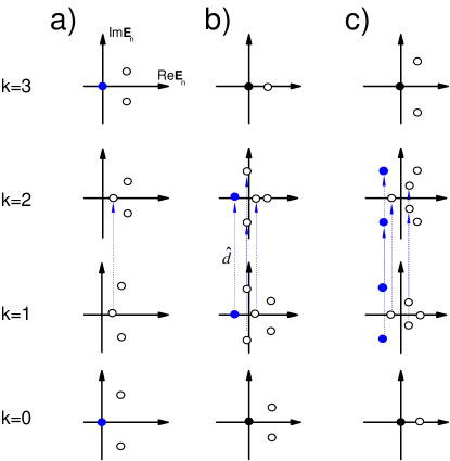
Figure 1: (color online) The three possible spectra of the stochastic evolution operator of the STS of a model with the phase space being a three-dimentional compact sphere. Such models have only two supersymmetric eigenstates (big dots at the origin) in one-to-one correspondence with the two De Rahm cohomology classes of the 3D sphere in the zeroth (k=0) and the third (k=3) degree. Spectrum (a) corresponds to the unbroken topological supersymmetry because both ground states are supersymmetric with one of them (for $k=3$) being the state of thermodynamic equilibrium. The other two spectra (b and c) correspond to the “chaotic” dynamics, i.e., to the situations when the ground states (big leftmost dots) are non-supersymmetric because they have non-zero eigenvalues. The eigenstates of the stochastic evolution operator that represent the modes of the magnetic field in the KD theory are the non-$\hat{d}$-symmetric pairs of 1- and 2-forms connected by the dashed lines representing the action of the d-operator. Note that the SEO spectra for 1- and 2-forms may also have other eigenstates (with positive real parts of their eigenvalues) that can not be associated with the magnetic field. Those from $\Omega^{0}$ can be though of as the eigenstates of the gauge potential $\varphi\in\Omega^{0}$ with which one can perform the gauge-invariance transformation of the vector potential, $A\to A+\hat{d}\varphi$, without changing the magnetic field. The additional non-$\hat{d}$-closed eigenmodes in $\Omega^{2}$ are unphysical because they correspond to the magnetic field configurations such that $\hat{d}F=\left(\mathrm{div}B\right)d^{3}x\neq 0$, i.e., they contain magnetic monopoles.

The supersymmetric structure of the SEO separates all eigenstates into two groups:

• Almost all eigenstates come in non-supersymmetric “bosonic-fermionic” pairs, $|\alpha\rangle$ and $|\alpha^{\prime}\rangle=\hat{d}|\alpha\rangle$, that have the same eigenvalue because $\hat{H}$ commutes with $\hat{d}$.

• Some of the eigenstates are the supersymmetric singlets $|\theta\rangle$ that are non-trivial in the De Rahm cohomology. Supersymmetry of a state $|\theta\rangle$ means that it is $\hat{d}$-closed, $\hat{d}|\theta\rangle=0$, but not $\hat{d}$-exact, meaning that no $\theta^{\prime}$ exists such that $|\theta\rangle=\hat{d}|\theta^{\prime}$$\rangle$.

The $\hat{d}$-exact form of the SEO, i.e., $\hat{H}=[\hat{d},\hat{\bar{d}}]$, implies that all eigenstates with non-zero eigenvalue are non-supersymmetric. Indeed, for $\hat{H}|\alpha\rangle=\mathcal{E_{\alpha}}|\alpha\rangle$ and $\mathcal{E_{\alpha}}\neq 0$ we have two possibilities:

1. The first possibility is that $\hat{d}|\alpha\rangle\neq 0$. In this case the statement is trivial because $\hat{H}$ commutes with $\hat{d}$ and consequently the state $|\alpha^{\prime}\rangle=\hat{d}|\alpha\rangle\neq 0$ has the same eigenvalue, $\hat{H}|\alpha^{\prime}\rangle=\mathcal{E_{\alpha}}|\alpha^{\prime}\rangle$, and we have a non-supersymmetric “boson-fermion” pair, $|\alpha\rangle$ and $|\alpha^{\prime}\rangle$.

2. The other possibility is that $\hat{d}|\alpha\rangle=0$. Then, using $\hat{H}=\hat{\bar{d}}\hat{d}+\hat{d}\hat{\bar{d}}$ and the fact that $\hat{d}|\alpha\rangle=0$ we have $\mathcal{E}_{\alpha}|\alpha\rangle=(\hat{\bar{d}}\hat{d}+\hat{d}\hat{\bar{d}})|\alpha\rangle=\hat{d}\hat{\bar{d}}|\alpha\rangle$, thus $|\alpha\rangle=\hat{d}|\tilde{\alpha}\rangle,$ with $|\tilde{\alpha}\rangle=\hat{\bar{d}}|\alpha\rangle/\mathcal{E}_{\alpha}$. Up to a “gauge”, i.e., up to a $\hat{d}$-closed piece, $|\tilde{\alpha}\rangle=|\tilde{\alpha}^{\prime}\rangle+|\tilde{\alpha}^{\prime\prime}\rangle$ with $\hat{d}|\tilde{\alpha}^{\prime\prime}\rangle=0$ is an eigenstate of the SEO with the same eigenvalue as $|\alpha\rangle$. Again, we have a boson-fermion pair of eigenstates $|\alpha\rangle=\hat{d}|\tilde{\alpha}^{\prime}\rangle\in\Omega^{k}$ and $|\tilde{\alpha}^{\prime}\rangle\in\Omega^{k-1}$ of the same eigenvalue.

In this manner, all eigenstates with non-zero eigenvalues are non-$\hat{d}$-symmetric boson-fermion pairs of states. Thus we just came to an important conclusion – all supersymmetric singlet states have vanishing eigenvalues.

This implies that any growing mode of a KD cannot be a supersymmetric state of the corresponding SEO. Operational KDs must exhibit a broken supersymmetry.

III.3 Non-magnetic modes

Let us now investigate whether the dynamo phenomenon must be intrinsic to magnetic fields, or whether other quantities described by 0- or 3-forms could be amplified exponentially by the Lie action of a stationary flow field.

Any physically meaningful stochastic model must have the steady-state (zero-eigenvalue) total probability distribution, $\psi_{\mathrm{TE}}=P_{\mathrm{TE}}d^{3}x\in\Omega^{3}\>$ with $\int_{x}\psi_{\mathrm{TE}}=1.$ This state can be recognized as the state of thermodynamic equilibrium (TE). This eigenstate is supersymmetric because $\hat{d}\psi_{\mathrm{TE}}=0$, which is true for all 3-forms, and it is not $\hat{d}$-exact because otherwise its integral over $X$ would vanish. This state is always the “ground state” for $\Omega^{3}$. In other words, among all the eigenstates in $\Omega^{3}$, the state of thermodynamic equilibrium has the least real part of its eigenvalue and this is zero. This can be seen from the following qualitative, yet robust argument.

All non-$\hat{d}$-symmetric eigenstates $\alpha$ from $\Omega^{3}$ are $\hat{d}$-exact, i.e., of the form $|\alpha\rangle=\hat{d}|\alpha^{\prime}\rangle$.. The integral of the kets of these states is zero, $\int_{X}\alpha=\int_{X}\hat{d}\alpha^{\prime}=0$, which means that their wavefunctions must be negative at least somewhere on $X$.

Imagine now that the “ground state” on $\Omega^{3}$ is a non-$\hat{d}$-symmetric eigenstate with a real negative eigenvalue. An arbitrary total probability distribution will have non-zero contribution from such an eigenstate. Its temporal evolution according to Eq. (28) will lead to a state dominated by this eigenstate after sufficiently long time of evolution as this state is an exponentially growing mode. Consequently, the total probability distribution will become negative somewhere on the phase space, since this state must be negative in some regions of the phase space as discussed in the previous paragraph.

A negative probability distribution is of course illogical and therefore in contradiction to the above assumption that a non-$\hat{d}$-symmetric state with negative eigenvalue exists in $\Omega^{3}$. Using similar reasoning one can also rule out the possibility of a pair of Ruelle-Pollicott resonances with a negative real part of their eigenvalues being the ground states on $\Omega^{3}$. Thus, one arrives at the conclusion that the supersymmetric state of thermodynamic equilibrium is always the “ground state” of $\Omega^{3}$. It can be said that the conventional Focker-Planck operator $\hat{H}^{(3)}$ never breaks supersymmetry spontaneously, i.e., its ground state is always supersymmetric.

This means that density modes do not grow infinitely under a stationary flow, but saturate in this supersymmetric state.

It can also be shown that $\hat{H}^{(0)}$ is related by a similarity transformation to $\hat{H}_{\mathrm{T}}^{(3)}$, where $\hat{H}_{\mathrm{T}}$ is the SEO of the time-reversed SDE, i.e., the SDE with the opposite flow vector field and the above argumentation also applies to $\hat{H}_{\mathrm{T}}^{(3)}$. Operators related by a similarity transformation are isospectral so that $\hat{H}^{(0)}$ must also never break the supersymmetry on its own, just as $\hat{H}^{(3)}$. In conclusion, in three dimensions, only non-supersymmetric 1-forms and 2-forms can spontaneously break the overall supersymmetry of the SEO. For this reason, a dynamo mechanism is only known for the vector potential of the magnetic fields, but not for the scalar potential of the electric field.

The above discussion leads to the conclusion that there are only three possible forms of spectra of SEO (see Fig. 1), with the 1- and 2-forms being the eigenstates of the KD operator. The first type in Fig. 1a corresponds to the unbroken topological supersymmetry because the ground states of the model are supersymmetric. The other two types of spectra correspond to the spontaneously broken topological supersymmetry because the ground states have non-zero eigenvalues and therefore are non-supersymmetric. These correspond to growing KD modes, either just exponentially growing, or with a superimposed oscillation.

III.4 Stochastic chaos

It is known that non-diffusive KDs require some non-integrability of the underlying flow, which is a signature of (deterministic) chaos (Ott, 2007).The centerpiece of the theory of deterministic chaos is the butterfly effect (BE), which is a high sensitivity of the subsequent evolution of a system to perturbations and/or variations in initial conditions. The BE is often regarded as the defining property of chaos (Motter, 2014; Ruelle, 2014). The supersymmetry breaking picture of stochastic chaos provides a theoretical explanation of the BE via the Goldstone theorem (Ovchinnikov, 2014).

In order to identify spontaneous topological supersymmetry breaking with the emergence of deterministic chaos we investigate the number of periodic trajectories of a dynamical systems. It is well-known that in many deterministic chaotic systems, the number of periodic trajectories grows exponentially as a function of their periods in the long-time limit. This exponential growth comes from the infinite number of unstable periodic orbits with unlimited periods that constitute strange or chaotic attractors (Gilmore, 1998). In Ref. (Ovchinnikov, 2014), it was shown that for some classes of models the stochastically averaged number of periodic solutions must be represented by the dynamical partition function,

$$Z_{t}|_{t\to\infty}=\mathrm{Tr}\,e^{-t\hat{H}}|_{t\to\infty}\approx$$

$$\approx\sum_{g}e^{-t\mathcal{E}_{g}}=\begin{cases}\begin{array}[]{cc}\mathrm{const}&\mbox{Fig. 1a,}\\ 2\,e^{t\,|\mathcal{E}_{g}|}&\mbox{Fig. 1b,}\\ 4\,\cos(t\,\mathrm{Im}\mathcal{E}_{g})\,e^{t\,|\mathrm{Re}\mathcal{E}_{g}|}&\mbox{Fig. 1c,}\end{array}\end{cases}.$$

where the label $g$ runs over the ground states. This equation shows that for spectra as displayed in Fig. 1b, the stochastically averaged number of periodic solutions must grow exponentially. The broken topological supersymmetry therefore seems to be a prerequisite for deterministic chaos in deterministic as well as in stochastic systems. Therefore, this spectral classification of dynamical chaos seems to be the natural generalization of the concept of deterministic chaos to the stochastic regime.

In the case of a spectrum as displayed in Fig. 1c, the dynamical partition function can become negative. This implies that in this case the dynamical partition function cannot represent the stochastically averaged number of periodic solutions. Furthermore, there are theorems in the dynamical system theory stating that for a certain class of (expanding) models that mimic chaotic behavior, the eigenvalue of the ground state must be real. In the light of these theorems, the spectrum in Fig. 1c looks suspicious.

This raises the question whether such STS spectra are realizable. Here, the KD-STS correspondence proves useful for the STS. As flow configurations which exhibit growing oscillating KD modes are known (Baryshnikova and Shukurov, 1987; Ruzmaikin et al., 1988; Li et al., 2010b) the existence of spectra like shown in Fig. 1c are realizable.

III.5 The limit of the KD-STS correspondence

The reported KD-STS correspondence is in a sense accidental. It is possible due to the linearity of the induction equation and its specific form, i.e., the Lie derivative along the velocity field representing the evolution of magnetic field lines frozen into the media. In a more general situation as given by the nonlinear dynamo, this picture breaks down. On the other hand, the STS is applicable to all stochastic and deterministic differential equations and the dynamical equations of the non-linear dynamo is one of them. If the STS theory of the nonlinear dynamo would be constructed, it would be a full-fledged “field theory” with an infinite-dimensional phase space of magnetic field configurations as compared to the finite-dimensional phase space of test particle trajectories considered here for the KD. Instead of Eq. (27), the underlying equation of motion will be the induction equation itself. The magnetic field (and perhaps other functions/fields over the real space) would no longer be the “wavefunction”, as in case of the KD, but rather the coordinates of the model, whereas the wavefunctions would depend on them in a functional manner.

IV Conclusion

We established a correspondence between the theory of KD and the recently found approximation-free STS. We showed that the KD equation is essentially the stochastic evolution operator of a related SDE and thus it possesses topological supersymmetry. This connection allowed us to identify the KD effect as the supersymmetry breaking phenomenon in the corresponding SDE. We further argued that the SDEs related to KDs with growing magnetic modes are chaotic in a generalized stochastic sense. We showed that the flow pattern of stationary KDs can only amplify quantities associated with vector potentials (like magnetic fields) but not those associated with scalar potentials or which are densities.

Furthermore, the existence of the growing modes of the magnetic field in the KDs can be viewed as a proof that the supersymmetry breaking spectra of the stochastic evolution operator with both real and complex conjugate eigenvalues of the ground states are realizable. This finding is valuable for the STS. We believe that further work may reveal other important insights on both sides of the KD-STS correspondence established in this paper.

V Acknowledgements

This work was supported partly by the Excellence Cluster Universe. I.V.O. would like to thank the Max Planck Institute for Astrophysics for the hospitality during his visit in the summer 2015. T.A.E. thanks the International Space Science Institute (ISSI) in Bern for its hospitality and the ISSI International Team 323 for a stimulating atmosphere. We acknowledge valuable comments on the manuscript by David Butler, Sebastian Dorn, Maksim Greiner, Reimar Leike, Daniel Pumpe and Theo Steininger.

References

- Bullard and Gellman (1954) E. Bullard and H. Gellman, Royal Society of London Philosophical Transactions Series A 247, 213 (1954).
- Parker (1955) E. N. Parker, ApJ 122, 293 (1955).
- Braginskiy (1964) S. I. Braginskiy, Geomagnetism and Aeronomy 4, 572 (1964).
- Parker (1970) E. N. Parker, ApJ 162, 665 (1970).
- Krause and Raedler (1980) F. Krause and K.-H. Raedler, Organic Photonics and Photovoltaics (1980).
- RÃŒdiger (2004) R. RÃŒdiger, G. Hollerbach, The Magnetic Universe: Geophysical and Astrophysical Dynamo Theory (Wiley-VCH Verlag GmbH & Co, KGaA, 2004).
- Parker (1992) E. N. Parker, ApJ 401, 137 (1992).
- Beck et al. (1994) R. Beck, A. D. Poezd, A. Shukurov, and D. D. Sokoloff, A&A 289, 94 (1994).
- Subramanian (1998) K. Subramanian, MNRAS 294, 718 (1998), astro-ph/9707280 .
- Beck (2007) R. Beck, A&A 470, 539 (2007), arXiv:0705.4163 .
- Ruzmaikin et al. (1989) A. Ruzmaikin, D. Sokolov, and A. Shukurov, MNRAS 241, 1 (1989).
- Dolag et al. (2002) K. Dolag, M. Bartelmann, and H. Lesch, A&A 387, 383 (2002).
- Enßlin and Vogt (2006) T. A. Enßlin and C. Vogt, A&A 453, 447 (2006), astro-ph/0505517 .
- Vazza et al. (2014) F. Vazza, M. Brüggen, C. Gheller, and P. Wang, MNRAS 445, 3706 (2014), arXiv:1409.2640 .
- Parker (1975) E. N. Parker, ApJ 198, 205 (1975).
- Glatzmaier (1984) G. A. Glatzmaier, Journal of Computational Physics 55, 461 (1984).
- Raedler (1986) K.-H. Raedler, Astronomische Nachrichten 307, 89 (1986).
- Charbonneau and MacGregor (2001) P. Charbonneau and K. B. MacGregor, ApJ 559, 1094 (2001).
- Spruit (2002) H. C. Spruit, A&A 381, 923 (2002), astro-ph/0108207 .
- Braithwaite (2006) J. Braithwaite, A&A 449, 451 (2006), astro-ph/0509693 .
- Browning (2008) M. K. Browning, ApJ 676, 1262 (2008), arXiv:0712.1603 .
- Taylor (1963) J. B. Taylor, Royal Society of London Proceedings Series A 274, 274 (1963).
- Kuang and Bloxham (1997) W. Kuang and J. Bloxham, Nature 389, 371 (1997).
- Lerche (1971) I. Lerche, ApJ 166, 627 (1971).
- Roberts (1972) P. H. Roberts, Royal Society of London Philosophical Transactions Series A 272, 663 (1972).
- Li et al. (2010a) K. Li, P. W. Livermore, and A. Jackson, Journal of Computational Physics 229, 8666 (2010a).
- Motter (2014) D. K. Motter, Adilson E. Campbell, Physics Today 66, 27 (2014).
- Ott (2007) E. Ott, Chaos, Kinetics and Nonlinear Dynamics in Fluids and Plasmas 511, 263 (2007).
- Ovchinnikov (2013) I. V. Ovchinnikov, Chaos: An Interdisciplinary Journal of Nonlinear Science 23, 013108 (2013).
- Ovchinnikov (2014) I. V. Ovchinnikov, arXiv:1308.4222 (2014).
- Baryshnikova and Shukurov (1987) I. Baryshnikova and A. Shukurov, Astronomische Nachrichten 308, 89 (1987).
- Ruzmaikin et al. (1988) A. Ruzmaikin, D. Sokolov, and A. Shukurov, Journal of Fluid Mechanics 197, 39 (1988).
- Li et al. (2010b) K. Li, P. W. Livermore, and A. Jackson, J. Comput. Phys. 229, 8666 (2010b).
- Dutta and Horn (1981) P. Dutta and P. M. Horn, Rev. Mod. Phys. 53, 497 (1981).
- Aschwanden (2011) M. Aschwanden, Self-Organized Criticallity in Astrophysics: Statistics of Nonlinear Processes in the Universe (Springer-Verlag, Berlin, Heidelberg, 2011).
- Gutenberg and Richter (1955) B. Gutenberg and C. F. Richter, Nature 176, 795 (1955).
- Beggs and Plenz (2003) J. M. Beggs and D. Plenz, The Journal of Neuroscience 23, 11167 (2003).
- Witten (1982) E. Witten, Journal of Differential Geometry 17, 661 (1982).
- Frenkel et al. (2007) E. Frenkel, A. Losev, and N. Nekrasov, Nuclear Physics B - Proceedings Supplements 171, 215 (2007), the proceedings of the International Conference on Strings and Branes: The present paradigm for gauge interactions and cosmology (Cargèse School on String Theory) Cargèse 2006.
- Labastida (1989) J. M. F. Labastida, Communications in Mathematical Physics 123, 641 (1989).
- Witten (1988a) E. Witten, Communications in Mathematical Physics 118, 411 (1988a).
- Witten (1988b) E. Witten, Communications in Mathematical Physics 117, 353 (1988b).
- Birmingham et al. (1991) D. Birmingham, M. Blau, M. Rakowski, and G. Thompson, Physics Reports 209, 129 (1991).
- Mostafazadeh (2002) A. Mostafazadeh, Nuclear Physics B 640, 419 (2002).
- Ruelle (2014) D. Ruelle, Physics Today 67, 9 (2014).
- Manning (2006) A. Manning, in Dynamical Systems, Lecture Notes in Mathematics, Vol. 468 (Springer, 2006) p. 185.
- Gilmore (1998) R. Gilmore, Rev. Mod. Phys. 70, 1455 (1998).
- Ruelle (2002) D. Ruelle, Notices of AMS 49, 887 (2002).