Hydrodynamic Interactions between Two Forced Objects of Arbitrary Shape: II Relative Translation

Abstract

We study the relative translation of two arbitrarily shaped objects, caused by their hydrodynamic interaction as they are forced through a viscous fluid in the limit of zero Reynolds number. It is well known that in the case of two rigid spheres in an unbounded fluid, the hydrodynamic interaction does not produce relative translation. More generally such an effective pair-interaction vanishes in configurations with spatial inversion symmetry; for example, an enantiomorphic pair in mirror image positions has no relative translation. We show that the breaking of inversion symmetry by boundaries of the system accounts for the interactions between two spheres in confined geometries, as observed in experiments. The same general principle also provides new predictions for interactions in other object configurations near obstacles. We examine the time-dependent relative translation of two self-aligning objects, extending the numerical analysis of our preceding publication [Goldfriend, Diamant and Witten, Phys. Fluids 27, 123303 (2015)]. The interplay between the orientational interaction and the translational one, in most cases, leads over time to repulsion between the two objects. The repulsion is qualitatively different for self-aligning objects compared to the more symmetric case of uniform prolate spheroids. The separation between the two objects increases with time $t$ as $t^{1/3}$ in the former case, and more strongly, as $t$, in the latter.

I Introduction

Hydrodynamic interactions are crucial for the dynamics of colloidal dispersions Happel and Brenner (1983); Russel et al. (1989). These flow-mediated interactions are characterized by a long-ranged $R^{-1}$ decay with distance $R$. The effect of hydrodynamic interactions is particularly strong in the case of driven systems, where an external force acts on each constituent object. This effect is apparent already at the level of a single object, where the combination of driving and hydrodynamics generally leads to rotation-translation coupling Happel and Brenner (1983). At the level of a forced pair of objects the hydrodynamic interaction gives rise to rich behavior, as presented in the preceding article Goldfriend et al. (2015) (referred to hereafter as Publication I) and the present one. On the collective level of driven suspensions, the long-ranged and strong hydrodynamic interactions may create large-scale dynamical structures, as in colloid sedimentation Ramaswamy (2001).

The hydrodynamic interaction between two forced symmetric objects, e.g., spheres, has been explored extensively in the middle of the last century; see Ref. Happel and Brenner (1983) and references therein. In the limit of zero Reynolds number, the hydrodynamic interaction between two identical sedimenting spheres, isolated in an unbounded fluid, does not bring about any relative translation, i.e., the spheres neither reduce nor increase their mutual distance while settling through the fluid (they do not rotate around each other either). This remarkable result can be related to the time-reversal symmetry of the Stokes equations governing the flow field Ramaswamy (2001).

On the other hand, the vanishing relative velocity in the case of two spheres is readily violated by changing the system’s geometry. For example, Squires and Brenner Squires and Brenner (2000) pointed out that, when forced away from a nearby wall, two spheres do develop relative velocity, making them approach one another. Such long-ranged attraction between two like-charged spheres in the presence of a similarly charged wall was observed in optical tweezers experiments by Larsen and Grier Larsen and Grier (1997). These apparent interactions do not originate from any direct, e.g., electrostatic or van der Waals interaction, but from the velocity fields generated by the objects (and sometimes are referred to as “hydrodynamic pseudo-potentials” Squires (2001)). Another example of an attraction-like behavior, mediated by Stokes flow, appears in the motion of two spheres driven along an optical vortex trap Sokolov et al. (2011). The effects of such interactions can show up in experiments not only as pair-attractions but also in more complex phenomena, such as collective phonon-like excitations in driven object arrays Nagar and Roichman (2014); Beatus et al. (2012).

These previous studies of apparent interactions originating in hydrodynamic coupling were ad hoc, treating specific experimental scenarios. In this article we address two more general questions: (i) At zero Reynolds number, what are the geometrical configurations for which relative translation between two objects necessarily vanishes? (ii) In cases where it does not vanish, what are the consequences for the long-time trajectories of the two objects? Looking for properties of general applicability, we consider arbitrarily shaped objects and do not restrict ourselves to a specific geometry. Symmetry considerations have been successfully invoked in the past for various hydrodynamic problems at zero Reynolds number, e.g., the motion of objects in shear flow Bretherton (1962); Makino and Doi (2005), or Purcell’s theorem for swimmers Purcell (1977). Similarly, we seek general laws, derivable from symmetry arguments, concerning the relative translation of driven object pairs.

In the inertia-less regime the flow and the velocities of suspended objects at a given moment are proportional to the external forces acting at that moment. Consequently, the motion of two interacting objects can be expressed by a grand pair-mobility matrix Brenner (1964a); Brenner and O’Neill (1972); Kim and Karrila (2005); Goldfriend et al. (2015). Earlier works focused on the mobility (or inversely, hydrodynamic resistance) of objects in various simple geometries, such as a pair of spheres or spheroids Goldman et al. (1966); Wakiya (1965); Felderhof (1977); Jeffrey and Onishi (1984); Liao and Krueger (1980); Kim (1985, 1986). In addition, several numerical techniques were developed to study dispersions of arbitrarily shaped colloids Karrila et al. (1989); Tran-Cong and Phan-Thien (1989); Carrasco and de la Torre (1999); Kutteh (2010); Cichocki et al. (1994). In Publication I, we have studied general properties of the hydrodynamic interaction and considered its effect on orientational dynamics. In the present article, we extend this study, focusing on translational motion of object pairs.

The motivation of Publication I was to understand the role of hydrodynamic interactions between self-aligning objects . An object is self-aligning if, when subjected to an external unidirectional force (as in sedimentation), it achieves terminal alignment between a specific eigen-direction affixed to the object and the force direction, owing to a translation–rotation coupling in its mobility Krapf et al. (2009); Moths and Witten (2013a, b). (See also Sec.III.1 below.) We focused on self-aligning objects of irregular shape, which have a richer response as they also rotate with a constant angular velocity about the aligning direction. To this end, we explored the pair-mobility of two identical, arbitrarily shaped objects, which are arranged in the same orientation. Based on general considerations, and utilizing the system’s symmetry under exchange of objects, we proved that self-aligning objects undergo relative rotation, as well as relative translation, when forced through an unbounded fluid. The leading effective interaction is dipolar, scaling as $R^{-2}$ with the mutual distance $R$ between the objects. In addition, we used a numerical integration scheme to study the effect of these pair-interactions over time. We found that the majority of our examples, comprising pairs of randomly constructed, self-aligning stokeslet objects, showed a repulsive-like behavior, where the objects move away from each other in time.

These two key results, concerning the instantaneous and long-times interactions, have led to the present work, which extends the analysis along two separate directions: (a) In Sec. II we continue to study the instantaneous response of object pairs, i.e., the rigorous properties of the pair-mobility matrix. We provide examples for configurations with spatial inversion symmetry, where the relative translation vanishes, as well as simple geometries, for which this symmetry is broken. (b) In Sec. III we return to examine in more detail the repulsive trend in the far-field time evolution of self-aligning object pairs, providing a quantitative explanation of the phenomenon. We further compare it to the time evolution of two non-alignable objects (uniform prolate spheroids), and point out the qualitative difference between the two cases. Finally, the implications of our results, from theoretical and experimental points of view, are discussed in Sec IV.

II Instantaneous Response

II.1 Pair Mobility Matrix

We consider a system of two rigid objects, $a$ and $b$, with typical size $l$, subject to external forces and torques $\vec{F}^{a}$, $\vec{F}^{b}$ and $\vec{\tau}^{a}$, $\vec{\tau}^{b}$ in a fluid of viscosity $\eta$. The geometry of the system, i.e., the shape of each of the objects and the fluid boundaries, are arbitrary. Each of the objects is designated with an origin about which its linear velocity and torque are measured. In the regime of zero Reynolds number (also known as Stokes flow, creeping flow or inertia-less flow), the objects respond with instantaneous linear and angular velocities through a symmetric, positive-definite $12\times 12$ pair-mobility matrix Happel and Brenner (1983); Brenner and O’Neill (1972); Goldfriend et al. (2015),

$$\begin{pmatrix}\vec{V}^{a}\\ \vec{\omega}^{a}l\\ \vec{V}^{b}\\ \vec{\omega}^{b}l\end{pmatrix}=\frac{1}{\eta l}\begin{pmatrix}\mathbb{A}^{aa}&(\mathbb{T}^{aa})^{T}&\mathbb{A}^{ab}&(\mathbb{T}^{ba})^{T}\\ \mathbb{T}^{aa}&\mathbb{S}^{aa}&\mathbb{T}^{ab}&\mathbb{S}^{ab}\\ (\mathbb{A}^{ab})^{T}&(\mathbb{T}^{ab})^{T}&\mathbb{A}^{bb}&(\mathbb{T}^{bb})^{T}\\ \mathbb{T}^{ba}&(\mathbb{S}^{ab})^{T}&\mathbb{T}^{bb}&\mathbb{S}^{bb}\end{pmatrix}\begin{pmatrix}\vec{F}^{a}\\ \vec{\tau}^{a}/l\\ \vec{F}^{b}\\ \vec{\tau}^{b}/l\end{pmatrix}.$$ (1)

The dimensionless blocks of the matrix defined in Eq. (1) depend on the whole geometry of the system (the shapes of the objects, their mutual configuration, as well as the shapes of the surrounding boundaries), the boundary conditions at all the surfaces, and the choice of objects’ origins. The transformation between matrices which differ in the choice of objects’ origins can be found in Appendix A of Publication I. Hereafter we normalize the viscosity such that $\eta l=1$.

In this work we focus on the translational dynamics of two forced objects (without external torques), which is given by a $6\times 6$ sub-matrix of the pair-mobility, indicated hereafter by $\mathbb{A}$,

$$\begin{pmatrix}\vec{V}^{a}\\ \vec{V}^{b}\end{pmatrix}=\begin{pmatrix}\mathbb{A}^{aa}&\mathbb{A}^{ab}\\ \mathbb{A}^{ba}&\mathbb{A}^{bb}\end{pmatrix}\begin{pmatrix}\vec{F}^{a}\\ \vec{F}^{b}\end{pmatrix}.$$ (2)

The diagonal blocks, $\mathbb{A}^{aa}$ and $\mathbb{A}^{bb}$, correspond to the response of an object to a force on itself, in the presence of the other object. The off-diagonal blocks, $\mathbb{A}^{ab}$ and $\mathbb{A}^{ba}$, correspond to the hydrodynamic interaction, i.e., the response of one object to a force on the other. The properties of the full pair-mobility matrix in Eq. (1) imply that $\mathbb{A}$ is positive definite and symmetric Condiff and Dahler (1966); Happel and Brenner (1983); Landau and Lifshitz (1980). The matrix $\mathbb{A}$ has additional symmetries, as discussed in the next section.

II.2 Symmetrical Pair Configurations

Brenner Brenner (1964a) (see also Ref. Happel and Brenner (1983), Sec. 5.5) characterized the properties of the self-mobility matrix for individual, symmetric objects. Given a symmetry of the object’s shape, he deduced which of the hydrodynamic responses vanish. For example, if an object has a plane of reflection symmetry, forcing it in the direction perpendicular to that plane cannot lead to translation parallel to the plane. For instance, forcing a spheroid along its major axis does not induce translation along its two other principal axes.

As a first step, we consider the transformation of the pair-mobility matrix under various operations— spatial proper and improper rotations (rotations combined with reflections), and exchange of objects. We note that the positions of the objects’ origins, i.e., the external forcing points, are an essential part of the system geometry. In this section we will restrict our treatment to cases where the forcing point is at the geometric centroid of the object, that is, the center of mass if the object has a uniform mass density. Consider the transformation between two pair-mobility matrices which differ by a rigid rotation. Given the rotation matrix $\mathbb{R}$ between a given configuration and the rotated one, the blocks in $\mathbb{A}$, being all tensors, transform accordingly: $\mathbb{A}^{aa}\rightarrow\mathbb{R}\mathbb{A}^{aa}\mathbb{R}^{T}$, $\mathbb{A}^{ab}\rightarrow\mathbb{R}\mathbb{A}^{ab}\mathbb{R}^{T}$ and $\mathbb{A}^{bb}\rightarrow\mathbb{R}\mathbb{A}^{bb}\mathbb{R}^{T}$. The same law applies to the transformation between systems which differ by a rigid improper rotation with improper rotation matrix $\bar{\mathbb{R}}$. We note here that the twist matrices $\mathbb{T}$, the blocks in Eq. (1) which relate forces to angular velocities, are pseudo-tensors; thus, their transformation under improper rotation includes a change of sign, $\mathbb{T}^{aa}\rightarrow-\bar{\mathbb{R}}\mathbb{T}^{aa}\bar{\mathbb{R}}^{T}$. Since the pair-mobility matrix inherently refers to two distinguishable objects, $a$ and $b$, we should also consider its transformation under interchanging the objects’ labeling, $a\leftrightarrow b$. This transformation corresponds to interchanging the blocks $\mathbb{A}^{aa}\leftrightarrow\mathbb{A}^{bb}$ and $\mathbb{A}^{ab}\leftrightarrow\mathbb{A}^{ba}$; or, in matrix form,

$$\mathbb{A}\rightarrow\mathbb{E}\mathbb{A}\mathbb{E}^{-1},$$ (3)

where $\mathbb{E}$ is a $6\times 6$ matrix which interchanges the objects,

$$\mathbb{E}=\begin{pmatrix}0&\mathbb{I}_{3\times 3}\\ \mathbb{I}_{3\times 3}&0\end{pmatrix},$$ (4)

and $\mathbb{I}_{3\times 3}$ is the $3\times 3$ identity matrix.

As mentioned in Sec. I, at zero Reynolds number, sedimentation of two identical rigid spheres in an unbounded fluid does not induce relative motion of the two spheres. In contrast, we showed in Publication I that two identical, arbitrarily shaped objects in an unbounded fluid, under the same forcing, may attract or repel each other. In addition, using the symmetry of such a system under exchange of objects, we found the leading (dipolar) order of this effective interaction at large mutual separation. We now examine the hydrodynamic interaction for several symmetric configurations. In this part of the article we focus on what symmetry has to tell us, and do not yet anticipate when its consequences are useful. To demonstrate the resulting principles, therefore, we allow ourselves to examine specially designed configurations. Examples for the usefulness of these principles will be given later on.

II.2.1 Two Enantiomers in an Unbounded Fluid

As the first example, we examine a system possessing inversion symmetry. The spatial inversion of the Stokes equations under reversing time has been shown to imply fundamental consequences concerning the dynamics of rigid objects. For example, it was used previously to deduce generic properties of shear flow response, in the cases of a single spheroid Bretherton (1962) and an enantiomeric non-interacting pair Makino and Doi (2005). The fact that the instantaneous response, under the same forcing, of pair-configurations with spatial inversion symmetry does not induce relative translation may have already been given elsewhere; yet, we are not aware of works which give a rigorous derivation of it. Accordingly, we review this basic result below from matrix transformations and time-reversibility points of view.

Consider a system of two enantiomers in an unbounded fluid as depicted in the left panel of Fig. 1. We choose the mutual orientation of the objects such that one object is the mirror image of the other; hence, the system’s geometry is invariant under spatial inversion, $\vec{r}\to-\vec{r}$. This symmetry implies that the pair-mobility matrix is invariant under two consecutive operations (see Fig. 1): spatial inversion followed by exchange of objects’ labels, or, in matrix form, $\mathbb{A}=\mathbb{E}(-\mathbb{I}_{6\times 6})\mathbb{A}(-\mathbb{I}_{6\times 6})\mathbb{E}^{-1}$, where $\mathbb{E}$ has been defined in Eq. (4). This last equality yields $\mathbb{A}^{aa}=\mathbb{A}^{bb}=\mathbb{A}^{\text{self}}$ and $\mathbb{A}^{ab}=\mathbb{A}^{ba}=\mathbb{A}^{\text{coupling}}$, i.e.,

$$\text{Enantiomeric pair:}\ \ \ \mathbb{A}=\begin{pmatrix}\mathbb{A}^{\text{self}}&\mathbb{A}^{\text{coupling}}\\ \mathbb{A}^{\text{coupling}}&\mathbb{A}^{\text{self}}\end{pmatrix},$$ (5)

which applies in fact for any inversion-symmetric situation. This form of the pair-mobility matrix implies that, under the same force $\vec{F}$, the two objects will develop identical velocities, $\vec{V}^{a}=\vec{V}^{b}=(\mathbb{A}^{\text{self}}+\mathbb{A}^{\text{coupling}})\cdot\vec{F}$. Thus: the instantaneous response under the same forcing of a pair, whose configuration possesses an inversion symmetry, does not include relative translation. As noted above, a system of two sedimenting spheres is a particular example of this general result.

The vanishing relative motion in a system which is invariant under spatial inversion can be understood alternatively by the following argument. Assume by negation that two enantiomers in an unbounded fluid develop a relative velocity under the same forcing. Without loss of generality, let us take the case when the two objects get closer together; see configuration (a) in the right panel of Fig. 1. The mirror configuration of the system ($\vec{r}\to-\vec{r}$), depicted in configuration (b), implies that the two also get closer when reversing the forces. On the other hand, Stokes equations are invariant under inversion of time and forces; hence, reversing the forces in configuration (a) should make the objects get further apart, as depicted in configuration (c). Since (b) and (c) represent the same system, we reach a contradiction, and deduce that the relative velocity between the two enantiomers must vanish.

To summarize, it is inversion symmetry that governs the vanishing relative velocity between two forced objects at zero Reynolds number; hence, whenever this symmetry is broken one should expect relative translation.

An important remark bears mentioning here. The instantaneous rotational response of the enantiomeric pair corresponds to two opposite rotations, i.e., non-vanishing relative angular velocity. (See Publication I.) With time, the opposite rotations will break the inversion symmetry, unless there are additional symmetries, for example, when the objects’ shapes are isotropic, as in the case of two spheres. While the example of two enantiomers whose mutual symmetry is only instantaneous may seem artificial, the principle that it demonstrates is useful. Driving forces will sometimes bring bodies close to a symmetric situation, and then one will find especially simple motions that call for explanation. In particular, two irregular objects can be aligned by the driving Krapf et al. (2009); Moths and Witten (2013a, b) and then we should be interested in the question of whether they keep their distance or drift apart. Moreover, not only a pair of spheres will preserve inversion symmetry over time. Another example is two ellipsoids, or indeed a pair of any bodies of revolution with fore-aft symmetry, whose axes are aligned on a plane perpendicular to the force; see Fig. 2(a). Without any calculation, we can assert that such two objects will maintain their relative position over time. The additional symmetry of the system imposes relative rotation only about the axes of symmetry ($y$-axis in Fig. 2(a)), which does not break the inversion symmetry. Another example will be given in the Discussion.

                 

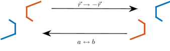
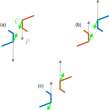
Figure 1: Schematic description of the arguments presented in Sec. II.2.1 for the vanishing instantaneous relative motion between two forced enantiomers. The left panel describes how the mirror symmetry of the system is expressed in terms of spatial inversion combined with interchanging the objects. The right panel demonstrates the arguments based on the symmetry of the Stokes equations under inversion of time and forces, where gray (thin) and green (thick) arrows indicate forces and velocities respectively. Configuration (b) is the spatial inversion of configuration (a) whereas configuration (c) is the response of configuration (a) under the opposite forcing.

II.2.2 Configurations with One Reflection Plane and Exchange Symmetry

We now turn to examples where the symmetry is broken by the confining boundaries. The first system consists of two spheres, placed on a plane parallel to a wall; see Fig 2(b). This system was used in Ref. Squires and Brenner (2000) to interpret the attraction between two like-charged spheres near a similarly charged wall, as was observed in optical-tweezers experiments Larsen and Grier (1997). The geometry of the system is invariant under two successive operations: reflection about the symmetry plane of the two spheres and interchanging the objects. We denote by $\parallel$ and $\perp$ the directions parallel and perpendicular, respectively, to the mirror plane, i.e., perpendicular and parallel, respectively, to the wall itself. The reflection leaves vectors parallel to the mirror plane unchanged but reverses vectors normal to that plane. Using the transformation laws introduced above, we find that the blocks of $\mathbb{A}$, which relate forces perpendicular to the wall and objects’ velocities parallel to the wall, must satisfy $\mathbb{A}^{aa}_{\perp\parallel}=-\mathbb{A}^{bb}_{\perp\parallel}$ and $\mathbb{A}^{ab}_{\perp\parallel}=-\mathbb{A}^{ba}_{\perp\parallel}$. These restrictions imply that, under forcing toward or away from the wall (e.g., as the spheres are electrostatically repelled from the wall Larsen and Grier (1997)), the objects respond in opposite directions in the plane parallel to the wall, $\vec{V}^{a}_{\perp}=(\mathbb{A}^{aa}_{\perp\parallel}+\mathbb{A}^{ab}_{\perp\parallel})F_{\parallel}=-\vec{V}^{b}_{\perp}$. Note that the symmetry of the system alone does not tell us whether the objects repel or attract under a given forcing direction. The analysis in Ref. Squires and Brenner (2000) showed that forcing away from the wall results in an apparent attraction between the pair, in agreement with the experiment. It should be stressed that, unlike specific calculations as in Ref. Squires and Brenner (2000), our symmetry principle is neither restricted to spheres, nor to the limit of small objects, nor to the limit of large separations.

The complete form of the pair-mobility matrix as a result of the geometrical restrictions in this system is given in Appendix B, Eq. (15), along with the explicit expressions for point objects. Another interesting conclusion, arising solely from the system’s symmetry, is that, since $\mathbb{A}^{aa}_{\perp\parallel}=-\mathbb{A}^{bb}_{\perp\parallel}$ and $\mathbb{A}^{ab}_{\perp\parallel}=-\mathbb{A}^{ba}_{\perp\parallel}$, forcing the spheres parallel to the wall will result in one sphere approaching the wall and the other moving away from it.

As a second example, let us consider the system addressed in Ref. Sokolov et al. (2011) — two spheres forced to move along a ring; see Fig. 2(c). The corresponding pair-mobility matrix can be written in polar coordinates $(\rho,\theta)$. The system is invariant under two successive operations: inversion of the $\theta$ coordinate, $\theta\to-\theta$, and interchanging the objects. Hence, this system is similar to the previous one in the sense that it is symmetric under objects exchange by inversion of one coordinate. This leads to $\mathbb{A}^{aa}_{\rho\theta}=-\mathbb{A}^{bb}_{\rho\theta}$ and $\mathbb{A}^{ab}_{\rho\theta}=-\mathbb{A}^{ba}_{\rho\theta}$. Consequently, under the same forcing along the tangential direction, the spheres respond with opposite velocities along the radial direction. Sokolov et al. used a holographic optical vortex trap to study this system and observed the radial symmetry breaking experimentally Sokolov et al. (2011). In addition, they found that this effect, combined with a confining radial potential, results in overall attraction along the ring as the system evolves in time. Once again, the symmetry argument derived here is far more general than the specific limit studied theoretically in Ref. Sokolov et al. (2011).

We note that the results obtained above, regarding configurations with one reflection plane of symmetry, should also be derivable using time-reversal arguments, as was done in the case of an enantiomeric pair.

     

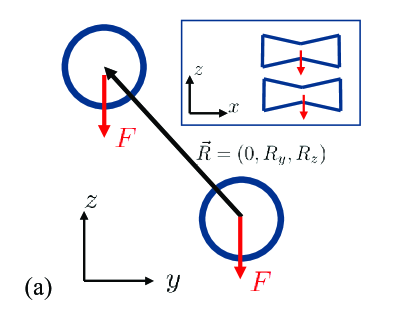
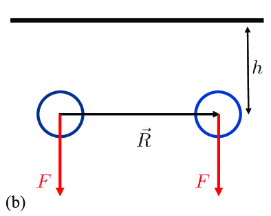
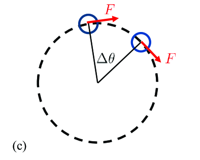
Figure 2: The three systems discussed in Secs. II.2.1 and II.2.2: (a) Two identical axisymmetric objects, with fore-aft symmetry, where the vector connecting their origins is perpendicular to their symmetry axes. (b) A pair of spheres near a wall. The spatial separation between the spheres is represented by the vector $\vec{R}$ which connects their origins. (c) A pair of spheres driven along a ring. The angular separation is indicated by $\Delta\theta$.

III Far-Field Dynamics of two Forced Objects in Unbounded Fluid

In the preceding section we considered the instantaneous response of a pair of objects given the symmetries of their configuration. The analysis of this linear problem, derived from symmetry arguments, is useful to determine the stability of a given state of the system. However, it might be inapplicable to the time-dependent trajectories, since a configuration symmetry at a given time can be broken by subsequent motion. A well known example is the sedimentation in an unbounded fluid of two prolate spheroids, which start with their major axes parallel to the force Wakiya (1965); Kim (1985); Kutteh (2010). The initial inversion symmetry about the plane perpendicular to the force, which, according to the discussion in Sec. II, precludes any relative translation, soon breaks due to the rotation of each spheroid, and relative velocity appears (see a more detailed analysis below). In general, since the instantaneous response depends on configuration, the time-dependent trajectories of a driven pair is a non-linear, multi-variable problem. We are compelled, therefore, to implement numerical integration for specific examples, and try to identify general trends. In this section we consider the time evolution of two objects under the same constant driving. In particular, we provide further insight into the results reported in Publication I concerning the combined effects of rotational and translational interactions.

III.1 Dynamics of an isolated object

Before describing the time evolution of object pairs, it is essential to introduce the different types of objects that we consider hereafter and describe their dynamics, under a unidirectional force, at the single-object level. For more details on the various orientational behaviors of single objects, see Refs. Krapf et al. (2009); Gonzalez et al. (2004). In the absence of external torque, the linear and angular velocities of an object are given, respectively, by $\mathbb{A}_{0}\cdot\vec{F}$ and $\mathbb{T}_{0}\cdot\vec{F}$, where $\mathbb{A}_{0}$ and $\mathbb{T}_{0}$ are $3\times 3$ blocks of the object’s self-mobility matrix. These blocks depend on the shape of the object, its orientation, and the position of the forcing point.

We consider three types of objects: (a) Uniform prolate spheroid — a spheroid whose forcing point is located at its geometric centroid, as in the case of spheroids with a uniform mass density. For such an object $\mathbb{T}_{0}=0$; hence, it does not rotate, regardless of its orientation. The translation direction of a uniform spheroid is in the plane spanned by its major axis and the forcing direction Happel and Brenner (1983). (b) Self-aligning prolate spheroid — a prolate spheroid whose forcing point is displaced from the centroid along its major principal axis, e.g., spheroids with a non-uniform mass density. These objects have an antisymmetric $\mathbb{T}_{0}$ matrix. For any initial orientation, a self-aligning spheroid rotates toward a state where its major axis, and therefore its translation direction, is aligned with the external force. We use type (b) as a simple example, which can be treated analytically, for self-aligning objects. (c) Self-aligning object of irregular shape — an object whose $\mathbb{T}_{0}$ matrix has only one real, non-zero eigenvalue. These objects reach an ultimate alignment between a specific eigen-direction affixed to the object (the eigenvector corresponding to the real eigenvalue) and the force, together with a uniform right- or left-handed rotation about it (according to the sign of the real eigenvalue) Krapf et al. (2009); Moths and Witten (2013a, b). As in Publication I we use the particularly simple construction of stokeslet objects — a discrete set of small spheres, separated by much larger, rigid distances, where each sphere is approximated by a point force. Constructing them randomly, we avoid objects of pre-designed shapes.

III.2 Far-Field Equations

Let us assume that there are no external torques on the objects, such that we can choose their origins as their forcing points. We consider the case in which the objects are subjected to the same forcing $\vec{F}$. The mutual separation between the objects $a$ and $b$ is designated with the vector $\vec{R}$, whose direction is defined from the origin of $a$ to the origin of $b$. While time-integrating the equations it is essential to take into account the coupling between translation and rotation. Thus, we must work with the complete pair-mobility matrix, Eq. (1), which gives

$$\dot{\vec{R}}=\vec{V}^{a}-\vec{V}^{b} = \left(\mathbb{A}^{aa}+\mathbb{A}^{ab}-\mathbb{A}^{bb}-\mathbb{A}^{ba}\right)\cdot\vec{F}$$ (6)

$$\vec{\omega}^{a} = \left(\mathbb{T}^{aa}+\mathbb{T}^{ab}\right)\cdot\vec{F}$$ (7)

$$\vec{\omega}^{b} = \left(\mathbb{T}^{bb}+\mathbb{T}^{ba}\right)\cdot\vec{F}.$$ (8)

A major simplification, from both the analytical and the numerical points of view, is to consider pairs with separation much larger than the typical size of the individual object $l$, and study the corresponding far-field interaction. In Publication I we studied a system of two arbitrarily shaped objects in an unbounded fluid, and derived the general form of the pair-mobility matrix up to second order in $l/R$. The zeroth-order term corresponds to two non-interacting objects; The first-order term accounts for the advection of one object by the Oseen flow generated by the other, which results in a common translation of the pair with velocity $\mathbb{G}(\vec{R})\cdot\vec{F}\sim R^{-1}$ and with no relative translation; The second order term, $\sim\vec{\nabla}\mathbb{G}\sim R^{-2}$, is the leading term which can give rise to relative translation between the objects via hydrodynamic interactions.

The equations governing the objects’ mutual separation and their rotations read

$$\dot{\vec{R}} = \left[(\mathbb{A}_{0}^{a}-\mathbb{A}_{0}^{b})+(\Pi^{a}+\Pi^{b}):\vec{\nabla}\mathbb{G}(\vec{R})-\vec{\nabla}\mathbb{G}(\vec{R})^{T}:(\Pi^{a}+\Pi^{b})^{T}\right]\cdot\vec{F}$$ (9)

$$\vec{\omega}^{a} = \left[\mathbb{T}_{0}^{a}+(\Psi^{a}-\frac{1}{2}\mathcal{E}):\vec{\nabla}\mathbb{G}(\vec{R})\right]\cdot\vec{F}$$ (10)

$$\vec{\omega}^{b} = \left[\mathbb{T}_{0}^{b}-(\Psi^{b}-\frac{1}{2}\mathcal{E}):\vec{\nabla}\mathbb{G}(\vec{R})\right]\cdot\vec{F},$$ (11)

where $\mathbb{A}_{0}$, $\mathbb{T}_{0}$ and $\Pi$, $\Psi$ are single-object-dependent tensors of rank 2 and 3, respectively, which depend on the individual object’s shape and orientation, and $\mathcal{E}$ is the Levi-Civita tensor. In Publication I we introduced a tensor $\Phi$ with dimensions $6\times 3\times 3$; here we separate it into its translational part, $\Pi$, and rotational part, $\Psi-\frac{1}{2}\mathcal{E}$, each with dimensions $3\times 3\times 3$. The tensors $\mathbb{A}_{0}$ and $\mathbb{T}_{0}$ are the zeroth order blocks (the blocks in the self-mobility matrices), which give the linear and angular velocities of a single object when it is subjected to external force. The tensors $\Pi$ and $\Psi$ correspond to the linear- and angular-velocity responses to a flow gradient at the object’s origin. When these tensors are coupled with $\vec{\nabla}\mathbb{G}$ they construct second-order terms of the pair-mobility matrix, describing the direct hydrodynamic interaction between the objects. The term which is proportional to $\mathcal{E}$ is also a part of the second-order term, giving the rotation of one object with the vorticity generated by forcing the other. The tensors $\mathbb{A}_{0}$, $\mathbb{T}_{0}$ and $\Pi$ depend on the choice of objects’ origins; for the corresponding transformations see Appendices A and B in Publication I, or Ref. Kim and Karrila (2005).

III.3 Transversal Repulsion under Constant Forcing

In Publication I we examined the effect of hydrodynamic interactions on the orientational evolution of two identical, self-aligning objects. Using numerical integration we followed the time-dependent trajectories of pairs of stokeslet objects under two types of driving— a constant force and a rotating one. The latter, in the absence of hydrodynamic interactions, tends to synchronize each object with the rotating force Moths and Witten (2013a, b). We noticed that in most (though not all) of the studied examples the two identical, self-aligning objects effectively repelled each other when subjected to the same driving (see solid red curve in Fig. 4(a)). (Counter-examples, such as limit-cycle trajectories, were observed as well.) The increasing separation is transversal— taking place within the plane perpendicular to the average force direction. Below we explain the nature of this repulsion, focusing on the simpler case of constant forcing.

III.3.1 Two self-aligning objects

Let us consider the time evolution of the following system, depicted in Fig. 3: two identical self-aligning spheroids, positioned initially along the $x$-axis, and subjected to a constant force along the $(-\hat{z})$ direction. Self-aligning spheroids are achieved by separating the center of forcing from their centroids, e.g., through a nonuniform mass density under gravity. The configuration has an inversion symmetry about the $yz$-plane. It does not have an inversion symmetry about the $xy$-plane unless the spheroids are aligned along $\hat{z}$. Thus, according to Sec. II, unless aligned, they are expected to have an instantaneous relative velocity. We denote by $\theta$ the angle between the force and the major axis of each spheroid; $l$ indicates the length of the major axis, and $h$ is the displacement of the forcing point from the centroid. For given $h$ and $\theta$, the individual-object’s tensors which appear in Eqs. (9)–(11) can be found from the known tensors for $h=0$ and $\theta=0$ (e.g. Ref. Happel and Brenner (1983)) by a change of origin and rotation transformation. According to Sec. III.1, in the absence of interactions and $\theta\neq 0$, two uniform prolate spheroids will maintain their relative tilt and glide away from each other with a constant velocity, whereas two self-aligning ones will do the same but with velocity decreasing in time as they get aligned with the force. In order to examine the effect of hydrodynamic interactions we take the initial condition $\theta(t=0)=0$, for which relative translation vanishes in their absence. Using the calculated individual-object’s tensors for self-aligning spheroids, the equations of motion for the pair in the far-field regime $R\gg l$ and $\theta\ll 1$, Eqs. (9)–(11), are then reduced to the following simple form (recall that we set $\eta l=1$):

$$\dot{R} = \left[\alpha\theta+\zeta\left(\frac{l}{R}\right)^{2}\right]\frac{F}{8\pi}$$ (12)

$$l\dot{\theta} = \left[-\lambda\theta+\left(\frac{l}{R}\right)^{2}\right]\frac{F}{8\pi},$$ (13)

where the dimensionless parameters $\alpha$, $\zeta$ and $\lambda$ (derivable from the single-object tensors) depend on the spheroid’s aspect ratio and $h/l$. (More details on the derivation of the above equations are given in Appendix C.) Using the conventions of Fig. 3, $\alpha>0$ and $\lambda\geq 0$; hence, positive $\theta$ implies increasing separation and decreasing tilt. Differentiating Eq. (12), and substituting $\dot{\theta}$ from Eq. (13), we obtain the equation for the separation alone,

$$\ddot{x}=-(\lambda+2\zeta x^{-3})\frac{F}{8\pi l}\dot{x}+(\alpha+\lambda\zeta)x^{-2}\left(\frac{F}{8\pi l}\right)^{2},$$ (14)

where we have set $x\equiv R/l$.

The translational dynamics is dictated by (i ) opposite mutual glide of one object away from the other, and (ii ) direct hydrodynamic interaction which decays as $R^{-2}$. (We neglect the higher-order correction of the interaction $\sim\theta R^{-2}$.) The evolution of the tilt angle $\theta$ is governed by two competitive effects— the vorticity which increases it and the tendency of the individual spheroid to align with the force. The fact that the effect of direct hydrodynamic interaction on the angular velocities is independent of the object’s shape is specific to configurations in which $\vec{R}\perp\vec{F}$, regardless the object’s geometry . The effect of additional separation along the force direction is discussed at the end of this section.

The dotted blue curves in Fig. 4 show an example of a numerical solution of Eqs. (12)–(13). Initially $\theta$ increases linearly due to the vorticity term in Eq. (13). After a typical time of $\sim(\lambda F/8\pi l)^{-1}$ this increase is suppressed by the alignability of each object, and at $t\to\infty$, the separation increases as $t^{1/3}$ while $\theta$ decreases to 0 according to a $t^{-2/3}$ law. These asymptotic laws can easily be inferred analytically. The growth in mutual separation is a combination of a gliding term ($\alpha$) and an interaction term ($\zeta>0$). We note, however, that the $t^{1/3}$ law arises from the alignability alone, whereas the direct interaction can only quantitatively affect the dynamics. As seen from Eq. (14) in the limit of large $x$, the equivalent system in classical mechanics is the damped equation $\ddot{x}=-B\dot{x}+Ax^{-2}$. At long times, $t\gg B^{-1}$, acceleration is negligible and we are left with the equation $\dot{x}=(A/B)x^{-2}$ for the velocity. This equation yields the terminal $x\sim t^{1/3}$ law of the dotted blue curve in Fig. 4(a).

Next, we consider the repulsive time-dependent trajectories in the more general case of two self-aligning objects of irregular shape. We emphasize that this general case is expected to show a richer behavior; this has been illustrated in Publication I for stokeslets objects, where, for example, attractive-like behavior was observed as well. The repulsive trend reported in Publication I occurs in the majority ($\sim 80\%$) of our several dozens examples comprising randomly constructed 4-stokeslets objects. In addition, in the far-field limit, it is independent of the initial separation along the force direction, as well as the initial mutual orientation. Here, we illustrate how the theoretical result derived for self-aligning spheroids is evident also in the effective repulsion between two self-aligning objects of arbitrary shape.

Self-aligning objects of irregular shape exhibit complex dynamics already on the single-object level, as they acquire ultimate rotation about their eigen-direction. For example, their terminal translation direction is not necessarily constant and might rotate about the forcing direction. Here we consider two identical arbitrarily shaped objects, in which the pair configuration has no spatial symmetry. The coordinate space includes the mutual separation $\vec{R}$ and the orientation variables of each object, where we represent the latter with Euler-Rodriguez 4-parameters (or unit quaternions) Goldfriend et al. (2015); Favro (1960); Kutteh (2010). The resulting equation of motion for this coordinate space is a set of coupled non-linear, first-order ODEs, which can be solved with conventional techniques; see Appendix C for details of the integration scheme. The objects are initially separated along the $x$-axis and aligned with the force (which, as before, is along the negative $z$-axis). These specific initial conditions are used to emphasize the comparison with the pair of spheroids. As opposed to the spheroid pair, where the eigen-directions rotate only about the $y$-axis and the separation unit-vector $\hat{R}$ is fixed to its initial direction $\hat{x}$, here the former and the latter undergo a complex, 3D rotational motion.

We follow the dynamics of each object’s eigen-direction, which is affixed to the object-reference-frame and denoted by $-\hat{Z}$. For each object we define a tilt angle $\cos\theta(t)\equiv\ \hat{Z}(t)\cdot\hat{z}$, and an azimuthal correlation with the separation vector $\cos\phi(t)\equiv\ -\hat{Z}_{\perp}(t)\cdot\hat{R}_{\perp}(t)$. A scheme of the configuration with the relevant variables is depicted in Fig. 3. The two objects can effectively glide away from each other, in resemblance to the case of two self-aligning spheroids, if the eigen-directions are tilted away from the separation direction, that is, $\cos\phi^{\,a}(t)=1$ and $\cos\phi^{b}(t)=-1$; see inset in the right panel of Fig. 3. The solid red curves in Fig. 4, which correspond to a representative example, consisting of two identical objects, demonstrate that such resemblance between the two cases does exist. In particular, the solid red curve in Fig. 4(b) shows that $\theta(t)$ of object $a$ follows the same trend as the dotted blue curve which represents the simple example of self-aligning spheroids. The tilt angle of object $b$, which is not shown, has a similar behavior. The inset in Fig. 4(a) shows the opposite correlations between $\hat{Z}^{a}$, $\hat{Z}^{b}$ and $\vec{R}$. The gliding effect results in an effective repulsion, $R(t)\propto t^{1/3}$, as can be seen in Fig. 4a. The direct interaction term in Eq. (9)— proportional to $\Pi$ and decaying as $R^{-2}$— can also contribute to the $t^{1/3}$ trend.

The example of an arbitrarily shaped, self-aligning pair, presented in Fig. 4, is a representative of a half-dozen other examples not shown here. These randomly generated examples correspond to initial conditions, which involve also longitudinal separation and different mutual orientations. The variance in the measured exponents is within a small numerical error, of order 5%. The analytically predicted power law was found to hold for all pairs of objects which drifted far apart in the simulations (80% of the examples). This implies that the $1/3$ exponent for the asymptotic repulsion is most probably general for the class of self-aligning objects.

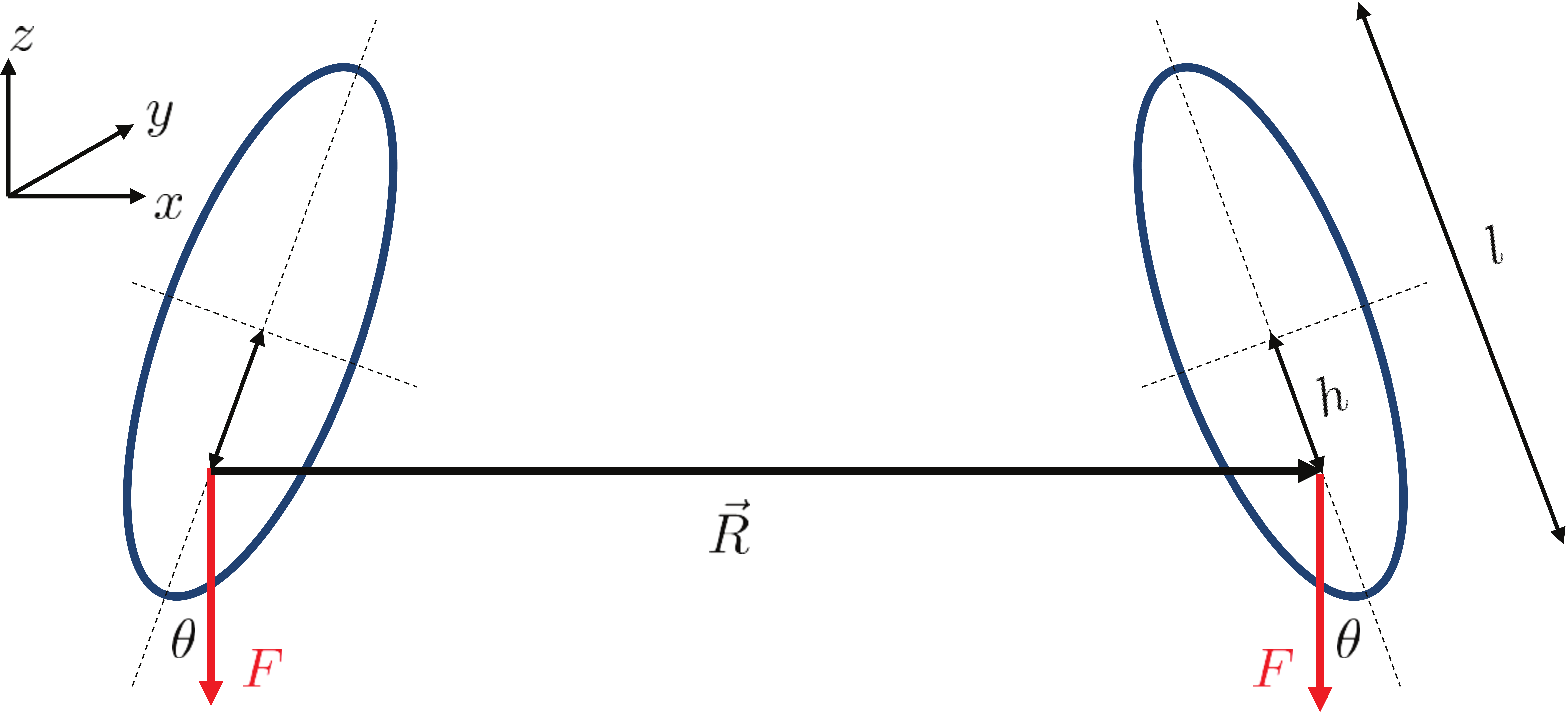
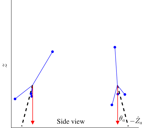
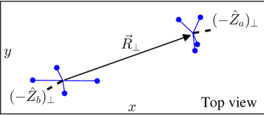
Figure 3: Left panel: system of two self-aligning, prolate spheroids. The tilt angle $\theta$ is between the force and the major axis of the object, and $h$ indicates the shifted position of the forcing point. Right panel: system of two identical self-aligning objects made of 4 stokeslets. In the absence of interaction the eigen-direction of each object $(-\hat{Z})$ would eventually align with the force which is along the $(-\hat{z})$ axis (not drawn), and rotate about it with constant angular velocity. The hydrodynamic interaction tilts the objects by angles $\theta_{a}$ and $\theta_{b}$, while keeping a correlation between the transversal direction of the eigen-directions and the separation vector. This effect results in repulsion between the objects while they continuously rotate in the $xy-$plane. Here we show a snapshot of this terminal evolution. The main figure shows the projection of the system (the objects and their eigen-directions) onto the $xz$-plane, whereas the inset shows the $xy-$plane projection, together with the separation vector $\vec{R}$.

                 

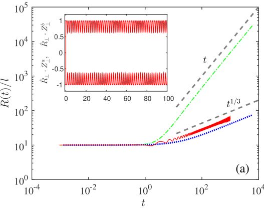
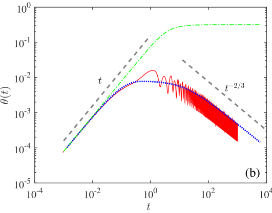
Figure 4: Representative trajectories for systems of two uniform spheroids (dash-dotted green curves), a pair of self-aligning spheroids (dotted blue curves), and two self-aligning stokeslets objects (solid red curves), together with the asymptotic behaviors at short and long times (gray dashed lines). The results are presented in dimensionless units by setting the parameters of length and time to $l=1$ and $(\lambda F/8\pi l)^{-1}=0.1$, and the additional parameters to the values detailed in Appendix C. The distance between the objects is shown in panel (a), exhibiting the effective repulsion between the two objects. The inset demonstrates the correlation between the eigen-directions and the separation vector in the case of self-aligning irregular objects. Panel (b) shows the evolution of the tilt angle (the solid red curve corresponds to only one of the objects).

III.3.2 Two uniform prolate spheroids

A pair of uniform spheroids exhibits quite different behavior from that of two self-aligning objects. An individual uniform spheroid ($h=0$) does not rotate under forcing, and does not translate in response to a flow gradient, i.e., the $\mathbb{T}_{0}$ matrices and $\Pi$ tensors in Eqs. (9)–(11) vanish . Hence, in the far field dynamics of two uniform spheroids the alignability and direct interaction are absent, i.e., $\lambda=\zeta=0$ in Eqs. (12) and (13). The resulting picture, arising from Eqs. (12) and (13), is that $\theta$ increases linearly with time until saturating to a constant value, which depends on $R(t=0)$, and the objects move away from each other with a constant terminal velocity ; see also dash-dotted green curves in Fig. 4. Hence, the role of hydrodynamic interactions in this case is solely the generation of opposite tilts between the objects, which, as a result, move in opposite directions. In this case, Eq. (14) becomes equivalent to the one-dimensional problem from classical mechanics of two particles with a central repulsive potential, $\ddot{x}=Ax^{-2}$, and the initial conditions $x(0)=x_{0}$ and $\dot{x}(0)=0$. The qualitative behavior is apparent from the corresponding velocity equation $\dot{x}=\sqrt{2A(x^{-1}_{0}-x^{-1})}$. The positive velocity increases $x$, which in turn increases $\dot{x}$ toward a constant value, whereby $x$ continues to grow linearly with time.

The two power laws — $R(t)\sim t^{1/3}$, derived theoretically for self-aligning spheroids and demonstrated numerically for irregular objects, and $R(t)\sim t$, derived in the symmetric case of two uniform spheroids — are universal. Thus, the repulsive dynamics of pairs of symmetric objects and self-aligning objects are superficially similar, in that both arise from opposite tilts of the two objects. However, the mechanisms of the two repulsions differ qualitatively. The additional tendency of the latter objects to align with the force leads to a decrease in the relative velocity, as reflected by a weaker power law for the increase of separation with time. In addition, the terminal relative velocity in the case of two uniform spheroids is sensitive to the initial separation, as well as to the initial tilts. By contrast, the self-aligning pair has a stable asymptotic velocity independent of the initial state of alignment (assuming that $R(t=0)\gg l$ such that the far-field equations, Eqs. (9)–(11), are valid).

III.3.3 Effect of longitudinal separation

Up until now we have examined the simple case of constant force with initial separation perpendicular to its direction. As explained below, a small additional separation along the direction of the force should not alter qualitatively the transversal repulsion.

The evolution of the longitudinal separation differs from the transversal one. The two components governing the far-field transversal dynamics — mutual relative orientation between the objects (the opposite tilt) and the direct interaction which decays as $R^{-2}$ — are weaker, or even absent, in the longitudinal dynamics. First, the direct interaction, originating from the off-diagonal blocks of the pair-mobility $\mathbb{A}$, vanishes due to the constraint that $\mathbb{A}$ is a symmetric matrix Condiff and Dahler (1966); Happel and Brenner (1983); Landau and Lifshitz (1980). The components relating one object’s linear velocity along the $\hat{z}$ direction with forcing on the other, satisfy $\mathbb{A}^{ab}_{zz}=\mathbb{A}^{ba}_{zz}$, which implies $\dot{R}_{z}=(\mathbb{A}^{ab}_{zz}-\mathbb{A}^{ba}_{zz})(-F)=0$. Hence, relative longitudinal dynamics is solely dictated by relative orientation between the objects, which in the far-field regime corresponds to the difference between the (unperturbed) self-responses of each object.

When $R_{z}\ll R_{\perp}$ we can approximate the objects’ orientations by two opposite tilts of their eigen-directions. If the object’s shape is invariant under rotations about the eigen-direction, e.g., self-aligning spheroid, such relative orientation cannot yield relative velocity along the $z$-axis. In the case of arbitrarily shaped, self-aligning objects, we expect that any asymmetry about the eigen-direction approximately averages out by the rotation of each object. Thus, the effect of opposite tilts on the relative translation along the direction of the force is weaker than that on the transversal one. Indeed, the examples in Publication I showed that the longitudinal separation evolves slowly in time and seems to saturate at long times.

IV Discussion

This work, together with Publication I, aims to provide a comprehensive description of the translational and orientational hydrodynamic interactions between two forced objects, focusing on the generic features of these interactions. In particular, we have derived a formalism to predict from the system’s symmetry whether the hydrodynamic interactions create relative motion (orientational or translational) between the objects. Where relative motion is present, we have analyzed its multipole expansion. While our symmetry-based results for the instantaneous interaction are rigorous, we could provide only qualitative general trends concerning the time-dependent relative motion, focusing particularly on irregular, self-aligning objects, and on the asymptotic dynamics at long times.

The present, second article has been devoted to the relative motion between two equally forced objects. The first part (Sec. II) has established the basic geometry dependence of the effective interaction. We have proven that invariance under spatial inversion precludes any instantaneous relative translation. In the second part (Sec. III), we have treated the effect of hydrodynamic interactions on time-dependent trajectories. We have demonstrated how the characteristic $R_{\perp}(t)\sim t^{1/3}$ repulsion between two self-aligning objects differs qualitatively from the counterpart, asymptotic $R_{\perp}(t)\sim t$ behavior, which corresponds to two uniform spheroids. The preferred alignment of the individual objects reduces the relative tilt as they get further apart, thus decreasing their relative translation compared to the constantly tilted spheroids. This case highlights the sharp contrast between motion conditioned by current configuration and time-integrated motion. Two initially aligned spheroids do not have instantaneous relative velocity, while two self-aligning objects do (due to the direct interaction, $\sim R^{-2}$, term). Yet, the orientational interaction between the spheroids makes them oppositely tilt and achieve with time an asymptotic translational velocity which exceeds that of the self-aligning objects.

We have applied our general symmetry criterion to systems with confining boundaries, which break inversion symmetry. This geometrical consideration, without any further detail, accounts for the apparent interactions originated in hydrodynamic coupling, which were observed in optical-tweezers experiments involving two confined configurations Larsen and Grier (1997); Sokolov et al. (2011). Previous works Squires and Brenner (2000); Sokolov et al. (2011) examined these apparent interactions for two point-like objects. Our treatment shows that the existence of the effect can be inferred by symmetry. It is present, therefore, in more general situations, such as non-spherical objects (e.g., Fig 2(a)) and arbitrary separations, including objects in close proximity.

The general theory presented here can be used to obtain simple qualitative predictions, which are readily testable in experiment. A particularly simple example is the sedimentation of two identical spheres, positioned one above the other parallel to a vertical planar wall. This configuration will result in one sphere instantaneously approaching the wall, while the other being repelled from the wall. Another example is a modification of the experiment presented in Ref. Sokolov et al. (2011). Two identical spheres placed in a ring and forced in the radial direction will develop relative translation in the tangential direction. We note that the general symmetry criterion concerns only the existence or absence of interaction. To determine the sign of the interaction, whether it is repulsive or attractive, one needs additional information such as the Green’s function of the given hydrodynamic problem.

The symmetry arguments, which we have applied in the first part of the paper, can be found useful in the examination of orientational dynamics. In a system with spatial inversion symmetry, object $a$ has the same translational response as object $b$, and an opposite rotational response. Hence, when the objects are subjected to opposite forces, e.g., in the presence of a central force of interaction between them, they must rotate in the same sense, and spatial inversion symmetry will be maintained at all times. This means that, in the dynamics of an enantiomorphic pair under opposite drive, relative orientations, possessing a spatial inversion symmetry, are fixed points in the orientational space, preserving a constant phase difference. The study of this effect and its applications is postponed to a future publication.

Another result, which can be verified in a simple experimental setup, is the asymptotic power-law time dependence of the separation between two self-aligning objects. For the particular system comprising a pair of self-aligning (non-uniform) prolate spheroids we have shown analytically a $t^{1/3}$ trend (Sec. III). In the case of two, arbitrarily shaped self-aligning objects, where repulsion is not a general law (see Publication I), we have reported several examples with a similar trend. These examples, which are represented by the red curve in Fig. 4, are not sensitive to initial conditions. For spheroids, the effect of opposite tilts on the mutual repulsion is captured by the positive glide parameter $\alpha$ in Eq. (12). The sign of $\alpha$ is dictated by the elongated shape of the individual spheroid. (An oblate spheroid has a negative $\alpha$.). Therefore, good candidates for arbitrarily shaped, repulsive pairs may be elongated objects, whose properties, when averaged over rotations about the eigen-direction, resemble those of self-aligning spheroids. A suggestion for an experiment includes tracking the sedimentation of two micron-sized, self-aligning objects in a viscous fluid, where optical traps can be used to place the objects at a fixed initial separation, perpendicular to gravity. The effect should not depend on the initial orientations of the objects, as their alignability guarantees that after a short transient they will be close to their aligned state.

Finally, the distinction between irregular objects and regular ones, on the level of a pair of objects, should be significant, in particular, in driven suspensions with many-body interactions. Traditionally, theories and simulations of fluidized beds focused on colloidal objects of spherical or rod-like shape (see reviews in Refs. Ramaswamy (2001) and Guazzelli and Hinch (2011) and references therein); however, the case of self-aligning irregular objects might give rise to new phenomena. For example, sedimentation of spheres involves only three-body effective interactions, whereas a suspension of sedimenting irregular objects will include effective pair-interactions. Such pair interactions should affect the objects’ velocity correlations, as will be addressed in a future publication.

Appendix A Notation

The dynamics of arbitrarily shaped objects is complex and involves mathematical structures of various dimensions. In order to facilitate the readability of the formalism, we use the following notation regarding vectors, tensors, and matrices:

1. 3-vectors are denoted by an arrow, $\vec{v}$, and unit 3-vectors by a hat, $\hat{v}$.

2. Matrices are marked by a blackboard-bold letter, e.g., $\mathbb{M}$, where the dimension of the matrix is understood from the context.

3. Tensors of rank 3 are denoted by a capital Greek letter, e.g., $\Phi$.

4. $\mathbb{I}_{n\times n}$ is the $n\times n$ identity matrix.

5. Tensor multiplication — the dot notation, $\cdot$ — denotes a contraction over one index. The double dot notation, $:$, denotes a contraction over two indices. Thus, given a tensor $\Upsilon$ of rank $N$ and a tensor $\Xi$ of rank $M>N$, the tensors $\Upsilon\cdot\Xi$ and $\Upsilon:\Xi$ are tensors of rank $N+M-2$ and $N+M-4$. For example, for $\Upsilon$ of rank 2 and $\Xi$ of rank 3, $(\Xi\cdot\Upsilon)_{ikj}=\Upsilon_{is}\,\Xi_{skj}$ and $(\Upsilon:\Xi)_{j}=\Upsilon_{ks}\,\Xi_{skj}$.

6. The matrix $\vec{Y}^{\times}$ obtained from the vector $\vec{Y}$ is defined as $(\vec{Y}^{\times})_{ij}=\epsilon_{ikj}Y_{k}$, such that, for any vector $\vec{X}$, $\vec{Y}^{\times}\cdot\vec{X}=\vec{Y}\times\vec{X}$.

Appendix B Pair-Mobility Matrix of Two Spheres Near a Wall

Here we provide more details regarding the pair-mobility matrix of a system comprising two spheres near a wall. We write down the blocks structure of the corresponding $\mathbb{A}$ and provide an explicit expressions for the case of point-like objects. A schematic description of the system is given in Fig. 2b. Without loss of generality we assume that the spheres are located along the $x$-axis, where $\vec{R}=x\hat{x}$ points from the origin of sphere $a$ to the origin of sphere $b$, and the wall is placed parallel to them at height $z=h$. The spheres’ radii are denoted by $\rho$. Hereafter we consider the projection of $\mathbb{A}$ onto the $xz$-plane. The properties of the $y$-axis components can be deduced from the additional symmetry of reflection about the $xz$-plane, which was not included in our analysis above. According to the discussion in Sec. II.2.2 the pair-mobility matrix of this system has the following form:

$$\mathbb{A}=\begin{pmatrix}A^{\text{self}}_{xx}&A^{\text{self}}_{xz}&A^{\text{coupling}}_{xx}&A^{\text{coupling}}_{xz}\\ A^{\text{self}}_{zx}&A^{\text{self}}_{zz}&A^{\text{coupling}}_{zx}&A^{\text{coupling}}_{zz}\\ A^{\text{coupling}}_{xx}&-A^{\text{coupling}}_{xz}&A^{\text{self}}_{xx}&-A^{\text{self}}_{xz}\\ -A^{\text{coupling}}_{zx}&A^{\text{coupling}}_{zz}&-A^{\text{self}}_{zx}&A^{\text{self}}_{zz}\end{pmatrix}.$$ (15)

The number of independent components can be reduced further by using the fact that $\mathbb{A}$ is symmetric. This property is not related to the system geometry, which is the issue of Sec. II.2.2, but rather results from Onsager relations or conservation of angular momentum in the system Condiff and Dahler (1966); Happel and Brenner (1983); Landau and Lifshitz (1980). The symmetry of $\mathbb{A}$ connects between the $xz$ and $zx$ components: $A^{\text{self}}_{xz}=A^{\text{self}}_{zx}$ and $A^{\text{coupling}}_{xz}=-A^{\text{coupling}}_{zx}$. Finally, we get

$$\mathbb{A}=\begin{pmatrix}A^{\text{self}}_{xx}&A^{\text{self}}_{xz}&A^{\text{coupling}}_{xx}&A^{\text{coupling}}_{xz}\\ A^{\text{self}}_{xz}&A^{\text{self}}_{zz}&-A^{\text{coupling}}_{xz}&A^{\text{coupling}}_{zz}\\ A^{\text{coupling}}_{xx}&-A^{\text{coupling}}_{xz}&A^{\text{self}}_{xx}&-A^{\text{self}}_{xz}\\ A^{\text{coupling}}_{xz}&A^{\text{coupling}}_{zz}&-A^{\text{self}}_{xz}&A^{\text{self}}_{zz}\end{pmatrix}.$$ (16)

In the case of point-like objects, i.e., spheres with infinitely small radius, the blocks can be calculated explicitly. The self blocks are given by the self-mobility of a single sphere near a plane wall (first-order in $\rho/h$) Happel and Brenner (1983)

$$\mathbb{A}^{\text{self}}=\frac{1}{6\pi\eta\rho}\begin{pmatrix}1-\frac{9}{16}\frac{\rho}{h}&0\\ 0&1-\frac{9}{8}\frac{\rho}{h}\end{pmatrix}.$$

The coupling blocks, which correspond to the direct hydrodynamic interaction between the spheres, are given by the Green function of the Stokes equation with a no-slip, plane wall boundary Pozrikidis (1992),

$$\mathbb{A}^{\text{coupling}}=\frac{1}{8\pi\eta}\begin{pmatrix}\frac{2x^{2}(4h^{2}+x^{2})^{5/2}-2(12h^{4}+4h^{2}x^{2}+x^{4})|x|^{3}}{(4h^{2}+x^{2})^{5/2}|x|^{3}}&-\frac{12h^{3}x}{(4h^{2}+x^{2})^{5/2}}\\ \frac{12h^{3}x}{(4h^{2}+x^{2})^{5/2}}&\frac{(4h^{2}+x^{2})^{5/2}-48h^{4}|x|-10h^{2}|x|^{3}-|x|^{5}}{(4h^{2}+x^{2})^{5/2}|x|}\end{pmatrix}.$$

The component $\mathbb{A}^{\text{coupling}}_{xz}=-12h^{3}x/(4h^{2}+x^{2})^{5/2}$ is the one which was used in Ref. Squires and Brenner (2000) to explain the effective attraction between two like-charged spheres near a similarly charged wall.

Appendix C Spheroid parameters and integration scheme for irregular objects

Here we provide more details on the derivation of Eqs. (12)-(13), together with indicating the specific parameters used for Fig. 4. In addition, we introduce the integration scheme for the far-field dynamics of two irregular objects.

Eqs. (9)-(11) contain the single-object-dependent tensors, and the derivatives of the Oseen tensor, $\mathbb{G}_{ij}(\vec{R})=1/(8\pi R^{2})(\delta_{ij}+R_{i}R_{j}/R^{2})$. We calculate the object-dependent tensors of self-aligning spheroids as follows: In the case of a uniform prolate spheroid, these tensors can be found explicitly, using the results in Ref. Brenner (1964b). For example, when the major axis is parallel to the $z$-axis we have $\mathbb{A}_{0,h=0}=diag(a_{\perp},a_{\perp},a_{\parallel})$, where the parameters $a_{\perp}$ and $a_{\parallel}$ depend on the aspect ratio, and $\mathbb{T}_{0,h=0},\Pi_{0,h=0}=0$ (the components of $\Psi$ do not enter into Eq.(13), see footnote Note (11)). Then, the properties of self-aligning prolate spheroids ($h\neq 0$), $\mathbb{A}_{0,h}$, $\mathbb{T}_{0,h}$ and $\Pi_{0,h}$, are derived by change of origin transformation; see Ref. Happel and Brenner (1983) for transformations which correspond to the tensors of rank 2, and Appendix C in Ref. Goldfriend et al. (2015) for transformations concerning the tensors of rank 3. Eventually, for a tilted spheroid, the corresponding tensors are given by a rotation transformation.

The parameters $\alpha$, $\lambda$ and $\zeta$ in Eqs. (12)-(13) depend on the components of $\mathbb{A}_{0,h}$, $\mathbb{T}_{0,h}$ and $\Pi_{0,h}$, respectively. In particular, $\lambda$ and $\zeta$ change linearly with $h$. The trajectories presented in Fig. 4 correspond to spheroids with aspect ratio of 4. The dash-dotted green and dotted blue curves, respectively, are solutions to Eqs. (12)–(13) with $h=0$ (which gives $\alpha\approx 1$, $\lambda,\,\zeta=0$) and $h\approx 0.31$ ( $\alpha\approx 0.6$, $\lambda\approx 1.25$, $\zeta\approx 0.95$).

The dynamics of a symmetric system comprising two spheroids (Fig. 3) can be described by the reduced equations (12)-(13) for one angle $\theta(t)$ and one-dimensional separation $x(t)$. However, in the general case of two irregular objects we are compelled to integrate the full far-field equations (9)-(11). Below we describe the details of the integration scheme.

The coordinate space includes the separation vector $\vec{R}$ and orientational parameters for each object, these are represented by Euler-Rodriguez 4-parameters (or unit quaternions), $(\Gamma^{a},\vec{\Omega}^{a})$ and $(\Gamma^{b},\vec{\Omega}^{b})$. The tensorial properties of a given object, such as the matrix $\mathbb{A}$ or the tensor of rank 3 $\Pi$, are calculated only once, in a reference frame affixed to the object. For stokeslets object this properties can be derived self-consistently as described in subsection VA in Publication I.

Knowing the properties in the body reference frame, e.g., $\mathbb{A}^{0}$ or $\Pi^{0}$, one can use a rotation transformation to calculate them in any orientation $(\Gamma,\vec{\Omega})$:

$$\mathbb{A}_{ij}(\Gamma,\vec{\Omega})=\mathbb{R}_{il}(\Gamma,\vec{\Omega})\mathbb{A}^{0}_{lm}\mathbb{R}^{T}_{mj}(\Gamma,\vec{\Omega}),$$

$$\Pi_{ijk}(\Gamma,\vec{\Omega})=\mathbb{R}_{im}(\Gamma,\vec{\Omega})\Pi^{0}_{mls}\mathbb{R}^{T}_{lj}(\Gamma,\vec{\Omega})\mathbb{R}^{T}_{sk}(\Gamma,\vec{\Omega}),$$

where

$$\mathbb{R}_{ij}(\Gamma,\vec{\Omega})=(1-2\Omega^{2})\delta_{ij}+2\Gamma\epsilon_{ikj}\Omega_{k}+2\Omega_{i}\Omega_{j}$$

is the rotation matrix which is a polynomial in the orientational parameters.

Finally, the equations for the evolution of $\left(\vec{R},\Gamma^{a},\vec{\Omega}^{a},\Gamma^{b},\vec{\Omega}^{b}\right)$ can be written using Eq. (9), and Eq. (10)–(11) together with the linear relation between angular velocity and time derivative of the orientation parameters

$$\begin{pmatrix}\dot{\Gamma}\\ \dot{\vec{\Omega}}\end{pmatrix}=\frac{1}{2}\begin{pmatrix}0&-\vec{\omega}^{T}\\ \vec{\omega}&\vec{\omega}^{\times}\end{pmatrix}\begin{pmatrix}\Gamma\\ \vec{\Omega}\end{pmatrix},$$ (17)

where $\vec{\omega}^{\times}_{ij}=\epsilon_{ikj}\omega_{k}$.

References

- Happel and Brenner (1983) J. Happel and H. Brenner, Low Reynolds Number Hydrodynamics: with Special Applications to Particulate Media (Martinus Nijhoff, The Hague, 1983).
- Russel et al. (1989) W. B. Russel, D. A. Saville, and W. R. Schowalter, Colloidal Dispersions (Cambridge University Press, 1989).
- Goldfriend et al. (2015) T. Goldfriend, H. Diamant, and T. A. Witten, Phys. Fluids 27, 123303 (2015).
- Ramaswamy (2001) S. Ramaswamy, Adv. Phys. 50, 297 (2001).
- Squires and Brenner (2000) T. M. Squires and M. P. Brenner, Phys. Rev. Lett. 85, 4976 (2000).
- Larsen and Grier (1997) A. E. Larsen and D. G. Grier, Nature 385, 230 (1997).
- Squires (2001) T. M. Squires, J. Fluid Mech. 443, 403 (2001).
- Sokolov et al. (2011) Y. Sokolov, D. Frydel, D. G. Grier, H. Diamant, and Y. Roichman, Phys. Rev. Lett. 107, 158302 (2011).
- Nagar and Roichman (2014) H. Nagar and Y. Roichman, Phys. Rev. E 90, 042302 (2014).
- Beatus et al. (2012) T. Beatus, R. H. Bar-Ziv, and T. Tlusty, Phys. Rep. 516, 103 (2012).
- Bretherton (1962) F. P. Bretherton, J. Fluid Mech. 14, 284 (1962).
- Makino and Doi (2005) M. Makino and M. Doi, Phys. Fluids 17, 103605 (2005).
- Purcell (1977) E. M. Purcell, Am. J. Phys 45, 3 (1977).
- Brenner (1964a) H. Brenner, Chem. Eng. Sci. 19, 599 (1964a).
- Brenner and O’Neill (1972) H. Brenner and M. E. O’Neill, Chem. Eng. Sci. 27, 1421 (1972).
- Kim and Karrila (2005) S. Kim and S. J. Karrila, Microhydrodynamics: Principles and Selected Applications (Dover Publications, 2005).
- Goldman et al. (1966) A. Goldman, R. Cox, and H. Brenner, Chem. Eng. Sci. 21, 1151 (1966).
- Wakiya (1965) S. Wakiya, J. Phys. Soc. Jpn. 20, 1502 (1965).
- Felderhof (1977) B. Felderhof, Physica A 89, 373 (1977).
- Jeffrey and Onishi (1984) D. J. Jeffrey and Y. Onishi, J. Fluid Mech. 139, 261 (1984).
- Liao and Krueger (1980) W. Liao and D. A. Krueger, J. Fluid Mech. 96, 223 (1980).
- Kim (1985) S. Kim, Int. J. Multiphase Flow 11, 699 (1985).
- Kim (1986) S. Kim, Int. J. Multiphase Flow 12, 469 (1986).
- Karrila et al. (1989) S. J. Karrila, Y. O. Fuentes, and S. Kim, J. Rheol. 33, 913 (1989).
- Tran-Cong and Phan-Thien (1989) T. Tran-Cong and N. Phan-Thien, Phys. Fluids 1, 453 (1989).
- Carrasco and de la Torre (1999) B. Carrasco and J. G. de la Torre, Biophys. J. 76, 3044 (1999).
- Kutteh (2010) R. Kutteh, J. Chem. Phys. 132 (2010).
- Cichocki et al. (1994) B. Cichocki, B. U. Felderhof, K. Hinsen, E. Wajnryb, and J. Bławzdziewicz, J. Chem. Phys. 100, 3780 (1994).
- Note (1) In Publication I they were referred to as “axially alignbale” objects.
- Krapf et al. (2009) N. W. Krapf, T. A. Witten, and N. C. Keim, Phys. Rev. E 79, 056307 (2009).
- Moths and Witten (2013a) B. Moths and T. A. Witten, Phys. Rev. Lett. 110, 028301 (2013a).
- Moths and Witten (2013b) B. Moths and T. A. Witten, Phys. Rev. E 88, 022307 (2013b).
- Condiff and Dahler (1966) D. W. Condiff and J. S. Dahler, J. Chem. Phys. 44, 3988 (1966).
- Landau and Lifshitz (1980) L. Landau and E. Lifshitz, Statistical Physics, Part 1, 3rd edition (Pergamon Press, 1980).
- Gonzalez et al. (2004) O. Gonzalez, A. B. A. Graf, and J. H. Maddocks, J. Fluid Mech. 519, 133 (2004).
- Note (11) The object-dependent tensor , which appears in Eqs. (10\@@italiccorr) and (11\@@italiccorr), characterizes the response to a spatially symmetric flow gradient only (see Appendix B in Publication I). When , the flow gradients created by the force monopole on each object, , are antisymmetric. Thus, the object-dependent terms vanish, and the angular velocities are solely affected by the vorticity .
- Favro (1960) L. D. Favro, Phys. Rev. 119, 53 (1960).
- Note (12) In Publication I we have shown that gives the force-dipole at the object’s origin, induced by external forcing. The geometry of a uniform spheroid is invariant under inversion symmetry, thus, the corresponding tensor must vanish.
- Note (13) This behavior occurs in the limit of far-field dynamics. When the initial separation is small, the assumption is not valid, or a periodic motion might appear; see Refs. Kutteh (2010); Kim (1986, 1985).
- Guazzelli and Hinch (2011) É. Guazzelli and J. Hinch, Annu. Rev. Fluid Mech. 43, 97 (2011).
- Pozrikidis (1992) C. Pozrikidis, Boundary integral and singularity methods for linearized viscous flow (Cambridge University Press, 1992).
- Brenner (1964b) H. Brenner, Chem. Eng. Sci. 19, 703 (1964b).