Robust Estimation of the Generalized Loggamma Model. The R Package robustloggamma

Abstract

robustloggamma is an R package for robust estimation and inference in the generalized loggamma model. We briefly introduce the model, the estimation procedures and the computational algorithms. Then, we illustrate the use of the package with the help of a real data set.

Keywords: generalized loggamma model, R, robust estimators, robustloggamma, $\tau$ estimator, weighted likelihood

1 Introduction

Generalized loggamma distribution is a flexible three parameter family introduced by Stacy [1962] and further studied by Prentice [1974] and Lawless [1980]. This family is used to model highly skewed positive data on a logarithmic scale and it includes several asymmetric families such as logexponential, logWeibull, and loggamma distributions and the normal distribution too. In the parametrization given by Prentice [1974] the three parameters are location $\mu$, scale $\sigma$, and shape $\lambda$. We denote the family by $LG(\mu,\sigma,\lambda)$, $\mu\in\mathbb{R}$, $\sigma>0$, $\lambda\in\mathbb{R}$. If $y$ is a random variable with distribution $LG(\mu,\sigma,\lambda)$ then $y$ is obtained by location and scale transformation

$$y=\mu+\sigma u$$

of the random variable $u$ with density

$$f_{\lambda}(u)=\left\{\begin{array}[]{lll}\frac{\left|\lambda\right|}{\Gamma\left(\lambda^{-2}\right)}(\lambda^{-2})^{\lambda^{-2}}\exp\left(\lambda^{-2}\left(\lambda u-e^{\lambda u}\right)\right)&\text{if}&\lambda\neq 0,\\ \frac{1}{\sqrt{2\pi}}\exp(-\frac{u^{2}}{2})&\text{if}&\lambda=0\ ,\end{array}\right.$$

where $\Gamma$ denotes the Gamma function. Hence, the density of $y$ is $f_{\boldsymbol{\theta}}(y)=f_{\lambda}\left((y-\mu)/\sigma\right)/\sigma$ where $\boldsymbol{\theta}=(\mu,\sigma,\lambda)$. Normal model ($\lambda=0$), logWeibull model ($\lambda=1$), logexponential model ($\lambda=1$ and $\sigma=1$), and loggamma model ($\sigma=\lambda$) are special cases. The generalized gamma family is obtained by back transforming on the original scale, i.e., $t=\exp(y)$; in this situation the expectation is $\eta=E(t)=\delta\Gamma(\alpha+1/\gamma)/\Gamma(\alpha)$ where $\alpha=\lambda^{-2}$, $\gamma=\lambda/\sigma$, $\delta=\exp(\mu+2\log(\lambda)\sigma/\lambda)$ is an important parameter.

The robustloggamma package provides density, distribution function, quantile function and random generation for the loggamma distribution using the common syntax [dpqr]loggamma. In Figure 1 we draw the density of some relevant distributions using the following code.

R> require("robustloggamma")R> plot(function(x) dloggamma(x, mu=0, sigma=1, lambda=0),+      from=-8, to=4, ylab="density")R> plot(function(x) dloggamma(x, mu=0, sigma=2, lambda=1),+      from=-8, to=4, add=TRUE, col=2)R> plot(function(x) dloggamma(x, mu=0, sigma=1, lambda=1),+      from=-8, to=4, add=TRUE, col=3)R> plot(function(x) dloggamma(x, mu=0, sigma=2, lambda=2),+      from=-8, to=4, add=TRUE, col=4)R> legend("topleft", legend=c("normal(0,1)", "logWeibull(0,2)",+   "logexponential", "loggamma(0,2)"), col=1:4, lty=1, inset=0.01)

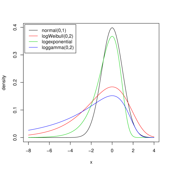
Figure 1: Density for some relevant members of the generalized loggamma family.

2 Robust estimation and inference

We condider the three parameter family $LG(\mu,\sigma,\lambda)$ with $\boldsymbol{\theta}=(\mu,\sigma,\lambda)$, and distribution function $F_{\boldsymbol{\theta}}(y)=F^{\ast}((y-\mu)/\sigma,\lambda)$. For $0<u<1$ let $Q(u,\boldsymbol{\theta})$ be the $u$-quantile of $F_{\boldsymbol{\theta}}(y)$. Then, $Q(u,\boldsymbol{\theta})=\sigma Q^{\ast}(u,\lambda)+\mu$, where $Q^{\ast}(u,\lambda)=Q(u,(0,1,\lambda))$. Let $y_{(1)},\cdots,y_{(n)}$ be the order statistics of a sample of size $n$ from $LG(\mu_{0},\sigma_{0},\lambda_{0})$, and $\boldsymbol{\theta}_{0}=(\mu_{0},\sigma_{0},\lambda_{0})$ is the unknow vector of parameters to be estimated. Since, $y_{(j)}$ is the quantile $u_{n,j}=(j-0.5)/n$ of the empirical distribution, it should be close to the corresponding theoretical quantile $\sigma_{0}Q^{\ast}(u_{n,j},\lambda_{0})+\mu_{0}$. Hence, the residuals:

$$r_{n,j}(\boldsymbol{\theta})=y_{(j)}-\mu-\sigma Q^{\ast}(u_{n,j},\lambda)$$

are a function of $\boldsymbol{\theta}$ and they should be as small as possible. To summarize their size a scale $s$ is often used. Given a sample $\mathbf{u}=(u_{1},\cdots,u_{n})$, $s$ is a function of $\mathbf{u}$ with two basic properties: (i) $s(\mathbf{u})\geq 0$; (ii) for any scalar $\gamma$, $s(\gamma\mathbf{u})=|\gamma|s(\mathbf{u})$. The most common scale is $\left(\sum_{j=1}^{n}u_{j}^{2}/n\right)^{1/2}$ and it is clearly non robust. To the aim of gaining robustness we use a $\tau$ scale $\tau(r_{n,1}(\boldsymbol{\theta}),\cdots,r_{n,n}(\boldsymbol{\theta}))$ introduced by Yohai and Zamar [1988]. A short review of $\tau$ scales can be found in Appendix A.

Then, the Q$\tau$ estimator is defined by

$$\tilde{\boldsymbol{\theta}}=\arg\min_{\boldsymbol{\theta}}\tau\left(r_{n,1}(\boldsymbol{\theta}),\cdots,r_{n,n}(\boldsymbol{\theta})\right)\ .$$

We note that, fixing $\lambda$, the value of $\mu$ and $\sigma$ minimizing the $\tau$ scale are obtained by a simple regression $\tau$ estimate for the responses $y_{(j)}$ and the regressors $Q^{\ast}(u_{n,j},\lambda)$. We also note [Serfling, 1980] that $n^{1/2}r_{n,j}(\boldsymbol{\theta}_{0})$ is approximately distributed according to $N(0,v^{2}(\boldsymbol{\theta}_{0},u_{n,j}))$, where

$$v^{2}(\boldsymbol{\theta}_{0},u)=\frac{\sigma_{0}^{2}u(1-u)}{f_{\lambda_{0}}^{2}(Q^{\ast}(u,\lambda_{0}))}\ .$$

Then, the variances of the regression errors can be estimated by

$$\tilde{\sigma}_{j}^{2}=v^{2}(\tilde{\boldsymbol{\theta}}_{n},u_{n,j})$$

and the basic estimator can be improved by means of a weighted procedure. More precisely, one defines the weighted Q$\tau$ estimator (WQ$\tau$), with the set of weights $1/\tilde{\sigma}_{1},\cdots,\tilde{\sigma}_{n}$, by

$$\tilde{\boldsymbol{\theta}}^{w}=\arg\min_{\boldsymbol{\theta}}\tau\left(\frac{r_{n,1}(\boldsymbol{\theta})}{\tilde{\sigma}_{1}},\cdots,\frac{r_{n,n}(\boldsymbol{\theta})}{\tilde{\sigma}_{n}}\right)\ .$$

Monte Carlo simulations [Agostinelli et al., 2014] show that both the Q$\tau$ and the WQ$\tau$ estimators perform well in the case the model is correct and also when the sample contains outliers. These empirical findings are corroborated by a theoretical results showing that Q$\tau$ and WQ$\tau$ have a $50\%$ break down point (BDP) (according to a special definition of BDP - the finite sample distribution break down point - which is particularly designed to asses the degree of global stability of a distribution estimate).

2.1 Weighted likelihood estimators

Unfortunately, Q$\tau$ and WQ$\tau$ are not asymptotically normal and therefore inconvenient for inference. Their rates of convergence is however of order $n^{1/2}$ and this makes them a good starting point for a one-step weighted likelihood (WL) procedure which is asymptotically normal and fully efficient at the model. The package robustloggamma implements two WL estimators: the fully iterated weighted likelihood and the one step weighted likelihood. Monte Carlo simulations [Agostinelli et al., 2014] show that both these estimators maintain the robust properties (BDP) of Q$\tau$ and WQ$\tau$.

In general, a weighted likelihood estimator (WLE) as defined in Markatou et al. [1998] is a solution of the following estimating equations

$$\frac{1}{n}\sum_{j=1}^{n}w(y_{j},\boldsymbol{\theta})\mathbf{z}(y_{j},\boldsymbol{\theta})=\mathbf{0}\ ,$$

where $\mathbf{z}(y,\boldsymbol{\theta})$ is the usual score function vector and $w(y,\boldsymbol{\theta})$ is a weight function defined by

$$w(y,\boldsymbol{\theta})=\min\left(1,\frac{\left[A(\delta(y,\boldsymbol{\theta}))+1\right]^{+}}{\delta(y,\boldsymbol{\theta})+1}\right)\ ,$$

where $\delta(y,\boldsymbol{\theta})$ is the Pearson residual [Lindsay, 1994], measuring the agreement between the distribution of the data and the assumed model. It is defined as $\delta(y,\boldsymbol{\theta})=\left[f^{\ast}(y)-f_{\boldsymbol{\theta}}^{\ast}(y)\right]/f_{\boldsymbol{\theta}}^{\ast}(y)$, where $f^{\ast}(y)=\int k(y,t,h)\ dF_{n}(t)$ is a kernel density estimate of $f_{\boldsymbol{\theta}}$ (with bandwidth $h$), $f_{\boldsymbol{\theta}}^{\ast}(y)=\int k(y,t,h)f_{\boldsymbol{\theta}}(t)\ dt$ is the corresponding smoothed model density, $F_{n}$ is the empirical cumulative distribution function, and $[x]^{+}=\max(0,x)$.

The function $A(\cdot)$ is called residual adjustment function (RAF). When $A(\delta)=\delta$ the weights $w(y_{j},\boldsymbol{\theta})=1$ and the WLE equations coincides with classical MLE equations. Generally, the weight function $w$ uses RAF that correspond to minimum disparity problems [Lindsay, 1994], see Appendix B for some examples.

The fully iterated weighted likelihood estimator (FIWL) is the solution of the weighted equations, while the one-step weighted likelihood estimator (1SWL) is defined by

$$\hat{\boldsymbol{\theta}}=\tilde{\boldsymbol{\theta}}-\mathbf{J}^{-1}\sum_{j=1}^{n}w(y_{j},\tilde{\boldsymbol{\theta}})\mathbf{z}(y_{j},\tilde{\boldsymbol{\theta}})\ ,$$

where $\mathbf{J}=\int w(y,\tilde{\boldsymbol{\theta}})\nabla\mathbf{z}(y,\tilde{\boldsymbol{\theta}})\ dF_{\tilde{\boldsymbol{\theta}}}(y)$ and $\nabla$ denotes differentiation with respect to $\boldsymbol{\theta}$. This definition is similar to a Fisher scoring step, where an extra term obtained by differentiating the weight with respect to $\boldsymbol{\theta}$ is dropped since, when evaluated at the model, is equal to zero. Further information on minimum distance methods and weighted likelihood procedures are available in Basu et al. [2011].

3 Algorithms and implementation

In the following sections, we describe the computation of the estimators implemented in the main function loggammarob. We first recall its arguments, a reference chart is reported in the Appendix C. The only required argument is x which contains the data set in a numeric vector. The argument method allows to choose among the available robust procedures. The default method is "oneWL", a one step weighted likelihood estimator starting from WQ$\tau$. Other alternatives are "QTau" (Q$\tau$), "WQTau" (WQ$\tau$), "WL" (Fully iterated weighed likelihood) and "ML" (Maximum likelihood). When method is not Q$\tau$ an optional numeric vector of length $3$ (location, scale, shape) could be supplied in the argument start to be used as starting value, otherwise, the default is WQ$\tau$ for the likelihood based methods and Q$\tau$ for WQ$\tau$. By default, weights in the WQ$\tau$ are specified as described in the previous section, if a different set of weights are needed the weights argument could be used. Fine tuning parameters are set by the function loggammarob.control and passed to the main function by the control parameter.

3.1 Computation of Q$\tau$ and WQ$\tau$

To optimize the $\tau$ scale for a given value of $\lambda$, robustloggamma uses the resampling algorithm described in Salibian-Barrera et al. [2008]. Let $x_{j}=Q^{\ast}(u_{n,j},\lambda)$ and consider the following steps:

1. Take a random subsample of size $2$ made of the pairs $(x_{(j_{1})},y_{(j_{1})})$ and $(x_{(j_{2})},y_{(j_{2})})$.

2. Compute a preliminary estimate of $\mu$ and $\sigma$ of the form

   $$\sigma^{(0)}=\frac{y_{(j_{1})}-y_{(j_{2})}}{x_{(j_{1})}-x_{(j_{2})}}\qquad\qquad\mu^{(0)}=y_{(j_{1})}-\sigma_{i}^{(0)}x_{(j_{1})}$$

3. Compute the residuals $r_{j}^{(0)}=y_{(j)}-\sigma^{(0)}x_{j}-\mu^{(0)}$ for $j=1,...,n$.

4. Compute least squares estimates $\mu^{(1)}$, $\sigma^{(1)}$ based on the $n/2$ pairs with the smallest absolute residuals $r_{j}^{(0)}$.

5. Compute the residuals $r_{j}^{(1)}$ for $j=1,...,n$ and the $\tau$ scale $\tau(r_{1}^{(1)},\cdots,r_{n}^{(1)})$.

Steps 1-5 are repeated a large number $N$ of times and the values $\mu^{(1)}$, $\sigma^{(1)}$ corresponding to the minimal $\tau$ scale are retained. These values are then used as starting values of an IRWLS algorithm, where the weights are defined, at each iteration, as $w_{j}=W\phi_{j1}+\phi_{j2}$ and

$$W =\frac{\sum_{j=1}^{n}2\rho_{2}(r_{j}/s)-\psi_{2}(r_{j}/s)r_{j}/s}{\sum_{j=1}^{n}\psi_{1}(r_{j}/s)r_{j}/s},$$

$$\phi_{jk} =\psi_{k}(r_{j}/s)/(r_{j}/s),\qquad k=1,2\ ,$$

$\psi_{k}$ is the first derivative of the $\rho$ function $\rho_{k}$ (see Appendix A), and $s$ is a scale which is recursively updated as follows

$$s=s\left(\frac{2}{n}\sum_{j=1}^{n}\rho_{1}(r_{j}/s)\right)^{1/2}$$

with initial value $s=\text{median}(|r_{j}|)/0.6745$.

This algorithm is used to compute $\mu(\lambda)$ and $\sigma(\lambda)$ for all values of $\lambda$ in a given grid $\lambda_{1},\cdots,\lambda_{k}$. The final value of $\lambda$ is then obtained by minimizing the $\tau$ scale over the grid.

The first part of the algorithm is implemented in Fortran while the IRWLS algorithm is implemented in R. The initial random procedure uses the R uniform pseudo random number generator and can be controlled by setting the seed in the usual way. The function loggammarob.control is used to set all the other parameters. tuning.rho and tuning.psi set the constants $c_{1}$ and $c_{2}$ of the $\rho$ functions $\rho_{1}$ and $\rho_{2}$. nResample controls the number of subsamples $N$, max.it, and refine.tol provide the maximum number of iterations and the tolerance of the IRWLS algorithm. An equally spaced grid for $\lambda$ is defined by the arguments lower, upper and n with obvious meaning. Default values, for these parameters can be seen by

R> loggammarob.control() Once a Q$\tau$ estimate $\tilde{\boldsymbol{\theta}}$ is obtained, the WQ$\tau$ is easily computed by first evaluating a fixed set of scales

$$\tilde{\sigma}_{j}^{2}=v^{2}(\tilde{\boldsymbol{\theta}},u_{n,j})$$

then the IRWLS is used with $\tilde{\boldsymbol{\theta}}$ as starting value and $r_{j}/\tilde{\sigma}_{j}$ in place of $r_{j}$.

3.2 Computation of FIWL and 1SWL

Weights need to be evaluated for both 1SWL and FIWL. To compute the kernel density estimate $f^{\ast}(y)$, robustloggamma uses the function density with kernel="gaussian", cut=3, and n=512. The smoothed model $f_{\boldsymbol{\theta}}^{\ast}(y)$ is approximated by

$$\frac{1}{K}\sum_{k=1}^{K}k(y,y_{k},h),$$

where $y_{k}$ is the quantile of order $(k-0.5)/K$ of $F_{\tilde{\boldsymbol{\theta}}}$. The bandwidth $h$ is adaptively fixed to bw times the actual value of $\sigma$ and $K$ is controlled by the argument subdivisions. The RAF is fixed by raf among several choices: "NED" (negative exponential disparity), "GKL" (generalized Kullback-Leibler), "PWD" (power divergence measure), "HD" (Hellinger distance), "SCHI2" (symmetric Chi-Squared distance), and tau selects the particular member of the family in case of "GKL" and "PWD". Finally, weights smaller than minw are set to zero.

For 1SWL, $\mathbf{J}=\int w(y,\tilde{\boldsymbol{\theta}})\nabla\mathbf{z}(y,\tilde{\boldsymbol{\theta}})\ dF_{\tilde{\boldsymbol{\theta}}}(y)$ is approximated by

$$\frac{1}{K}\sum_{k=1}^{K}w(y_{k},\tilde{\boldsymbol{\theta}})\nabla\mathbf{z}(y_{k},\tilde{\boldsymbol{\theta}})\ .$$

Here $K$ is controlled by nexp. Furthermore, the step can be multiplied by the step argument (with default $1$).

4 An illustration

We illustrate the use of robustloggamma with the help of the data set drg2000 included in the package. The data refer to $70323$ stays that were observed in year $2000$ in a group of Swiss hospitals within a pilot study aimed at the implementation of a diagnosis-related grouping (DRG) system. DRG systems are used in modern hospital management to classify each individual stay into a group according to the patient characteristics. The classification rules are defined so that the groups are as homogeneous as possible with respect to clinical criteria (diagnoses and procedures) and to resource consumption. A mean cost of each group is usually estimated yearly with the help of available data about the observed stays on a national basis. This cost is then assigned to each stay in the same group and used for reimbursement and budgeting.

Cost distributions are typically skewed and often contain outliers. When a small number of outliers are observed, the classical estimates of the mean can be much different than when none is observed. And since the values and the frequency of outliers fluctuate from year to year, the classical mean cost is unreliable. Not surprisingly, since many DRGs must routinely be inspected each year, automatic outlier detection is a recurrent hot topic for discussion among hospital managers.

The data set has four variables: LOS length of stay, Cost cost of stay in Swiss francs, APDRG DRG code (according to the “All Patients DRG” system) and MDC Major diagnostic category. Packages xtable [Dahl, 2013] and lattice [Sarkar, 2008] will be used during the illustration.

R> require("xtable")R> require("lattice")R> data("drg2000") We will analyse the variable Cost on the logarithmic scale for the following four DRGs:

AP-DRG	Description
185	Dental & oral dis exc exctract & restorations, Age > 17
222	Knee procedures w/o cc
237	Sprain, strain, disloc of hip, pelvis, thigh
360	Vagina, Cervix & Vulva Procedures

R> APDRG <- c(185, 222, 237, 360)R> index <- unlist(sapply(APDRG, function(x) which(drg2000$APDRG==x)))R> DRG <- drg2000[index,]

Figure 2, obtained with the following code, shows a density plot for each selected DRG:

R> print(densityplot(~I(log(Cost)) | factor(APDRG), data=DRG,+                   plot.points="rug", ref=TRUE))

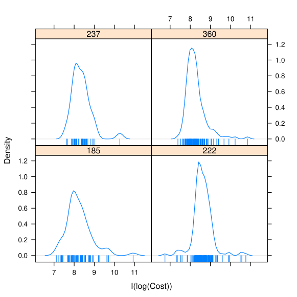
Figure 2: Estimated densities of log(Cost) for selected DRGs.

Summary statistics are:

R> lapply(split(DRG$Cost,DRG$APDRG), summary)

$`185`   Min. 1st Qu.  Median    Mean 3rd Qu.    Max.   1228    2645    3462    5059    5047   55770$`222`   Min. 1st Qu.  Median    Mean 3rd Qu.    Max.  849.2  4362.0  5288.0  6307.0  6801.0 47240.0$`237`   Min. 1st Qu.  Median    Mean 3rd Qu.    Max.   2038    3144    4100    4987    5169   28780$`360`   Min. 1st Qu.  Median    Mean 3rd Qu.    Max.   1620    2863    3502    4680    4428   51160 A comparison between classical and robust measures of spread, indicates important differences:

R> lapply(split(DRG$Cost,DRG$APDRG), function(x) c(sd(x), mad(x)))

$`185`[1] 6894.890 1374.874$`222`[1] 5095.599 1648.444$`237`[1] 4490.546 1494.891$`360`[1] 5066.084 1075.537 The differences are due to the presence of outliers. Therefore, it is convenient to analyze the data with the help of robust methods. To begin with, we use the function loggammarob to fit a generalized loggamma model to sample APDRG=185. This function provides robust estimates of the parameters $\mu$ (location), $\sigma$ (scale), and $\lambda$ (shape) using the default method 1SWL:

R> Cost185 <- sort(DRG$Cost[DRG$APDRG==185])R> est185 <- loggammarob(log(Cost185))R> est185

Call:loggammarob(x = log(Cost185))Location:  8.04  Scale:  0.4944  Shape:  -0.6437  E(exp(X)):  4381 In addition, a summary method is available to calculate confidence intervals (based on the Wald statistics) for the parameters and for selected model quantiles (argument p).

R> summary(est185, p=c(0.9, 0.95, 0.99))

Call:summary.loggammarob(object = est185, p = c(0.9, 0.95, 0.99))Location:  8.04 s.e.  0.09841( 7.847 ,  8.233 )95 percent confidence intervalScale:  0.4944 s.e.  0.05071( 0.395 ,  0.5938 )95 percent confidence intervalShape:  -0.6437 s.e.  0.3005( -1.233 ,  -0.05467 )95 percent confidence intervalMean(exp(X)):  4381 s.e.  426.7( 3545 ,  5218 )95 percent confidence intervalQuantile of order  0.9 :  8.932 s.e.  0.2337( 8.474 ,  9.39 )95 percent confidence intervalQuantile of order  0.95 :  9.2 s.e.  0.343( 8.528 ,  9.873 )95 percent confidence intervalQuantile of order  0.99 :  9.774 s.e.  0.6505( 8.499 ,  11.05 )95 percent confidence intervalRobustness weights: 54 weights are ~= 1. The remaining 15 ones are summarized as   Min. 1st Qu.  Median    Mean 3rd Qu.    Max.0.05591 0.74150 0.88590 0.77530 0.99800 0.99890 The function also provides the robust weights that allow outlier’s identification. For instance:

R> which(est185$weights < 0.1)

[1] 1 reports the indices of the observations with weights smaller than $0.1$, which in this case is the first one only.

Robust tests on one or more parameters can be performed by means of the weighted Wald test described in Agostinelli and Markatou [2001]. For this purpose, we use the function loggammarob.test. For instance, we test the hypothesis that the shape parameter is equal to zero, i.e., that the lognormal model is an acceptable one:

R> loggammarob.test(est185, lambda=0)

Weighted Wald Test based on oneWLdata:ww = 4.5876, df = 1, p-value = 0.0322alternative hypothesis: true shape is not equal to 095 percent confidence interval: -1.23270096 -0.05466982sample estimates:[1] -0.6436854 To test the hypothesis that the location is zero and the scale is one we use:

R> loggammarob.test(est185, mu=0, sigma=1) however, in these situations, the confidence intervals are not calculated.

The default estimation method in loggammarob is 1SWL (one-step weighted likelihood). However, alternative estimates are made available: Q$\tau$, WQ$\tau$, WL, and ML. Q$\tau$ and WQ$\tau$, typically used as starting values for the weighted likelihood procedures, are obtained as follows:

R> qtau185 <- summary(loggammarob(log(Cost185), method="QTau"))R> wqtau185 <- summary(loggammarob(log(Cost185), method="WQTau")) The fully iterated weighted likelihood (FIWL) and the one-step weighted likelihood estimates (1SWL) are obtained as follows:

R> fiwl185 <- summary(loggammarob(log(Cost185), method="WL"))R> oswl185 <- summary(loggammarob(log(Cost185), method="oneWL")) The maximum likelihood estimate is also available:

R> ml <- summary(loggammarob(log(Cost185), method="ML")) We now compare the four samples. For this purpose, the function analysis available in the Supplemental Material must be loaded before running the next command.

R> results <- sapply(APDRG, function(x) analysis(APDRG=x, data=DRG),+              simplify=FALSE)

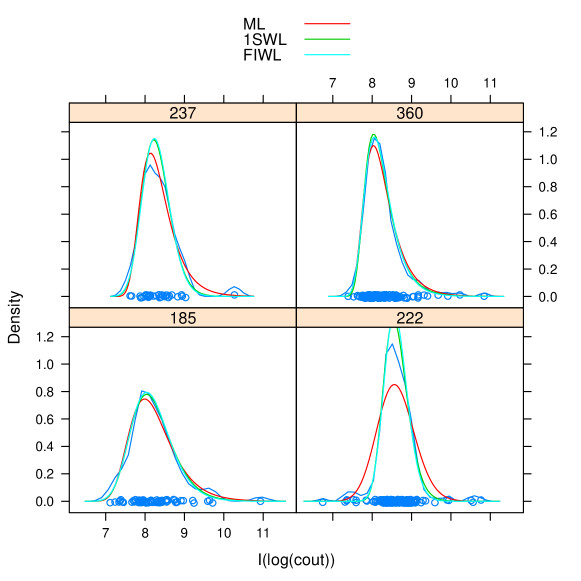
Figure 3: Estimated models provided by ML, 1SWL and FIWL for the four data sets.

Three estimated densities provided by ML, FIWL, and 1SWL are shown in Figure 3. The robust parameter estimates, their estimated standand errors, and their confidence intervals are shown in Table 1. The table was obtained with the help of the the function maketable available in the Supplemental Material.

DRG		ML				1SWL				FIWL
		$\mu$	$\sigma$	$\lambda$	$\eta$	$\mu$	$\sigma$	$\lambda$	$\eta$	$\mu$	$\sigma$	$\lambda$	$\eta$
185	est	7.989	0.501	-0.892	4837	8.04	0.494	-0.644	4381	8.043	0.489	-0.574	4232
	se	0.101	0.056	0.305	657	0.098	0.051	0.301	427	0.095	0.048	0.295	372
	left	7.792	0.392	-1.49	3550	7.847	0.395	-1.233	3545	7.856	0.394	-1.153	3504
	right	8.186	0.61	-0.295	6124	8.233	0.594	-0.055	5218	8.23	0.583	0.005	4961
222	est	8.563	0.467	-0.197	6152	8.544	0.295	-0.493	5836	8.566	0.289	-0.308	5747
	se	0.054	0.025	0.179	237	0.035	0.017	0.183	156	0.035	0.016	0.184	138
	left	8.457	0.419	-0.549	5687	8.475	0.261	-0.852	5531	8.498	0.257	-0.669	5475
	right	8.67	0.515	0.155	6618	8.613	0.329	-0.135	6141	8.634	0.321	0.054	6018
237	est	8.139	0.349	-1.05	4836	8.221	0.344	-0.432	4300	8.236	0.343	-0.329	4266
	se	0.103	0.059	0.455	596	0.095	0.046	0.423	308	0.095	0.045	0.425	290
	left	7.936	0.234	-1.942	3667	8.034	0.254	-1.261	3697	8.05	0.256	-1.162	3697
	right	8.341	0.465	-0.158	6005	8.408	0.434	0.396	4902	8.422	0.431	0.504	4835
360	est	8.034	0.324	-1.191	4444	8.038	0.304	-1.137	4235	8.055	0.318	-0.974	4142
	se	0.049	0.029	0.237	280	0.046	0.026	0.234	228	0.046	0.026	0.221	201
	left	7.938	0.268	-1.655	3896	7.949	0.252	-1.595	3789	7.965	0.267	-1.407	3748
	right	8.129	0.38	-0.727	4993	8.127	0.356	-0.679	4681	8.145	0.368	-0.542	4535

Table 1: Estimates, standard errors and confidence intervals for the four samples.

We note that outliers are present in all samples (Figure 4). However, for APDRG=185 and APDRG=360 they do not have a significant impact on the estimates and the associated inferences. On the contrary, for APDRG=222 the outliers markedly inflate the ML scale estimate and, for APDRG=237 a single outlier has a great impact on the ML estimate of lambda. For this sample, the robust parameter estimates and their confidence intervals suggest that the lognormal density is a possible model. To visualize the weights, we use the following code:

R> weights <- function(x, results) {+   os <- results[[x]]$os+   wl <- results[[x]]$wl+   ans <- t(cbind(os$weights, wl$weights, wl$data, x))+   return(ans)+ }R> w <- as.data.frame(matrix(unlist(sapply(1:4,+   function(x) weights(x, results=results))), ncol=4, byrow=TRUE))R> colnames(w) <- c("OSWL", "FIWL", "data", "drg")R> w$drg <- factor(w$drg, labels=APDRG)R> lattice.theme <- trellis.par.get()R> col <- lattice.theme$superpose.symbol$col[1:2]R> print(xyplot(OSWL+FIWL~data | drg, data=w, type="b",+   col=col, pch=21, key = list(text=list(c("1SWL", "FIWL")),+   lines=list(col=col)), xlab="log(Cost)", ylab="weights"))

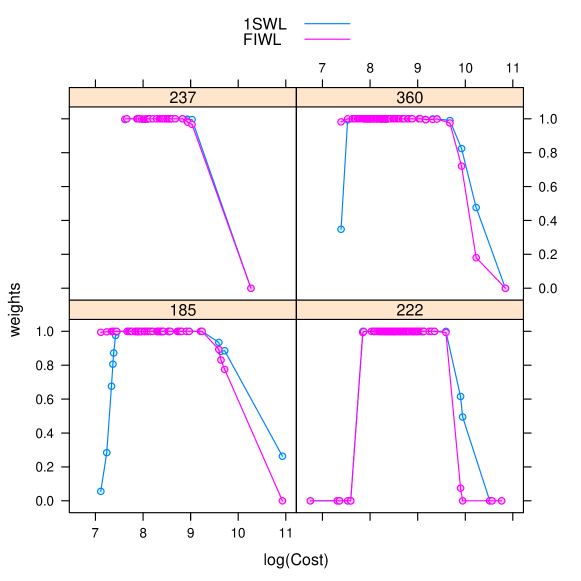
Figure 4: Weights provided by 1SWL and FIWL.

Is the two-parameter gamma distribution an acceptable model for the four samples? To answer this question, we test the hypothesis $\sigma=\lambda$. We use the function loggammarob.wilks with weights provided by ML, 1SWL and, FIWL. The results are summarized in Table 2 provided by the function extractwilks reported in the Supplemental Material. The hypothesis is always strongly rejected for DRGs 185, 222, 360. For DRG 237, the presence of outliers leads ML to stronlgy reject the hypothesis, while the robust methods accept it ($\mu_{0}$ and $\sigma_{0}=\lambda_{0}$ are the estimated parameters under the null hypothesis).

R> wilks <- extractwilks(results)R> wilks <- cbind(c("185", rep(" ", 3), "222", rep(" ", 3),+                    "237", rep(" ", 3), "360", rep(" ", 3)),+                rep(c("Statistic", "p-value", "$\\mu_0$",+                "$\\sigma_0$"),4), wilks)R> xwilks <- xtable(wilks)

DRG		ML	1SWL	FIWL
185	Statistic	45.882	29.1741	15.3918
	p-value	0	0	1e-04
	$\mu_{0}$	8.5288	8.4277	8.3497
	$\sigma_{0}$	0.7281	0.5949	0.5502
222	Statistic	52.3126	24.7645	10.8147
	p-value	0	0	0.001
	$\mu_{0}$	8.7494	8.6712	8.6563
	$\sigma_{0}$	0.5172	0.3208	0.2984
237	Statistic	23.1627	1.7348	1.7679
	p-value	0	0.1878	0.1836
	$\mu_{0}$	8.5146	8.3583	8.3567
	$\sigma_{0}$	0.5548	0.3527	0.3518
360	Statistic	123.933	75.6255	62.5466
	p-value	0	0	0
	$\mu_{0}$	8.4512	8.3543	8.3363
	$\sigma_{0}$	0.591	0.4654	0.4481

Table 2: Weighted Wilks test for the hypothesis $\sigma=\lambda$.

Finally, we draw Q-Q plots based on ML, 1SWL and FIWL (Figure 5) for the four data sets. Darker points are associated with smaller weights. $90\%$ confidence bands are provided to check the adequacy of the model to the data.

R> quant <- function(x, method, results) {+   res <- results[[x]][[method]]+   n <- length(res$data)+   q <- qloggamma(p=ppoints(n), mu=res$mu, sigma=res$sigma, lambda=res$lambda)+   qconf <- summary(res, p=ppoints(n), conf.level=0.90)$qconf.int+   ans <- t(cbind(q, qconf, res$data, res$weights, x, method))+   return(ans)+ }R> q1 <- matrix(unlist(sapply(1:4,+   function(x) quant(x, method=1, results=results))),+   ncol=7, byrow=TRUE)R> q2 <- matrix(unlist(sapply(1:4,+   function(x) quant(x, method=2, results=results))),+   ncol=7, byrow=TRUE)R> q3 <- matrix(unlist(sapply(1:4,+   function(x) quant(x, method=3, results=results))),+   ncol=7, byrow=TRUE)R> q <- as.data.frame(rbind(q1,q2,q3))R> colnames(q) <- c("q", "qlower", "qupper", "Cost",+   "weights", "drg", "method")R> q$drg <- factor(q$drg, labels=APDRG)R> q$method <- factor(q$method, labels=c("ML", "1SWL", "FIWL"))

R> print(xyplot(Cost~q | drg+method, data=q, xlab="Theoretical Quantiles",+   ylab="Empirical Quantiles", fill.color=grey(q$weights), q=q,+   panel=function(x, y, fill.color, ..., subscripts, q) {+     fill=fill.color[subscripts]+     q=q[subscripts,]+     panel.xyplot(x, y, pch=21, fill=fill, col="black", ...)+     panel.xyplot(x, y=q$qupper, type="l", col="grey75")+     panel.xyplot(x, y=q$qlower, type="l", col="grey75")+   }+ ))

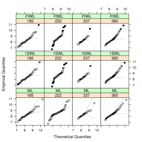
Figure 5: Q-Q plots and $90\%$ confidence bands (grey line). Darker points are associated with smaller weights.

5 Acknowledgments

All statistical analysis were performed on SCSCF (www.dais.unive.it/scscf), a multiprocessor cluster system owned by Ca’ Foscari University of Venice running under GNU/Linux.

This research was partially supported by the Italian-Argentinian project “Metodi robusti per la previsione del costo e della durata della degenza ospedaliera” funded in the collaboration program MINCYT-MAE AR14MO6.

Víctor Yohai research was partially supported by Grants 20020130100279 from Universidad of Buenos Aires, PIP 112-2008-01-00216 and 112-2011-01-00339 from CONICET and PICT 2011-0397 from ANPCYT.

Appendix A $\tau$ scale regression

In this appendix we briefly review the definition of $\tau$ scale and $\tau$ regression. For a detailed description see Maronna et al. [2006].

Let $\rho$ be a function satisfying the following properties: A: (i) $\rho(0)=0$; (ii) $\rho$ is even; (iii) if $|x_{1}|<|x_{2}|$, then $\rho(x_{1})\leq\rho(x_{2})$; (iv) $\rho$ is bounded; (v) $\rho$ is continuous.

Then, an M scale [Huber, 1981] based on $\rho$ is defined by the value $s$ satisfying

$$\frac{1}{n}\sum\limits_{j=1}^{n}\rho\left(\frac{u_{j}}{s}\right)=b\ ,$$

where $b$ is a given scalar and $0<b<a=\sup\rho$. Yohai and Zamar [1988] introduce the family of $\tau$ scales. A $\tau$ scale is based on two functions $\rho_{1}$ and $\rho_{2}$ satisfying properties A and such that $\rho_{2}\leq\rho_{1}$. To define a $\tau$ scale, one considers an M scale $s_{1}^{2}(\mathbf{u})$ based on $\rho_{1}$ then, the $\tau$ scale is given by

$$\tau^{2}(\mathbf{u})=s_{1}^{2}(\mathbf{u})\frac{1}{n}\sum_{j=1}^{n}\rho_{2}\left(\frac{u_{j}}{s_{1}(\mathbf{u})}\right)\ .$$

$\tau$ scale estimators can be extended easily to the linear regression case. Let us consider the regression model

$$y_{j}=\boldsymbol{\beta}^{t}\mathbf{x}_{j}+e_{j}\ ,\ 1\leq j\leq n\ ,$$

where $\boldsymbol{\beta}=(\beta_{1},\cdots,\beta_{p})^{t}$ and $\mathbf{x}_{j}=(x_{j1},\cdots,x_{jp})^{t}$. For a given $\boldsymbol{\beta}$, let $r_{j}(\boldsymbol{\beta})=y_{j}-\boldsymbol{\beta}^{t}\mathbf{x}_{j}$ be the corresponding residuals. The scale $\tau^{2}(r_{1}(\boldsymbol{\beta}),\cdots,r_{n}(\boldsymbol{\beta}))$ may be considered as a measure of goodness of fit. Based on this remark, Yohai and Zamar [1988] define robust estimators of the coefficients of a regression model by

$$\hat{\boldsymbol{\beta}}=\arg\min_{\boldsymbol{\beta}}\tau\left(r_{1}(\mathbf{\beta}),\cdots,r_{n}(\mathbf{\beta})\right)\ .$$

These estimators are called $\tau$ regression estimators. If $a/b=0.5$, the $\tau$ estimators have breakdown point (bdp) close to $50\%$ [Yohai and Zamar, 1988]. Moreover, we note that, if $\rho_{2}(u)=u^{2}$, $\tau^{2}(u_{1},\cdots,u_{n})=\text{ave}(u_{j}^{2})$ and then the regression $\tau$ estimator coincides with the least squares estimator. Therefore, taking as $\rho_{2}$ a bounded function close to the quadratic function, the regression $\tau$ estimators can be made arbitrarily efficient for normal errors. If the errors $e_{j}$ are heteroscedastic with variances proportional to $\sigma_{j}^{2}$, the efficiency of $\hat{\boldsymbol{\beta}}$ can be improved by means of a weighted procedure. A regression weighted $\tau$ estimator is given by

$$\hat{\boldsymbol{\beta}}=\arg\min_{\boldsymbol{\beta}}\tau\left(r_{1}^{\ast}(\boldsymbol{\beta}),\cdots,r_{n}^{\ast}(\boldsymbol{\beta})\right)\ ,$$

where $r_{j}^{\ast}(\boldsymbol{\beta})=r_{j}(\boldsymbol{\beta})/\sigma_{j}$.

Usually, one chooses $\rho_{1}$ and $\rho_{2}$ in the Tukey biweight family

$$\rho(u,c)=\left\{\begin{array}[]{lll}3(u/c)^{2}-3(u/c)^{4}+(u/c)^{6}&\text{if}&|u|\leq c\ ,\\ 1&\text{if}&|u|>c\ ,\end{array}\right.$$

using two values $c_{1}$ and $c_{2}$ of the tuning parameter $c$. For example, one can take $c_{1}=1.548$ and $c_{2}=6.08$. With $b=0.5$, these values yield regression estimators with breakdown point $0.5$ and normal efficiency of $95\%$.

Appendix B Residual adjustment functions

The literature provides several proposals for selecting the RAF. In the following, we recall two of them. The RAF based on the power divergence measure (PWD) [Cressie and Read, 1984, 1988], is given by

$$A_{pdm}(\delta,\tau)=\left\{\begin{array}[]{ll}\tau\left((\delta+1)^{1/\tau}-1\right)&\tau<\infty\\ \log(\delta+1)&\tau\rightarrow\infty\end{array}\right.$$

Special cases are maximum likelihood ($\tau=1$), Hellinger distance ($\tau=2$), Kullback–Leibler divergence ($\tau\rightarrow\infty$), and Neyman’s Chi–Square ($\tau=-1$). The RAF based on the generalized Kullback–Leibler divergence (GKL; Park and Basu [2003]) is given by:

$$A_{gkl}(\delta,\tau)=\frac{\log(\tau\delta+1)}{\tau}\qquad 0\leq\tau\leq 1\ .$$

Special cases are maximum likelihood ($\tau\rightarrow 0$) and Kullback–Leibler divergence ($\tau=1$). This RAF can be interpreted as a linear combination between the likelihood divergence and the Kullback–Leibler divergence. A further example is the RAF corresponding to the negative exponential dsparity (NED; [Lindsay, 1994])

$$A(\delta)=2-(2+\delta)\exp(-\delta)$$

which, for discrete models is second order efficient.

Appendix C Reference chart

Hereafter we provide the reference chart for the main function loggammarob. The usage has the following form

R> loggammarob(x, start=NULL, weights = rep(1, length(x)),+   method=c("oneWL", "WQTau", "WL", "QTau", "ML"), control, ...) where

x is a numeric vector, which contains the data.

start is NULL or a numeric vector containing the starting values of location, scale, and shape to be used when method is "WL", "oneWL" and "ML". Method "QTau" does not require starting values. When start is NULL, the methods "QTau" and "WQTau" are called in a series to compute the starting values.

weights is a numeric vector containing the weights for method "QTau".

method is a character string to select the method. The default is "oneWL" (one step weighted likelihood estimate starting from "WQTau"). Others available methods are "WL" (fully iterated weighted likelihood estimate), "WQTau" (weighted Q$\tau$ estimate), "QTau" (Q$\tau$ estimate), and "ML" (maximum likelihood estimate).

control is a list, which contains an object from the function loggammarob.control.

... further arguments that can be directly passed to the function.

The function returns an object of class ’loggammarob’. This is a list with the following components:

mu: location parameter estimate.

sigma: scale parameter estimate.

lambda: shape parameter estimate.

eta: estimate of E(exp(x)).

weights: the final weights.

iterations: number of iterations.

References

- Agostinelli and Markatou [2001] C. Agostinelli and M. Markatou. Test of hypotheses based on the weighted likelihood methodology. Statistica Sinica, 11(2):499–514, 2001.
- Agostinelli et al. [2014] C. Agostinelli, A. Marazzi, and V.J. Yohai. Robust estimation of the generalized loggamma model. Technometrics, 56(1):92–101, 2014. doi: 10.1080/00401706.2013.818578.
- Basu et al. [2011] A. Basu, H. Shioya, and C. Park. Statistical Inference: The Minimum Distance Approach. Chapman & Hall/CRC, Boca Raton, 2011.
- Cressie and Read [1984] N. Cressie and T.R.C. Read. Multinomial goodness–of–fit tests. Journal of the Royal Statistical Society B, 46:440–464, 1984.
- Cressie and Read [1988] N. Cressie and T.R.C. Read. Cressie–Read Statistic, pages 37–39. John Wiley & Sons, 1988. In: Encyclopedia of Statistical Sciences, Supplementary Volume, edited by S. Kotz and N.L. Johnson.
- Dahl [2013] D.B. Dahl. xtable: Export tables to LaTeX or HTML, 2013. URL http://CRAN.R-project.org/package=xtable. R package version 1.7-1.
- Huber [1981] P.J. Huber. Robust statistics. John Wiley & Sons, New York, 1981.
- Lawless [1980] J.F. Lawless. Inference in the generalized gamma and loggamma distributions. Technometrics, 22(3):409–419, 1980.
- Lindsay [1994] B.G. Lindsay. Efficiency versus robustness: The case for minimum hellinger distance and related methods. The Annals of Statistics, 22:1018–1114, 1994.
- Markatou et al. [1998] M. Markatou, A. Basu, and B.G. Lindsay. Weighted likelihood equations with bootstrap root search. Journal of the American Statistical Association, 93:740–750, 1998.
- Maronna et al. [2006] R.A. Maronna, D.R. Martin, and V.J. Yohai. Robust Statistics: Theory and Methods. John Wiley & Sons, New York, 2006.
- Park and Basu [2003] C. Park and A. Basu. The generalized kullback-leibler divergence and robust inference. Journal of Statistical Computation and Simulation, 73(5):311–332, 2003.
- Prentice [1974] R.L. Prentice. A loggamma model and its maximum likelihood estimation. Biometrika, 61(3):539–544, 1974.
- Salibian-Barrera et al. [2008] M. Salibian-Barrera, G. Willems, and R.H. Zamar. The fast-tau estimator for regression. Journal of Computational and Graphical Statistics, 17:659–682, 2008.
- Sarkar [2008] D. Sarkar. Lattice: Multivariate Data Visualization with R. Springer, New York, 2008. URL http://lmdvr.r-forge.r-project.org. ISBN 978-0-387-75968-5.
- Serfling [1980] R.J. Serfling. Approximation Theorems of Mathematical Statistics. John Wiley & Sons, New York, 1980.
- Stacy [1962] E.W. Stacy. A generalization of the gamma distribution. The Annals of Mathematical Statistics, 33:1187–1192, 1962.
- Yohai and Zamar [1988] V.J. Yohai and R.H. Zamar. High breakdown estimates of regression by means of the minimization of an efficient scale. Journal of the American Statistical Association, 83:406–413, 1988.