Risk-Constrained Reinforcement Learning
with Percentile Risk Criteria

Abstract

In many sequential decision-making problems one is interested in minimizing an expected cumulative cost while taking into account risk, i.e., increased awareness of events of small probability and high consequences. Accordingly, the objective of this paper is to present efficient reinforcement learning algorithms for risk-constrained Markov decision processes (MDPs), where risk is represented via a chance constraint or a constraint on the conditional value-at-risk (CVaR) of the cumulative cost. We collectively refer to such problems as percentile risk-constrained MDPs. Specifically, we first derive a formula for computing the gradient of the Lagrangian function for percentile risk-constrained MDPs. Then, we devise policy gradient and actor-critic algorithms that (1) estimate such gradient, (2) update the policy in the descent direction, and (3) update the Lagrange multiplier in the ascent direction. For these algorithms we prove convergence to locally optimal policies. Finally, we demonstrate the effectiveness of our algorithms in an optimal stopping problem and an online marketing application.

Keywords: Markov Decision Process, Reinforcement Learning, Conditional Value-at-Risk, Chance-Constrained Optimization, Policy Gradient Algorithms, Actor-Critic Algorithms

1 Introduction

The most widely-adopted optimization criterion for Markov decision processes (MDPs) is represented by the risk-neutral expectation of a cumulative cost. However, in many applications one is interested in taking into account risk, i.e., increased awareness of events of small probability and high consequences. Accordingly, in risk-sensitive MDPs the objective is to minimize a risk-sensitive criterion such as the expected exponential utility, a variance-related measure, or percentile performance. There are several risk metrics available in the literature, and constructing a “good” risk criterion in a manner that is both conceptually meaningful and computationally tractable remains a topic of current research.

Risk-Sensitive MDPs: One of the earliest risk metrics used for risk-sensitive MDPs is the exponential risk metric $(1/\gamma)\mathbb{E}\big{[}\exp(\gamma Z)\big{]}$, where $Z$ represents the cumulative cost for a sequence of decisions (Howard and Matheson, 1972). In this setting, the degree of risk-aversion is controlled by the parameter $\gamma$, whose selection, however, is often challenging. This motivated the study of several different approaches. In Collins (1997), the authors considered the maximization of a strictly concave functional of the distribution of the terminal state. In Wu and Lin (1999); Boda et al. (2004); Filar et al. (1995), risk-sensitive MDPs are cast as the problem of maximizing percentile performance. Variance-related risk metrics are considered, e.g., in Sobel (1982); Filar et al. (1989). Other mean, variance, and probabilistic criteria for risk-sensitive MDPs are discussed in the survey (White, 1988).

Numerous alternative risk metrics have recently been proposed in the literature, usually with the goal of providing an “intuitive” notion of risk and/or to ensure computational tractability. Value-at-risk (VaR) and conditional value-at-risk (CVaR) represent two promising such alternatives. They both aim at quantifying costs that might be encountered in the tail of a cost distribution, but in different ways. Specifically, for continuous cost distributions, VaR_α measures risk as the maximum cost that might be incurred with respect to a given confidence level $\alpha$. This risk metric is particularly useful when there is a well-defined failure state, e.g., a state that leads a robot to collide with an obstacle. A VaR_α constraint is often referred to as a chance (probability) constraint, especially in the engineering literature, and we will use this terminology in the remainder of the paper. In contrast, CVaR_α measures risk as the expected cost given that such cost is greater than or equal to VaR_α, and provides a number of theoretical and computational advantages. CVaR optimization was first developed by Rockafellar and Uryasev  (Rockafellar and Uryasev, 2002, 2000) and its numerical effectiveness has been demonstrated in several portfolio optimization and option hedging problems. Risk-sensitive MDPs with a conditional value at risk metric were considered in Boda and Filar (2006); Ott (2010); Bäuerle and Ott (2011), and a mean-average-value-at-risk problem has been solved in Bäuerle and Mundt (2009) for minimizing risk in financial markets.

The aforementioned works focus on the derivation of exact solutions, and the ensuing algorithms are only applicable to relatively small problems. This has recently motivated the application of reinforcement learning (RL) methods to risk-sensitive MDPs. We will refer to such problems as risk-sensitive RL.

Risk-Sensitive RL: To address large-scale problems, it is natural to apply reinforcement learning (RL) techniques to risk-sensitive MDPs. Reinforcement learning (Bertsekas and Tsitsiklis, 1996; Sutton and Barto, 1998) can be viewed as a class of sampling-based methods for solving MDPs. Popular reinforcement learning techniques include policy gradient (Williams, 1992; Marbach, 1998; Baxter and Bartlett, 2001) and actor-critic methods (Sutton et al., 2000; Konda and Tsitsiklis, 2000; Peters et al., 2005; Borkar, 2005; Bhatnagar et al., 2009; Bhatnagar and Lakshmanan, 2012), whereby policies are parameterized in terms of a parameter vector and policy search is performed via gradient flow approaches. One effective way to estimate gradients in RL problems is by simultaneous perturbation stochastic approximation (SPSA) (Spall, 1992). Risk-sensitive RL with expected exponential utility has been considered in  Borkar (2001, 2002). More recently, the works in  Tamar et al. (2012); Prashanth and Ghavamzadeh (2013) present RL algorithms for several variance-related risk measures, the works in Morimura et al. (2010); Tamar et al. (2015); Petrik and Subramanian (2012) consider CVaR-based formulations, and the works in Tallec (2007); Shapiro et al. (2013) consider nested CVaR-based formulations.

Risk-Constrained RL and Paper Contributions: Despite the rather large literature on risk-sensitive MDPs and RL, risk-constrained formulations have largely gone unaddressed, with only a few exceptions, e.g., Chow and Pavone (2013); Borkar and Jain (2014). Yet constrained formulations naturally arise in several domains, including engineering, finance, and logistics, and provide a principled approach to address multi-objective problems. The objective of this paper is to fill this gap by devising policy gradient and actor-critic algorithms for risk-constrained MDPs, where risk is represented via a constraint on the conditional value-at-risk (CVaR) of the cumulative cost or as a chance constraint. Specifically, the contribution of this paper is fourfold.

1. We formulate two risk-constrained MDP problems. The first one involves a CVaR constraint and the second one involves a chance constraint. For the CVaR-constrained optimization problem, we consider both discrete and continuous cost distributions. By re-writing the problems using a Lagrangian formulation, we derive for both problems a Bellman optimality condition with respect to an augmented MDP whose state consists of two parts, with the first part capturing the state of the original MDP and the second part keeping track of the cumulative constraint cost.

2. We devise a trajectory-based policy gradient algorithm for both CVaR-constrained and chance-constrained MDPs. The key novelty of this algorithm lies in an unbiased gradient estimation procedure under Monte Carlo sampling. Using an ordinary differential equation (ODE) approach, we establish convergence of the algorithm to locally optimal policies.

3. Using the aforementioned Bellman optimality condition, we derive several actor-critic algorithms to optimize policy and value function approximation parameters in an online fashion. As for the trajectory-based policy gradient algorithm, we show that the proposed actor-critic algorithms converge to locally optimal solutions.

4. We demonstrate the effectiveness of our algorithms in an optimal stopping problem as well as in a realistic personalized advertisement recommendation (ad recommendation) problem (see Derfer et al. (2007) for more details). For the latter problem, we empirically show that our CVaR-constrained RL algorithms successfully guarantee that the worst-case revenue is lower-bounded by the pre-specified company yearly target.

The rest of the paper is structured as follows. In Section 2 we introduce our notation and rigorously state the problem we wish to address, namely risk-constrained RL. The next two sections provide various RL methods to approximately compute (locally) optimal policies for CVaR constrained MDPs. A trajectory-based policy gradient algorithm is presented in Section 3 and its convergence analysis is provided in Appendix A (Appendix A.1 provides the gradient estimates of the CVaR parameter, the policy parameter, and the Lagrange multiplier, and Appendix A.2 gives their convergence proofs). Actor-critic algorithms are presented in Section 4 and their convergence analysis is provided in Appendix B (Appendix B.1 derives the gradient of the Lagrange multiplier as a function of the state-action value function, Appendix B.2.1 analyzes the convergence of the critic, and Appendix B.2.2 provides the multi-timescale convergence results of the CVaR parameter, the policy parameter, and the Lagrange multiplier). Section 5 extends the above policy gradient and actor-critic methods to the chance-constrained case. Empirical evaluation of our algorithms is the subject of Section 6. Finally, we conclude the paper in Section 7, where we also provide directions for future work.

This paper generalizes earlier results by the authors presented in Chow and Ghavamzadeh (2014).

2 Preliminaries

We begin by defining some notation that is used throughout the paper, as well as defining the problem addressed herein and stating some basic assumptions.

2.1 Notation

We consider decision-making problems modeled as a finite MDP ( an MDP with finite state and action spaces). A finite MDP is a tuple $(\mathcal{X},\mathcal{A},C,D,P,P_{0})$ where $\mathcal{X}=\{1,\ldots,n,{\color[rgb]{0,0,0}x_{\text{Tar}}}\}$ and $\mathcal{A}=\{1,\ldots,m\}$ are the state and action spaces, ${\color[rgb]{0,0,0}x_{\text{Tar}}}$ is a recurrent target state, and for a state $x$ and an action $a$, $C(x,a)$ is a cost function with $|C(x,a)|\leq C_{\max}$, $D(x,a)$ is a constraint cost function with $|D(x,a)|\leq D_{\max}$ , $P(\cdot|x,a)$ is the transition probability distribution, and $P_{0}(\cdot)$ is the initial state distribution. For simplicity, in this paper we assume $P_{0}=\mathbf{1}\{x=x^{0}\}$ for some given initial state $x^{0}\in\{1,\ldots,n\}$. Generalizations to non-atomic initial state distributions are straightforward, for which the details are omitted for the sake of brevity. A stationary policy $\mu(\cdot|x)$ for an MDP is a probability distribution over actions, conditioned on the current state. In policy gradient methods, such policies are parameterized by a $\kappa$-dimensional vector $\theta$, so the space of policies can be written as $\big{\{}\mu(\cdot|x;\theta),x\in\mathcal{X},\theta\in\Theta\subseteq R^{\kappa}\big{\}}$. Since in this setting a policy $\mu$ is uniquely defined by its parameter vector $\theta$, policy-dependent functions can be written as a function of $\mu$ or $\theta$, and we use $\mu(\cdot|x;\theta)$ to denote the policy and $\theta$ to denote the dependency on the policy (parameter).

Given a fixed $\gamma\in(0,1)$, we denote by $d_{\gamma}^{\mu}(x|x^{0})=(1-\gamma)\sum_{k=0}^{\infty}\gamma^{k}\mathbb{P}(x_{k}=x|x_{0}=x^{0};\mu)$ and $\pi_{\gamma}^{\mu}(x,a|x^{0})=d_{\gamma}^{\mu}(x|x^{0})\mu(a|x)$, the $\gamma$-discounted occupation measure of state $x$ and state-action pair $(x,a)$ under policy $\mu$, respectively. This occupation measure is a $\gamma$-discounted probability distribution for visiting each state and action pair, and it plays an important role in sampling states and actions from the real system in policy gradient and actor-critic algorithms, and in guaranteeing their convergence. Because the state and action spaces are finite, Theorem 3.1 in Altman (1999) shows that the occupation measure $d_{\gamma}^{\mu}(x|x^{0})$ is a well-defined probability distribution. On the other hand, when $\gamma=1$ the occupation measure of state $x$ and state-action pair $(x,a)$ under policy $\mu$ are respectively defined by $d^{\mu}(x|x^{0})=\sum_{t=0}^{\infty}\mathbb{P}(x_{t}=x|x^{0};\mu)$ and $\pi^{\mu}(x,a|x^{0})=d^{\mu}(x|x^{0})\mu(a|x)$. In this case the occupation measures characterize the total sums of visiting probabilities (although they are not in general probability distributions themselves) of state $x$ and state-action pair $(x,a)$. To study the well-posedness of the occupation measure, we define the following notion of a transient MDP.

Definition 1

Define $\mathcal{X}^{\prime}=\mathcal{X}\setminus\{{\color[rgb]{0,0,0}x_{\text{Tar}}}\}=\{1,\ldots,n\}$ as a state space of transient states. An MDP is said to be transient if,

1. $\sum_{k=0}^{\infty}\mathbb{P}(x_{k}=x|x^{0},\mu)<\infty$ for every $x\in\mathcal{X}^{\prime}$ and every stationary policy $\mu$,

2. $P({\color[rgb]{0,0,0}x_{\text{Tar}}}|{\color[rgb]{0,0,0}x_{\text{Tar}}},a)=1$ for every admissible control action $a\in\mathcal{A}$.

Furthermore let $T_{\mu,x}$ be the first-hitting time of the target state $x_{\text{Tar}}$ from an arbitrary initial state $x\in\mathcal{X}$ in the Markov chain induced by transition probability $P(\cdot|x,a)$ and policy $\mu$. Although transience implies the first-hitting time is square integrable and finite almost surely, we will make the stronger assumption (which implies transience) on the uniform boundedness of the first-hitting time.

Assumption 2

The first-hitting time $T_{\mu,x}$ is bounded almost surely over all stationary policies $\mu$ and all initial states $x\in\mathcal{X}$. We will refer to this upper bound as $T$, i.e., $T_{\mu,x}\leq T$ almost surely.

The above assumption can be justified by the fact that sample trajectories collected in most reinforcement learning algorithms (including policy gradient and actor-critic methods) consist of bounded finite stopping time (also known as a time-out). Note that although a bounded stopping time would seem to conflict with the time-stationarity of the transition probabilities, this can be resolved by augmenting the state space with a time-counter state, analogous to the arguments given in Section 4.7 in Bertsekas (1995).

Finally, we define the constraint and cost functions. Let $Z$ be a finite-mean ($\mathbb{E}[|Z|]<\infty$) random variable representing cost, with the cumulative distribution function ${\color[rgb]{0,0,0}F_{Z}(z)}=\mathbb{P}(Z\leq z)$ (e.g., one may think of $Z$ as the total cost of an investment strategy $\mu$). We define the value-at-risk at confidence level $\alpha\in(0,1)$ as

$$\text{VaR}_{\alpha}(Z)=\min\big{\{}z\mid{\color[rgb]{0,0,0}F_{Z}(z)}\geq\alpha\big{\}}.$$

Here the minimum is attained because $F_{Z}$ is non-decreasing and right-continuous in $z$. When $F_{Z}$ is continuous and strictly increasing, VaR${}_{\alpha}(Z)$ is the unique $z$ satisfying ${\color[rgb]{0,0,0}F_{Z}(z)}=\alpha$. As mentioned, we refer to a constraint on the VaR as a chance constraint.

Although VaR is a popular risk measure, it is not a coherent risk measure (Artzner et al., 1999) and does not quantify the costs that might be suffered beyond its value in the $\alpha$-tail of the distribution (Rockafellar and Uryasev, 2000), Rockafellar and Uryasev (2002). In many financial applications such as portfolio optimization where the probability of undesirable events could be small but the cost incurred could still be significant, besides describing risk as the probability of incurring costs, it will be more interesting to study the cost in the tail of the risk distribution. In this case, an alternative measure that addresses most of the VaR’s shortcomings is the conditional value-at-risk, defined as (Rockafellar and Uryasev, 2000)

$$\text{CVaR}_{\alpha}(Z):=\min_{\nu\in}\Big{\{}\nu+\frac{1}{1-\alpha}\mathbb{E}\big{[}(Z-\nu)^{+}\big{]}\Big{\}},$$ (1)

where $(x)^{+}=\max(x,0)$ represents the positive part of $x$. While it might not be an immediate observation, it has been shown in Theorem 1 of Rockafellar and Uryasev (2000) that the CVaR of the loss random variable $Z$ is equal to the average of the worst-case $\alpha$-fraction of losses.

We define the parameter $\gamma\in(0,1]$ as the discounting factor for the cost and constraint cost functions. When $\gamma<1$, we are aiming to solve the MDP problem with more focus on optimizing current costs over future costs. For a policy $\mu$, we define the cost of a state $x$ (state-action pair $(x,a)$) as the sum of (discounted) costs encountered by the decision-maker when it starts at state $x$ (state-action pair $(x,a)$) and then follows policy $\mu$, i.e.,

$${\color[rgb]{0,0,0}\mathcal{G}}^{\theta}(x)=\sum_{k=0}^{T-1}\gamma^{k}C(x_{k},a_{k})\mid x_{0}=x,\;{\color[rgb]{0,0,0}\mu(\cdot|\cdot,\theta)},\quad\quad{\color[rgb]{0,0,0}\mathcal{J}}^{\theta}(x)=\sum_{k=0}^{T-1}\gamma^{k}D(x_{k},a_{k})\mid x_{0}=x,\;{\color[rgb]{0,0,0}\mu(\cdot|\cdot,\theta)},$$

and

$$\begin{split}{\color[rgb]{0,0,0}\mathcal{G}}^{\theta}(x,a)=\sum_{k=0}^{T-1}\gamma^{k}C(x_{k},a_{k})\mid x_{0}=x,\;a_{0}=a,\;{\color[rgb]{0,0,0}\mu(\cdot|\cdot,\theta)},\\ {\color[rgb]{0,0,0}\mathcal{J}}^{\theta}(x,a)=\sum_{k=0}^{T-1}\gamma^{k}D(x_{k},a_{k})\mid x_{0}=x,\;a_{0}=a,\;{\color[rgb]{0,0,0}\mu(\cdot|\cdot,\theta)}.\end{split}$$

The expected values of the random variables ${\color[rgb]{0,0,0}\mathcal{G}}^{\theta}(x)$ and ${\color[rgb]{0,0,0}\mathcal{G}}^{\theta}(x,a)$ are known as the value and action-value functions of policy $\mu$, and are denoted by

$$V^{\theta}(x)=\mathbb{E}\big{[}{\color[rgb]{0,0,0}\mathcal{G}}^{\theta}(x)\big{]},\qquad\qquad Q^{\theta}(x,a)=\mathbb{E}\big{[}{\color[rgb]{0,0,0}\mathcal{G}}^{\theta}(x,a)\big{]}.$$

2.2 Problem Statement

The goal for standard discounted MDPs is to find an optimal policy that solves

$$\theta^{*}=\operatornamewithlimits{argmin}_{\theta}V^{\theta}(x^{0}).$$

For CVaR-constrained optimization in MDPs, we consider the discounted cost optimization problem with $\gamma\in(0,1)$, i.e., for a given confidence level $\alpha\in(0,1)$ and cost tolerance $\beta\in$,

$$\min_{\theta}V^{\theta}(x^{0})\quad\quad\text{{\color[rgb]{0,0,0} subject to}}\quad\quad\text{CVaR}_{\alpha}\big{(}{\color[rgb]{0,0,0}\mathcal{J}}^{\theta}(x^{0})\big{)}\leq\beta.$$ (2)

Using the definition of $H_{\alpha}(Z,\nu)$, one can reformulate (2) as:

$$\min_{\theta,\nu}V^{\theta}(x^{0})\quad\quad\text{{\color[rgb]{0,0,0} subject to}}\quad\quad H_{\alpha}\big{(}{\color[rgb]{0,0,0}\mathcal{J}}^{\theta}(x^{0}),\nu\big{)}\leq\beta,$$ (3)

where

$$H_{\alpha}(Z,\nu):=\nu+\frac{1}{1-\alpha}\mathbb{E}\big{[}(Z-\nu)^{+}\big{]}.$$

The equivalence between problem (2) and problem (3) can be shown as follows. Let $\theta_{2}\in\Theta$ be any arbitrary feasible policy parameter of problem (2). With $\theta_{2}$, one can always construct $\nu_{2}=\text{VaR}_{\alpha}(\mathcal{J}^{\theta_{2}}(x^{0}))$, such that $(\theta_{2},\nu_{2})$ is feasible to problem (3). This in turn implies that the solution of (3) is less than the solution of (2). On the other hand, the following chain of inequalities holds for any $\nu\in$: $\text{CVaR}_{\alpha}\big{(}\mathcal{J}^{\theta}(x^{0})\big{)}\leq H_{\alpha}\big{(}\mathcal{J}^{\theta}(x^{0}),\nu\big{)}\leq\beta$. This implies that the feasible set of $\theta$ in problem (3) is a subset of the feasible set of $\theta$ in problem (2), which further indicates that the solution of problem (2) is less than the solution of problem (3). By combining both arguments, one concludes the equivalence relation of these two problems.

It is shown in Rockafellar and Uryasev (2000) and Rockafellar and Uryasev (2002) that the optimal $\nu$ actually equals VaR_α, so we refer to this parameter as the VaR parameter. Here we choose to analyze the discounted-cost CVaR-constrained optimization problem, i.e., with  $\gamma\in(0,1)$, as in many financial and marketing applications where CVaR constraints are used, it is more intuitive to put more emphasis on current costs rather than on future costs. The analysis can be easily generalized for the case where $\gamma=1$.

For chance-constrained optimization in MDPs, we consider the stopping cost optimization problem with $\gamma=1$, i.e.,  for a given confidence level $\beta\in(0,1)$ and cost tolerance $\alpha\in$,

$$\min_{\theta}V^{\theta}(x^{0})\quad\quad\text{{subject to}}\quad\quad\mathbb{P}\big{(}{\color[rgb]{0,0,0}\mathcal{J}}^{\theta}(x^{0})\geq\alpha\big{)}\leq\beta.$$ (4)

Here we choose $\gamma=1$ because in many engineering applications, where chance constraints are used to ensure overall safety, there is no notion of discounting since future threats are often as important as the current one. Similarly, the analysis can be easily extended to the case where $\gamma\in(0,1)$.

There are a number of mild technical and notational assumptions which we will make throughout the paper, so we state them here:

Assumption 3 (Differentiability)

For any state-action pair $(x,a)$, $\mu(a|x;\theta)$ is continuously differentiable in $\theta$ and $\nabla_{\theta}\mu(a|x;\theta)$ is a Lipschitz function in $\theta$ for every $a\in\mathcal{A}$ and $x\in\mathcal{X}$.

Assumption 4 (Strict Feasibility)

There exists a transient policy $\mu(\cdot|x;\theta)$ such that

$$H_{\alpha}\big{(}{\color[rgb]{0,0,0}\mathcal{J}}^{\theta}(x^{0}),\nu\big{)}<\beta$$

in the CVaR-constrained optimization problem, and $P\big{(}{\color[rgb]{0,0,0}\mathcal{J}}^{\theta}(x^{0})\geq\alpha\big{)}<\beta$ in the chance-constrained problem.

In the remainder of the paper we first focus on studying stochastic approximation algorithms for the CVaR-constrained optimization problem (Sections 3 and 4) and then adapt the results to the chance-constrained optimization problem in Section 5. Our solution approach relies on a Lagrangian relaxation procedure, which is discussed next.

2.3 Lagrangian Approach and Reformulation

To solve (3), we employ a Lagrangian relaxation procedure (Chapter 3 of Bertsekas (1999)), which leads to the unconstrained problem:

$$\max_{\lambda\geq 0}\min_{\theta,\nu}\bigg{(}L(\nu,\theta,\lambda):=V^{\theta}(x^{0})+\lambda\Big{(}H_{\alpha}\big{(}{\color[rgb]{0,0,0}\mathcal{J}}^{\theta}(x^{0}),\nu\big{)}-\beta\Big{)}\bigg{)},$$ (5)

where $\lambda$ is the Lagrange multiplier. Notice that $L(\nu,\theta,\lambda)$ is a linear function in $\lambda$ and $H_{\alpha}\big{(}{\color[rgb]{0,0,0}\mathcal{J}}^{\theta}(x^{0}),\nu\big{)}$ is a continuous function in $\nu$. The saddle point theorem from Chapter 3 of Bertsekas (1999) states that a local saddle point $(\nu^{*},\theta^{*},\lambda^{*})$ for the maximin optimization problem $\max_{\lambda\geq 0}\min_{\theta,\nu}L(\nu,\theta,\lambda)$ is indeed a locally optimal policy $\theta^{*}$ for the CVaR-constrained optimization problem. To further explore this connection, we first have the following definition of a saddle point:

Definition 5

A local saddle point of $L(\nu,\theta,\lambda)$ is a point $(\nu^{*},\theta^{*},\lambda^{*})$ such that for some $r>0$, $\forall(\theta,\nu)\in\Theta\times\left[-\frac{D_{\max}}{1-\gamma},\frac{D_{\max}}{1-\gamma}\right]\cap\mathcal{B}_{(\theta^{*},\nu^{*})}(r)$ and $\forall\lambda\geq 0$, we have

$$L(\nu,\theta,\lambda^{*})\geq L(\nu^{*},\theta^{*},\lambda^{*})\geq L(\nu^{*},\theta^{*},\lambda),$$ (6)

where $\mathcal{B}_{(\theta^{*},\nu^{*})}(r)$ is a hyper-dimensional ball centered at $(\theta^{*},\nu^{*})$ with radius $r>0$.

In Chapter 7 of Ott (2010) and in Bäuerle and Ott (2011) it is shown that there exists a deterministic history-dependent optimal policy for CVaR-constrained optimization. The important point is that this policy does not depend on the complete history, but only on the current time step $k$, current state of the system $x_{k}$, and accumulated discounted constraint cost $\sum_{i=0}^{k}\gamma^{i}D(x_{k},a_{k})$.

In the following two sections, we present a policy gradient (PG) algorithm (Section 3) and several actor-critic (AC) algorithms (Section 4) to optimize (5) (and hence find a locally optimal solution to problem (3)). While the PG algorithm updates its parameters after observing several trajectories, the AC algorithms are incremental and update their parameters at each time-step.

3 A Trajectory-based Policy Gradient Algorithm

In this section, we present a policy gradient algorithm to solve the optimization problem (5). The idea of the algorithm is to descend in $(\theta,\nu)$ and ascend in $\lambda$ using the gradients of $L(\nu,\theta,\lambda)$ w.r.t. $\theta$, $\nu$, and $\lambda$, i.e.,

$$\nabla_{\theta}L(\nu,\theta,\lambda) =\nabla_{\theta}V^{\theta}(x^{0})+\frac{\lambda}{(1-\alpha)}\nabla_{\theta}\mathbb{E}\Big{[}\big{(}{\color[rgb]{0,0,0}\mathcal{J}}^{\theta}(x^{0})-\nu\big{)}^{+}\Big{]},$$ (7)

$$\partial_{\nu}L(\nu,\theta,\lambda) =\lambda\bigg{(}1+\frac{1}{(1-\alpha)}\partial_{\nu}\mathbb{E}\Big{[}\big{(}{\color[rgb]{0,0,0}\mathcal{J}}^{\theta}(x^{0})-\nu\big{)}^{+}\Big{]}\bigg{)}\ni\lambda\bigg{(}1-\frac{1}{(1-\alpha)}\mathbb{P}\big{(}{\color[rgb]{0,0,0}\mathcal{J}}^{\theta}(x^{0})\geq\nu\big{)}\bigg{)},$$ (8)

$$\nabla_{\lambda}L(\nu,\theta,\lambda) =\nu+\frac{1}{(1-\alpha)}\mathbb{E}\Big{[}\big{(}{\color[rgb]{0,0,0}\mathcal{J}}^{\theta}(x^{0})-\nu\big{)}^{+}\Big{]}-\beta.$$ (9)

The unit of observation in this algorithm is a trajectory generated by following the current policy. At each iteration, the algorithm generates $N$ trajectories by following the current policy, uses them to estimate the gradients in (7)–(9), and then uses these estimates to update the parameters $\nu,\theta,\lambda$.

Let $\xi=\{x_{0},a_{0},c_{0},x_{1},a_{1},c_{1},\ldots,x_{T-1},a_{T-1},c_{T-1},x_{T}\}$ be a trajectory generated by following the policy $\theta$, where $x_{T}={\color[rgb]{0,0,0}x_{\text{Tar}}}$ is the target state of the system. The cost, constraint cost, and probability of $\xi$ are defined as ${\color[rgb]{0,0,0}\mathcal{G}}(\xi)=\sum_{k=0}^{T-1}\gamma^{k}C(x_{k},a_{k})$, ${\color[rgb]{0,0,0}\mathcal{J}}(\xi)=\sum_{k=0}^{T-1}\gamma^{k}D(x_{k},a_{k})$, and $\mathbb{P}_{\theta}(\xi)=P_{0}(x_{0})\prod_{k=0}^{T-1}\mu(a_{k}|x_{k};\theta)P(x_{k+1}|x_{k},a_{k})$, respectively. Based on the definition of $\mathbb{P}_{\theta}(\xi)$, one obtains $\nabla_{\theta}\log\mathbb{P}_{\theta}(\xi)=\sum_{k=0}^{T-1}\nabla_{\theta}\log\mu(a_{k}|x_{k};\theta)$.

Algorithm 1 contains the pseudo-code of our proposed policy gradient algorithm. What appears inside the parentheses on the right-hand-side of the update equations are the estimates of the gradients of $L(\nu,\theta,\lambda)$ w.r.t. $\theta,\nu,\lambda$ (estimates of (7)–(9)). Gradient estimates of the Lagrangian function can be found in Appendix A.1. In the algorithm, $\Gamma_{\Theta}$ is an operator that projects a vector $\theta\in^{\kappa}$ to the closest point in a compact and convex set $\Theta\subset^{\kappa}$, i.e., $\Gamma_{\Theta}(\theta)=\arg\min_{\hat{\theta}\in\Theta}\|\theta-\hat{\theta}\|^{2}_{2}$, $\Gamma_{\mathcal{N}}$ is a projection operator to $[-\frac{D_{\max}}{1-\gamma},\frac{D_{\max}}{1-\gamma}]$, i.e., $\Gamma_{\mathcal{N}}(\nu)=\arg\min_{\hat{\nu}\in[-\frac{D_{\max}}{1-\gamma},\frac{D_{\max}}{1-\gamma}]}\|\nu-\hat{\nu}\|^{2}_{2}$, and $\Gamma_{\Lambda}$ is a projection operator to $[0,\lambda_{\max}]$, i.e., $\Gamma_{\Lambda}(\lambda)=\arg\min_{\hat{\lambda}\in[0,\lambda_{\max}]}\|\lambda-\hat{\lambda}\|^{2}_{2}$. These projection operators are necessary to ensure the convergence of the algorithm; see the end of Appendix A.2 for details. Next we introduce the following assumptions for the step-sizes of the policy gradient method in Algorithm 1.

Assumption 6 (Step Sizes for Policy Gradient)

The step size schedules $\{\zeta_{1}(k)\}$, $\{\zeta_{2}(k)\}$, and $\{\zeta_{3}(k)\}$ satisfy

$$\sum_{k}\zeta_{1}(k)=\sum_{k}\zeta_{2}(k)=\sum_{k}\zeta_{3}(k)=\infty,$$ (10)

$$\sum_{k}\zeta_{1}(k)^{2},\;\;\;\sum_{k}\zeta_{2}(k)^{2},\;\;\;\sum_{k}\zeta_{3}(k)^{2}<\infty,$$ (11)

$$\zeta_{1}(k)=o\big{(}\zeta_{2}(k)\big{)},\;\;\;\zeta_{2}(k)=o\big{(}\zeta_{3}(k)\big{)}.$$ (12)

These step-size schedules satisfy the standard conditions for stochastic approximation algorithms, and ensure that the $\nu$ update is on the fastest time-scale $\big{\{}\zeta_{3}(k)\big{\}}$, the policy $\theta$ update is on the intermediate time-scale $\big{\{}\zeta_{2}(k)\big{\}}$, and the Lagrange multiplier $\lambda$ update is on the slowest time-scale $\big{\{}\zeta_{1}(k)\big{\}}$. This results in a three time-scale stochastic approximation algorithm.

In the following theorem, we prove that our policy gradient algorithm converges to a locally optimal policy for the CVaR-constrained optimization problem.

Theorem 7

Under Assumptions 2–6, the sequence of policy updates in Algorithm 1 converges almost surely to a locally optimal policy $\theta^{*}$ for the CVaR-constrained optimization problem as $k$ goes to infinity.

While we refer the reader to Appendix A.2 for the technical details of this proof, a high level overview of the proof technique is given as follows.

1. First we show that each update of the multi-time scale discrete stochastic approximation algorithm $(\nu_{k},\theta_{k},\lambda_{k})$ converges almost surely, but at different speeds, to the stationary point $(\nu^{\ast},\theta^{*},\lambda^{*})$ of the corresponding continuous time system.

2. Then by using Lyapunov analysis, we show that the continuous time system is locally asymptotically stable at the stationary point $(\nu^{\ast},\theta^{*},\lambda^{*})$.

3. Since the Lyapunov function used in the above analysis is the Lagrangian function $L(\nu,\theta,\lambda)$, we finally conclude that the stationary point $(\nu^{\ast},\theta^{*},\lambda^{*})$ is also a local saddle point, which by the saddle point theorem (see e.g., Chapter 3 of Bertsekas (1999)), implies that $\theta^{*}$ is a locally optimal solution of the CVaR-constrained MDP problem (the primal problem).

This convergence proof procedure is standard for stochastic approximation algorithms, see (Bhatnagar et al., 2009; Bhatnagar and Lakshmanan, 2012; Prashanth and Ghavamzadeh, 2013) for more details, and represents the structural backbone for the convergence analysis of the other policy gradient and actor-critic methods provided in this paper.

  Input: parameterized policy $\mu(\cdot|\cdot;\theta)$, confidence level $\alpha$, and cost tolerance $\beta$

  Initialization: policy $\theta=\theta_{0}$, VaR parameter $\nu=\nu_{0}$, and the Lagrangian parameter $\lambda=\lambda_{0}$

  while TRUE do

     for $k=0,1,2,\ldots$ do

        Generate $N$ trajectories $\{\xi_{j,k}\}_{j=1}^{N}$ by starting at $x_{0}=x^{0}$ and following the current policy $\theta_{k}$.

$$\nu \nu_{k+1}=\Gamma_{\mathcal{N}}\bigg{[}\nu_{k}-\zeta_{3}(k)\bigg{(}\lambda_{k}-\frac{\lambda_{k}}{(1-\alpha)N}\sum_{j=1}^{N}\mathbf{1}\big{\{}{\color[rgb]{0,0,0}\mathcal{J}}(\xi_{j,k})\geq\nu_{k}\big{\}}\bigg{)}\bigg{]}$$ Update:

$$\theta \theta_{k+1}=\Gamma_{\Theta}\bigg{[}\theta_{k}-\zeta_{2}(k)\bigg{(}\frac{1}{N}\sum_{j=1}^{N}\nabla_{\theta}\log\mathbb{P}_{\theta}(\xi_{j,k})|_{\theta=\theta_{k}}{\color[rgb]{0,0,0}{\color[rgb]{0,0,0}\mathcal{G}}(\xi_{j,k})}$$ Update:

$$\hskip 21.68121pt+\frac{\lambda_{k}}{(1-\alpha)N}\sum_{j=1}^{N}\nabla_{\theta}\log\mathbb{P}_{\theta}(\xi_{j,k})|_{\theta=\theta_{k}}\big{(}{\color[rgb]{0,0,0}\mathcal{J}}(\xi_{j,k})-\nu_{k}\big{)}\mathbf{1}\big{\{}{\color[rgb]{0,0,0}\mathcal{J}}(\xi_{j,k})\geq\nu_{k}\big{\}}\bigg{)}\bigg{]}$$

$$\lambda \lambda_{k+1}=\Gamma_{\Lambda}\bigg{[}\lambda_{k}+\zeta_{1}(k)\bigg{(}\nu_{k}-\beta+\frac{1}{(1-\alpha)N}\sum_{j=1}^{N}\big{(}{\color[rgb]{0,0,0}\mathcal{J}}(\xi_{j,k})-\nu_{k}\big{)}\mathbf{1}\big{\{}{\color[rgb]{0,0,0}\mathcal{J}}(\xi_{j,k})\geq\nu_{k}\big{\}}\bigg{)}\bigg{]}$$ Update:

     end for

     if $\{\lambda_{k}\}$ converges to $\lambda_{\max}$, i.e., $|\lambda_{i^{*}}-\lambda_{\max}|\leq\epsilon$ for some tolerance parameter $\epsilon>0$ then

        Set $\lambda_{\max}\leftarrow 2\lambda_{\max}$.

     else

        return parameters $\nu,\theta,\lambda$ and break

     end if

  end while

Algorithm 1 Trajectory-based Policy Gradient Algorithm for CVaR MDP

Notice that the difference in convergence speeds between $\theta_{k}$, $\nu_{k}$, and $\lambda_{k}$ is due to the step-size schedules. Here $\nu$ converges faster than $\theta$ and $\theta$ converges faster than $\lambda$. This multi-time scale convergence property allows us to simplify the convergence analysis by assuming that $\theta$ and $\lambda$ are fixed in $\nu$’s convergence analysis, assuming that $\nu$ converges to $\nu^{*}(\theta)$ and $\lambda$ is fixed in $\theta$’s convergence analysis, and finally assuming that $\nu$ and $\theta$ have already converged to $\nu^{*}(\lambda)$ and $\theta^{*}(\lambda)$ in $\lambda$’s convergence analysis. To illustrate this idea, consider the following two-time scale stochastic approximation algorithm for updating $(x_{k},y_{k})\in\mathbf{X}\times\mathbf{Y}$:

$$x_{k+1} =x_{k}+\zeta_{1}(k)\big{(}f(x_{k},y_{k})+M_{k+1}\big{)},$$ (13)

$$y_{k+1} =y_{k}+\zeta_{2}(k)\big{(}g(x_{k},y_{k})+N_{k+1}\big{)},$$ (14)

where $f(x_{k},y_{k})$ and $g(x_{k},y_{k})$ are Lipschitz continuous functions, $M_{k+1}$, $N_{k+1}$ are square integrable Martingale differences w.r.t. the $\sigma$-fields $\sigma(x_{i},y_{i},M_{i},i\leq k)$ and $\sigma(x_{i},y_{i},N_{i},i\leq k)$, and $\zeta_{1}(k)$ and $\zeta_{2}(k)$ are non-summable, square summable step sizes. If $\zeta_{2}(k)$ converges to zero faster than $\zeta_{1}(k)$, then (13) is a faster recursion than (14) after some iteration $k_{0}$ (i.e., for $k\geq k_{0}$), which means (13) has uniformly larger increments than (14). Since (14) can be written as

$$y_{k+1}=y_{k}+\zeta_{1}(k)\Big{(}\frac{\zeta_{2}(k)}{\zeta_{1}(k)}\big{(}g(x_{k},y_{k})+N_{k+1}\big{)}\Big{)},$$

and by the fact that $\zeta_{2}(k)$ converges to zero faster than $\zeta_{1}(k)$, (13) and (14) can be viewed as noisy Euler discretizations of the ODEs $\dot{x}=f(x,y)$ and $\dot{y}=0$. Note that one can consider the ODE $\dot{x}=f(x,y_{0})$ in place of $\dot{x}=f(x,y)$, where $y_{0}$ is constant, because $\dot{y}=0$. One can then show (see e.g., Theorem 2 in Chapter 6 of Borkar (2008)) the main two-timescale convergence result, i.e., under the above assumptions associated with (14), the sequence $(x_{k},y_{k})$ converges to $\big{(}\mu(y^{\star}),y^{\star}\big{)}$ as $i\rightarrow\infty$, with probability one, where $\mu(y_{0})$ is a locally asymptotically stable equilibrium of the ODE $\dot{x}=f(x,y_{0})$, $\mu$ is a Lipschitz continuous function, and $y^{\star}$ is a locally asymptotically stable equilibrium of the ODE $\dot{y}=g\big{(}\mu(y),y\big{)}$.

4 Actor-Critic Algorithms

As mentioned in Section 3, the unit of observation in our policy gradient algorithm (Algorithm 1) is a system trajectory. This may result in high variance for the gradient estimates, especially when the length of the trajectories is long. To address this issue, in this section we propose two actor-critic algorithms that approximate some quantities in the gradient estimates by linear combinations of basis functions and update the parameters (linear coefficients) incrementally (after each state-action transition). We present two actor-critic algorithms for optimizing  (5). These algorithms are based on the gradient estimates of Sections 4.1-4.3. While the first algorithm (SPSA-based) is fully incremental and updates all the parameters $\theta,\nu,\lambda$ at each time-step, the second one updates $\theta$ at each time-step and updates $\nu$ and $\lambda$ only at the end of each trajectory, thus is regarded as a semi-trajectory-based method. Algorithm 2 contains the pseudo-code of these algorithms. The projection operators $\Gamma_{\Theta}$, $\Gamma_{\mathcal{N}}$, and $\Gamma_{\Lambda}$ are defined as in Section 3 and are necessary to ensure the convergence of the algorithms. At each step of our actor critic algorithms (steps indexed by $k$ in Algorithm 1 and in Algorithm 2) there are two parts:

• Inner loop (critic update): For a fixed policy (given as $\theta\in\Theta$), take action $a_{k}\sim\mu(\cdot|x_{k},s_{k};\theta_{k})$, observe the cost $c(x_{k},a_{k})$, the constraint cost $d(x_{k},a_{k})$, and the next state $(x_{k+1},s_{k+1})$. Using the method of temporal differences (TD) from Chapter 6 of Sutton and Barto (1998), estimate the value function $V^{\theta}(x,s)$.

• Outer loop (actor update): Estimate the gradient of $V^{\theta}(x,s)$ for policy parameter $\theta$, and hence the gradient of the Lagrangian $L(\nu,\theta,\lambda)$, using the unbiased sampling based point estimator for gradients with respect to $\theta$ and $\lambda$ and either: (1) using the SPSA method (20) to obtain an incremental estimator for gradient with respect to $\nu$ or (2) only calculating the gradient estimator with respect to $\nu$ at the end of the trajectory (see (23) for more details). Update the policy parameter $\theta\in\Theta$ in the descent direction, the VaR approximation $\nu\in\mathcal{N}$ in the descent direction, and the Lagrange multiplier $\lambda\in\Lambda$ in the ascent direction on specific timescales that ensure convergence to locally optimal solutions.

Next, we introduce the following assumptions for the step-sizes of the actor-critic method in Algorithm 2.

Assumption 8 (Step Sizes)

The step size schedules $\{\zeta_{1}(k)\}$, $\{\zeta_{2}(k)\}$, $\{\zeta_{3}(k)\}$, and $\{\zeta_{4}(k)\}$ satisfy

$$\sum_{k}\zeta_{1}(k)=\sum_{k}\zeta_{2}(k)=\sum_{k}\zeta_{3}(k)=\sum_{k}\zeta_{4}(k)=\infty,$$ (15)

$$\sum_{k}\zeta_{1}(k)^{2},\;\;\;\sum_{k}\zeta_{2}(k)^{2},\;\;\;\sum_{k}\zeta_{3}(k)^{2},\;\;\;\sum_{k}\zeta_{4}(k)^{2}<\infty,$$ (16)

$$\zeta_{1}(k)=o\big{(}\zeta_{2}(k)\big{)},\;\;\;\zeta_{2}(k)=o\big{(}\zeta_{3}(k)\big{)},\;\;\;\zeta_{3}(k)=o\big{(}\zeta_{4}(k)\big{)}.$$ (17)

Furthermore, the SPSA step size $\{\Delta_{k}\}$ in the actor-critic algorithm satisfies $\Delta_{k}\rightarrow 0$ as $k\rightarrow\infty$ and $\sum_{k}(\zeta_{2}(k)/\Delta_{k})^{2}<\infty$.

These step-size schedules satisfy the standard conditions for stochastic approximation algorithms, and ensure that the critic update is on the fastest time-scale $\big{\{}\zeta_{4}(k)\big{\}}$, the policy and VaR parameter updates are on the intermediate time-scale, with the $\nu$-update $\big{\{}\zeta_{3}(k)\big{\}}$ being faster than the $\theta$-update $\big{\{}\zeta_{2}(k)\big{\}}$, and finally the Lagrange multiplier update is on the slowest time-scale $\big{\{}\zeta_{1}(k)\big{\}}$. This results in four time-scale stochastic approximation algorithms.

  Input: Parameterized policy $\mu(\cdot|\cdot;\theta)$ and value function feature vector $\phi(\cdot)$ (both over the augmented MDP $\bar{\mathcal{M}}$), confidence level $\alpha$, and cost tolerance $\beta$

  Initialization: policy $\theta=\theta_{0}$; VaR parameter $\nu=\nu_{0}$; Lagrangian parameter $\lambda=\lambda_{0}$; value function weight vector $v=v_{0}$ ; initial condition $(x_{0},s_{0})=(x^{0},\nu)$

  while TRUE do

    // (1) SPSA-based Algorithm:

    for $k=0,1,2,\ldots$ do

       Draw action $\;a_{k}\sim\mu(\cdot|x_{k},s_{k};\theta_{k})$;                       Observe cost $\;\bar{C}_{\lambda_{k}}(x_{k},s_{k},a_{k})$;

       Observe next state $(x_{k+1},s_{k+1})\sim\bar{P}(\cdot|x_{k},s_{k},a_{k})$;   // note that $s_{k+1}=(s_{k}-D\big{(}x_{k},a_{k})\big{)}/\gamma\;$

       // AC Algorithm:

TD Error: $$\delta_{k}(v_{k})=\bar{C}_{\lambda_{k}}(x_{k},s_{k},a_{k})+\gamma v_{k}^{\top}\phi(x_{k+1},s_{k+1})-v_{k}^{\top}\phi(x_{k},s_{k})$$ (18)

Critic Update: $$v_{k+1}=v_{k}+\zeta_{4}(k)\delta_{k}(v_{k})\phi(x_{k},s_{k})$$ (19)

$$\nu \nu_{k+1}=\Gamma_{\mathcal{N}}\left(\nu_{k}\!-\!\zeta_{3}(k)\Big{(}\lambda_{k}\!+\!\frac{v_{k}^{\top}\big{[}\phi\big{(}x^{0},\nu_{k}+\Delta_{k}\big{)}-\phi(x^{0},\nu_{k}-\Delta_{k})\big{]}}{2\Delta_{k}}\Big{)}\!\!\right)$$ Update: (20)

$$\theta \theta_{k+1}=\Gamma_{\Theta}\Big{(}\theta_{k}-\frac{\zeta_{2}(k)}{1-\gamma}\nabla_{\theta}\log\mu(a_{k}|x_{k},s_{k};\theta)\cdot\delta_{k}(v_{k})\Big{)}$$ Update: (21)

$$\lambda \lambda_{k+1}=\Gamma_{\Lambda}\Big{(}\lambda_{k}+\zeta_{1}(k)\big{(}\nu_{k}\!-\!\beta+\frac{1}{(1-\alpha)(1-\gamma)}\mathbf{1}\{x_{k}={\color[rgb]{0,0,0}x_{\text{Tar}}}\}(-s_{k})^{+}\big{)}\Big{)}$$ Update: (22)

       if $x_{k}={\color[rgb]{0,0,0}x_{\text{Tar}}}\;$ (reach a target state),   then set $\;(x_{k+1},s_{k+1})=(x^{0},\nu_{k+1})$

    end for

    // (2) Semi Trajectory-based Algorithm:

    Initialize $t=0$

    for $k=0,1,2,\ldots$ do

       Draw action $a_{k}\sim\mu(\cdot|x_{k},s_{k};\theta_{k})$, observe cost $\bar{C}_{\lambda_{k}}(x_{k},s_{k},a_{k})$, and next state $(x_{k+1},s_{k+1})\sim\bar{P}(\cdot|x_{k},s_{k},a_{k})$;   Update $(\delta_{k},v_{k},\theta_{k},\lambda_{k})$ using Eqs. (18), (19), (21), and (22)

       if $x_{k}={\color[rgb]{0,0,0}x_{\text{Tar}}}$ then

          Update $\nu$ as

$$\nu \nu_{k+1}=\Gamma_{\mathcal{N}}\left(\nu_{k}-\zeta_{3}(k)\Big{(}\lambda_{k}-\frac{\lambda_{k}}{1-\alpha}\mathbf{1}\big{\{}x_{k}={\color[rgb]{0,0,0}x_{\text{Tar}}},s_{k}\leq 0\big{\}}\Big{)}\right)$$ Update: (23)

          Set $\;(x_{k+1},s_{k+1})=(x^{0},\nu_{k+1})$ and $t=0$

       else

          $t\leftarrow t+1$

       end if

    end for

    if $\{\lambda_{k}\}$ converges to $\lambda_{\max}$, i.e., $|\lambda_{i^{*}}-\lambda_{\max}|\leq\epsilon$ for some tolerance parameter $\epsilon>0$ then

       Set $\lambda_{\max}\leftarrow 2\lambda_{\max}$.

    else

       return parameters $v,w,\nu,\theta,\lambda$, and break

    end if

  end while

Algorithm 2 Actor-Critic Algorithms for CVaR MDP

4.1 Gradient w.r.t. the Policy Parameters $\theta$

The gradient of the objective function w.r.t. the policy $\theta$ in (7) may be rewritten as

$$\nabla_{\theta}L(\nu,\theta,\lambda)=\nabla_{\theta}\left(\mathbb{E}\big{[}{\color[rgb]{0,0,0}\mathcal{G}}^{\theta}(x^{0})\big{]}+\frac{\lambda}{(1-\alpha)}\mathbb{E}\Big{[}\big{(}{\color[rgb]{0,0,0}\mathcal{J}}^{\theta}(x^{0})-\nu\big{)}^{+}\Big{]}\right).$$ (24)

Given the original MDP $\mathcal{M}=(\mathcal{X},\mathcal{A},C,D,P,P_{0})$ and the parameter $\lambda$, we define the augmented MDP $\bar{\mathcal{M}}=(\bar{\mathcal{X}},\bar{\mathcal{A}},\bar{C}_{\lambda},\bar{P},\bar{P}_{0})$ as $\bar{\mathcal{X}}=\mathcal{X}\times\mathcal{S}$, $\bar{\mathcal{A}}=\mathcal{A}$, $\bar{P}_{0}(x,s)=P_{0}(x)\mathbf{1}\{s_{0}=s\}$, and

$$\bar{C}_{\lambda}(x,s,a) =\left\{\begin{array}[]{cc}\lambda(-s)^{+}/(1-\alpha)&\text{if $x={\color[rgb]{0,0,0}x_{\text{Tar}}}$,}\\ C(x,a)&\text{otherwise,}\end{array}\right.$$

$$\bar{P}(x^{\prime},s^{\prime}|x,s,a) =\left\{\begin{array}[]{ll}P(x^{\prime}|x,a)\mathbf{1}\{s^{\prime}=\big{(}s-D(x,a)\big{)}/\gamma\}&\text{if $x\in\mathcal{X}^{\prime}$,}\\ \mathbf{1}\{x^{\prime}={\color[rgb]{0,0,0}x_{\text{Tar}}},s^{\prime}=0\}&\text{if $x={\color[rgb]{0,0,0}x_{\text{Tar}}}$,}\end{array}\right.$$

where ${\color[rgb]{0,0,0}x_{\text{Tar}}}$ is the target state of the original MDP $\mathcal{M}$, $\mathcal{S}$ and $s_{0}$ are respectively the finite state space and the initial state of the $s$ part of the state in the augmented MDP $\bar{\mathcal{M}}$. Furthermore, we denote by $s_{\text{Tar}}$ the $s$ part of the state in $\bar{\mathcal{M}}$ when a policy $\theta$ reaches a target state $x_{\text{Tar}}$ (which we assume occurs before an upper-bound $T$ number of steps), i.e.,

$$s_{\text{Tar}}=\frac{1}{\gamma^{T}}\left(\nu-\sum_{k=0}^{T-1}\gamma^{k}D(x_{k},a_{k})\right),$$

such that the initial state is given by $s_{0}=\nu$. We will now use $n=|\bar{\mathcal{X}}|$ to indicate the size of the augmented state space $\bar{\mathcal{X}}$ instead of the size of the original state space $\mathcal{X}$. It can be later seen that the augmented state $s$ in the MDP $\bar{\mathcal{M}}$ keeps track of the cumulative CVaR constraint cost. Similar to the analysis in Bäuerle and Ott (2011), the major motivation of introducing the aforementioned augmented MDP $\bar{\mathcal{M}}$ is that, by utilizing the augmented state $s\in\mathcal{S}$ that monitors the running constraint cost and thus the feasibility region of the original CVaR constrained MDP, one is able to define a Bellman operator on $\bar{\mathcal{M}}$ (whose exact definition can be found in Theorem 10), whose fixed point solution is equal to the solution of the original CVaR Lagrangian problem. Therefore by combining these properties, this reformulation allows one to transform the CVaR Lagrangian problem to a standard MDP problem.

We define a class of parameterized stochastic policies $\big{\{}\mu(\cdot|x,s;\theta),(x,s)\in\bar{\mathcal{X}},\theta\in\Theta\subseteq R^{\kappa_{1}}\big{\}}$ for this augmented MDP. Recall that ${\color[rgb]{0,0,0}\mathcal{G}}^{\theta}(x)$ is the discounted cumulative cost and ${\color[rgb]{0,0,0}\mathcal{J}}^{\theta}(x)$ is the discounted cumulative constraint cost. Therefore, the total (discounted) cost of a trajectory can be written as

$$\sum_{k=0}^{T}\gamma^{k}\bar{C}_{\lambda}(x_{k},s_{k},a_{k})\mid x_{0}=x,s_{0}=s,\mu\;\;=\;\;{\color[rgb]{0,0,0}\mathcal{G}}^{\theta}(x)+\frac{\lambda}{(1-\alpha)}\big{(}{\color[rgb]{0,0,0}\mathcal{J}}^{\theta}(x)-s\big{)}^{+}.$$ (25)

From (25), it is clear that the quantity in the parenthesis of (24) is the value function of the policy $\theta$ at state $(x^{0},\nu)$ in the augmented MDP $\bar{\mathcal{M}}$, i.e., $V^{\theta}(x^{0},\nu)$. Thus, it is easy to show that

$$\nabla_{\theta}L(\nu,\theta,\lambda)=\nabla_{\theta}V^{\theta}(x^{0},\nu)=\frac{1}{1-\gamma}\sum_{x,s,a}\pi_{\gamma}^{\theta}(x,s,a|x^{0},\nu)\;\nabla\log\mu(a|x,s;\theta)\;Q^{\theta}(x,s,a),$$ (26)

where $\pi_{\gamma}^{\theta}$ is the discounted occupation measure (defined in Section 2) and $Q^{\theta}$ is the action-value function of policy $\theta$ in the augmented MDP $\bar{\mathcal{M}}$. We can show that $\frac{1}{1-\gamma}\nabla\log\mu(a_{k}|x_{k},s_{k};\theta)\cdot\delta_{k}$ is an unbiased estimate of $\nabla_{\theta}L(\nu,\theta,\lambda)$, where

$$\delta_{k}=\bar{C}_{\lambda}(x_{k},s_{k},a_{k})+\gamma\widehat{V}(x_{k+1},s_{k+1})-\widehat{V}(x_{k},s_{k})$$

is the temporal-difference (TD) error in the MDP $\bar{\mathcal{M}}$ from (18), and $\widehat{V}$ is an unbiased estimator of $V^{\theta}$ (see e.g., Bhatnagar et al. (2009)). In our actor-critic algorithms, the critic uses linear approximation for the value function $V^{\theta}(x,s)\approx v^{\top}\phi(x,s)=\widetilde{V}^{\theta,v}(x,s)$, where the feature vector $\phi(\cdot)$ belongs to a low-dimensional space ${}^{\kappa_{1}}$ with dimension $\kappa_{1}$. The linear approximation $\widetilde{V}^{\theta,v}$ belongs to a low-dimensional subspace $S_{V}=\left\{\Phi v|v\in^{\kappa_{1}}\right\}$, where $\Phi$ is the $n\times\kappa_{1}$ matrix whose rows are the transposed feature vectors $\phi^{\top}(\cdot)$. To ensure that the set of feature vectors forms a well-posed linear approximation to the value function, we impose the following assumption on the basis functions.

Assumption 9 (Independent Basis Functions)

The basis functions $\big{\{}\phi^{(i)}\big{\}}_{i=1}^{\kappa_{1}}$ are linearly independent. In particular, $\kappa_{1}\leq n$ and $\Phi$ is full column rank. Moreover, for every $v\in^{\kappa_{1}}$, $\Phi v\neq e$, where $e$ is the $n$-dimensional vector with all entries equal to one.

The following theorem shows that the critic update $v_{k}$ converges almost surely to $v^{*}$, the minimizer of the Bellman residual. Details of the proof can be found in Appendix B.2.

Theorem 10

Define $v^{*}\in\arg\min_{v}\|B_{\theta}[\Phi v]-\Phi v\|_{d^{\theta}_{\gamma}}^{2}$ as the minimizer to the Bellman residual, where the Bellman operator is given by

$$B_{\theta}[V](x,s)=\sum_{a}\mu(a|x,s;\theta)\left\{\bar{C}_{\lambda}(x,s,a)+\sum_{x^{\prime},s^{\prime}}\gamma\bar{P}(x^{\prime},s^{\prime}|x,s,a)V(x^{\prime},s^{\prime})\right\}$$

and $\tilde{V}^{*}(x,s)=(v^{*})^{\top}\phi(x,s)$ is the projected Bellman fixed point of $V^{\theta}(x,s)$, i.e., $\tilde{V}^{*}(x,s)=\Pi B_{\theta}[\tilde{V}^{*}](x,s)$. Suppose the $\gamma$- occupation measure $\pi_{\gamma}^{\theta}$ is used to generate samples of $(x_{k},s_{k},a_{k})$ for any $k\in\{0,1,\ldots,\}$. Then under Assumptions 8–9, the $v$-update in the actor-critic algorithm converges to $v^{*}$ almost surely.

4.2 Gradient w.r.t. the Lagrangian Parameter $\lambda$

We may rewrite the gradient of the objective function w.r.t. the Lagrangian parameters $\lambda$ in (9) as

$$\nabla_{\lambda}L(\nu,\theta,\lambda)=\nu-\beta+\nabla_{\lambda}\left(\mathbb{E}\big{[}{\color[rgb]{0,0,0}\mathcal{G}}^{\theta}(x^{0})\big{]}+\frac{\lambda}{(1-\alpha)}\mathbb{E}\Big{[}\big{(}{\color[rgb]{0,0,0}\mathcal{J}}^{\theta}(x^{0})-\nu\big{)}^{+}\Big{]}\right)\stackrel{{\scriptstyle\text{(a)}}}{{=}}\nu-\beta+\nabla_{\lambda}V^{\theta}(x^{0},\nu).$$ (27)

Similar to Section 4.1, equality (a) comes from the fact that the quantity in parenthesis in (27) is $V^{\theta}(x^{0},\nu)$, the value function of the policy $\theta$ at state $(x^{0},\nu)$ in the augmented MDP $\bar{\mathcal{M}}$. Note that the dependence of $V^{\theta}(x^{0},\nu)$ on $\lambda$ comes from the definition of the cost function $\bar{C}_{\lambda}$ in $\bar{\mathcal{M}}$. We now derive an expression for $\nabla_{\lambda}V^{\theta}(x^{0},\nu)$, which in turn will give us an expression for $\nabla_{\lambda}L(\nu,\theta,\lambda)$.

Lemma 11

The gradient of $V^{\theta}(x^{0},\nu)$ w.r.t. the Lagrangian parameter $\lambda$ may be written as

$$\nabla_{\lambda}V^{\theta}(x^{0},\nu)=\frac{1}{1-\gamma}\sum_{x,s,a}\pi_{\gamma}^{\theta}(x,s,a|x^{0},\nu)\frac{1}{(1-\alpha)}\mathbf{1}\{x={\color[rgb]{0,0,0}x_{\text{Tar}}}\}(-s)^{+}.$$ (28)

Proof. See Appendix B.1. $\blacksquare$

From Lemma 11 and (27), it is easy to see that $\nu-\beta+\frac{1}{(1-\gamma)(1-\alpha)}\mathbf{1}\{x={\color[rgb]{0,0,0}x_{\text{Tar}}}\}(-s)^{+}$ is an unbiased estimate of $\nabla_{\lambda}L(\nu,\theta,\lambda)$. An issue with this estimator is that its value is fixed to $\nu_{k}-\beta$ all along a trajectory, and only changes at the end to $\nu_{k}-\beta+\frac{1}{(1-\gamma)(1-\alpha)}(-{\color[rgb]{0,0,0}s_{\text{Tar}}})^{+}$. This may affect the incremental nature of our actor-critic algorithm. To address this issue, Chow and Ghavamzadeh (2014) previously proposed a different approach to estimate the gradients w.r.t. $\theta$ and $\lambda$ which involves another value function approximation to the constraint. However this approach is less desirable in many practical applications as it increases the approximation error and impedes the speed of convergence.

Another important issue is that the above estimator is unbiased only if the samples are generated from the distribution $\pi_{\gamma}^{\theta}(\cdot|x^{0},\nu)$. If we just follow the policy $\theta$, then we may use $\nu_{k}-\beta+\frac{\gamma^{k}}{(1-\alpha)}\mathbf{1}\{x_{k}={\color[rgb]{0,0,0}x_{\text{Tar}}}\}(-s_{k})^{+}$ as an estimate for $\nabla_{\lambda}L(\nu,\theta,\lambda)$. Note that this is an issue for all discounted actor-critic algorithms: their (likelihood ratio based) estimate for the gradient is unbiased only if the samples are generated from $\pi_{\gamma}^{\theta}$, and not when we simply follow the policy. This might also be the reason why, to the best of our knowledge, no rigorous convergence analysis can be found in the literature for (likelihood ratio based) discounted actor-critic algorithms under the sampling distribution.

4.3 Sub-Gradient w.r.t. the VaR Parameter $\nu$

We may rewrite the sub-gradient of our objective function w.r.t. the VaR parameter $\nu$ in (8) as

$$\partial_{\nu}L(\nu,\theta,\lambda)\ni\lambda\bigg{(}1-\frac{1}{(1-\alpha)}\mathbb{P}\Big{(}\sum_{k=0}^{\infty}\gamma^{k}D(x_{k},a_{k})\geq\nu\mid x_{0}=x^{0};\theta\Big{)}\bigg{)}.$$ (29)

From the definition of the augmented MDP $\bar{\mathcal{M}}$, the probability in (29) may be written as $\mathbb{P}({\color[rgb]{0,0,0}s_{\text{Tar}}}\leq 0\mid x_{0}=x^{0},s_{0}=\nu;\theta)$, where ${\color[rgb]{0,0,0}s_{\text{Tar}}}$ is the $s$ part of the state in $\bar{\mathcal{M}}$ when we reach a target state, i.e., $x={\color[rgb]{0,0,0}x_{\text{Tar}}}$ (see Section 4.1). Thus, we may rewrite (29) as

$$\partial_{\nu}L(\nu,\theta,\lambda)\ni\lambda\Big{(}1-\frac{1}{(1-\alpha)}\mathbb{P}\big{(}{\color[rgb]{0,0,0}s_{\text{Tar}}}\leq 0\mid x_{0}=x^{0},s_{0}=\nu;\theta\big{)}\Big{)}.$$ (30)

From (30), it is easy to see that $\lambda-\lambda\mathbf{1}\{{\color[rgb]{0,0,0}s_{\text{Tar}}}\leq 0\}/(1-\alpha)$ is an unbiased estimate of the sub-gradient of $L(\nu,\theta,\lambda)$ w.r.t. $\nu$. An issue with this (unbiased) estimator is that it can only be applied at the end of a trajectory (i.e., when we reach the target state ${\color[rgb]{0,0,0}x_{\text{Tar}}}$), and thus, using it prevents us from having a fully incremental algorithm. In fact, this is the estimator that we use in our semi-trajectory-based actor-critic algorithm.

One approach to estimate this sub-gradient incrementally is to use the simultaneous perturbation stochastic approximation (SPSA) method (Chapter 5 of Bhatnagar et al. (2013)). The idea of SPSA is to estimate the sub-gradient $g(\nu)\in\partial_{\nu}L(\nu,\theta,\lambda)$ using two values of $g$ at $\nu^{-}=\nu-\Delta$ and $\nu^{+}=\nu+\Delta$, where $\Delta>0$ is a positive perturbation (see Chapter 5 of Bhatnagar et al. (2013) or Prashanth and Ghavamzadeh (2013) for the detailed description of $\Delta$). In order to see how SPSA can help us to estimate our sub-gradient incrementally, note that

$$\partial_{\nu}L(\nu,\theta,\lambda)=\lambda+\partial_{\nu}\left(\mathbb{E}\big{[}{\color[rgb]{0,0,0}\mathcal{J}}^{\theta}(x^{0})\big{]}+\frac{\lambda}{(1-\alpha)}\mathbb{E}\Big{[}\big{(}{\color[rgb]{0,0,0}\mathcal{J}}^{\theta}(x^{0})-\nu\big{)}^{+}\Big{]}\right)\stackrel{{\scriptstyle\text{(a)}}}{{=}}\lambda+\partial_{\nu}V^{\theta}(x^{0},\nu).$$ (31)

Similar to Sections 4.1–4.3, equality (a) comes from the fact that the quantity in parenthesis in (31) is $V^{\theta}(x^{0},\nu)$, the value function of the policy $\theta$ at state $(x^{0},\nu)$ in the augmented MDP $\bar{\mathcal{M}}$. Since the critic uses a linear approximation for the value function, i.e., $V^{\theta}(x,s)\approx v^{\top}\phi(x,s)$, in our actor-critic algorithms (see Section 4.1 and Algorithm 2), the SPSA estimate of the sub-gradient would be of the form $g(\nu)\approx\lambda+v^{\top}\big{[}\phi(x^{0},\nu^{+})-\phi(x^{0},\nu^{-})\big{]}/2\Delta$.

4.4 Convergence of Actor-Critic Methods

In this section, we will prove that the actor-critic algorithms converge to a locally optimal policy for the CVaR-constrained optimization problem. Define

$${\color[rgb]{0,0,0}\epsilon_{\theta}(v_{k})=\|B_{\theta}[\Phi v_{k}]-\Phi v_{k}\|_{\infty}}$$

as the residual of the value function approximation at step $k$, induced by policy $\mu(\cdot|\cdot,\cdot;\theta)$. By the triangle inequality and fixed point theorem $B_{\theta}[V^{*}]=V^{*}$, it can be easily seen that $\|V^{*}-\Phi v_{k}\|_{\infty}\leq\epsilon_{\theta}(v_{k})+\|B_{\theta}[\Phi v_{k}]-B_{\theta}[V^{*}]\|_{\infty}\leq\epsilon_{\theta}(v_{k})+\gamma\|\Phi v_{k}-V^{*}\|_{\infty}$. The last inequality follows from the contraction property of the Bellman operator. Thus, one concludes that $\|V^{*}-\Phi v_{k}\|_{\infty}\leq\epsilon_{\theta}(v_{k})/(1-\gamma)$. Now, we state the main theorem for the convergence of actor-critic methods.

Theorem 12

Suppose $\epsilon_{\theta_{k}}(v_{k})\rightarrow 0$ and the $\gamma$- occupation measure $\pi_{\gamma}^{\theta}$ is used to generate samples of $(x_{k},s_{k},a_{k})$ for any $k\in\{0,1,\ldots\}$. For the SPSA-based algorithms, suppose the feature vector satisfies the technical Assumption 21 (provided in Appendix B.2.2) and suppose the SPSA step-size satisfies the condition $\epsilon_{\theta_{k}}(v_{k})=o(\Delta_{k})$, i.e., $\epsilon_{\theta_{k}}(v_{k})/\Delta_{k}\rightarrow 0$. Then under Assumptions 2–4 and 8–9, the sequence of policy updates in Algorithm 2 converges almost surely to a locally optimal policy for the CVaR-constrained optimization problem.

Details of the proof can be found in Appendix B.2.

5 Extension to Chance-Constrained Optimization of MDPs

In many applications, in particular in engineering (see, for example, Ono et al. (2015)), chance constraints are imposed to ensure mission success with high probability. Accordingly, in this section we extend the analysis of CVaR-constrained MDPs to chance-constrained MDPs (i.e., (4)). As for CVaR-constrained MDPs, we employ a Lagrangian relaxation procedure (Chapter 3 of Bertsekas (1999)) to convert a chance-constrained optimization problem into the following unconstrained problem:

$$\max_{\lambda}\min_{\theta,\alpha}\bigg{(}L(\theta,\lambda):={\color[rgb]{0,0,0}\mathcal{G}}^{\theta}(x^{0})+\lambda\Big{(}\mathbb{P}\big{(}{\color[rgb]{0,0,0}\mathcal{J}}^{\theta}(x^{0})\geq\alpha\big{)}-\beta\Big{)}\bigg{)},$$ (32)

where $\lambda$ is the Lagrange multiplier. Recall Assumption 4 which assumed strict feasibility, i.e., there exists a transient policy $\mu(\cdot|x;\theta)$ such that $\mathbb{P}\big{(}{\color[rgb]{0,0,0}\mathcal{J}}^{\theta}(x^{0})\geq\alpha\big{)}<\beta$. This is needed to guarantee the existence of a local saddle point.

5.1 Policy Gradient Method

In this section we propose a policy gradient method for chance-constrained MDPs (similar to Algorithm 1). Since we do not need to estimate the $\nu$-parameter in chance-constrained optimization, the corresponding policy gradient algorithm can be simplified and at each inner loop of Algorithm 1 we only perform the following updates at the end of each trajectory:

$$\theta \theta_{k+1}=\Gamma_{\Theta}\bigg{[}\theta_{k}-\frac{\zeta_{2}(k)}{N}\bigg{(}\sum_{j=1}^{N}\nabla_{\theta}\log\mathbb{P}(\xi_{j,k}){\color[rgb]{0,0,0}\mathcal{G}}(\xi_{j,k})+\lambda_{k}\nabla_{\theta}\log\mathbb{P}(\xi_{j,k})\mathbf{1}\big{\{}{\color[rgb]{0,0,0}\mathcal{J}}(\xi_{j,k})\geq\alpha\big{\}}\bigg{)}\bigg{]}$$ Update:

$$\lambda \lambda_{k+1}=\Gamma_{\Lambda}\bigg{[}\lambda_{k}+\zeta_{1}(k)\bigg{(}\!\!\!-\beta+\frac{1}{N}\sum_{j=1}^{N}\mathbf{1}\big{\{}{\color[rgb]{0,0,0}\mathcal{J}}(\xi_{j,k})\geq\alpha\big{\}}\bigg{)}\bigg{]}$$ Update:

Considering the multi-time-scale step-size rules in Assumption 6, the $\theta$ update is on the fast time-scale $\big{\{}\zeta_{2}(k)\big{\}}$ and the Lagrange multiplier $\lambda$ update is on the slow time-scale $\big{\{}\zeta_{1}(k)\big{\}}$. This results in a two time-scale stochastic approximation algorithm. In the following theorem, we prove that our policy gradient algorithm converges to a locally optimal policy for the chance-constrained problem.

Theorem 13

Under Assumptions 2–6, the sequence of policy updates in Algorithm 1 converges to a locally optimal policy $\theta^{*}$ for the chance-constrained optimization problem almost surely.

Proof. [Sketch] By taking the gradient of $L(\theta,\lambda)$ w.r.t. $\theta$, we have

$$\nabla_{\theta}L(\theta,\lambda)=\nabla_{\theta}{\color[rgb]{0,0,0}\mathcal{G}}^{\theta}(x^{0})+\lambda\nabla_{\theta}\mathbb{P}\big{(}{\color[rgb]{0,0,0}\mathcal{J}}^{\theta}(x^{0})\geq\alpha\big{)}=\sum_{\xi}\nabla_{\theta}\mathbb{P}_{\theta}(\xi){\color[rgb]{0,0,0}\mathcal{G}}(\xi)+\lambda\sum_{\xi}\nabla_{\theta}\mathbb{P}_{\theta}(\xi)\mathbf{1}\big{\{}{\color[rgb]{0,0,0}\mathcal{J}}(\xi)\geq\alpha\big{\}}.$$

On the other hand, the gradient of $L(\theta,\lambda)$ w.r.t. $\lambda$ is given by

$$\nabla_{\lambda}L(\theta,\lambda)=\mathbb{P}\big{(}{\color[rgb]{0,0,0}\mathcal{J}}^{\theta}(x^{0})\geq\alpha\big{)}-\beta.$$

One can easily verify that the $\theta$ and $\lambda$ updates are therefore unbiased estimates of $\nabla_{\theta}L(\theta,\lambda)$ and $\nabla_{\lambda}L(\theta,\lambda)$, respectively. Then the rest of the proof follows analogously from the convergence proof of Algorithm 1 in steps 2 and 3 of Theorem 7. $\blacksquare$

5.2 Actor-Critic Method

In this section, we present an actor-critic algorithm for the chance-constrained optimization. Given the original MDP $\mathcal{M}=(\mathcal{X},\mathcal{A},C,D,P,P_{0})$ and parameter $\lambda$, we define the augmented MDP $\bar{\mathcal{M}}=(\bar{\mathcal{X}},\bar{\mathcal{A}},\bar{C}_{\lambda},\bar{P},\bar{P}_{0})$ as in the CVaR counterpart, except that $\bar{P}_{0}(x,s)={P}_{0}(x)\mathbf{1}\{s=\alpha\}$ and

$$\bar{C}_{\lambda}(x,s,a) =\left\{\begin{array}[]{cc}\lambda\mathbf{1}\{s\leq 0\}&\text{if $x={\color[rgb]{0,0,0}x_{\text{Tar}}}$,}\\ C(x,a)&\text{otherwise.}\end{array}\right.$$

Thus, the total cost of a trajectory can be written as

$$\sum_{k=0}^{T}\bar{C}_{\lambda}(x_{k},s_{k},a_{k})\mid x_{0}=x,s_{0}=\beta,\;\mu={\color[rgb]{0,0,0}\mathcal{G}}^{\theta}(x)+\lambda\mathbb{P}({\color[rgb]{0,0,0}\mathcal{J}}^{\theta}(x)\geq\beta).$$ (33)

Unlike the actor-critic algorithms for CVaR-constrained optimization, here the value function approximation parameter $v$, policy $\theta$, and Lagrange multiplier estimate $\lambda$ are updated episodically, i.e., after each episode ends by time $T$ when $(x_{k},s_{k})=(x_{\text{Tar}},s_{\text{Tar}})$, as follows:

Critic Update: $$v_{k+1}=v_{k}+\zeta_{3}(k)\sum_{h=0}^{T}\phi(x_{h},s_{h})\delta_{h}(v_{k})$$ (34)

Actor Updates: $$\theta_{k+1}=\Gamma_{\Theta}\Big{(}\theta_{k}-\zeta_{2}(k)\sum_{h=0}^{T}\nabla_{\theta}\log\mu(a_{h}|x_{h},s_{h};\theta)|_{\theta=\theta_{k}}\cdot\delta_{h}(v_{k})\Big{)}$$ (35)

$$\lambda_{k+1}=\Gamma_{\Lambda}\Big{(}\lambda_{k}+\zeta_{1}(k)\big{(}-\beta+\mathbf{1}\{{\color[rgb]{0,0,0}s_{\text{Tar}}}\leq 0\}\big{)}\Big{)}$$ (36)

From analogous analysis as for the CVaR actor-critic method, the following theorem shows that the critic update $v_{k}$ converges almost surely to $v^{*}$.

Theorem 14

Let $v^{*}\in\arg\min_{v}\|B_{\theta}[\Phi v]-\Phi v\|_{d^{\theta}}^{2}$ be a minimizer of the Bellman residual, where the undiscounted Bellman operator at every $(x,s)\in\bar{\mathcal{X}}^{\prime}$ is given by

$$B_{\theta}[V](x,s)=\sum_{a\in\mathcal{A}}\mu(a|x,s;\theta)\Big{\{}\bar{C}_{\lambda}(x,s,a)+\sum_{(x^{\prime},s^{\prime})\in\bar{\mathcal{X}}^{\prime}}\bar{P}(x^{\prime},s^{\prime}|x,s,a)V(x^{\prime},s^{\prime})\Big{\}}$$

and $\tilde{V}^{*}(x,s)=\phi^{\top}(x,s)v^{*}$ is the projected Bellman fixed point of $V^{\theta}(x,s)$, i.e., $\tilde{V}^{*}(x,s)=\Pi B_{\theta}[\tilde{V}^{*}](x,s)$ for $(x,s)\in\bar{\mathcal{X}}^{\prime}$. Then under Assumptions 8–9, the $v$-update in the actor-critic algorithm converges to $v^{*}$ almost surely.

Proof. [Sketch] The proof of this theorem follows the same steps as those in the proof of Theorem 10, except replacing the $\gamma$- occupation measure $d^{\theta}_{\gamma}$ with the occupation measure $d^{\theta}$ (the total visiting probability). Similar analysis can also be found in the proof of Theorem 10 in Tamar and Mannor (2013). Under Assumption 2, the occupation measure of any transient states $x\in\mathcal{X}^{\prime}$ (starting at an arbitrary initial transient state $x_{0}\in\mathcal{X}^{\prime}$) can be written as $d^{\mu}(x|x^{0})=\sum_{t=0}^{T_{\mu,x}}\mathbb{P}(x_{t}=x|x^{0};\mu)$ when $\gamma=1$. This further implies the total visiting probabilities are bounded as follows: $d^{\mu}(x|x^{0})\leq T_{\mu,x}$ and $\pi^{\mu}(x,a|x^{0})\leq T_{\mu,x}$ for any $x,x_{0}\in\mathcal{X}^{\prime}$. Therefore, when the sequence of states $\{(x_{h},s_{h})\}_{h=0}^{T}$ is sampled by the $h$-step transition distribution $\mathbb{P}(x_{h},s_{h}\mid x^{0},s^{0},\theta)$, $\forall h\leq T$, the unbiased estimators of

$$A:=\!\!\!\!\sum_{(y,s^{\prime})\in\bar{\mathcal{X}}^{\prime},a^{\prime}\in\mathcal{A}}\!\!\!\!\pi^{\theta}(y,s^{\prime},a^{\prime}|x,s)\phi(y,s^{\prime})\Big{(}\phi^{\top}(y,s^{\prime})-\sum_{(z,s^{\prime\prime})\in\bar{\mathcal{X}}^{\prime}}\bar{P}(z,s^{\prime\prime}|y,s^{\prime},a)\phi^{\top}(z,s^{\prime\prime})\Big{)}$$

and

$$b:=\sum_{(y,s^{\prime})\in\bar{\mathcal{X}}^{\prime},a^{\prime}\in\mathcal{A}}\pi^{\theta}(y,s^{\prime},a^{\prime}|x,s)\phi(y,s^{\prime})\bar{C}_{\lambda}(y,s^{\prime},a^{\prime})$$

are given by $\sum_{h=0}^{T}\phi(x_{h},s_{h})(\phi^{\top}(x_{h},s_{h})-\phi^{\top}(x_{h+1},s_{h+1}))$ and $\sum_{h=0}^{T}\phi(x_{h},s_{h})\bar{C}_{\lambda}(x_{h},s_{h},a_{h})$, respectively. Note that in this theorem, we directly use the results from Theorem 7.1 in Bertsekas (1995) to show that every eigenvalue of matrix $A$ has positive real part, instead of using the technical result in Lemma 20. $\blacksquare$

Recall that $\epsilon_{\theta}(v_{k})=\|B_{\theta}[\Phi v_{k}]-\Phi v_{k}\|_{\infty}$ is the residual of the value function approximation at step $k$ induced by policy $\mu(\cdot|\cdot,\cdot;\theta)$. By the triangle inequality and fixed-point theorem of stochastic stopping problems, i.e., $B_{\theta}[V^{*}]=V^{*}$ from Theorem 3.1 in Bertsekas (1995), it can be easily seen that $\|V^{*}-\Phi v_{k}\|_{\infty}\leq\epsilon_{\theta}(v_{k})+\|B_{\theta}[\Phi v_{k}]-B_{\theta}[V^{*}]\|_{\infty}\leq\epsilon_{\theta}(v_{k})+\kappa\|\Phi v_{k}-V^{*}\|_{\infty}$ for some $\kappa\in(0,1)$. Similar to the actor-critic algorithm for CVaR-constrained optimization, the last inequality also follows from the contraction mapping property of $B_{\theta}$ from Theorem 3.2 in Bertsekas (1995). Now, we state the main theorem for the convergence of the actor-critic method.

Theorem 15

Under Assumptions 2–9, if $\epsilon_{\theta_{k}}(v_{k})\rightarrow 0$, then the sequence of policy updates converges almost surely to a locally optimal policy $\theta^{*}$ for the chance-constrained optimization problem.

Proof. [Sketch ] From Theorem 14, the critic update converges to the minimizer of the Bellman residual. Since the critic update converges on the fastest scale, as in the proof of Theorem 12, one can replace $v_{k}$ by $v^{*}(\theta_{k})$ in the convergence proof of the actor update. Furthermore, by sampling the sequence of states $\{(x_{h},s_{h})\}_{h=0}^{T}$ with the $h$-step transition distribution $\mathbb{P}(x_{h},s_{h}\mid x^{0},s^{0},\theta)$, $\forall h\leq T$, the unbiased estimator of the gradient of the linear approximation to the Lagrangian function is given by

$$\nabla_{\theta}\tilde{L}^{v}(\theta,\lambda):=\sum_{(x,s)\in\bar{\mathcal{X}}^{\prime},a\in\mathcal{A}}\pi^{\theta}(x,s,a|x_{0}=x^{0},s_{0}=\nu)\nabla_{\theta}\log\mu(a|x,s;\theta)\tilde{A}^{\theta,v}(x,s,a),$$

where $\tilde{Q}^{\theta,v}(x,s,a)-v^{\top}\phi(x,s)$ is given by $\sum_{h=0}^{T}\nabla_{\theta}\log\mu(a_{h}|x_{h},s_{h};\theta)|_{\theta=\theta_{k}}\cdot\delta_{h}(v^{*})$ and the unbiased estimator of $\nabla_{\lambda}L(\theta,\lambda)=-\beta+\mathbb{P}({\color[rgb]{0,0,0}s_{\text{Tar}}}\leq 0)$ is given by $-\beta+\mathbf{1}\{{\color[rgb]{0,0,0}s_{\text{Tar}}}\leq 0\}$. Analogous to equation (77) in the proof of Theorem 24, by convexity of quadratic functions, we have for any value function approximation $v$,

$$\sum_{(y,s^{\prime})\in\bar{\mathcal{X}}^{\prime},a^{\prime}\in\mathcal{A}}\pi^{\theta}(y,s^{\prime},a^{\prime}|x,s)(A_{\theta}(y,s^{\prime},a^{\prime})-\tilde{A}^{v}_{\theta}(y,s^{\prime},a^{\prime}))\leq 2T\frac{\epsilon_{\theta}(v)}{1-\kappa},$$

which further implies that $\nabla_{\theta}L(\theta,\lambda)-\nabla_{\theta}\tilde{L}^{v}(\theta,\lambda)\rightarrow 0$ when $\epsilon_{\theta}(v)\rightarrow 0$ at $v=v^{*}(\theta_{k})$. The rest of the proof follows identical arguments as in steps 3 to 5 of the proof of Theorem 12. $\blacksquare$

6 Examples

In this section we illustrate the effectiveness of our risk-constrained policy gradient and actor-critic algorithms by testing them on an American option stopping problem and on a long-term personalized advertisement-recommendation (ad-recommendation) problem.

6.1 The Optimal Stopping Problem

We consider an optimal stopping problem of purchasing certain types of goods, in which the state at each time step $k\leq T$ consists of a purchase cost $c_{k}$ and time $k$, i.e., $x=(c_{k},k)$, where $T$ is the deterministic upper bound of the random stopping time. The purchase cost sequence $\{c_{k}\}_{k=0}^{T}$ is randomly generated by a Markov chain with two modes. Specifically, due to future market uncertainties, at time $k$ the random purchase cost at the next time step $c_{k+1}$ either grows by a factor $f_{u}>1$, i.e., $c_{k+1}=f_{u}c_{k}$, with probability $p$, or drops by a factor $f_{d}<1$, i.e., $c_{k+1}=f_{d}c_{k}$, with probability $1-p$. Here $f_{u}$ and $f_{d}$ are constants that represent the rates of appreciation (due to anticipated shortage of supplies from vendors) and depreciation (due to reduction of demands in the market) respectively. The agent (buyer) should decide either to accept the present cost ($u_{k}=1$) or wait ($u_{k}=0$). If he/she accepts the cost or when the system terminates at time $k=T$, the purchase cost is set at $\max(K,c_{k})$, where $K$ is the maximum cost threshold. Otherwise, to account for a steady rate of inflation, at each time step the buyer receives an extra cost of $p_{h}$ that is independent to the purchase cost. Moreover, there is a discount factor $\gamma\in(0,1)$ to account for the increase in the buyer’s affordability. Note that if we change cost to reward and minimization to maximization, this is exactly the American option pricing problem, a standard testbed to evaluate risk-sensitive algorithms (e.g., see Tamar et al. (2012)). Since the state space size $n$ is exponential in $T$, finding an exact solution via dynamic programming (DP) quickly becomes infeasible, and thus the problem requires approximation and sampling techniques.

The optimal stopping problem can be reformulated as follows

$$\min_{\theta}\mathbb{E}\left[{\color[rgb]{0,0,0}\mathcal{G}}^{\theta}(x^{0})\right]\quad\quad\text{{\color[rgb]{0,0,0}subject to}}\quad\quad\text{CVaR}_{\alpha}\big{(}{\color[rgb]{0,0,0}\mathcal{G}}^{\theta}(x^{0})\big{)}\leq\beta\quad\text{or}\quad{\color[rgb]{0,0,0}\mathbb{P}\left({\color[rgb]{0,0,0}\mathcal{G}}^{\theta}(x^{0})\geq\beta\right)\leq 1-\alpha},$$ (37)

where the discounted cost and constraint cost functions are identical (${\color[rgb]{0,0,0}\mathcal{G}}^{\theta}(x)={\color[rgb]{0,0,0}\mathcal{J}}^{\theta}(x)$) and are both given by ${\color[rgb]{0,0,0}\mathcal{G}}^{\theta}(x)=\sum_{k=0}^{T}\gamma^{k}\left(\mathbf{1}\{u_{k}=1\}{\color[rgb]{0,0,0}\max(K,c_{k})}+\mathbf{1}\{u_{k}=0\}p_{h}\right)\mid x_{0}=x,\;\mu$. We set the parameters of the MDP as follows: $x_{0}=[1;0]$, $p_{h}=0.1$, $T=20$, $K=5$, $\gamma=0.95$, $f_{u}=2$, $f_{d}=0.5$, and $p=0.65$. The confidence level and constraint threshold are given by $\alpha=0.95$ and $\beta=3$. The number of sample trajectories $N$ is set to $500,000$ and the parameter bounds are $\lambda_{\max}=5,000$ and $\Theta=[-20,20]^{\kappa_{1}}$, where the dimension of the basis functions is $\kappa_{1}=1024$. We implement radial basis functions (RBFs) as feature functions and search over the class of Boltzmann policies $\left\{\theta:\theta=\{\theta_{x,a}\}_{x\in\mathcal{X},a\in\mathcal{A}},\,\,\mu_{\theta}(a|x)=\frac{\exp(\theta_{x,a}^{\top}x)}{\sum_{a\in\mathcal{A}}\exp(\theta_{x,a}^{\top}x)}\right\}$.

We consider the following trajectory-based algorithms:

1. PG: This is a policy gradient algorithm that minimizes the expected discounted cost function without considering any risk criteria.

2. PG-CVaR/PG-CC: These are the CVaR/ chance-constrained simulated trajectory-based policy gradient algorithms given in Section 3.
   

The experiments for each algorithm comprise the following two phases:

1. Tuning phase: We run the algorithm and update the policy until $(\nu,\theta,\lambda)$ converges.

2. Converged run: Having obtained a converged policy $\theta^{*}$ in the tuning phase, in the converged run phase, we perform a Monte Carlo simulation of $10,000$ trajectories and report the results as averages over these trials.

We also consider the following incremental algorithms:

1. AC: This is an actor-critic algorithm that minimizes the expected discounted cost function without considering any risk criteria. This is similar to Algorithm 1 in Bhatnagar (2010).

2. AC-CVaR/AC-VaR: These are the CVaR/ chance-constrained semi-trajectory actor-critic algorithms given in Section 4.

3. AC-CVaR-SPSA: This is the CVaR-constrained SPSA actor-critic algorithm given in Section 4.

Similar to the trajectory-based algorithms, we use RBF features for $[x;s]$ and consider the family of augmented state Boltzmann policies. Similarly, the experiments comprise two phases: 1) the tuning phase, where the set of parameters $(v,\nu,\theta,\lambda)$ is obtained after the algorithm converges, and 2) the converged run, where the policy is simulated with $10,000$ trajectories.

We compare the performance of PG-CVaR and PG-CC (given in Algorithm 1), and AC-CVaR-SPSA, AC-CVaR, and AC-VaR (given in Algorithm 2), with PG and AC, their risk-neutral counterparts. Figures 1 and 2 show the distribution of the discounted cumulative cost ${\color[rgb]{0,0,0}\mathcal{G}}^{\theta}(x^{0})$ for the policy $\theta$ learned by each of these algorithms. The results indicate that the risk-constrained algorithms yield a higher expected cost, but less worst-case variability, compared to the risk-neutral methods. More precisely, the cost distributions of the risk-constrained algorithms have lower right-tail (worst-case) distribution than their risk-neutral counterparts. Table 1 summarizes the performance of these algorithms. The numbers reiterate what we concluded from Figures 1 and 2.

Notice that while the risk averse policy satisfies the CVaR constraint, it is not tight (i.e., the constraint is not matched). In fact this is a problem of local optimality, and other experiments in the literature (for example see the numerical results in Prashanth and Ghavamzadeh (2013) and in Bhatnagar and Lakshmanan (2012)) have the same problem of producing solutions which obey the constraints but not tightly. However, since both the expectation and the CVaR risk metric are sub-additive and convex, one can always construct a policy that is a linear combination of the risk neutral optimal policy and the risk averse policy such that it matches the constraint threshold and has a lower cost compared to the risk averse policy.

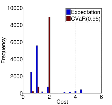
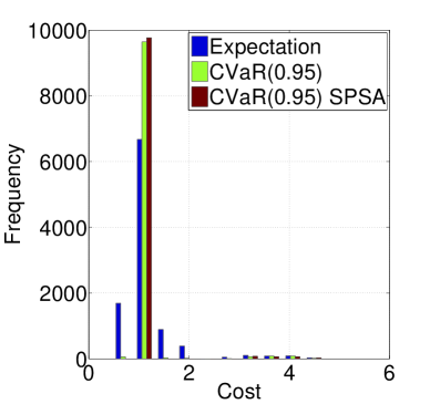
Figure 1: Cost distributions for the policies learned by the CVaR-constrained and risk-neutral policy gradient and actor-critic algorithms. The left figure corresponds to the PG methods and the right figure corresponds to the AC algorithms.

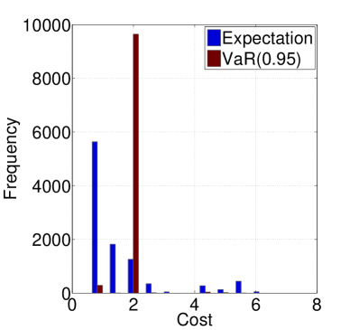
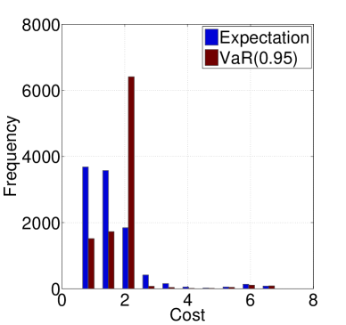
Figure 2: Cost distributions for the policies learned by the chance-constrained and risk-neutral policy gradient and actor-critic algorithms. The left figure corresponds to the PG methods and the right figure corresponds to the AC algorithms.

	$\mathbb{E}\big{(}{\color[rgb]{0,0,0}\mathcal{G}}^{\theta}(x^{0})\big{)}$	$\sigma\big{(}{\color[rgb]{0,0,0}\mathcal{G}}^{\theta}(x^{0})\big{)}$	$\text{CVaR}\big{(}{\color[rgb]{0,0,0}\mathcal{G}}^{\theta}(x^{0})\big{)}$	$\text{VaR}\big{(}{\color[rgb]{0,0,0}\mathcal{G}}^{\theta}(x^{0})\big{)}$
PG	1.177	1.065	4.464	4.005
PG-CVaR	1.997	0.060	2.000	2.000
PG-CC	1.994	0.121	2.058	2.000
AC	1.113	0.607	3.331	3.220
AC-CVaR-SPSA	1.326	0.322	2.145	1.283
AC-CVaR	1.343	0.346	2.208	1.290
AC-VaR	1.817	0.753	4.006	2.300

Table 1: Performance comparison of the policies learned by the risk-constrained and risk-neutral algorithms. In this table $\sigma\big{(}{\color[rgb]{0,0,0}\mathcal{G}}^{\theta}(x^{0})\big{)}$ stands for the standard deviation of the total cost.

6.2 A Personalized Ad-Recommendation System

Many companies such as banks and retailers use user-specific targeting of advertisements to attract more customers and increase their revenue. When a user requests a webpage that contains a box for an advertisement, the system should decide which advertisement (among those in the current campaign) to show to this particular user based on a vector containing all her features, often collected by a cookie. Our goal here is to generate a strategy that for each user of the website selects an ad that when it is presented to her has the highest probability to be clicked on. These days, almost all the industrial personalized ad recommendation systems use supervised learning or contextual bandits algorithms. These methods are based on the i.i.d. assumption of the visits (to the website) and do not discriminate between a visit and a visitor, i.e., each visit is considered as a new visitor that has been sampled i.i.d. from the population of the visitors. As a result, these algorithms are myopic and do not try to optimize for the long-term performance. Despite their success, these methods seem to be insufficient as users establish longer-term relationship with the websites they visit, i.e., the ad recommendation systems should deal with more and more returning visitors. The increase in returning visitors violates (more) the main assumption underlying the supervised learning and bandit algorithms, i.e., there is no difference between a visit and a visitor, and thus, shows the need for a new class of solutions.

The reinforcement learning (RL) algorithms that have been designed to optimize the long-term performance of the system (expected sum of rewards/costs) seem to be suitable candidates for ad recommendation systems (Shani et al., 2002). The nature of these algorithms allows them to take into account all the available knowledge about the user at the current visit, and then selects an offer to maximize the total number of times she will click over multiple visits, also known as the user’s life-time value (LTV). Unlike myopic approaches, RL algorithms differentiate between a visit and a visitor, and consider all the visits of a user (in chronological order) as a trajectory generated by her. In this approach, while the visitors are i.i.d. samples from the population of the users, their visits are not. This long-term approach to the ad recommendation problem allows us to make decisions that are not usually possible with myopic techniques, such as to propose an offer to a user that might be a loss to the company in the short term, but has the effect that makes the user engaged with the website/company and brings her back to spend more money in the future.

For our second case study, we use an Adobe personalized ad-recommendation (Theocharous and Hallak, 2013) simulator that has been trained based on real data captured with permission from the website of a Fortune 50 company that receives hundreds of visitors per day. The simulator produces a vector of $31$ real-valued features that provide a compressed representation of all of the available information about a user. The advertisements are clustered into four high-level classes that the agent must select between. After the agent selects an advertisement, the user either clicks (reward of $+1$) or does not click (reward of $0$) and the feature vector describing the user is updated. In this case, we test our algorithm by maximizing the customers’ life-time value in $15$ time steps subject to a bounded tail risk.

Instead of using the cost-minimization framework from the main paper, by defining the return random variable (under a fixed policy $\theta$) $\mathcal{R}^{\theta}(x^{0})$ as the (discounted) total number of clicks along a user’s trajectory, here we formulate the personalized ad-recommendation problem as a return maximization problem where the tail risk corresponds to the worst case return distribution:

$$\max_{\theta}\mathbb{E}\left[\mathcal{R}^{\theta}(x^{0})\right]\quad\quad\text{{\color[rgb]{0,0,0}subject to}}\quad\quad{\color[rgb]{0,0,0}\text{CVaR}_{1-\alpha}\big{(}-\mathcal{R}^{\theta}(x^{0})\big{)}\leq\beta}.$$ (38)

We set the parameters of the MDP as $T=15$ and $\gamma=0.98$, the confidence level and constraint threshold as $\alpha=0.05$ and $\beta=-0.12$, the number of sample trajectories $N$ to $1,000,000$, and the parameter bounds as $\lambda_{\max}=5,000$ and $\Theta=[-60,60]^{\kappa_{1}}$, where the dimension of the basis functions is $\kappa_{1}=4096$. Similar to the optimal stopping problem, we implement both the trajectory based algorithm (PG, PG-CVaR) and the actor-critic algorithms (AC, AC-CVaR) for risk-neutral and risk sensitive optimal control. Here we used the $3^{\text{rd}}$ order Fourier basis with cross-products in Konidaris et al. (2011) as features and search over the family of Boltzmann policies. We compared the performance of PG-CVaR and AC-CVaR, our risk-constrained policy gradient (Algorithm 1) and actor-critic (Algorithms 2) algorithms, with their risk-neutral counterparts (PG and AC). Figure 3 shows the distribution of the discounted cumulative return $\mathcal{R}^{\theta}(x^{0})$ for the policy $\theta$ learned by each of these algorithms. The results indicate that the risk-constrained algorithms yield a lower expected reward, but have higher left tail (worst-case) reward distributions. Table 2 summarizes the findings of this experiment.

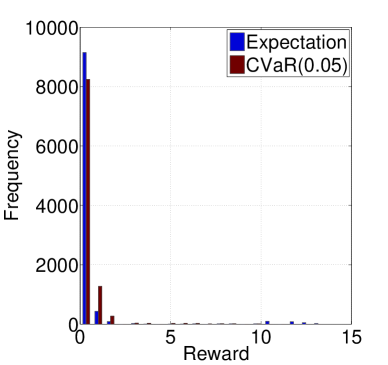
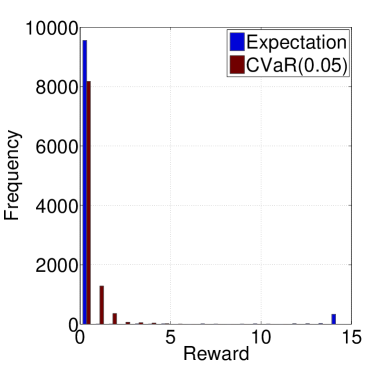
Figure 3: Reward distributions for the policies learned by the CVaR-constrained and risk-neutral policy gradient and actor-critic algorithms. The left figure corresponds to the PG methods and the right figure corresponds to the AC algorithms.

	$\mathbb{E}\big{(}\mathcal{R}^{\theta}(x^{0})\big{)}$	$\sigma\big{(}\mathcal{R}^{\theta}(x^{0})\big{)}$	$\text{CVaR}\big{(}\mathcal{R}^{\theta}(x^{0})\big{)}$	$\text{VaR}\big{(}\mathcal{R}^{\theta}(x^{0})\big{)}$
PG	0.396	1.898	0.037	1.000
PG-CVaR	0.287	0.914	0.126	1.795
AC	0.581	2.778	0	0
AC-CVaR	0.253	0.634	0.137	1.890

Table 2: Performance comparison of the policies learned by the CVaR-constrained and risk-neutral algorithms. In this table $\sigma\big{(}\mathcal{R}^{\theta}(x^{0})\big{)}$ stands for the standard deviation of the total reward.

7 Conclusions and Future Work

We proposed novel policy gradient and actor-critic algorithms for CVaR-constrained and chance-constrained optimization in MDPs, and proved their convergence. Using an optimal stopping problem and a personalized ad-recommendation problem, we showed that our algorithms resulted in policies whose cost distributions have lower right-tail compared to their risk-neutral counterparts. This is important for a risk-averse decision-maker, especially if the right-tail contains catastrophic costs. Future work includes: 1) Providing convergence proofs for our AC algorithms when the samples are generated by following the policy and not from its discounted occupation measure , 2) Using importance sampling methods (Bardou et al., 2009; Tamar et al., 2015) to improve gradient estimates in the right-tail of the cost distribution (worst-case events that are observed with low probability), and 3) Applying the algorithms presented in this paper to a variety of applications ranging from operations research to robotics and finance.

Acknowledgments

We would like to thank Csaba Szepesvari for his comments that helped us with the derivation of the algorithms, Georgios Theocharous for sharing his ad-recommendation simulator with us, and Philip Thomas for helping us with the experiments with the simulator. We would also like to thank the reviewers for their very helpful comments and suggestions, which helped us to significantly improve the paper. Y-L. Chow is partially supported by The Croucher Foundation doctoral scholarship. L. Janson was partially supported by NIH training grant T32GM096982. M. Pavone was partially supported by the Office of Naval Research, Science of Autonomy Program, under Contract N00014-15-1-2673.

A Convergence of Policy Gradient Methods

A.1 Computing the Gradients

i) $\nabla_{\theta}L(\nu,\theta,\lambda)$: Gradient of $L(\nu,\theta,\lambda)$ w.r.t. $\theta$ By expanding the expectations in the definition of the objective function $L(\nu,\theta,\lambda)$ in (5), we obtain

$$L(\nu,\theta,\lambda)=\sum_{\xi}\mathbb{P}_{\theta}(\xi){\color[rgb]{0,0,0}\mathcal{G}}(\xi)+\lambda\nu+\frac{\lambda}{1-\alpha}\sum_{\xi}\mathbb{P}_{\theta}(\xi)\big{(}{\color[rgb]{0,0,0}\mathcal{J}}(\xi)-\nu\big{)}^{+}-\lambda\beta.$$

By taking the gradient with respect to $\theta$, we have

$$\nabla_{\theta}L(\nu,\theta,\lambda)=\sum_{\xi}\nabla_{\theta}\mathbb{P}_{\theta}(\xi){\color[rgb]{0,0,0}\mathcal{G}}(\xi)+\frac{\lambda}{1-\alpha}\sum_{\xi}\nabla_{\theta}\mathbb{P}_{\theta}(\xi)\big{(}{\color[rgb]{0,0,0}\mathcal{J}}(\xi)-\nu\big{)}^{+}.$$

This gradient can be rewritten as

$$\nabla_{\theta}L(\nu,\theta,\lambda)=\sum_{\xi:{\color[rgb]{0,0,0}\mathbb{P}_{\theta}(\xi)\neq 0}}\mathbb{P}_{\theta}(\xi)\cdot\nabla_{\theta}\log\mathbb{P}_{\theta}(\xi)\left({\color[rgb]{0,0,0}\mathcal{G}}(\xi)+\frac{\lambda}{1-\alpha}\big{(}{\color[rgb]{0,0,0}\mathcal{J}}(\xi)-\nu\big{)}\mathbf{1}\big{\{}{\color[rgb]{0,0,0}\mathcal{J}}(\xi)\geq\nu\big{\}}\right),$$ (39)

where in the case of $\mathbb{P}_{\theta}(\xi)\neq 0$, the term $\nabla_{\theta}\log\mathbb{P}_{\theta}(\xi)$ is given by:

$$\begin{split}\nabla_{\theta}\log\mathbb{P}_{\theta}(\xi)=&\nabla_{\theta}\left\{\sum_{k=0}^{T-1}\log P(x_{k+1}|x_{k},a_{k})+\log\mu(a_{k}|x_{k};\theta)+\log\mathbf{1}\{x_{0}=x^{0}\}\right\}\\ =&\sum_{k=0}^{T-1}\nabla_{\theta}\log\mu(a_{k}|x_{k};\theta)\\ =&\sum_{k=0}^{T-1}\frac{1}{\mu(a_{k}|x_{k};\theta)}\nabla_{\theta}\mu(a_{k}|x_{k};\theta).\end{split}$$

ii) $\partial_{\nu}L(\nu,\theta,\lambda)$: Sub-differential of $L(\nu,\theta,\lambda)$ w.r.t. $\nu$ From the definition of $L(\nu,\theta,\lambda)$, we can easily see that $L(\nu,\theta,\lambda)$ is a convex function in $\nu$ for any fixed $\theta\in\Theta$. Note that for every fixed $\nu$ and any $\nu^{\prime}$, we have

$$\big{(}{\color[rgb]{0,0,0}\mathcal{J}}(\xi)-\nu^{\prime}\big{)}^{+}-\big{(}{\color[rgb]{0,0,0}\mathcal{J}}(\xi)-\nu\big{)}^{+}\geq g\cdot(\nu^{\prime}-\nu),$$

where $g$ is any element in the set of sub-derivatives:

$$g\in\partial_{\nu}\big{(}{\color[rgb]{0,0,0}\mathcal{J}}(\xi)-\nu\big{)}^{+}:=\begin{cases}-1&\text{if $\nu<{\color[rgb]{0,0,0}\mathcal{J}}(\xi)$},\\ -q:q\in[0,1]&\text{if $\nu={\color[rgb]{0,0,0}\mathcal{J}}(\xi)$},\\ 0&\text{otherwise}.\end{cases}$$

Since $L(\nu,\theta,\lambda)$ is finite-valued for any $\nu\in$, by the additive rule of sub-derivatives, we have

$$\partial_{\nu}L(\nu,\theta,\lambda)=\left\{-\frac{\lambda}{1-\alpha}\sum_{\xi}\mathbb{P}_{\theta}(\xi)\mathbf{1}\big{\{}{\color[rgb]{0,0,0}\mathcal{J}}(\xi)>\nu\big{\}}-\frac{\lambda q}{1-\alpha}\sum_{\xi}\mathbb{P}_{\theta}(\xi)\mathbf{1}\big{\{}{\color[rgb]{0,0,0}\mathcal{J}}(\xi)=\nu\big{\}}+\lambda\mid q\in[0,1]\right\}.$$ (40)

In particular for $q=1$, we may write the sub-gradient of $L(\nu,\theta,\lambda)$ w.r.t. $\nu$ as

$$\partial_{\nu}L(\nu,\theta,\lambda)|_{q=0}=\lambda-\frac{\lambda}{1-\alpha}\sum_{\xi}\mathbb{P}_{\theta}(\xi)\cdot\mathbf{1}\big{\{}{\color[rgb]{0,0,0}\mathcal{J}}(\xi)\geq\nu\big{\}}$$

or

$$\lambda-\frac{\lambda}{1-\alpha}\sum_{\xi}\mathbb{P}_{\theta}(\xi)\cdot\mathbf{1}\big{\{}{\color[rgb]{0,0,0}\mathcal{J}}(\xi)\geq\nu\big{\}}\in\partial_{\nu}L(\nu,\theta,\lambda).$$

iii) $\nabla_{\lambda}L(\nu,\theta,\lambda)$: Gradient of $L(\nu,\theta,\lambda)$ w.r.t. $\lambda$ Since $L(\nu,\theta,\lambda)$ is a linear function in $\lambda$, one can express the gradient of $L(\nu,\theta,\lambda)$ w.r.t. $\lambda$ as follows:

$$\nabla_{\lambda}L(\nu,\theta,\lambda)=\nu-\beta+\frac{1}{1-\alpha}\sum_{\xi}\mathbb{P}_{\theta}(\xi)\cdot\big{(}{\color[rgb]{0,0,0}\mathcal{J}}(\xi)-\nu\big{)}\mathbf{1}\big{\{}{\color[rgb]{0,0,0}\mathcal{J}}(\xi)\geq\nu\big{\}}.$$ (41)

A.2 Proof of Convergence of the Policy Gradient Algorithm

In this section, we prove the convergence of the policy gradient algorithm (Algorithm 1). Before going through the details of the convergence proof, a high level overview of the proof technique is given as follows.

1. First, by convergence properties of multi-time scale discrete stochastic approximation algorithms, we show that each update $(\nu_{k},\theta_{k},\lambda_{k})$ converges almost surely to a stationary point $(\nu^{\ast},\theta^{*},\lambda^{*})$ of the corresponding continuous time system. In particular, by adopting the step-size rules defined in Assumption 6, we show that the convergence rate of $\nu$ is fastest, followed by the convergence rate of $\theta$, while the convergence rate of $\lambda$ is the slowest among the set of parameters.

2. By using Lyapunov analysis, we show that the continuous time system is locally asymptotically stable at the stationary point $(\nu^{\ast},\theta^{*},\lambda^{*})$.

3. Since the Lyapunov function used in the above analysis is the Lagrangian function $L(\nu,\theta,\lambda)$, we conclude that the stationary point $(\nu^{\ast},\theta^{*},\lambda^{*})$ is a local saddle point. Finally by the local saddle point theorem, we deduce that $\theta^{*}$ is a locally optimal solution for the CVaR-constrained MDP problem.

This convergence proof procedure is standard for stochastic approximation algorithms, see (Bhatnagar et al., 2009; Bhatnagar and Lakshmanan, 2012) for further references.

Since $\nu$ converges on the faster timescale than $\theta$ and $\lambda$, the $\nu$-update can be rewritten by assuming $(\theta,\lambda)$ as invariant quantities, i.e.,

$$\nu_{k+1}=\Gamma_{\mathcal{N}}\bigg{[}\nu_{k}-\zeta_{3}(k)\bigg{(}\lambda-\frac{\lambda}{(1-\alpha)N}\sum_{j=1}^{N}\mathbf{1}\big{\{}{\color[rgb]{0,0,0}\mathcal{J}}(\xi_{j,k})\geq\nu_{k}\big{\}}\bigg{)}\bigg{]}.$$ (42)

Consider the continuous time dynamics of $\nu$ defined using differential inclusion

$$\dot{\nu}\in\Upsilon_{\nu}\left[-g(\nu)\right],\quad\quad\forall g(\nu)\in\partial_{\nu}L(\nu,\theta,\lambda),$$ (43)

where

$$\Upsilon_{\nu}[K(\nu)]:=\lim_{0<\eta\rightarrow 0}\frac{\Gamma_{\mathcal{N}}(\nu+\eta K(\nu))-\Gamma_{\mathcal{N}}(\nu)}{\eta}.$$

Here $\Upsilon_{\nu}[K(\nu)]$ is the left directional derivative of the function $\Gamma_{\mathcal{N}}(\nu)$ in the direction of $K(\nu)$. By using the left directional derivative $\Upsilon_{\nu}\left[-g(\nu)\right]$ in the sub-gradient descent algorithm for $\nu$, the gradient will point in the descent direction along the boundary of $\nu$ whenever the $\nu$-update hits its boundary.

Furthermore, since $\nu$ converges on a faster timescale than $\theta$, and $\lambda$ is on the slowest time-scale, the $\theta$-update can be rewritten using the converged $\nu^{*}(\theta)$, assuming $\lambda$ as an invariant quantity, i.e.,

$$\begin{split}\theta_{k+1}=&\Gamma_{\Theta}\bigg{[}\theta_{k}-\zeta_{2}(k)\bigg{(}\frac{1}{N}\sum_{j=1}^{N}\nabla_{\theta}\log\mathbb{P}_{\theta}(\xi_{j,k})|_{\theta=\theta_{k}}{\color[rgb]{0,0,0}\mathcal{G}}(\xi_{j,k})\\ &\hskip 52.39618pt+\frac{\lambda}{(1-\alpha)N}\sum_{j=1}^{N}\nabla_{\theta}\log\mathbb{P}_{\theta}(\xi_{j,k})|_{\theta=\theta_{k}}\big{(}{\color[rgb]{0,0,0}\mathcal{J}}(\xi_{j,k})-\nu\big{)}\mathbf{1}\big{\{}{\color[rgb]{0,0,0}\mathcal{J}}(\xi_{j,k})\geq\nu^{*}(\theta_{k})\big{\}}\bigg{)}\bigg{]}.\end{split}$$

Consider the continuous time dynamics of $\theta\in\Theta$:

$$\dot{\theta}=\Upsilon_{\theta}\left[-\nabla_{\theta}L(\nu,\theta,\lambda)\right]|_{\nu=\nu^{*}(\theta)},$$ (44)

where

$$\Upsilon_{\theta}[K(\theta)]:=\lim_{0<\eta\rightarrow 0}\frac{\Gamma_{\Theta}(\theta+\eta K(\theta))-\Gamma_{\Theta}(\theta)}{\eta}.$$

Similar to the analysis of $\nu$, $\Upsilon_{\theta}[K(\theta)]$ is the left directional derivative of the function $\Gamma_{\Theta}(\theta)$ in the direction of $K(\theta)$. By using the left directional derivative $\Upsilon_{\theta}\left[-\nabla_{\theta}L(\nu,\theta,\lambda)\right]$ in the gradient descent algorithm for $\theta$, the gradient will point in the descent direction along the boundary of $\Theta$ whenever the $\theta$-update hits its boundary.

Finally, since the $\lambda$-update converges in the slowest time-scale, the $\lambda$-update can be rewritten using the converged $\theta^{*}(\lambda)$ and $\nu^{*}(\lambda)$, i.e.,

$$\lambda_{k+1}=\Gamma_{\Lambda}\left(\lambda_{k}+\zeta_{1}(k)\bigg{(}\nu^{*}(\lambda_{k})+\frac{1}{1-\alpha}\frac{1}{N}\sum_{j=1}^{N}\big{(}{\color[rgb]{0,0,0}\mathcal{J}}(\xi_{j,k})-\nu^{*}(\lambda_{k})\big{)}^{+}-\beta\bigg{)}\right).$$ (45)

Consider the continuous time system

$$\dot{\lambda}(t)=\Upsilon_{\lambda}\left[\nabla_{\lambda}L(\nu,\theta,\lambda)\bigg{|}_{\theta=\theta^{*}(\lambda),\nu=\nu^{*}(\lambda)}\right],\quad\quad\lambda(t)\geq 0,$$ (46)

where

$$\Upsilon_{\lambda}[K(\lambda)]:=\lim_{0<\eta\rightarrow 0}\frac{\Gamma_{\Lambda}\big{(}\lambda+\eta K(\lambda)\big{)}-\Gamma_{\Lambda}(\lambda)}{\eta}.$$

Again, similar to the analysis of $(\nu,\theta)$, $\Upsilon_{\lambda}[K(\lambda)]$ is the left directional derivative of the function $\Gamma_{\Lambda}(\lambda)$ in the direction of $K(\lambda)$. By using the left directional derivative $\Upsilon_{\lambda}\left[\nabla_{\lambda}L(\nu,\theta,\lambda)\right]$ in the gradient ascent algorithm for $\lambda$, the gradient will point in the ascent direction along the boundary of $[0,\lambda_{\max}]$ whenever the $\lambda$-update hits its boundary.

Define

$$L^{*}(\lambda)=L(\nu^{\ast}(\lambda),\theta^{\ast}(\lambda),\lambda),$$

for $\lambda\geq 0$ where $(\theta^{\ast}(\lambda),\nu^{\ast}(\lambda))\in\Theta\times[-\frac{D_{\max}}{1-\gamma},\frac{D_{\max}}{1-\gamma}]$ is a local minimum of $L(\nu,\theta,\lambda)$ for fixed $\lambda\geq 0$, i.e., $L(\nu,\theta,\lambda)\geq L(\nu^{\ast}(\lambda),\theta^{\ast}(\lambda),\lambda)$ for any $(\theta,\nu)\in\Theta\times[-\frac{D_{\max}}{1-\gamma},\frac{D_{\max}}{1-\gamma}]\cap\mathcal{B}_{(\theta^{\ast}(\lambda),\nu^{\ast}(\lambda))}(r)$ for some $r>0$.

Next, we want to show that the ODE (46) is actually a gradient ascent of the Lagrangian function using the envelope theorem from mathematical economics (Milgrom and Segal, 2002). The envelope theorem describes sufficient conditions for the derivative of $L^{*}$ with respect to $\lambda$ to equal the partial derivative of the objective function $L$ with respect to $\lambda$, holding $(\theta,\nu)$ at its local optimum $(\theta,\nu)=(\theta^{\ast}(\lambda),\nu^{\ast}(\lambda))$. We will show that $\nabla_{\lambda}L^{\ast}(\lambda)$ coincides with $\nabla_{\lambda}L(\nu,\theta,\lambda)|_{\theta=\theta^{\ast}(\lambda),\nu=\nu^{\ast}(\lambda)}$ as follows.

Theorem 16

The value function $L^{*}$ is absolutely continuous. Furthermore,

$$L^{*}(\lambda)=L^{*}(0)+\int_{0}^{\lambda}\nabla_{\lambda^{\prime}}L(\nu,\theta,\lambda^{\prime})\Big{|}_{\theta=\theta^{*}(s),\nu=\nu^{*}(s),\lambda^{\prime}=s}ds,\,\,\lambda\geq 0.$$ (47)

Proof. The proof follows from analogous arguments to Lemma 4.3 in Borkar (2005). From the definition of $L^{*}$, observe that for any $\lambda^{\prime},\lambda^{\prime\prime}\geq 0$ with $\lambda^{\prime}<\lambda^{\prime\prime}$,

$$\begin{split}|L^{*}(\lambda^{\prime\prime})-L^{*}(\lambda^{\prime})|\leq&\sup_{\theta\in\Theta,\nu\in[-\frac{D_{\max}}{1-\gamma},\frac{D_{\max}}{1-\gamma}]}|L(\nu,\theta,\lambda^{\prime\prime})-L(\nu,\theta,\lambda^{\prime})|\\ =&\sup_{\theta\in\Theta,\nu\in[-\frac{D_{\max}}{1-\gamma},\frac{D_{\max}}{1-\gamma}]}\left|\int_{\lambda^{\prime}}^{\lambda^{\prime\prime}}\nabla_{\lambda}L(\nu,\theta,s)ds\right|\\ \leq&\int_{\lambda^{\prime}}^{\lambda^{\prime\prime}}\sup_{\theta\in\Theta,\nu\in[\frac{-D_{\max}}{1-\gamma},\frac{D_{\max}}{1-\gamma}]}\left|\nabla_{\lambda}L(\nu,\theta,s)\right|ds\leq\frac{3D_{\max}}{(1-\alpha)(1-\gamma)}(\lambda^{\prime\prime}-\lambda^{\prime}).\end{split}$$

This implies that $L^{*}$ is absolutely continuous. Therefore, $L^{*}$ is continuous everywhere and differentiable almost everywhere.

By the Milgrom–Segal envelope theorem in mathematical economics (Theorem 1 of Milgrom and Segal (2002)), one concludes that the derivative of $L^{*}(\lambda)$ coincides with the derivative of $L(\nu,\theta,\lambda)$ at the point of differentiability $\lambda$ and $\theta=\theta^{*}(\lambda)$, $\nu=\nu^{*}(\lambda)$. Also since $L^{*}$ is absolutely continuous, the limit of $(L^{*}(\lambda)-L^{*}(\lambda^{\prime}))/(\lambda-\lambda^{\prime})$ at $\lambda\uparrow\lambda^{\prime}$ (or $\lambda\downarrow\lambda^{\prime}$) coincides with the lower/upper directional derivatives if $\lambda^{\prime}$ is a point of non-differentiability. Thus, there is only a countable number of non-differentiable points in $L^{*}$ and the set of non-differentiable points of $L^{*}$ has measure zero. Therefore, expression (47) holds and one concludes that $\nabla_{\lambda}L^{\ast}(\lambda)$ coincides with $\nabla_{\lambda}L(\nu,\theta,\lambda)|_{\theta=\theta^{*}(\lambda),\nu=\nu^{*}(\lambda)}$. $\blacksquare$

Before getting into the main result, we have the following technical proposition whose proof directly follows from the definition of $\log\mathbb{P}_{\theta}(\xi)$ and Assumption 3 that $\nabla_{\theta}\mu(a_{k}|x_{k};\theta)$ is Lipschitz in $\theta$.

Proposition 17

$\nabla_{\theta}L(\nu,\theta,\lambda)$ is Lipschitz in $\theta$.

Proof. Recall that

$$\nabla_{\theta}L(\nu,\theta,\lambda)=\sum_{\xi}\mathbb{P}_{\theta}(\xi)\cdot\nabla_{\theta}\log\mathbb{P}_{\theta}(\xi)\left({\color[rgb]{0,0,0}\mathcal{G}}(\xi)+\frac{\lambda}{1-\alpha}\big{(}{\color[rgb]{0,0,0}\mathcal{J}}(\xi)-\nu\big{)}\mathbf{1}\big{\{}{\color[rgb]{0,0,0}\mathcal{J}}(\xi)\geq\nu\big{\}}\right)$$

and $\nabla_{\theta}\log\mathbb{P}_{\theta}(\xi)=\sum_{k=0}^{T-1}\nabla_{\theta}\mu(a_{k}|x_{k};\theta)/\mu(a_{k}|x_{k};\theta)$ whenever $\mu(a_{k}|x_{k};\theta)\in(0,1]$. Now Assumption (A1) implies that $\nabla_{\theta}\mu(a_{k}|x_{k};\theta)$ is a Lipschitz function in $\theta$ for any $a\in\mathcal{A}$ and $k\in\{0,\ldots,T-1\}$ and $\mu(a_{k}|x_{k};\theta)$ is differentiable in $\theta$. Therefore, by recalling that

$$\mathbb{P}_{\theta}(\xi)=\prod_{k=0}^{T-1}P(x_{k+1}|x_{k},a_{k})\mu(a_{k}|x_{k};\theta)\mathbf{1}\{x_{0}=x^{0}\}$$

and by combining these arguments and noting that the sum of products of Lipschitz functions is Lipschitz, one concludes that $\nabla_{\theta}L(\nu,\theta,\lambda)$ is Lipschitz in $\theta$. $\blacksquare$

Remark 18

The fact that $\nabla_{\theta}L(\nu,\theta,\lambda)$ is Lipschitz in $\theta$ implies that

$$\|\nabla_{\theta}L(\nu,\theta,\lambda)\|^{2}\leq 2(\|\nabla_{\theta}L(\nu,\theta_{0},\lambda)\|+\|\theta_{0}\|)^{2}+2\|\theta\|^{2}$$

which further implies that

$$\|\nabla_{\theta}L(\nu,\theta,\lambda)\|^{2}\leq K_{1}(1+\|\theta\|^{2}).$$

for $K_{1}=2\max(1,(\|\nabla_{\theta}L(\nu,\theta_{0},\lambda)\|+\|\theta_{0}\|)^{2})>0$. Similarly, the fact that $\nabla_{\theta}\log\mathbb{P}_{\theta}(\xi)$ is Lipschitz implies that

$$\|\nabla_{\theta}\log\mathbb{P}_{\theta}(\xi)\|^{2}\leq K_{2}(\xi)(1+\|\theta\|^{2})$$

for a positive random variable $K_{2}(\xi)$. Furthermore, since $T<\infty$ w.p. $1$, $\mu(a_{k}|x_{k};\theta)\in(0,1]$ and $\nabla_{\theta}\mu(a_{k}|x_{k};\theta)$ is Lipschitz for any $k<T$, $K_{2}(\xi)<\infty$ w.p. $1$.

Remark 19

For any given $\theta\in\Theta$, $\lambda\geq 0$, and $g(\nu)\in\partial_{\nu}L(\nu,\theta,\lambda)$, we have

$$|g(\nu)|\leq 3\lambda(1+|\nu|)/(1-\alpha).$$ (48)

To see this, recall that the set of $g(\nu)\in\partial_{\nu}L(\nu,\theta,\lambda)$ can be parameterized by $q\in[0,1]$ as

$$g(\nu;q)=-\frac{\lambda}{(1-\alpha)}\sum_{\xi}\mathbb{P}_{\theta}(\xi)\mathbf{1}\left\{{\color[rgb]{0,0,0}\mathcal{J}}(\xi)>\nu\right\}-\frac{\lambda q}{1-\alpha}\sum_{\xi}\mathbb{P}_{\theta}(\xi)\mathbf{1}\left\{{\color[rgb]{0,0,0}\mathcal{J}}(\xi)=\nu\right\}+\lambda.$$

It is obvious that $\left|\mathbf{1}\left\{{\color[rgb]{0,0,0}\mathcal{J}}(\xi)=\nu\right\}\right|,\left|\mathbf{1}\left\{{\color[rgb]{0,0,0}\mathcal{J}}(\xi)>\nu\right\}\right|\leq 1+|\nu|$. Thus, $\left|\sum_{\xi}\mathbb{P}_{\theta}(\xi)\mathbf{1}\left\{{\color[rgb]{0,0,0}\mathcal{J}}(\xi)>\nu\right\}\right|\leq\sup_{\xi}\left|\mathbf{1}\left\{{\color[rgb]{0,0,0}\mathcal{J}}(\xi)>\nu\right\}\right|\leq 1+|\nu|$, and $\left|\sum_{\xi}\mathbb{P}_{\theta}(\xi)\mathbf{1}\left\{{\color[rgb]{0,0,0}\mathcal{J}}(\xi)=\nu\right\}\right|\leq 1+|\nu|$. Recalling that $0<(1-q),\,(1-\alpha)<1$, these arguments imply the claim of (48).

We are now in a position to prove the convergence analysis of Theorem 7.

Proof. [Proof of Theorem 7] We split the proof into the following four steps:

Step 1 (Convergence of $\nu$-update)

Since $\nu$ converges on a faster time scale than $\theta$ and $\lambda$, according to Lemma 1 in Chapter 6 of Borkar (2008), one can analyze the convergence properties of $\nu$ in the following update rule for arbitrary quantities of $\theta$ and $\lambda$ (i.e., here we have $\theta=\theta_{k}$ and $\lambda=\lambda_{k}$):

$$\nu_{k+1}=\Gamma_{\mathcal{N}}\left(\nu_{k}+\zeta_{3}(k)\left(\frac{\lambda}{(1-\alpha)N}\sum_{j=1}^{N}\mathbf{1}\big{\{}{\color[rgb]{0,0,0}\mathcal{J}}(\xi_{j,k})\geq\nu_{k}\big{\}}-\lambda+\delta\nu_{k+1}\right)\right),$$ (49)

and the Martingale difference term with respect to $\nu$ is given by

$$\delta\nu_{k+1}=\frac{\lambda}{1-\alpha}\left(-\frac{1}{N}\sum_{j=1}^{N}\mathbf{1}\big{\{}{\color[rgb]{0,0,0}\mathcal{J}}(\xi_{j,k})\geq\nu_{k}\big{\}}+\sum_{\xi}\mathbb{P}_{\theta}(\xi)\mathbf{1}\{{\color[rgb]{0,0,0}\mathcal{J}}(\xi)\geq\nu_{k}\}\right).$$ (50)

First, one can show that $\delta\nu_{k+1}$ is square integrable, i.e.,

$$\mathbb{E}[\|\delta\nu_{k+1}\|^{2}\mid F_{\nu,k}]\leq 4\left(\frac{\lambda_{\max}}{1-\alpha}\right)^{2}$$

where $\mathcal{F}_{\nu,k}=\sigma\big{(}\nu_{m},\,\delta\nu_{m},\,m\leq k\big{)}$ is the filtration of $\nu_{k}$ generated by different independent trajectories.

Second, since the history trajectories are generated based on the sampling probability mass function $\mathbb{P}_{\theta}(\xi)$, expression (40) implies that $\mathbb{E}\left[\delta\nu_{k+1}\mid\mathcal{F}_{\nu,k}\right]=0$. Therefore, the $\nu$-update is a stochastic approximation of the ODE (43) with a Martingale difference error term, i.e.,

$$\frac{\lambda}{1-\alpha}\sum_{\xi}\mathbb{P}_{\theta}(\xi)\mathbf{1}\{{\color[rgb]{0,0,0}\mathcal{J}}(\xi)\geq\nu_{k}\}-\lambda\in-\partial_{\nu}L(\nu,\theta,\lambda)|_{\nu=\nu_{k}}.$$

Then one can invoke Corollary 4 in Chapter 5 of Borkar (2008) (stochastic approximation theory for non-differentiable systems) to show that the sequence $\{\nu_{k}\},\;\nu_{k}\in[-\frac{D_{\max}}{1-\gamma},\frac{D_{\max}}{1-\gamma}]$ converges almost surely to a fixed point $\nu^{*}\in[-\frac{D_{\max}}{1-\gamma},\frac{D_{\max}}{1-\gamma}]$ of the differential inclusion (43), where

$$\nu^{\ast}\in N_{c}:=\left\{\nu\in\left[-\frac{D_{\max}}{1-\gamma},\frac{D_{\max}}{1-\gamma}\right]:\Upsilon_{\nu}[-g(\nu)]=0,\,g(\nu)\in\partial_{\nu}L(\nu,\theta,\lambda)\right\}.$$

To justify the assumptions of this corollary, 1) from Remark 19, the Lipschitz property is satisfied, i.e., $\sup_{g(\nu)\in\partial_{\nu}L(\nu,\theta,\lambda)}|g(\nu)|\leq 3\lambda(1+|\nu|)/(1-\alpha)$, 2) $[-\frac{D_{\max}}{1-\gamma},\frac{D_{\max}}{1-\gamma}]$ and $\partial_{\nu}L(\nu,\theta,\lambda)$ are convex compact sets by definition, which implies $\{(\nu,g(\nu))\mid g(\nu)\in\partial_{\nu}L(\nu,\theta,\lambda)\}$ is a closed set, and further implies $\partial_{\nu}L(\nu,\theta,\lambda)$ is an upper semi-continuous set valued mapping, 3) the step-size rule follows from Assumption 6, 4) the Martingale difference assumption follows from (50), and 5) $\nu_{k}\in[-\frac{D_{\max}}{1-\gamma},\frac{D_{\max}}{1-\gamma}]$, $\forall i$ implies that $\sup_{k}\|\nu_{k}\|<\infty$ almost surely.

Consider the ODE for $\nu\in$ in (43), we define the set-valued derivative of $L$ as follows:

$$D_{t}L(\nu,\theta,\lambda)=\big{\{}g(\nu)\Upsilon_{\nu}\big{[}-g(\nu)\big{]}\mid\forall g(\nu)\in\partial_{\nu}L(\nu,\theta,\lambda)\big{\}}.$$

One can conclude that

$$\max_{g(\nu)}D_{t}L(\nu,\theta,\lambda)=\max\big{\{}g(\nu)\Upsilon_{\nu}\big{[}-g(\nu)\big{]}\mid g(\nu)\in\partial_{\nu}L(\nu,\theta,\lambda)\big{\}}.$$

We now show that $\max_{g(\nu)}D_{t}L(\nu,\theta,\lambda)\leq 0$ and this quantity is non-zero if $\Upsilon_{\nu}\big{[}-g(\nu)\big{]}\neq 0$ for every $g(\nu)\in\partial_{\nu}L(\nu,\theta,\lambda)$ by considering three cases. To distinguish the latter two cases, we need to define,

$${\color[rgb]{0,0,0}\mathcal{J}}(\nu):=\left\{g(\nu)\in\partial L_{\nu}(\nu,\theta,\lambda)\Big{|}\,\forall\eta_{0}>0,\,\exists\eta\in(0,\eta_{0}]\text{ such that }\theta-\eta g(\nu)\not\in\left[-\frac{D_{\max}}{1-\gamma},\frac{D_{\max}}{1-\gamma}\right]\right\}.$$

Case 1: $\nu\in(-\frac{D_{\max}}{1-\gamma},\frac{D_{\max}}{1-\gamma})$.
For every $g(\nu)\in\partial_{\nu}L(\nu,\theta,\lambda)$, there exists a sufficiently small $\eta_{0}>0$ such that $\nu-\eta_{0}g(\nu)\in[-\frac{D_{\max}}{1-\gamma},\frac{D_{\max}}{1-\gamma}]$ and

$$\Gamma_{\mathcal{N}}\big{(}\theta-\eta_{0}g(\nu)\big{)}-\theta=-\eta_{0}g(\nu).$$

Therefore, the definition of $\Upsilon_{\theta}[-g(\nu)]$ implies

$$\max_{g(\nu)}D_{t}L(\nu,\theta,\lambda)=\max\big{\{}-g^{2}(\nu)\mid g(\nu)\in\partial_{\nu}L(\nu,\theta,\lambda)\big{\}}\leq 0.$$ (51)

The maximum is attained because $\partial_{\nu}L(\nu,\theta,\lambda)$ is a convex compact set and $g(\nu)\Upsilon_{\nu}\big{[}-g(\nu)\big{]}$ is a continuous function. At the same time, we have $\max_{g(\nu)}D_{t}L(\nu,\theta,\lambda)<0$ whenever $0\not\in\partial_{\nu}L(\nu,\theta,\lambda)$.

Case 2: $\nu\in\{-\frac{D_{\max}}{1-\gamma},\frac{D_{\max}}{1-\gamma}\}$ and ${\color[rgb]{0,0,0}\mathcal{J}}(\nu)$ is empty.
The condition $\nu-\eta g(\nu)\in[-\frac{D_{\max}}{1-\gamma},\frac{D_{\max}}{1-\gamma}]$ implies that

$$\Upsilon_{\nu}\big{[}-g(\nu)\big{]}=-g(\nu).$$

Then we obtain

$$\max_{g(\nu)}D_{t}L(\nu,\theta,\lambda)=\max\big{\{}-g^{2}(\nu)\mid g(\nu)\in\partial_{\nu}L(\nu,\theta,\lambda)\big{\}}\leq 0.$$ (52)

Furthermore, we have $\max_{g(\nu)}D_{t}L(\nu,\theta,\lambda)<0$ whenever $0\not\in\partial_{\nu}L(\nu,\theta,\lambda)$.

Case 3: $\nu\in\{-\frac{D_{\max}}{1-\gamma},\frac{D_{\max}}{1-\gamma}\}$ and ${\color[rgb]{0,0,0}\color[rgb]{0,0,0}\mathcal{J}}(\nu)$ is nonempty.
First, consider any $g(\nu)\in{\color[rgb]{0,0,0}\mathcal{J}}(\nu)$. For any $\eta>0$, define $\nu_{\eta}:=\nu-\eta g(\nu)$. The above condition implies that when $0<\eta\rightarrow 0$, $\Gamma_{\mathcal{N}}\big{[}\nu_{\eta}\big{]}$ is the projection of $\nu_{\eta}$ to the tangent space of $[-\frac{D_{\max}}{1-\gamma},\frac{D_{\max}}{1-\gamma}]$. For any element $\hat{\nu}\in[-\frac{D_{\max}}{1-\gamma},\frac{D_{\max}}{1-\gamma}]$, since the set $\{\nu\in[-\frac{D_{\max}}{1-\gamma},\frac{D_{\max}}{1-\gamma}]:\|\nu-\nu_{\eta}\|_{2}\leq\|\hat{\nu}-\nu_{\eta}\|_{2}\}$ is compact, the projection of $\nu_{\eta}$ on $[-\frac{D_{\max}}{1-\gamma},\frac{D_{\max}}{1-\gamma}]$ exists. Furthermore, since $f(\nu):=\frac{1}{2}(\nu-\nu_{\eta})^{2}$ is a strongly convex function and $\nabla f(\nu)=\nu-\nu_{\eta}$, by the first order optimality condition, one obtains

$$\nabla f(\nu_{\eta}^{\ast})(\nu-\nu_{\eta}^{\ast})=(\nu_{\eta}^{\ast}-\nu_{\eta})(\nu-\nu_{\eta}^{\ast})\geq 0,\quad\forall\nu\in\left[-\frac{D_{\max}}{1-\gamma},\frac{D_{\max}}{1-\gamma}\right]$$

where $\nu_{\eta}^{\ast}$ is the unique projection of $\nu_{\eta}$ (the projection is unique because $f(\nu)$ is strongly convex and $[-\frac{D_{\max}}{1-\gamma},\frac{D_{\max}}{1-\gamma}]$ is a convex compact set). Since the projection (minimizer) is unique, the above equality holds if and only if $\nu=\nu_{\eta}^{\ast}$.

Therefore, for any $\nu\in[-\frac{D_{\max}}{1-\gamma},\frac{D_{\max}}{1-\gamma}]$ and $\eta>0$,

$$\begin{split}&g(\nu)\Upsilon_{\nu}\big{[}-g(\nu)\big{]}=g(\nu)\left(\lim_{0<\eta\rightarrow 0}\frac{\nu_{\eta}^{\ast}-\nu}{\eta}\right)\\ =&\left(\lim_{0<\eta\rightarrow 0}\frac{\nu-\nu_{\eta}}{\eta}\right)\left(\lim_{0<\eta\rightarrow 0}\frac{\nu_{\eta}^{\ast}-\nu}{\eta}\right)=\lim_{0<\eta\rightarrow 0}\frac{-\|\nu_{\eta}^{\ast}-\nu\|^{2}}{\eta^{2}}+\lim_{0<\eta\rightarrow 0}\big{(}\nu_{\eta}^{\ast}-\nu_{\eta}\big{)}\left(\frac{\nu_{\eta}^{\ast}-\nu}{\eta^{2}}\right)\leq 0.\end{split}$$

Second, for any $g(\nu)\in\partial_{\nu}L(\nu,\theta,\lambda)\cap{\color[rgb]{0,0,0}\mathcal{J}}(\nu)^{c}$, one obtains $\nu-\eta g(\nu)\in[-\frac{D_{\max}}{1-\gamma},\frac{D_{\max}}{1-\gamma}]$, for any $\eta\in(0,\eta_{0}]$ and some $\eta_{0}>0$. In this case, the arguments follow from case 2 and the following expression holds: $\Upsilon_{\nu}\big{[}-g(\nu)\big{]}=-g(\nu)$.

Combining these arguments, one concludes that

$$\small\begin{split}&\max_{g(\nu)}D_{t}L(\nu,\theta,\lambda)\\ \leq&\max\left\{\max\big{\{}g(\nu)\;\Upsilon_{\nu}\big{[}-g(\nu)\big{]}\mid g(\nu)\in{\color[rgb]{0,0,0}\mathcal{J}}(\nu)\big{\}},\max\big{\{}-g^{2}(\nu)\mid g(\nu)\in\partial_{\nu}L(\nu,\theta,\lambda)\cap{\color[rgb]{0,0,0}\mathcal{J}}(\nu)^{c}\big{\}}\right\}\leq 0.\end{split}$$ (53)

This quantity is non-zero whenever $0\not\in\{g(\nu)\;\Upsilon_{\nu}\big{[}-g(\nu)\big{]}\mid\forall g(\nu)\in\partial_{\nu}L(\nu,\theta,\lambda)\}$ (this is because, for any $g(\nu)\in\partial_{\nu}L(\nu,\theta,\lambda)\cap{\color[rgb]{0,0,0}\mathcal{J}}(\nu)^{c}$, one obtains $g(\nu)\;\Upsilon_{\nu}\big{[}-g(\nu)\big{]}=-g(\nu)^{2}$). Thus, by similar arguments one may conclude that $\max_{g(\nu)}D_{t}L(\nu,\theta,\lambda)\leq 0$ and it is non-zero if $\Upsilon_{\nu}\big{[}-g(\nu)\big{]}\neq 0$ for every $g(\nu)\in\partial_{\nu}L(\nu,\theta,\lambda)$.

Now for any given $\theta$ and $\lambda$, define the following Lyapunov function

$$\mathcal{L}_{\theta,\lambda}(\nu)=L(\nu,\theta,\lambda)-L(\nu^{*},\theta,\lambda)$$

where $\nu^{*}$ is a minimum point (for any given $(\theta,\lambda)$, $L$ is a convex function in $\nu$). Then $\mathcal{L}_{\theta,\lambda}(\nu)$ is a positive definite function, i.e., $\mathcal{L}_{\theta,\lambda}(\nu)\geq 0$. On the other hand, by the definition of a minimum point, one easily obtains $0\in\{g(\nu^{*})\;\Upsilon_{\nu}\big{[}-g(\nu^{*})\big{]}|_{\nu=\nu^{*}}\mid\forall g(\nu^{*})\in\partial_{\nu}L(\nu,\theta,\lambda)|_{\nu=\nu^{*}}\}$ which means that $\nu^{\ast}$ is also a stationary point, i.e., $\nu^{\ast}\in N_{c}$.

Note that $\max_{g(\nu)}D_{t}\mathcal{L}_{\theta,\lambda}(\nu)=\max_{g(\nu)}D_{t}L(\nu,\theta,\lambda)\leq 0$ and this quantity is non-zero if $\Upsilon_{\nu}\big{[}-g(\nu)\big{]}\neq 0$ for every $g(\nu)\in\partial_{\nu}L(\nu,\theta,\lambda)$. Therefore, by the Lyapunov theory for asymptotically stable differential inclusions (see Theorem 3.10 and Corollary 3.11 in Benaim et al. (2006), where the Lyapunov function $\mathcal{L}_{\theta,\lambda}(\nu)$ satisfies Hypothesis 3.1 and the property in (53) is equivalent to Hypothesis 3.9 in the reference), the above arguments imply that with any initial condition $\nu(0)$, the state trajectory $\nu(t)$ of (43) converges to $\nu^{\ast}$, i.e., $L(\nu^{\ast},\theta,\lambda)\leq L(\nu(t),\theta,\lambda)\leq L(\nu(0),\theta,\lambda)$ for any $t\geq 0$.

As stated earlier, the sequence $\{\nu_{k}\},\;\nu_{k}\in[-\frac{D_{\max}}{1-\gamma},\frac{D_{\max}}{1-\gamma}]$ constitutes a stochastic approximation to the differential inclusion (43), and thus converges almost surely its solution (Borkar, 2008), which further converges almost surely to $\nu^{*}\in N_{c}$. Also, it can be easily seen that $N_{c}$ is a closed subset of the compact set $[-\frac{D_{\max}}{1-\gamma},\frac{D_{\max}}{1-\gamma}]$, and therefore a compact set itself.

Step 2 (Convergence of $\theta$-update)

Since $\theta$ converges on a faster time scale than $\lambda$ and $\nu$ converges faster than $\theta$, according to Lemma 1 in Chapter 6 of Borkar (2008) one can prove convergence of the $\theta$ update for any arbitrary $\lambda$ (i.e., $\lambda=\lambda_{k}$). Furthermore, in the $\theta$-update, we have that $\|\nu_{k}-\nu^{*}(\theta_{k})\|\rightarrow 0$ almost surely. By the continuity condition of $\nabla_{\theta}L(\nu,\theta,\lambda)$, this also implies $\|\nabla_{\theta}L(\nu,\theta,\lambda)|_{\theta=\theta_{k},\nu=\nu_{k}}-\nabla_{\theta}L(\nu,\theta,\lambda)|_{\theta=\theta_{k},\nu=\nu^{*}(\theta_{k})}\|\rightarrow 0$. Therefore, the $\theta$-update can be rewritten as a stochastic approximation, i.e.,

$$\theta_{k+1}=\Gamma_{\Theta}\left(\theta_{k}+\zeta_{2}(k)\bigg{(}-\nabla_{\theta}L(\nu,\theta,\lambda)|_{\theta=\theta_{k},\nu=\nu^{*}(\theta_{k})}+\delta\theta_{k+1}\bigg{)}\right),$$ (54)

where

$$\begin{split}\delta\theta_{k+1}=&\nabla_{\theta}L(\nu,\theta,\lambda)|_{\theta=\theta_{k},\nu=\nu^{*}(\theta_{k})}\!-\!\frac{1}{N}\sum_{j=1}^{N}\nabla_{\theta}\log\mathbb{P}_{\theta}(\xi_{j,k})\mid_{\theta=\theta_{k}}{\color[rgb]{0,0,0}\mathcal{G}}(\xi_{j,k})\\ &-\frac{\lambda}{(1-\alpha)N}\sum_{j=1}^{N}\nabla_{\theta}\log\mathbb{P}_{\theta}(\xi_{j,k})|_{\theta=\theta_{k}}\big{(}{\color[rgb]{0,0,0}\mathcal{J}}(\xi_{j,k})-\nu^{*}(\theta_{k})\big{)}\mathbf{1}\big{\{}{\color[rgb]{0,0,0}\mathcal{J}}(\xi_{j,k})\geq\nu^{*}(\theta_{k})\big{\}}\\ &{\color[rgb]{0,0,0}+\frac{\lambda}{(1-\alpha)N}\sum_{j=1}^{N}\nabla_{\theta}\log\mathbb{P}_{\theta}(\xi_{j,k})|_{\theta=\theta_{k}}\big{(}\nu^{*}(\theta_{k})-\nu_{k}\big{)}\mathbf{1}\big{\{}{\color[rgb]{0,0,0}\mathcal{J}}(\xi_{j,k})\geq\nu^{*}(\theta_{k})\big{\}}}\\ &{\color[rgb]{0,0,0}+\frac{\lambda}{(1-\alpha)N}\sum_{j=1}^{N}\nabla_{\theta}\log\mathbb{P}_{\theta}(\xi_{j,k})|_{\theta=\theta_{k}}\big{(}{\color[rgb]{0,0,0}\mathcal{J}}(\xi_{j,k})-\nu_{k}\big{)}\left(\mathbf{1}\big{\{}{\color[rgb]{0,0,0}\mathcal{J}}(\xi_{j,k})\geq\nu_{k}\big{\}}-\mathbf{1}\big{\{}{\color[rgb]{0,0,0}\mathcal{J}}(\xi_{j,k})\geq\nu^{*}(\theta_{k})\big{\}}\right)}.\end{split}$$ (55)

First, we consider the last two components in (61). Recall that $\|\nu_{k}-\nu^{*}(\theta_{k})\|\rightarrow 0$ almost surely. Furthermore by noticing that $\nabla_{\theta}\log\mathbb{P}_{\theta}(\xi_{j,k})$ is Lipschitz in $\theta$, $\theta$ lies in a compact set $\Theta$, both $\mathcal{J}(\xi_{j,k})$ and $\nu_{k}$ are bounded, and $\nu,\nu^{*}(\theta_{k})$ lie in a compact set $\mathcal{N}$, one immediately concludes that as $i\rightarrow\infty$,

$$\begin{split}&\big{(}\nu^{*}(\theta_{k})-\nu_{k}\big{)}\mathbf{1}\big{\{}{\color[rgb]{0,0,0}\mathcal{J}}(\xi_{j,k})\geq\nu^{*}(\theta_{k})\big{\}}\rightarrow 0,\quad\text{almost surely}\\ &\big{(}{\color[rgb]{0,0,0}\mathcal{J}}(\xi_{j,k})-\nu_{k}\big{)}\left(\mathbf{1}\big{\{}{\color[rgb]{0,0,0}\mathcal{J}}(\xi_{j,k})\geq\nu_{k}\big{\}}-\mathbf{1}\big{\{}{\color[rgb]{0,0,0}\mathcal{J}}(\xi_{j,k})\geq\nu^{*}(\theta_{k})\big{\}}\right)\rightarrow 0,\quad\text{almost surely}\end{split}$$ (56)

Second, one can show that $\delta\theta_{k+1}$ is square integrable, i.e., $\mathbb{E}[\|\delta\theta_{k+1}\|^{2}\mid F_{\theta,k}]\leq K_{k}(1+\|\theta_{k}\|^{2})$ for some $K_{k}>0$, where $\mathcal{F}_{\theta,k}=\sigma\big{(}\theta_{m},\,\delta\theta_{m},\,m\leq k\big{)}$ is the filtration of $\theta_{k}$ generated by different independent trajectories. To see this, notice that

$$\begin{split}&\|\delta\theta_{k+1}\|^{2}\\ \leq&2\left(\nabla_{\theta}L(\nu,\theta,\lambda)|_{\theta=\theta_{k},\nu=\nu^{*}(\theta_{k})}\right)^{2}+\frac{2}{N^{2}}\left(\frac{C_{\max}}{1-\gamma}+\frac{2\lambda D_{\max}}{(1-\alpha)(1-\gamma)}\right)^{2}\left(\sum_{j=1}^{N}\nabla_{\theta}\log\mathbb{P}_{\theta}(\xi_{j,k})\mid_{\theta=\theta_{k}}\right)^{2}\\ \leq&2K_{1,k}(1+\|\theta_{k}\|^{2})+\frac{2^{N}}{N^{2}}\left(\frac{C_{\max}}{1-\gamma}+\frac{2\lambda_{\max}D_{\max}}{(1-\alpha)(1-\gamma)}\right)^{2}\left(\sum_{j=1}^{N}\left\|\nabla_{\theta}\log\mathbb{P}_{\theta}(\xi_{j,k})\mid_{\theta=\theta_{k}}\right\|^{2}\right)\\ \leq&2K_{1,k}(1+\|\theta_{k}\|^{2})+\frac{2^{N}}{N^{2}}\left(\frac{C_{\max}}{1-\gamma}+\frac{2\lambda_{\max}D_{\max}}{(1-\alpha)(1-\gamma)}\right)^{2}\left(\sum_{j=1}^{N}K_{2}(\xi_{j,k})(1+\|\theta_{k}\|^{2})\right)\\ \leq&2\!\left(K_{1,k}\!+\!\frac{2^{N-1}}{N}\left(\frac{C_{\max}}{1-\gamma}+\frac{2\lambda_{\max}D_{\max}}{(1-\alpha)(1-\gamma)}\right)^{2}\max_{1\leq j\leq N}K_{2}(\xi_{j,k})\right)\!(1\!+\!\|\theta_{k}\|^{2}).\end{split}$$

The Lipschitz upper bounds are due to the results in Remark 18. Since $K_{2}(\xi_{j,k})<\infty$ w.p. $1$, there exists $K_{2,k}<\infty$ such that $\max_{1\leq j\leq N}K_{2}(\xi_{j,k})\leq K_{2,k}$. By combining these results, one concludes that $\mathbb{E}[\|\delta\theta_{k+1}\|^{2}\mid F_{\theta,k}]\leq K_{k}(1\!+\!\|\theta_{k}\|^{2})$ where

$$K_{k}=2\left(K_{1,k}\!+\!\frac{2^{N-1}K_{2,k}}{N}\left(\frac{C_{\max}}{1-\gamma}+\frac{2\lambda_{\max}D_{\max}}{(1-\alpha)(1-\gamma)}\right)^{2}\right)<\infty.$$

Third, since the history trajectories are generated based on the sampling probability mass function $\mathbb{P}_{\theta_{k}}(\xi)$, expression (39) implies that $\mathbb{E}\left[\delta\theta_{k+1}\mid\mathcal{F}_{\theta,k}\right]=0$. Therefore, the $\theta$-update is a stochastic approximation of the ODE (44) with a Martingale difference error term. In addition, from the convergence analysis of the $\nu$-update, $\nu^{\ast}(\theta)$ is an asymptotically stable equilibrium point for the sequence $\{\nu_{k}\}$. From (40), $\partial_{\nu}L(\nu,\theta,\lambda)$ is a Lipschitz set-valued mapping in $\theta$ (since $\mathbb{P}_{\theta}(\xi)$ is Lipschitz in $\theta$), and thus it can be easily seen that $\nu^{\ast}(\theta)$ is a Lipschitz continuous mapping of $\theta$.

Now consider the continuous time dynamics for $\theta\in\Theta$, given in (44). We may write

$$\frac{dL(\nu,\theta,\lambda)}{dt}\bigg{|}_{\nu=\nu^{*}(\theta)}=\big{(}\nabla_{\theta}L(\nu,\theta,\lambda)|_{\nu=\nu^{*}(\theta)}\big{)}^{\top}\;\Upsilon_{\theta}\big{[}-\nabla_{\theta}L(\nu,\theta,\lambda)|_{\nu=\nu^{*}(\theta)}\big{]}.$$ (57)

By considering the following cases, we now show that ${dL(\nu,\theta,\lambda)}/{dt}|_{\nu=\nu^{*}(\theta)}\leq 0$ and this quantity is non-zero whenever $\left\|\Upsilon_{\theta}\left[-\nabla_{\theta}L(\nu,\theta,\lambda)|_{\nu=\nu^{*}(\theta)}\right]\right\|\neq 0$.

Case 1: When $\theta\in\Theta^{\circ}=\Theta\setminus\partial\Theta$.
Since $\Theta^{\circ}$ is the interior of the set $\Theta$ and $\Theta$ is a convex compact set, there exists a sufficiently small $\eta_{0}>0$ such that $\theta-\eta_{0}\nabla_{\theta}L(\nu,\theta,\lambda)|_{\nu=\nu^{*}(\theta)}\in\Theta$ and

$$\Gamma_{\Theta}\big{(}\theta-\eta_{0}\nabla_{\theta}L(\nu,\theta,\lambda)|_{\nu=\nu^{*}(\theta)}\big{)}-\theta=-\eta_{0}\nabla_{\theta}L(\nu,\theta,\lambda)|_{\nu=\nu^{*}(\theta)}.$$

Therefore, the definition of $\Upsilon_{\theta}\big{[}-\nabla_{\theta}L(\nu,\theta,\lambda)|_{\nu=\nu^{*}(\theta)}\big{]}$ implies

$$\frac{dL(\nu,\theta,\lambda)}{dt}\bigg{|}_{\nu=\nu^{*}(\theta)}=-\left\|\nabla_{\theta}L(\nu,\theta,\lambda)|_{\nu=\nu^{*}(\theta)}\right\|^{2}\leq 0.$$ (58)

At the same time, we have ${dL(\nu,\theta,\lambda)}/{dt}|_{\nu=\nu^{*}(\theta)}<0$ whenever $\|\nabla_{\theta}L(\nu,\theta,\lambda)|_{\nu=\nu^{*}(\theta)}\|\neq 0$.

Case 2: When $\theta\in\partial\Theta$ and $\theta-\eta\nabla_{\theta}L(\nu,\theta,\lambda)|_{\nu=\nu^{*}(\theta)}\in\Theta$ for any $\eta\in(0,\eta_{0}]$ and some $\eta_{0}>0$.
The condition $\theta-\eta\nabla_{\theta}L(\nu,\theta,\lambda)|_{\nu=\nu^{*}(\theta)}\in\Theta$ implies that

$$\Upsilon_{\theta}\big{[}-\nabla_{\theta}L(\nu,\theta,\lambda)|_{\nu=\nu^{*}(\theta)}\big{]}=-\nabla_{\theta}L(\nu,\theta,\lambda)|_{\nu=\nu^{*}(\theta)}.$$

Then we obtain

$$\begin{split}\frac{dL(\nu,\theta,\lambda)}{dt}\bigg{|}_{\nu=\nu^{*}(\theta)}=-\left\|\nabla_{\theta}L(\nu,\theta,\lambda)|_{\nu=\nu^{*}(\theta)}\right\|^{2}\leq 0.\end{split}$$ (59)

Furthermore, ${dL(\nu,\theta,\lambda)}/{dt}|_{\nu=\nu^{*}(\theta)}<0$ when $\|\nabla_{\theta}L(\nu,\theta,\lambda)|_{\nu=\nu^{*}(\theta)}\|\neq 0$.

Case 3: When $\theta\in\partial\Theta$ and $\theta-\eta\nabla_{\theta}L(\nu,\theta,\lambda)|_{\nu=\nu^{*}(\theta)}\not\in\Theta$ for some $\eta\in(0,\eta_{0}]$ and any $\eta_{0}>0$.
For any $\eta>0$, define $\theta_{\eta}:=\theta-\eta\nabla_{\theta}L(\nu,\theta,\lambda)|_{\nu=\nu^{*}(\theta)}$. The above condition implies that when $0<\eta\rightarrow 0$, $\Gamma_{\Theta}\big{[}\theta_{\eta}\big{]}$ is the projection of $\theta_{\eta}$ to the tangent space of $\Theta$. For any element $\hat{\theta}\in\Theta$, since the set $\{\theta\in\Theta:\|\theta-\theta_{\eta}\|_{2}\leq\|\hat{\theta}-\theta_{\eta}\|_{2}\}$ is compact, the projection of $\theta_{\eta}$ on $\Theta$ exists. Furthermore, since $f(\theta):=\frac{1}{2}\|\theta-\theta_{\eta}\|_{2}^{2}$ is a strongly convex function and $\nabla f(\theta)=\theta-\theta_{\eta}$, by the first order optimality condition, one obtains

$$\nabla f(\theta_{\eta}^{\ast})^{\top}(\theta-\theta_{\eta}^{\ast})=(\theta_{\eta}^{\ast}-\theta_{\eta})^{\top}(\theta-\theta_{\eta}^{\ast})\geq 0,\quad\forall\theta\in\Theta,$$

where $\theta_{\eta}^{\ast}$ is the unique projection of $\theta_{\eta}$ (the projection is unique because $f(\theta)$ is strongly convex and $\Theta$ is a convex compact set). Since the projection (minimizer) is unique, the above equality holds if and only if $\theta=\theta_{\eta}^{\ast}$.

Therefore, for any $\theta\in\Theta$ and $\eta>0$,

$$\begin{split}&\big{(}\nabla_{\theta}L(\nu,\theta,\lambda)|_{\nu=\nu^{*}(\theta)}\big{)}^{\top}\;\Upsilon_{\theta}\big{[}-\nabla_{\theta}L(\nu,\theta,\lambda)|_{\nu=\nu^{*}(\theta)}\big{]}=\big{(}\nabla_{\theta}L(\nu,\theta,\lambda)|_{\nu=\nu^{*}(\theta)}\big{)}^{\top}\left(\lim_{0<\eta\rightarrow 0}\frac{\theta_{\eta}^{\ast}-\theta}{\eta}\right)\\ =&\left(\lim_{0<\eta\rightarrow 0}\frac{\theta-\theta_{\eta}}{\eta}\right)^{\top}\left(\lim_{0<\eta\rightarrow 0}\frac{\theta_{\eta}^{\ast}-\theta}{\eta}\right)=\lim_{0<\eta\rightarrow 0}\frac{-\|\theta_{\eta}^{\ast}-\theta\|^{2}}{\eta^{2}}+\lim_{0<\eta\rightarrow 0}\big{(}\theta_{\eta}^{\ast}-\theta_{\eta}\big{)}^{\top}\left(\frac{\theta_{\eta}^{\ast}-\theta}{\eta^{2}}\right)\leq 0.\end{split}$$

By combining these arguments, one concludes that ${dL(\nu,\theta,\lambda)}/{dt}|_{\nu=\nu^{*}(\theta)}\leq 0$ and this quantity is non-zero whenever $\left\|\Upsilon_{\theta}\left[-\nabla_{\theta}L(\nu,\theta,\lambda)|_{\nu=\nu^{*}(\theta)}\right]\right\|\neq 0$.

Now, for any given $\lambda$, define the Lyapunov function

$$\mathcal{L}_{\lambda}(\theta)=L(\nu^{*}(\theta),\theta,\lambda)-L(\nu^{*}(\theta^{*}),\theta^{*},\lambda),$$

where $\theta^{\ast}$ is a local minimum point. Then there exists a ball centered at $\theta^{\ast}$ with radius $r$ such that for any $\theta\in\mathcal{B}_{\theta^{\ast}}(r)$, $\mathcal{L}_{\lambda}(\theta)$ is a locally positive definite function, i.e., $\mathcal{L}_{\lambda}(\theta)\geq 0$. On the other hand, by the definition of a local minimum point, one obtains $\Upsilon_{\theta}[-\nabla_{\theta}L(\theta^{*},\nu,\lambda)|_{\nu=\nu^{*}(\theta^{*})}]|_{\theta=\theta^{*}}=0$ which means that $\theta^{\ast}$ is a stationary point, i.e., $\theta^{\ast}\in\Theta_{c}$.

Note that $d\mathcal{L}_{\lambda}(\theta(t))/dt=dL(\theta(t),\nu^{*}(\theta(t)),\lambda)/dt\leq 0$ and the time-derivative is non-zero whenever $\left\|\Upsilon_{\theta}\left[-\nabla_{\theta}L(\nu,\theta,\lambda)|_{\nu=\nu^{*}(\theta)}\right]\right\|\neq 0$. Therefore, by the Lyapunov theory for asymptotically stable systems from Chapter 4 of Khalil and Grizzle (2002), the above arguments imply that with any initial condition $\theta(0)\in\mathcal{B}_{\theta^{\ast}}(r)$, the state trajectory $\theta(t)$ of (44) converges to $\theta^{\ast}$, i.e., $L(\theta^{\ast},\nu^{\ast}(\theta^{\ast}),\lambda)\leq L(\theta(t),\nu^{\ast}(\theta(t)),\lambda)\leq L(\theta(0),\nu^{\ast}(\theta(0)),\lambda)$ for any $t\geq 0$.

Based on the above properties and noting that 1) from Proposition 17, $\nabla_{\theta}L(\nu,\theta,\lambda)$ is a Lipschitz function in $\theta$, 2) the step-size rule follows from Assumption 6, 3) expression (61) implies that $\delta\theta_{k+1}$ is a square integrable Martingale difference, and 4) $\theta_{k}\in\Theta$, $\forall i$ implies that $\sup_{k}\|\theta_{k}\|<\infty$ almost surely, one can invoke Theorem 2 in Chapter 6 of Borkar (2008) (multi-time scale stochastic approximation theory) to show that the sequence $\{\theta_{k}\},\;\theta_{k}\in\Theta$ converges almost surely to the solution of the ODE (44), which further converges almost surely to $\theta^{*}\in\Theta$.

Step 3 (Local Minimum)

Now, we want to show that the sequence $\{\theta_{k},\nu_{k}\}$ converges to a local minimum of $L(\nu,\theta,\lambda)$ for any fixed $\lambda$. Recall that $\{\theta_{k},\nu_{k}\}$ converges to $(\theta^{\ast},\nu^{\ast}):=(\theta^{\ast},\nu^{\ast}(\theta^{\ast}))$. Previous arguments on the $(\nu,\theta)$-convergence imply that with any initial condition $(\theta(0),\nu(0))$, the state trajectories $\theta(t)$ and $\nu(t)$ of (43) and (44) converge to the set of stationary points $(\theta^{\ast},\nu^{\ast})$ in the positive invariant set $\Theta_{c}\times N_{c}$ and $L(\theta^{\ast},\nu^{\ast},\lambda)\leq L(\theta(t),\nu^{\ast}(\theta(t)),\lambda)\leq L(\theta(0),\nu^{\ast}(\theta(0)),\lambda)\leq L(\theta(0),\nu(t),\lambda)\leq L(\theta(0),\nu(0),\lambda)$ for any $t\geq 0$.

By contradiction, suppose $(\theta^{\ast},\nu^{\ast})$ is not a local minimum. Then there exists $(\bar{\theta},\bar{\nu})\in\Theta\times[-\frac{D_{\max}}{1-\gamma},\frac{D_{\max}}{1-\gamma}]\cap\mathcal{B}_{(\theta^{\ast},\nu^{\ast})}(r)$ such that

$$L(\bar{\theta},\bar{\nu},\lambda)=\min_{(\theta,\nu)\in\Theta\times[-\frac{D_{\max}}{1-\gamma},\frac{D_{\max}}{1-\gamma}]\cap\mathcal{B}_{(\theta^{\ast},\nu^{\ast})}(r)}L(\nu,\theta,\lambda).$$

The minimum is attained by the Weierstrass extreme value theorem. By putting $\theta(0)=\bar{\theta}$, the above arguments imply that

$$L(\bar{\theta},\bar{\nu},\lambda)=\min_{(\theta,\nu)\in\Theta\times[-\frac{D_{\max}}{1-\gamma},\frac{D_{\max}}{1-\gamma}]\cap\mathcal{B}_{(\theta^{\ast},\nu^{\ast})}(r)}L(\nu,\theta,\lambda)<L(\theta^{\ast},\nu^{\ast},\lambda)\leq L(\bar{\theta},\bar{\nu},\lambda)$$

which is a contradiction. Therefore, the stationary point $(\theta^{\ast},\nu^{\ast})$ is a local minimum of $L(\nu,\theta,\lambda)$ as well.

Step 4 (Convergence of $\lambda$-update)

Since the $\lambda$-update converges in the slowest time scale, according to previous analysis, we have that $\|\theta_{k}-\theta^{*}(\nu^{*}(\lambda_{k}),\lambda_{k})\|\rightarrow 0$, $\|\nu_{k}-\nu^{*}(\lambda_{k})\|\rightarrow 0$ almost surely. By continuity of $\nabla_{\lambda}L(\nu,\theta,\lambda)$, we also have the following:

$$\left\|\nabla_{\lambda}L(\nu,\theta,\lambda)\bigg{|}_{\theta=\theta^{*}(\lambda_{k}),\nu=\nu^{*}(\lambda_{k}),\lambda=\lambda_{k}}-\nabla_{\lambda}L(\nu,\theta,\lambda)\bigg{|}_{\theta=\theta_{k},\nu=\nu_{k},\lambda=\lambda_{k}}\right\|\rightarrow 0,\quad\text{almost surely}.$$

Therefore, the $\lambda$-update rule can be re-written as follows:

$$\lambda_{k+1}=\Gamma_{\Lambda}\left(\lambda_{k}+\zeta_{1}(k)\bigg{(}\nabla_{\lambda}L(\nu,\theta,\lambda)\bigg{|}_{\theta=\theta^{*}(\lambda_{k}),\nu=\nu^{*}(\lambda_{k}),\lambda=\lambda_{k}}+\delta\lambda_{k+1}\bigg{)}\right)$$ (60)

where

$$\begin{split}\delta\lambda_{k+1}=&-\nabla_{\lambda}L(\nu,\theta,\lambda)\bigg{|}_{\theta=\theta^{*}(\lambda),\nu=\nu^{*}(\lambda),\lambda=\lambda_{k}}\!\!\!+\bigg{(}\nu^{*}(\lambda_{k})+\frac{1}{1-\alpha}\frac{1}{N}\sum_{j=1}^{N}\big{(}{\color[rgb]{0,0,0}\mathcal{J}}(\xi_{j,k})-\nu^{*}(\lambda_{k})\big{)}^{+}-\beta\bigg{)}\\ &{\color[rgb]{0,0,0}+(\nu_{k}-\nu^{*}(\lambda_{k}))+\frac{1}{1-\alpha}\frac{1}{N}\sum_{j=1}^{N}\left(\big{(}{\color[rgb]{0,0,0}\mathcal{J}}(\xi_{j,k})-\nu_{k}\big{)}^{+}-\big{(}{\color[rgb]{0,0,0}\mathcal{J}}(\xi_{j,k})-\nu^{*}(\lambda_{k})\big{)}^{+}\right).}\end{split}$$ (61)

From the fact that $\|\theta_{k}-\theta^{*}(\nu^{*}(\lambda_{k}),\lambda_{k})\|\rightarrow 0$ almost surely as $i\rightarrow\infty$, one can conclude that the last component of the above expression vanishes, i.e., both $\|\nu_{k}-\nu^{*}(\lambda_{k})\|\rightarrow 0$ and $\|\big{(}{\color[rgb]{0,0,0}\mathcal{J}}(\xi_{j,k})-\nu_{k}\big{)}^{+}-\big{(}{\color[rgb]{0,0,0}\mathcal{J}}(\xi_{j,k})-\nu^{*}(\lambda_{k})\big{)}^{+}\|\rightarrow 0$ almost surely. Moreover, from (41), we see that $\nabla_{\lambda}L(\nu,\theta,\lambda)$ is a constant function of $\lambda$. Similar to the $\theta$-update, one can easily show that $\delta\lambda_{k+1}$ is square integrable, i.e.,

$$\mathbb{E}[\|\delta\lambda_{k+1}\|^{2}\mid\mathcal{F}_{\lambda,k}]\leq 2\left(\beta+\frac{3D_{\max}}{(1-\gamma)(1-\alpha)}\right)^{2},$$

where $\mathcal{F}_{\lambda,k}=\sigma\big{(}\lambda_{m},\,\delta\lambda_{m},\,m\leq k\big{)}$ is the filtration of $\lambda$ generated by different independent trajectories. Furthermore, expression (41) implies that $\mathbb{E}\left[\delta\lambda_{k+1}\mid\mathcal{F}_{\lambda,k}\right]=0$. Therefore, the $\lambda$-update is a stochastic approximation of the ODE (46) with a Martingale difference error term. In addition, from the convergence analysis of the $(\theta,\nu)$-update, $(\theta^{\ast}(\lambda),\nu^{\ast}(\lambda))$ is an asymptotically stable equilibrium point for the sequence $\{\theta_{k},\nu_{k}\}$. From (39), $\nabla_{\theta}L(\nu,\theta,\lambda)$ is a linear mapping in $\lambda$, and $(\theta^{\ast}(\lambda),\nu^{\ast}(\lambda))$ is a Lipschitz continuous mapping of $\lambda$.

Consider the ODE for $\lambda\in[0,\lambda_{\max}]$ in (46). Analogous to the arguments for the $\theta$-update, we can write

$$\frac{d(-L(\nu,\theta,\lambda))}{dt}\bigg{|}_{\theta=\theta^{*}(\lambda),\nu=\nu^{\ast}(\lambda)}=-\nabla_{\lambda}L(\nu,\theta,\lambda)\bigg{|}_{\theta=\theta^{*}(\lambda),\nu=\nu^{\ast}(\lambda)}\!\!\Upsilon_{\lambda}\left[\nabla_{\lambda}L(\nu,\theta,\lambda)\bigg{|}_{\theta=\theta^{*}(\lambda),\nu=\nu^{\ast}(\lambda)}\right],$$

and show that $-{dL(\nu,\theta,\lambda)}/{dt}|_{\theta=\theta^{*}(\lambda),\nu=\nu^{\ast}(\lambda)}\leq 0$. This quantity is non-zero whenever

$$\left\|\Upsilon_{\lambda}\left[{dL(\nu,\theta,\lambda)}/{d\lambda}|_{\theta=\theta^{*}(\lambda),\nu=\nu^{\ast}(\lambda)}\right]\right\|\neq 0.$$

Consider the Lyapunov function

$$\mathcal{L}(\lambda)=-L(\theta^{*}(\lambda),\nu^{*}(\lambda),\lambda)+L(\theta^{*}(\lambda^{*}),\nu^{*}(\lambda^{*}),\lambda^{*})$$

where $\lambda^{\ast}$ is a local maximum point. Then there exists a ball centered at $\lambda^{\ast}$ with radius $r$ such that for any $\lambda\in\mathcal{B}_{\lambda^{\ast}}(r)$, $\mathcal{L}(\lambda)$ is a locally positive definite function, i.e., $\mathcal{L}(\lambda)\geq 0$. On the other hand, by the definition of a local maximum point, one obtains

$$\Upsilon_{\lambda}\left[{dL(\nu,\theta,\lambda)}/{d\lambda}|_{\theta=\theta^{*}(\lambda),\nu=\nu^{\ast}(\lambda),\lambda=\lambda^{*}}\right]|_{\lambda=\lambda^{*}}=0$$

which means that $\lambda^{\ast}$ is also a stationary point, i.e., $\lambda^{\ast}\in\Lambda_{c}$. Since

$$\frac{d\mathcal{L}(\lambda(t))}{dt}=-\frac{dL(\theta^{*}(\lambda(t)),\nu^{*}(\lambda(t)),\lambda(t))}{dt}\leq 0$$

and the time-derivative is non-zero whenever $\left\|\Upsilon_{\lambda}[\nabla_{\lambda}L(\nu,\theta,\lambda)\mid_{\nu=\nu^{\ast}(\lambda),\theta=\theta^{*}(\lambda)}]\right\|\neq 0$, the Lyapunov theory for asymptotically stable systems implies that $\lambda(t)$ converges to $\lambda^{*}$.

Given the above results and noting that the step size rule is selected according to Assumption 6, one can apply the multi-time scale stochastic approximation theory (Theorem 2 in Chapter 6 of Borkar (2008)) to show that the sequence $\{\lambda_{k}\}$ converges almost surely to the solution of the ODE (46), which further converges almost surely to $\lambda^{*}\in[0,\lambda_{\max}]$. Since $[0,\lambda_{\max}]$ is a compact set, following the same lines of arguments and recalling the envelope theorem (Theorem 16) for local optima, one further concludes that $\lambda^{\ast}$ is a local maximum of $L(\theta^{\ast}(\lambda),\nu^{\ast}(\lambda),\lambda)=L^{\ast}(\lambda)$.

Step 5 (Local Saddle Point)

By letting $\theta^{*}=\theta^{*}\big{(}\nu^{*}(\lambda^{*}),\lambda^{*}\big{)}$ and $\nu^{*}=\nu^{*}(\lambda^{*})$, we will show that $(\theta^{*},\nu^{*},\lambda^{*})$ is a local saddle point of the Lagrangian function $L(\nu,\theta,\lambda)$ if $\lambda^{\ast}\in[0,\lambda_{\max})$, and thus by the local saddle point theorem, $\theta^{*}$ is a locally optimal solution for the CVaR-constrained optimization.

Suppose the sequence $\{\lambda_{k}\}$ generated from (60) converges to a stationary point $\lambda^{\ast}\in[0,\lambda_{\max})$. Since step 3 implies that $(\theta^{*},\nu^{*})$ is a local minimum of $L(\nu,\theta,\lambda^{\ast})$ over the feasible set $(\theta,\nu)\in\Theta\times[-\frac{D_{\max}}{1-\gamma},\frac{D_{\max}}{1-\gamma}]$, there exists a $r>0$ such that

$$L(\theta^{*},\nu^{*},\lambda^{*})\leq L(\nu,\theta,\lambda^{*}),\quad\forall(\theta,\nu)\in\Theta\times\left[-\frac{D_{\max}}{1-\gamma},\frac{D_{\max}}{1-\gamma}\right]\cap\mathcal{B}_{(\theta^{\ast},\nu^{\ast})}(r).$$

In order to complete the proof, we must show

$$\nu^{*}+\frac{1}{1-\alpha}\mathbb{E}\left[\big{(}{\color[rgb]{0,0,0}\mathcal{J}}^{\theta^{*}}(x^{0})-\nu^{*}\big{)}^{+}\right]\leq\beta,$$ (62)

and

$$\lambda^{*}\left(\nu^{*}+\frac{1}{1-\alpha}\mathbb{E}\left[\big{(}{\color[rgb]{0,0,0}\mathcal{J}}^{\theta^{*}}(x^{0})-\nu^{*}\big{)}^{+}\right]-\beta\right)=0.$$ (63)

These two equations imply

$$\begin{split}L(\theta^{*},\nu^{*},\lambda^{*})=&V^{\theta^{*}}(x^{0})\!+\!\lambda^{*}\left(\nu^{*}+\frac{1}{1-\alpha}\mathbb{E}\left[\big{(}{\color[rgb]{0,0,0}\mathcal{J}}^{\theta^{*}}(x^{0})-\nu^{*}\big{)}^{+}\right]-\beta\right)\\ =&V^{\theta^{*}}(x^{0})\\ \geq&V^{\theta^{*}}(x^{0})\!+\!\lambda\left(\nu^{*}+\frac{1}{1-\alpha}\mathbb{E}\left[\big{(}{\color[rgb]{0,0,0}\mathcal{J}}^{\theta^{*}}(x^{0})-\nu^{*}\big{)}^{+}\right]-\beta\right)=L(\theta^{*},\nu^{*},\lambda),\end{split}$$

which further implies that $(\theta^{*},\nu^{*},\lambda^{*})$ is a saddle point of $L(\nu,\theta,\lambda)$. We now show that (62) and (63) hold.

Recall that

$$\Upsilon_{\lambda}\left[\nabla_{\lambda}L(\nu,\theta,\lambda)|_{\theta=\theta^{*}(\lambda),\nu=\nu^{*}(\lambda),\lambda=\lambda^{*}}\right]|_{\lambda=\lambda^{*}}=0.$$

We show (62) by contradiction. Suppose

$$\nu^{*}+\frac{1}{1-\alpha}\mathbb{E}\left[\big{(}{\color[rgb]{0,0,0}\mathcal{J}}^{\theta^{*}}(x^{0})-\nu^{*}\big{)}^{+}\right]>\beta.$$

This implies that for $\lambda^{*}\in[0,\lambda_{\max})$, we have

$$\Gamma_{\Lambda}\left(\lambda^{*}-\eta\bigg{(}\beta-\Big{(}\nu^{*}+\frac{1}{1-\alpha}\mathbb{E}\big{[}\big{(}{\color[rgb]{0,0,0}\mathcal{J}}^{\theta^{*}}(x^{0})-\nu^{*}\big{)}^{+}\big{]}\Big{)}\bigg{)}\right)=\lambda^{*}-\eta\bigg{(}\beta-\Big{(}\nu^{*}+\frac{1}{1-\alpha}\mathbb{E}\big{[}\big{(}{\color[rgb]{0,0,0}\mathcal{J}}^{\theta^{*}}(x^{0})-\nu^{*}\big{)}^{+}\big{]}\Big{)}\bigg{)}$$

for any $\eta\in(0,\eta_{\max}]$, for some sufficiently small $\eta_{\max}>0$. Therefore,

$$\Upsilon_{\lambda}\left[\nabla_{\lambda}L(\nu,\theta,\lambda)\bigg{|}_{\theta=\theta^{*}(\lambda),\nu=\nu^{*}(\lambda),\lambda=\lambda^{*}}\right]\Bigg{|}_{\lambda=\lambda^{*}}=\nu^{*}+\frac{1}{1-\alpha}\mathbb{E}\left[\big{(}{\color[rgb]{0,0,0}\mathcal{J}}^{\theta^{*}}(x^{0})-\nu^{*}\big{)}^{+}\right]-\beta>0.$$

This is in contradiction with the fact that $\Upsilon_{\lambda}\left[\nabla_{\lambda}L(\nu,\theta,\lambda)|_{\theta=\theta^{*}(\lambda),\nu=\nu^{*}(\lambda),\lambda=\lambda^{*}}\right]|_{\lambda=\lambda^{*}}=0$. Therefore, (62) holds.

To show that (63) holds, we only need to show that $\lambda^{*}=0$ if

$$\nu^{*}+\frac{1}{1-\alpha}\mathbb{E}\left[\big{(}{\color[rgb]{0,0,0}\mathcal{J}}^{\theta^{*}}(x^{0})-\nu^{*}\big{)}^{+}\right]<\beta.$$

Suppose $\lambda^{*}\in(0,\lambda_{\max})$, then there exists a sufficiently small $\eta_{0}>0$ such that

$$\begin{split}&\frac{1}{\eta_{0}}\left(\Gamma_{\Lambda}\bigg{(}\lambda^{*}-\eta_{0}\Big{(}\beta-\big{(}\nu^{*}+\frac{1}{1-\alpha}\mathbb{E}\big{[}\big{(}{\color[rgb]{0,0,0}\mathcal{J}}^{\theta^{*}}(x^{0})-\nu^{*}\big{)}^{+}\big{]}\big{)}\Big{)}\bigg{)}-\Gamma_{\Lambda}(\lambda^{\ast})\right)\\ =&\,\nu^{*}+\frac{1}{1-\alpha}\mathbb{E}\left[\big{(}{\color[rgb]{0,0,0}\mathcal{J}}^{\theta^{*}}(x^{0})-\nu^{*}\big{)}^{+}\right]-\beta<0.\end{split}$$

This again contradicts the assumption $\Upsilon_{\lambda}\left[\nabla_{\lambda}L(\nu,\theta,\lambda)|_{\theta=\theta^{*}(\lambda),\nu=\nu^{*}(\lambda),\lambda=\lambda^{*}}\right]|_{\lambda=\lambda^{*}}=0$. Therefore (63) holds.

When $\lambda^{\ast}=\lambda_{\max}$ and $\nu^{*}+\frac{1}{1-\alpha}\mathbb{E}\left[\big{(}{\color[rgb]{0,0,0}\mathcal{J}}^{\theta^{*}}(x^{0})-\nu^{*}\big{)}^{+}\right]>\beta$,

$$\Gamma_{\Lambda}\left(\lambda^{*}-\eta\bigg{(}\beta-\Big{(}\nu^{*}+\frac{1}{1-\alpha}\mathbb{E}\big{[}\big{(}{\color[rgb]{0,0,0}\mathcal{J}}^{\theta^{*}}(x^{0})-\nu^{*}\big{)}^{+}\big{]}\Big{)}\bigg{)}\right)=\lambda_{\max}$$

for any $\eta>0$ and

$$\Upsilon_{\lambda}\left[\nabla_{\lambda}L(\nu,\theta,\lambda)|_{\theta=\theta^{*}(\lambda),\nu=\nu^{*}(\lambda),\lambda=\lambda^{*}}\right]\mid_{\lambda=\lambda^{*}}=0.$$

In this case one cannot guarantee feasibility using the above analysis, and $(\theta^{\ast},\nu^{\ast},\lambda^{\ast})$ is not a local saddle point. Such a $\lambda^{\ast}$ is referred to as a spurious fixed point (see e.g., Chapter 8 of Kushner and Yin (1997)). Notice that $\lambda^{*}$ is bounded (otherwise we can conclude that the problem is infeasible), so that by incrementally increasing $\lambda_{\max}$ in Algorithm 1, we can always prevent ourselves from obtaining a spurious fixed point solution.

Combining the above arguments, we finally conclude that $(\theta^{*},\nu^{*},\lambda^{*})$ is a local saddle point of $L(\nu,\theta,\lambda)$. Then by the saddle point theorem, $\theta^{*}$ is a locally optimal policy for the CVaR-constrained optimization problem. $\blacksquare$

B Convergence of Actor-Critic Algorithms

Recall from Assumption 6 that the SPSA step size $\{\Delta_{k}\}$ satisfies $\Delta_{k}\rightarrow 0$ as $k\rightarrow\infty$ and $\sum_{k}(\zeta_{2}(k)/\Delta_{k})^{2}<\infty$.

B.1 Gradient with Respect to $\lambda$ (Proof of Lemma 11)

By taking the gradient of $V^{\theta}(x^{0},\nu)$ w.r.t. $\lambda$ (recall that both $V$ and $Q$ depend on $\lambda$ through the cost function $\bar{C}$ of the augmented MDP $\bar{\mathcal{M}}$), we obtain

$$\nabla_{\lambda}V^{\theta}(x^{0},\nu) =\sum_{a\in\bar{\mathcal{A}}}\mu(a|x^{0},\nu;\theta)\nabla_{\lambda}Q^{\theta}(x^{0},\nu,a)$$

$$=\sum_{a\in\bar{\mathcal{A}}}\mu(a|x^{0},\nu;\theta)\nabla_{\lambda}\Big{[}\bar{C}(x^{0},\nu,a)+\sum_{(x^{\prime},s^{\prime})\in\bar{\mathcal{X}}}\gamma\bar{P}(x^{\prime},s^{\prime}|x^{0},\nu,a)V^{\theta}(x^{\prime},s^{\prime})\Big{]}$$

$$=\underbrace{\sum_{a}\mu(a|x^{0},\nu;\theta)\nabla_{\lambda}\bar{C}(x^{0},\nu,a)}_{h(x^{0},\nu)}+\gamma\sum_{a,x^{\prime},s^{\prime}}\mu(a|x^{0},\nu;\theta)\bar{P}(x^{\prime},s^{\prime}|x^{0},\nu,a)\nabla_{\lambda}V^{\theta}(x^{\prime},s^{\prime})$$

$$=h(x^{0},\nu)+\gamma\sum_{a,x^{\prime},s^{\prime}}\mu(a|x^{0},\nu;\theta)\bar{P}(x^{\prime},s^{\prime}|x^{0},\nu,a)\nabla_{\lambda}V^{\theta}(x^{\prime},s^{\prime})$$ (64)

$$=h(x^{0},\nu)+\gamma\sum_{a,x^{\prime},s^{\prime}}\mu(a|x^{0},\nu;\theta)\bar{P}(x^{\prime},s^{\prime}|x^{0},\nu,a)\Big{[}h(x^{\prime},s^{\prime})$$

$$\hskip 43.36243pt+\gamma\sum_{a^{\prime},x^{\prime\prime},s^{\prime\prime}}\mu(a^{\prime}|x^{\prime},s^{\prime};\theta)\bar{P}(x^{\prime\prime},s^{\prime\prime}|x^{\prime},s^{\prime},a^{\prime})\nabla_{\lambda}V^{\theta}(x^{\prime\prime},s^{\prime\prime})\Big{]}.$$

By unrolling the last equation using the definition of $\nabla_{\lambda}V^{\theta}(x,s)$ from (B.1), we obtain

$$\nabla_{\lambda}V^{\theta}(x^{0},\nu) =\sum_{k=0}^{\infty}\gamma^{k}\sum_{x,s}\mathbb{P}(x_{k}=x,s_{k}=s\mid x_{0}=x^{0},s_{0}=\nu;\theta)h(x,s)$$

$$=\frac{1}{1-\gamma}\sum_{x,s}d_{\gamma}^{\theta}(x,s|x^{0},\nu)h(x,s)=\frac{1}{1-\gamma}\sum_{x,s,a}d_{\gamma}^{\theta}(x,s|x^{0},\nu)\mu(a|x,s)\nabla_{\lambda}\bar{C}(x,s,a)$$

$$=\frac{1}{1-\gamma}\sum_{x,s,a}\pi_{\gamma}^{\theta}(x,s,a|x^{0},\nu)\nabla_{\lambda}\bar{C}(x,s,a)$$

$$=\frac{1}{1-\gamma}\sum_{x,s,a}\pi_{\gamma}^{\theta}(x,s,a|x^{0},\nu)\frac{1}{1-\alpha}\mathbf{1}\{x={\color[rgb]{0,0,0}x_{\text{Tar}}}\}(-s)^{+}.$$

This completes the proof.

B.2 Proof of Convergence of the Actor-Critic Algorithms

Before going through the details of the convergence proof, a high level overview of the proof technique is given as follows.

1. By utilizing temporal difference techniques, we show the critic update converges (in the fastest time scale) almost surely to a fixed point solution $v^{*}$ of the projected form of Bellman’s equation, which is defined on the augmented MDP $\bar{\mathcal{M}}$.

2. Similar to the analysis of the policy gradient algorithm, by convergence properties of multi-time scale discrete stochastic approximation algorithms, we show that each update $(\nu_{k},\theta_{k},\lambda_{k})$ converges almost surely to a stationary point $(\nu^{\ast},\theta^{*},\lambda^{*})$ of the corresponding continuous time system. In particular, by adopting the step-size rules defined in Assumption 8, we show that the convergence rate of $v$ is fastest, followed by the convergence rate of $\nu$ and the convergence rate of $\theta$, while the convergence rate of $\lambda$ is the slowest among the set of parameters. Different from the policy gradient algorithm, the parameters of the actor-critic algorithm are updated incrementally. To adjust for this difference in the convergence analysis, modifications to the gradient estimate of $\nu$ are introduced, either via the SPSA method or the semi-trajectory method, to ensure the gradient estimates are unbiased. Following from the arguments of Lyapunov analysis, we prove that the continuous time system is locally asymptotically stable at the stationary point $(\nu^{\ast},\theta^{*},\lambda^{*})$.

3. Following the same line of arguments from the proof of the policy gradient algorithm, we conclude that the stationary point $(v^{*},\nu^{\ast},\theta^{*},\lambda^{*})$ is a local saddle point. Finally, by the the local saddle point theorem, we deduce that $\theta^{*}$ is a locally optimal solution for the CVaR-constrained MDP problem.

This convergence proof procedure is rather standard for stochastic approximation algorithms, see (Bhatnagar et al., 2009; Bhatnagar and Lakshmanan, 2012) for further references.

B.2.1 Proof of Theorem 10: Critic Update ($v$-update)

By the step size conditions, one notices that $\{v_{k}\}$ converges on a faster time scale than $\{\nu_{k}\}$, $\{\theta_{k}\}$, and $\{\lambda_{k}\}$. According to Lemma 1 in Chapter 6 of Borkar (2008), one can take $(\nu,\theta,\lambda)$ in the $v$-update as arbitrarily fixed quantities (in this case we have $(\nu,\theta,\lambda)=(\nu_{k},\theta_{k},\lambda_{k})$). Thus the critic update can be re-written as follows:

$$v_{k+1}=v_{k}+\zeta_{4}(k)\phi(x_{k},s_{k})\delta_{k}(v_{k}),$$ (65)

where the scalar

$$\delta_{k}\left(v_{k}\right)=-v_{k}^{\top}\phi(x_{k},s_{k})+\gamma v_{k}^{\top}\phi\left(x_{k+1},s_{k+1}\right)+\bar{C}_{\lambda}(x_{k},s_{k},a_{k})$$

is the temporal difference (TD) from (18). Define

$$\begin{split}A:=&\sum_{y,a^{\prime},s^{\prime}}\pi_{\gamma}^{\theta}(y,s^{\prime},a^{\prime}|x,s)\phi(y,s^{\prime})\left(\phi^{\top}(y,s^{\prime})-\gamma\sum_{z,s^{\prime\prime}}\bar{P}(z,s^{\prime\prime}|y,s^{\prime},a)\phi^{\top}\left(z,s^{\prime\prime}\right)\right),\end{split}$$ (66)

and

$$b:=\sum_{y,a^{\prime},s^{\prime}}\pi_{\gamma}^{\theta}(y,s^{\prime},a^{\prime}|x,s)\phi(y,s^{\prime})\bar{C}_{\lambda}(y,s^{\prime},a^{\prime}).$$ (67)

It is easy to see that the critic update $v_{k}$ in (65) can be re-written as the following stochastic approximation scheme:

$$v_{k+1}=v_{k}+\zeta_{4}(k)(b-Av_{k}+\delta A_{k+1}),$$ (68)

where the noise term $\delta A_{k+1}$ is a square integrable Martingale difference, i.e., $\mathbb{E}[\delta A_{k+1}\mid\mathcal{F}_{k}]=0$ if the $\gamma$- occupation measure $\pi_{\gamma}^{\theta}$ is used to generate samples of $(x_{k},s_{k},a_{k})$ with $\mathcal{F}_{k}$ being the filtration generated by different independent trajectories. By writing

$$\delta A_{k+1}=-(b-Av_{k})+\phi(x_{k},s_{k})\delta_{k}(v_{k})$$

and noting $\mathbb{E}_{\pi_{\gamma}^{\theta}}[\phi(x_{k},s_{k})\delta_{k}(v_{k})\mid\mathcal{F}_{k}]=-Av_{k}+b$, one can easily verify that the stochastic approximation scheme in (68) is equivalent to the critic iterates in (65) and $\delta A_{k+1}$ is a Martingale difference, i.e., $\mathbb{E}_{\pi_{\gamma}^{\theta}}[\delta A_{k+1}\mid\mathcal{F}_{k}]=0$. Let

$$h\left(v\right):=-Av+b.$$

Before getting into the convergence analysis, we present a technical lemma whose proof can be found in Lemma 6.10 of Bertsekas and Tsitsiklis (1996).

Lemma 20

Every eigenvalue of the matrix $A$ has positive real part.

We now turn to the analysis of the critic iteration. Note that the following properties hold for the critic update scheme in (65): 1) $h\left(v\right)$ is Lipschitz, 2) the step size satisfies the properties in Assumption 8, 3) the noise term $\delta A_{k+1}$ is a square integrable Martingale difference, 4) the function $h_{c}\left(v\right):=h\left(cv\right)/c$, $c\geq 1$ converges uniformly to a continuous function $h_{\infty}\left(v\right)$ for any $v$ in a compact set, i.e., $h_{c}\left(v\right)\rightarrow h_{\infty}\left(v\right)$ as $c\rightarrow\infty$, and 5) the ordinary differential equation (ODE) $\dot{v}=h_{\infty}\left(v\right)$ has the origin as its unique locally asymptotically stable equilibrium. The fourth property can be easily verified from the fact that the magnitude of $b$ is finite and $h_{\infty}\left(v\right)=-Av$. The fifth property follows directly from the facts that $h_{\infty}\left(v\right)=-Av$ and all eigenvalues of $A$ have positive real parts.

By Theorem 3.1 in Borkar (2008), these five properties imply:

$$\text{The {\color[rgb]{0,0,0}critic} iterates $\{v_{k}\}$ are bounded almost surely, i.e.,}\,\,\sup_{k}\left\|v_{k}\right\|<\infty\,\,\,\text{almost surely}.$$

The convergence of the critic iterates in (65) can be related to the asymptotic behavior of the ODE

$$\dot{v}=h\left(v\right)=b-Av.$$ (69)

Specifically, Theorem 2 in Chapter 2 of Borkar (2008) and the above conditions imply $v_{k}\rightarrow v^{*}$ with probability $1$, where the limit $v^{*}$ depends on $(\nu,\theta,\lambda)$ and is the unique solution satisfying $h\left(v^{*}\right)=0$, i.e., $Av^{*}=b$. Therefore, the critic iterates converge to the unique fixed point $v^{*}$ almost surely, as $k\rightarrow\infty$.

B.2.2 Proof of Theorem 12

Step 1 (Convergence of $v$-update)

The proof of convergence for the critic parameter follows directly from Theorem 10.

Step 2 (Convergence of SPSA Based $\nu$-update)

In this section, we analyze the $\nu$-update for the incremental actor-critic method. This update is based on the SPSA perturbation method. The idea of this method is to estimate the sub-gradient $g(\nu)\in\partial_{\nu}L(\nu,\theta,\lambda)$ using two simulated value functions corresponding to $\nu^{-}=\nu-\Delta$ and $\nu^{+}=\nu+\Delta$. Here $\Delta\geq 0$ is a positive random perturbation that vanishes asymptotically. The SPSA-based estimate for a sub-gradient $g(\nu)\in\partial_{\nu}L(\nu,\theta,\lambda)$ is given by

$$g(\nu)\approx\lambda+\frac{1}{2\Delta}\left(\phi^{\top}\left(x^{0},\nu+\Delta\right)-\phi^{\top}\left(x^{0},\nu-\Delta\right)\right)v.$$

First, we consider the following assumption on the feature functions in order to prove that the SPSA approximation is asymptotically unbiased.

Assumption 21

For any $v\in^{\kappa_{1}}$, the feature functions satisfy the following conditions

$$|\phi^{\top}\left(x^{0},\nu+\Delta\right)v-\phi^{\top}\left(x^{0},\nu-\Delta\right)v|\leq K_{1}(v)(1+\Delta).$$

Furthermore, the Lipschitz constants are uniformly bounded, i.e., $\sup_{v\in^{\kappa_{1}}}K^{2}_{1}(v)<\infty$.

This assumption is mild as the expected utility objective function implies that $L(\nu,\theta,\lambda)$ is Lipschitz in $\nu$, and $\phi^{\top}_{V}\left(x^{0},\nu\right)v$ is just a linear function approximation of $V^{\theta}(x^{0},\nu)$.

Next, we turn to the convergence analysis of the sub-gradient estimation and $\nu$-update. Since $\nu$ converges faster than $\theta$ and $\lambda$. Consider the $\nu$-update in (20):

$$\nu_{k+1}=\Gamma_{\mathcal{N}}\left(\nu_{k}-\zeta_{3}(k)\left(\lambda+\frac{1}{2\Delta_{k}}\left(\phi^{\top}\left(x^{0},\nu_{k}+\Delta_{k}\right)-\phi^{\top}\left(x^{0},\nu_{k}-\Delta_{k}\right)\right)v_{k}\right)\right),$$ (70)

where according to Lemma 1 in Chapter 6 of Borkar (2008), $(\theta_{k},\lambda_{k}$) in this expression are viewed as constant quantities. Since $v$ converges faster than $\nu$, Lemma 1 in Chapter 6 of Borkar (2008) also implies $\|v_{k}-v^{*}(\nu_{k})\|\rightarrow 0$ almost surely, where $v^{*}(\nu)$ is the converged critic parameter. Together with the above assumption that the feature function is bounded, one can rewrite the $\nu$-update in (20) as follows:

$$\nu_{k+1}=\Gamma_{\mathcal{N}}\left(\nu_{k}-\zeta_{3}(k)\left(\lambda+\frac{1}{2\Delta_{k}}\left(\phi^{\top}\left(x^{0},\nu_{k}+\Delta_{k}\right)-\phi^{\top}\left(x^{0},\nu_{k}-\Delta_{k}\right)\right)v^{*}(\nu_{k})+\epsilon_{k}\right)\right),$$ (71)

where

$$\epsilon_{k}=\frac{1}{2\Delta_{k}}\left(\phi^{\top}\left(x^{0},\nu_{k}+\Delta_{k}\right)-\phi^{\top}\left(x^{0},\nu_{k}-\Delta_{k}\right)\right)(v_{k}-v^{*}(\nu_{k}))\rightarrow 0,\quad\text{almost surely}.$$

Equipped with this intermediate result, we establish the bias and convergence of the stochastic sub-gradient estimate. Let

$$\overline{g}(\nu_{k})\in\arg\max\left\{g:g\in\partial_{\nu}L(\nu,\theta,\lambda)|_{\nu=\nu_{k}}\right\},$$

and

$$\begin{split}\Lambda_{1,k+1}=&\left(\frac{\left(\phi^{\top}\left(x^{0},\nu_{k}+\Delta_{k}\right)-\phi^{\top}\left(x^{0},\nu_{k}-\Delta_{k}\right)\right)v^{*}(\nu_{k})}{2\Delta_{k}}-E_{M}(k)\right),\\ \Lambda_{2,k}=&\lambda_{k}+E^{L}_{M}(k)-\overline{g}(\nu_{k}),\\ \Lambda_{3,k}=&E_{M}(k)-E^{L}_{M}(k),\\ \end{split}$$

where

$$\begin{split}E_{M}(k):=&\mathbb{E}\left[\frac{1}{2\Delta_{k}}\left(\phi^{\top}\left(x^{0},\nu_{k}+\Delta_{k}\right)-\phi^{\top}\left(x^{0},\nu_{k}-\Delta_{k}\right)\right)v^{*}(\nu_{k})\mid\Delta_{k}\right],\\ E^{L}_{M}(k):=&\mathbb{E}\left[\frac{1}{2\Delta_{k}}\left(V^{\theta}\left(x^{0},\nu_{k}+\Delta_{k}\right)-V^{\theta}\left(x^{0},\nu_{k}-\Delta_{k}\right)\right)\mid\Delta_{k}\right].\end{split}$$

Note that (71) is equivalent to

$$\nu_{k+1}=\Gamma_{\mathcal{N}}\left(\nu_{k}-\zeta_{3}(k)\left(\overline{g}(\nu_{k})+\Lambda_{1,k+1}+\Lambda_{2,k}+\Lambda_{3,k}\right)\right).$$ (72)

First, it is clear that $\Lambda_{1,k+1}$ is a Martingale difference as $\mathbb{E}[\Lambda_{1,k+1}\mid\mathcal{F}_{k}]=0$, which implies that

$$M_{k+1}=\sum_{j=0}^{k}\zeta_{3}(j)\Lambda_{1,j+1}$$

is a Martingale w.r.t. the filtration $\mathcal{F}_{k}$. By the Martingale convergence theorem, we can show that if $\sup_{k\geq 0}\mathbb{E}[M^{2}_{k}]<\infty$, when $k\rightarrow\infty$, $M_{k}$ converges almost surely and $\zeta_{3}(k)\Lambda_{1,k+1}\rightarrow 0$ almost surely. To show that $\sup_{k\geq 0}\mathbb{E}[M^{2}_{k}]<\infty$, for any $t\geq 0$ one observes that

$$\begin{split}\mathbb{E}[M^{2}_{k+1}]&=\sum_{j=0}^{k}\left(\zeta_{3}(j)\right)^{2}\mathbb{E}[\mathbb{E}[\Lambda_{1,j+1}^{2}\mid\Delta_{j}]]\\ &\leq 2\sum_{j=0}^{k}\mathbb{E}\bigg{[}\left(\frac{\zeta_{3}(j)}{2\Delta_{j}}\right)^{2}\left\{\mathbb{E}\left[\left(\Big{(}{\phi^{\top}\left(x^{0},\nu_{j}+\Delta_{j}\right)-\phi^{\top}\left(x^{0},\nu_{j}-\Delta_{j}\right)\Big{)}v^{*}(\nu_{j})}\right)^{2}\mid\Delta_{j}\right]\right.\\ &\;\quad\quad\quad\quad\quad\quad\quad\quad\quad\left.+\mathbb{E}\left[\big{(}\phi^{\top}\left(x^{0},\nu_{j}+\Delta_{j}\right)-\phi^{\top}\left(x^{0},\nu_{j}-\Delta_{j}\right)\big{)}v^{*}(\nu_{j})\mid\Delta_{j}\right]^{2}\right\}\bigg{]}.\end{split}$$

Now based on Assumption 21, the above expression implies

$$\begin{split}\mathbb{E}[M^{2}_{k+1}]\leq&2\sum_{j=0}^{k}\mathbb{E}\left[\left(\frac{\zeta_{3}(j)}{2\Delta_{j}}\right)^{2}2K_{1}^{2}(1+\Delta_{j})^{2}\right].\end{split}$$

Combining the above results with the step size conditions, there exists $K=4K_{1}^{2}>0$ such that

$$\sup_{k\geq 0}\mathbb{E}[M^{2}_{k+1}]\leq K\sum_{j=0}^{\infty}\mathbb{E}\left[\left(\frac{\zeta_{3}(j)}{2\Delta_{j}}\right)^{2}\right]+\left(\zeta_{3}(j)\right)^{2}<\infty.$$

Second, by the Min Common/Max Crossing theorem in Chapter 5 of Bertsekas (2009), one can show that $\partial_{\nu}L(\nu,\theta,\lambda)|_{\nu=\nu_{k}}$ is a non-empty, convex, and compact set. Therefore, by duality of directional directives and sub-differentials, i.e.,

$$\max\left\{g:g\in\partial_{\nu}L(\nu,\theta,\lambda)|_{\nu=\nu_{k}}\right\}=\lim_{\xi\downarrow 0}\frac{L(\nu_{k}+\xi,\theta,\lambda)-L(\nu_{k}-\xi,\theta,\lambda)}{2\xi},$$

one concludes that for $\lambda_{k}=\lambda$ (we can treat $\lambda_{k}$ as a constant because it converges on a slower time scale than $\nu_{k}$),

$$\lambda+E^{L}_{M}(k)=\overline{g}(\nu_{k})+O(\Delta_{k}),$$

almost surely. This further implies that

$$\Lambda_{2,k}=O(\Delta_{k}),\,\,\quad\text{i.e.,}\quad\Lambda_{2,k}\rightarrow 0\;\;\text{ as }\;\;k\rightarrow\infty,$$

almost surely.

Third, since $d^{\theta}_{\gamma}(x^{0},\nu|x^{0},\nu)=1$, from the definition of $\epsilon_{\theta}(v^{*}(\nu_{k}))$,

$$|\Lambda_{3,k}|\leq 2\epsilon_{\theta}(v^{*}(\nu_{k}))/\Delta_{k}.$$

As $t$ goes to infinity, $\epsilon_{\theta}(v^{*}(\nu_{k}))/\Delta_{k}\rightarrow 0$ by assumption and $\Lambda_{3,k}\rightarrow 0$.

Finally, since $\zeta_{3}(k)\Lambda_{1,k+1}\rightarrow 0$, $\Lambda_{2,k}\rightarrow 0$, and $\Lambda_{3,k}\rightarrow 0$ almost surely, the $\nu$-update in (72) is a noisy sub-gradient descent update with vanishing disturbance bias. Thus, the $\nu$-update in (20) can be viewed as an Euler discretization of an element of the following differential inclusion,

$$\dot{\nu}\in\Upsilon_{\nu}\left[-g(\nu)\right],\quad\quad\forall g(\nu)\in\partial_{\nu}L(\nu,\theta,\lambda),$$ (73)

and the $\nu$-convergence analysis is analogous to Step 1 of the proof of Theorem 7.

Step $2^{\prime}$ (Convergence of Semi-trajectory $\nu$-update)

Since $\nu$ converges on a faster timescale than $\theta$ and $\lambda$, according to Lemma 1 in Chapter 6 of Borkar (2008), the convergence property of $\nu$ in (23) can be shown for any arbitrarily fixed pair of $(\theta,\lambda)$ (in this case we have $(\theta,\lambda)=(\theta_{k},\lambda_{k})$), i.e.,

$$\nu_{k+1}=\Gamma_{\mathcal{N}}\left(\nu_{k}-\zeta_{3}(k)\left(\lambda-\frac{\lambda}{1-\alpha}\left(\mathbb{P}\left({\color[rgb]{0,0,0}s_{\text{Tar}}}\leq 0\mid x_{0}=x^{0},s_{0}=\nu_{k},\theta\right)+\delta\nu_{M,k+1}\right)\right)\right),$$ (74)

where

$$\delta\nu_{M,k+1}=-\mathbb{P}\left({\color[rgb]{0,0,0}s_{\text{Tar}}}\leq 0\mid x_{0}=x^{0},s_{0}=\nu_{k},\mu\right)+\mathbf{1}\left\{x_{k}={\color[rgb]{0,0,0}x_{\text{Tar}}},s_{k}\leq 0\right\}$$ (75)

is a square integrable stochastic term, specifically,

$$\mathbb{E}[(\delta\nu_{M,k+1})^{2}\mid\mathcal{F}_{\nu,k}]\leq 2,$$

where $\mathcal{F}_{\nu,k}=\sigma(\nu_{m},\,\delta\nu_{m},\,m\leq k)$ is the filtration generated by $\nu$. Since $\mathbb{E}\left[\delta\nu_{M,k+1}\mid\mathcal{F}_{\nu,k}\right]=0$, $\delta\nu_{M,k+1}$ is a Martingale difference and the $\nu$-update in (74) is a stochastic approximation of an element of the differential inclusion

$$\frac{\lambda}{1-\alpha}\mathbb{P}\left({\color[rgb]{0,0,0}s_{\text{Tar}}}\leq 0\mid x_{0}=x^{0},s_{0}=\nu_{k},\theta\right)-\lambda\in-\partial_{\nu}L(\nu,\theta,\lambda)|_{\nu=\nu_{k}}.$$

Thus, the $\nu$-update in (23) can be viewed as an Euler discretization of the differential inclusion in (73), and the $\nu$-convergence analysis is analogous to Step 1 of the proof of Theorem 7.

Step 3 (Convergence of $\theta$-update)

We first analyze the actor update ($\theta$-update). Since $\theta$ converges on a faster time scale than $\lambda$, according to Lemma 1 in Chapter 6 of Borkar (2008), one can take $\lambda$ in the $\theta$-update as a fixed quantity (i.e., here we have that $\lambda=\lambda_{k}$). Furthermore, since $v$ and $\nu$ converge on a faster scale than $\theta$, one also have $\|v_{k}-v^{*}(\theta_{k})\|\rightarrow 0$, $\|\nu_{k}-\nu^{*}(\theta_{k})\|\rightarrow 0$ almost surely, and since convergence almost surely of the $\nu$ sequence implies convergence in distribution, we have $\|\pi_{\gamma}^{\theta_{k}}(x^{\prime},s^{\prime},a^{\prime}|x_{0}=x^{0},s_{0}=\nu_{k})-\pi_{\gamma}^{\theta_{k}}(x^{\prime},s^{\prime},a^{\prime}|x_{0}=x^{0},s_{0}=\nu^{*}(\theta_{k}))\|\rightarrow 0$. In the following analysis, we assume that the initial state $x^{0}\in\mathcal{X}$ is given. Consider the $\theta$-update in (21)

$$\theta_{k+1}=\Gamma_{\Theta}\left(\theta_{k}-\zeta_{2}(k)\left(\nabla_{\theta}\log\mu(a_{k}|x_{k},s_{k};\theta)|_{\theta=\theta_{k}}\frac{\delta_{k}(v_{k})}{1-\gamma}\right)\right).$$ (76)

Utilizing the above convergence properties, (76) can be rewritten as follows:

$$\theta_{k+1}=\Gamma_{\Theta}\left(\theta_{k}-\zeta_{2}(k)\left(\nabla_{\theta}\log\mu(a_{k}|x_{k},s_{k};\theta)|_{\theta=\theta_{k}}\left(\frac{\delta_{k}(v^{*}(\theta_{k}))}{1-\gamma}+\epsilon_{k}\right)\right)\right),$$

where we showed in the convergence analysis of the $\nu$ sequence that

$$\epsilon_{k}=\frac{\delta_{k}(v_{k})}{1-\gamma}-\frac{\delta_{k}(v^{*}(\theta_{k}))}{1-\gamma}\rightarrow 0,\quad\text{almost surely}.$$

Consider the case in which the value function for a fixed policy $\theta$ (i.e., $\theta=\theta_{k}$) is approximated by a learned function approximation, $\phi^{\top}(x,s)v^{*}(\theta_{k})$. If the approximation is sufficiently good, we might hope to use it in place of $V^{\theta}(x,s)$ and still point roughly in the direction of the true gradient. Recall the temporal difference error (random variable) for a given pair $(x_{k},s_{k})\in\mathcal{X}\times$:

$$\delta_{k}\left(v\right)=-v^{\top}\phi(x_{k},s_{k})+\gamma v^{\top}\phi\left(x_{k+1},s_{k+1}\right)+\bar{C}_{\lambda}(x_{k},s_{k},a_{k}).$$

Define the $v$-dependent approximated advantage function

$$\tilde{A}^{\theta,v}(x,s,a):=\tilde{Q}^{\theta,v}(x,s,a)-v^{\top}\phi(x,s),$$

where

$$\tilde{Q}^{\theta,v}(x,s,a)=\gamma\sum_{x^{\prime},s^{\prime}}\bar{P}(x^{\prime},s^{\prime}|x,s,a)v^{\top}\phi(x^{\prime},s^{\prime})+\bar{C}_{\lambda}(x,s,a).$$

The following lemma, whose proof follows from the proof of Lemma 3 in Bhatnagar et al. (2009), shows that $\delta_{k}(v)$ is an unbiased estimator of $\tilde{A}^{\theta,v}$.

Lemma 22

For any given policy $\mu$ and $v\in^{\kappa_{1}}$, we have

$$\tilde{A}^{\theta,v}(x,s,a)=\mathbb{E}[\delta_{k}(v)\mid x_{k}=x,s_{k}=s,a_{k}=a].$$

Define

$$\begin{split}\nabla_{\theta}\tilde{L}_{v}(\nu,\theta,\lambda):=\frac{1}{1-\gamma}\sum_{x,a,s}&\pi^{\theta}_{\gamma}(x,s,a|x_{0}=x^{0},s_{0}=\nu)\nabla_{\theta}\log\mu(a|x,s;\theta)\tilde{A}^{\theta,v}(x,s,a)\end{split}$$

as the linear function approximation of $\nabla_{\theta}\tilde{L}(\nu,\theta,\lambda)$. Similar to Proposition 17, we present the following technical lemma on the Lipschitz property of $\nabla_{\theta}\tilde{L}_{v}(\nu,\theta,\lambda)$.

Proposition 23

$\nabla_{\theta}\tilde{L}_{v}(\nu,\theta,\lambda)$ is a Lipschitz function in $\theta$.

Proof. Consider the feature vector $v$. Recall that the feature vector satisfies the linear equation $Av=b$, where $A$ and $b$ are given by (66) and (67), respectively. From Lemma 1 in Bhatnagar and Lakshmanan (2012), by exploiting the inverse of $A$ using Cramer’s rule, one may show that $v$ is continuously differentiable in $\theta$. Now consider the $\gamma$- occupation measure $\pi^{\theta}_{\gamma}$. By applying Theorem 2 in Altman et al. (2004) (or Theorem 3.1 in Shardlow and Stuart (2000)), it can be seen that the occupation measure $\pi^{\theta}_{\gamma}$ of the process $(x_{k},s_{k})$ is continuously differentiable in $\theta$. Recall from Assumption 3 in Section 2.2 that $\nabla_{\theta}\mu(a_{k}|x_{k},s_{k};\theta)$ is a Lipschitz function in $\theta$ for any $a\in\mathcal{A}$ and $k\in\{0,\ldots,T-1\}$, and $\mu(a_{k}|x_{k},s_{k};\theta)$ is differentiable in $\theta$. By combining these arguments and noting that the sum of products of Lipschitz functions is Lipschitz, one concludes that $\nabla_{\theta}\tilde{L}_{v}(\nu,\theta,\lambda)$ is Lipschitz in $\theta$. $\blacksquare$

We turn to the convergence proof of $\theta$.

Theorem 24

The sequence of $\theta$-updates in (21) converges almost surely to an equilibrium point $\widehat{\theta}^{*}$ that satisfies $\Upsilon_{\theta}\left[-\nabla_{\theta}\tilde{L}_{v^{*}(\theta)}(\nu^{*}(\theta),\theta,\lambda)\right]=0$, for a given $\lambda\in[0,\lambda_{\max}]$. Furthermore, if the function approximation error $\epsilon_{\theta}(v_{k})$ vanishes as the feature vector $v_{k}$ converges to $v^{*}$, then the sequence of $\theta$-updates converges to $\theta^{*}$ almost surely, where $\theta^{*}$ is a local minimum point of $L(\nu^{*}(\theta),\theta,\lambda)$ for a given $\lambda\in[0,\lambda_{\max}]$.

Proof. We will mainly focus on proving the convergence of $\theta_{k}\rightarrow\theta^{*}$ (second part of the theorem). Since we just showed in Proposition 23 that $\nabla_{\theta}\tilde{L}_{v^{*}(\theta)}(\nu^{*}(\theta),\theta,\lambda)$ is Lipschitz in $\theta$, the convergence proof of $\theta_{k}\rightarrow\widehat{\theta}^{*}$ (first part of the theorem) follows from identical arguments.

Note that the $\theta$-update in (76) can be rewritten as:

$$\theta_{k+1}=\Gamma_{\Theta}\left(\theta_{k}+\zeta_{2}(k)\left(-\nabla_{\theta}L(\nu,\theta,\lambda)|_{\nu=\nu^{*}(\theta),\theta=\theta_{k}}+\delta\theta_{k+1}+\delta\theta_{\epsilon}\right)\right),$$

where

$$\begin{split}\delta\theta_{k+1}&=\sum_{x^{\prime},a^{\prime},s^{\prime}}\pi_{\gamma}^{\theta_{k}}(x^{\prime},s^{\prime},a^{\prime}|x_{0}=x^{0},s_{0}=\nu^{*}(\theta_{k}))\nabla_{\theta}\log\mu(a^{\prime}|x^{\prime},s^{\prime};\theta)|_{\theta=\theta_{k}}\frac{\tilde{A}^{\theta_{k},v^{*}(\theta_{k})}(x^{\prime},s^{\prime},a^{\prime})}{1-\gamma}\\ &-\nabla_{\theta}\log\mu(a_{k}|x_{k},s_{k};\theta)|_{\theta=\theta_{k}}\frac{\delta_{k}(v^{*}(\theta_{k}))}{1-\gamma}.\end{split}$$

and

$$\begin{split}\delta\theta_{\epsilon}=&\sum_{x^{\prime},a^{\prime},s^{\prime}}\pi_{\gamma}^{\theta_{k}}(x^{\prime},s^{\prime},a^{\prime}|x_{0}=x^{0},s_{0}=\nu^{*}(\theta_{k}))\cdot\\ &\quad\frac{\nabla_{\theta}\log\mu(a^{\prime}|x^{\prime},s^{\prime};\theta)|_{\theta=\theta_{k}}}{1-\gamma}(A^{\theta_{k}}(x^{\prime},s^{\prime},a^{\prime})-\tilde{A}^{\theta_{k},v^{*}(\theta_{k})}(x^{\prime},s^{\prime},a^{\prime}))\end{split}$$

First, one can show that $\delta\theta_{k+1}$ is square integrable, specifically,

$$\begin{split}&\mathbb{E}[\|\delta\theta_{k+1}\|^{2}\mid\mathcal{F}_{\theta,k}]\\ &\leq\frac{2}{1-\gamma}\|\nabla_{\theta}\log\mu(u|x,s;\theta)|_{\theta=\theta_{k}}\,\mathbf{1}\left\{\mu(u|x,s;\theta_{k})>0\right\}\|^{2}_{\infty}\left(\|\tilde{A}^{\theta_{k},v^{*}(\theta_{k})}(x,s,a)\|_{\infty}^{2}+|\delta_{k}(v^{*}(\theta_{k}))|^{2}\right)\\ &\leq\frac{2}{1-\gamma}\cdot\frac{\|\nabla_{\theta}\mu(u|x,s;\theta)|_{\theta=\theta_{k}}\|^{2}_{\infty}}{\min\{\mu(u|x,s;\theta_{k})\mid\mu(u|x,s;\theta_{k})>0\}^{2}}\left(\|\tilde{A}^{\theta_{k},v^{*}(\theta_{k})}(x,s,a)\|_{\infty}^{2}+|\delta_{k}(v^{*}(\theta_{k}))|^{2}\right)\\ &\leq 64\frac{K^{2}\|\theta_{k}\|^{2}}{1-\gamma}\left(\max_{x,s,a}|\bar{C}_{\lambda}(x,s,a)|^{2}+2\max_{x,s}\|\phi(x,s)\|^{2}\sup_{k}\|v_{k}\|^{2}\right)\\ &\leq 64\frac{K^{2}\|\theta_{k}\|^{2}}{1-\gamma}\left(\left|\max\left\{C_{\max},\frac{2\lambda D_{\max}}{\gamma^{T}(1-\alpha)(1-\gamma)}\right\}\right|^{2}+2\max_{x,s}\|\phi(x,s)\|^{2}\sup_{k}\|v_{k}\|^{2}\right),\end{split}$$

for some Lipschitz constant $K$, where the indicator function in the second line can be explained by the fact that $\pi_{\gamma}^{\theta_{k}}(x,s,u)=0$ whenever $\mu(u\mid x,s;\theta_{k})=0$ and because the expectation is taken with respect to $\pi_{\gamma}^{\theta_{k}}$. The third inequality uses Assumption 3 and the fact that $\mu$ takes on finitely-many values (and thus its nonzero values are bounded away from zero). Finally, $\sup_{k}\|v_{k}\|<\infty$ follows from the Lyapunov analysis in the critic update.

Second, note that

$$\begin{split}\delta\theta_{\epsilon}\leq&\frac{(1+\gamma)\|\psi_{\theta_{k}}\|_{\infty}}{(1-\gamma)^{2}}\epsilon_{\theta_{k}}(v^{*}(\theta_{k})),\end{split}$$ (77)

where $\psi_{\theta}(x,s,a)=\nabla_{\theta}\log\mu(a|x,s;\theta)$ is the “compatible feature.” The last inequality is due to the fact that since $\pi^{\theta}_{\gamma}$ is a probability measure, convexity of quadratic functions implies

$$\begin{split}&\sum_{x^{\prime},a^{\prime},s^{\prime}}\pi_{\gamma}^{\theta}(x^{\prime},s^{\prime},a^{\prime}|x_{0}=x^{0},s_{0}=\nu^{*}(\theta))(A^{\theta}(x^{\prime},s^{\prime},a^{\prime})-\tilde{A}^{\theta,v}(x^{\prime},s^{\prime},a^{\prime}))\\ \leq&\sum_{x^{\prime},a^{\prime},s^{\prime}}\pi_{\gamma}^{\theta}(x^{\prime},s^{\prime},a^{\prime}|x_{0}=x^{0},s_{0}=\nu^{*}(\theta))(Q^{\theta}(x^{\prime},s^{\prime},a^{\prime})-\tilde{Q}^{\theta,v}(x^{\prime},s^{\prime},a^{\prime}))\\ &+\sum_{x^{\prime},s^{\prime}}d_{\gamma}^{\theta}(x^{\prime},s^{\prime}|x_{0}=x^{0},s_{0}=\nu^{*}(\theta))(V^{\theta}(x^{\prime},s^{\prime})-\widetilde{V}^{\theta,v}(x^{\prime},s^{\prime}))\\ =&\gamma\sum_{x^{\prime},a^{\prime},s^{\prime}}\pi_{\gamma}^{\theta}(x^{\prime},s^{\prime},a^{\prime}|x_{0}=x^{0},s_{0}=\nu^{*}(\theta))\sum_{x^{\prime\prime},s^{\prime\prime}}\bar{P}(x^{\prime\prime},s^{\prime\prime}|x^{\prime},s^{\prime},a^{\prime})(V^{\theta}(x^{\prime\prime},s^{\prime\prime})-\phi^{\top}(x^{\prime\prime},s^{\prime\prime})v)\\ &+\sqrt{\sum_{x^{\prime},s^{\prime}}d_{\gamma}^{\theta}(x^{\prime},s^{\prime}|x_{0}=x^{0},s_{0}=\nu^{*}(\theta))(V^{\theta}(x^{\prime},s^{\prime})-\widetilde{V}^{\theta,v}(x^{\prime},s^{\prime}))^{2}}\\ \leq&\gamma\sqrt{\sum_{x^{\prime},a^{\prime},s^{\prime}}\pi_{\gamma}^{\theta}(x^{\prime},s^{\prime},a^{\prime}|x_{0}=x^{0},s_{0}=\nu^{*}(\theta))\sum_{x^{\prime\prime},s^{\prime\prime}}\bar{P}(x^{\prime\prime},s^{\prime\prime}|x^{\prime},s^{\prime},a^{\prime})(V^{\theta}(x^{\prime\prime},s^{\prime\prime})-\phi^{\top}(x^{\prime\prime},s^{\prime\prime})v)^{2}}\\ &+\frac{\epsilon_{\theta}(v)}{1-\gamma}\\ \leq&\sqrt{\sum_{x^{\prime\prime},s^{\prime\prime}}\left(d_{\gamma}^{\theta}(x^{\prime\prime},s^{\prime\prime}|x^{0},\nu^{*}(\theta))-(1-\gamma)1\{x^{0}=x^{\prime\prime},\nu=s^{\prime\prime}\}\right)(V^{\theta}(x^{\prime\prime},s^{\prime\prime})-\phi^{\top}(x^{\prime\prime},s^{\prime\prime})v)^{2}}+\frac{\epsilon_{\theta}(v)}{1-\gamma}\\ \leq&\left(\frac{1+\gamma}{1-\gamma}\right)\epsilon_{\theta}(v).\end{split}$$

Then by Lemma 22, if the $\gamma$- occupation measure $\pi_{\gamma}^{\theta}$ is used to generate samples $(x_{k},s_{k},a_{k})$, one obtains $\mathbb{E}\left[\delta\theta_{k+1}\mid\mathcal{F}_{\theta,k}\right]=0$, where $\mathcal{F}_{\theta,k}=\sigma(\theta_{m},\,\delta\theta_{m},\,m\leq k)$ is the filtration generated by different independent trajectories. On the other hand, $|\delta\theta_{\epsilon}|\rightarrow 0$ as $\epsilon_{\theta_{k}}(v^{*}(\theta_{k}))\rightarrow 0$. Therefore, the $\theta$-update in (76) is a stochastic approximation of the continuous system $\theta(t)$, described by the ODE

$$\dot{\theta}=\Upsilon_{\theta}\left[-\nabla_{\theta}L(\nu,\theta,\lambda)|_{\nu=\nu^{*}(\theta)}\right],$$

with an error term that is a sum of a vanishing bias and a Martingale difference. Thus, the convergence analysis of $\theta$ follows analogously from Step 2 in the proof of Theorem 7, i.e., the sequence of $\theta$-updates in (21) converges to $\theta^{*}$ almost surely, where $\theta^{*}$ is the equilibrium point of the continuous system $\theta$ satisfying

$$\Upsilon_{\theta}\left[-\nabla_{\theta}L(\nu,\theta,\lambda)|_{\nu=\nu^{*}(\theta)}\right]=0.$$ (78)

$\blacksquare$

Step 4 (Local Minimum)

The proof that $(\theta^{\ast},\nu^{\ast})$ is a local minimum follows directly from the arguments in Step 3 in the proof of Theorem 7.

Step 5 ($\lambda$-update and Convergence to Local Saddle Point)

Note that the $\lambda$-update converges on the slowest time scale, according to previous analysis, we have that $\|\theta_{k}-\theta^{*}(\lambda_{k})\|\rightarrow 0$, $\|\nu_{k}-\nu^{*}(\lambda_{k})\|\rightarrow 0$ almost surely. By continuity of $\nabla_{\lambda}L(\nu,\theta,\lambda)$, we also have the following:

$$\left\|\nabla_{\lambda}L(\nu,\theta,\lambda)\bigg{|}_{\theta=\theta^{*}(\lambda_{k}),\nu=\nu^{*}(\lambda_{k}),\lambda=\lambda_{k}}-\nabla_{\lambda}L(\nu,\theta,\lambda)\bigg{|}_{\theta=\theta_{k},\nu=\nu_{k},\lambda=\lambda_{k}}\right\|\rightarrow 0.$$

Thus, (20) may be rewritten as

$$\lambda_{k+1}=\Gamma_{\Lambda}\left(\lambda_{k}+\zeta_{1}(k)\left(\nabla_{\lambda}L(\nu,\theta,\lambda)\bigg{|}_{\theta=\theta^{*}(\lambda),\nu=\nu^{*}(\lambda),\lambda=\lambda_{k}}+\delta\lambda_{k+1}\right)\right),$$ (79)

where

$$\begin{split}&\delta\lambda_{k+1}=-\nabla_{\lambda}L(\nu,\theta,\lambda)\bigg{|}_{\theta=\theta^{*}(\lambda),\nu=\nu^{*}(\lambda),\lambda=\lambda_{k}}+\\ &\qquad\left({\color[rgb]{0,0,0}\underbrace{(\nu_{k}-\nu^{*}(\lambda_{k}))}_{\|\nu_{k}-\nu^{*}(\lambda_{k})\|\rightarrow 0}}+\nu^{*}(\lambda_{k})+\frac{(-s_{k})^{+}}{(1-\alpha)(1-\gamma)}\mathbf{1}\{x_{k}={\color[rgb]{0,0,0}x_{\text{Tar}}}\}-\beta\right).\end{split}$$ (80)

From (41), $\nabla_{\lambda}L(\nu,\theta,\lambda)$ does not depend on $\lambda$. Similar to the $\theta$-update, one can easily show that $\delta\lambda_{k+1}$ is square integrable, specifically,

$$\mathbb{E}[\|\delta\lambda_{k+1}\|^{2}\mid\mathcal{F}_{\lambda,k}]\leq 8\left(\beta^{2}+\left(\frac{D_{\max}}{1-\gamma}\right)^{2}+\left(\frac{2D_{\max}}{(1-\gamma)^{2}(1-\alpha)}\right)^{2}\right),$$

where $\mathcal{F}_{\lambda,k}=\sigma\big{(}\lambda_{m},\,\delta\lambda_{m},\,m\leq k\big{)}$ is the filtration of $\lambda$ generated by different independent trajectories. Similar to the $\theta$-update, using the $\gamma$- occupation measure $\pi_{\gamma}^{\theta}$, one obtains $\mathbb{E}\left[\delta\lambda_{k+1}\mid\mathcal{F}_{\lambda,k}\right]=0$. As above, the $\lambda$-update is a stochastic approximation for the continuous system $\lambda(t)$ described by the ODE

$$\dot{\lambda}=\Upsilon_{\lambda}\left[\nabla_{\lambda}L(\nu,\theta,\lambda)\bigg{|}_{\theta=\theta^{*}(\lambda),\nu=\nu^{*}(\lambda)}\right],$$

with an error term that is a Martingale difference. Then the $\lambda$-convergence and the analysis of local optima follow from analogous arguments in Steps 4 and 5 in the proof of Theorem 7.

References

- Altman (1999) E. Altman. Constrained Markov decision processes, volume 7. CRC Press, 1999.
- Altman et al. (2004) E. Altman, K. Avrachenkov, and R. Núñez-Queija. Perturbation analysis for denumerable Markov chains with application to queueing models. Advances in Applied Probability, pages 839–853, 2004.
- Artzner et al. (1999) P. Artzner, F. Delbaen, J. Eber, and D. Heath. Coherent measures of risk. Journal of Mathematical Finance, 9(3):203–228, 1999.
- Bardou et al. (2009) O. Bardou, N. Frikha, and G. Pagès. Computing VaR and CVaR using stochastic approximation and adaptive unconstrained importance sampling. Monte Carlo Methods and Applications, 15(3):173–210, 2009.
- Bäuerle and Mundt (2009) N. Bäuerle and A. Mundt. Dynamic mean-risk optimization in a binomial model. Mathematical Methods of Operations Research, 70(2):219–239, 2009.
- Bäuerle and Ott (2011) N. Bäuerle and J. Ott. Markov decision processes with average-value-at-risk criteria. Mathematical Methods of Operations Research, 74(3):361–379, 2011.
- Baxter and Bartlett (2001) J. Baxter and P. Bartlett. Infinite-horizon policy-gradient estimation. Journal of Artificial Intelligence Research, 15:319–350, 2001.
- Benaim et al. (2006) M. Benaim, J. Hofbauer, and S. Sorin. Stochastic approximations and differential inclusions, Part II: Applications. Mathematics of Operations Research, 31(4):673–695, 2006.
- Bertsekas (1995) D. Bertsekas. Dynamic programming and optimal control. Athena Scientific, 1995.
- Bertsekas (1999) D. Bertsekas. Nonlinear programming. Athena Scientific, 1999.
- Bertsekas (2009) D. Bertsekas. Min common/max crossing duality: A geometric view of conjugacy in convex optimization. Lab. for Information and Decision Systems, MIT, Tech. Rep. Report LIDS-P-2796, 2009.
- Bertsekas and Tsitsiklis (1996) D. Bertsekas and J. Tsitsiklis. Neuro-dynamic programming. Athena Scientific, 1996.
- Bhatnagar (2010) S. Bhatnagar. An actor-critic algorithm with function approximation for discounted cost constrained Markov decision processes. Systems & Control Letters, 59(12):760–766, 2010.
- Bhatnagar and Lakshmanan (2012) S. Bhatnagar and K. Lakshmanan. An online actor-critic algorithm with function approximation for constrained Markov decision processes. Journal of Optimization Theory and Applications, 153(3):688–708, 2012.
- Bhatnagar et al. (2009) S. Bhatnagar, R. Sutton, M. Ghavamzadeh, and M. Lee. Natural actor-critic algorithms. Automatica, 45(11):2471–2482, 2009.
- Bhatnagar et al. (2013) S. Bhatnagar, H. Prasad, and L. Prashanth. Stochastic recursive algorithms for optimization, volume 434. Springer, 2013.
- Boda and Filar (2006) K. Boda and J. Filar. Time consistent dynamic risk measures. Mathematical Methods of Operations Research, 63(1):169–186, 2006.
- Boda et al. (2004) K. Boda, J. Filar, Y. Lin, and L. Spanjers. Stochastic target hitting time and the problem of early retirement. Automatic Control, IEEE Transactions on, 49(3):409–419, 2004.
- Borkar (2001) V. Borkar. A sensitivity formula for the risk-sensitive cost and the actor-critic algorithm. Systems & Control Letters, 44:339–346, 2001.
- Borkar (2002) V. Borkar. Q-learning for risk-sensitive control. Mathematics of Operations Research, 27:294–311, 2002.
- Borkar (2005) V. Borkar. An actor-critic algorithm for constrained Markov decision processes. Systems & Control Letters, 54(3):207–213, 2005.
- Borkar (2008) V. Borkar. Stochastic approximation: a dynamical systems viewpoint. Cambridge University Press, 2008.
- Borkar and Jain (2014) V. Borkar and R. Jain. Risk-constrained Markov decision processes. IEEE Transaction on Automatic Control, 2014.
- Chow and Ghavamzadeh (2014) Y. Chow and M. Ghavamzadeh. Algorithms for CVaR optimization in MDPs. In Advances in Neural Information Processing Systems, pages 3509–3517, 2014.
- Chow and Pavone (2013) Y. Chow and M. Pavone. Stochastic Optimal Control with Dynamic, Time-Consistent Risk Constraints. In American Control Conference, pages 390–395, Washington, DC, June 2013. doi: 10.1109/ACC.2013.6579868. URL http://ieeexplore.ieee.org/xpls/abs_all.jsp?arnumber=6579868.
- Collins (1997) E. Collins. Using Markov decision processes to optimize a nonlinear functional of the final distribution, with manufacturing applications. In Stochastic Modelling in Innovative Manufacturing, pages 30–45. Springer, 1997.
- Derfer et al. (2007) B. Derfer, N. Goodyear, K. Hung, C. Matthews, G. Paoni, K. Rollins, R. Rose, M. Seaman, and J. Wiles. Online marketing platform, August 17 2007. US Patent App. 11/893,765.
- Filar et al. (1989) J. Filar, L. Kallenberg, and H. Lee. Variance-penalized Markov decision processes. Mathematics of Operations Research, 14(1):147–161, 1989.
- Filar et al. (1995) J. Filar, D. Krass, and K. Ross. Percentile performance criteria for limiting average Markov decision processes. IEEE Transaction of Automatic Control, 40(1):2–10, 1995.
- Howard and Matheson (1972) R. Howard and J. Matheson. Risk sensitive Markov decision processes. Management Science, 18(7):356–369, 1972.
- Khalil and Grizzle (2002) H. Khalil and J. Grizzle. Nonlinear systems, volume 3. Prentice hall Upper Saddle River, 2002.
- Konda and Tsitsiklis (2000) V. Konda and J. Tsitsiklis. Actor-Critic algorithms. In Proceedings of Advances in Neural Information Processing Systems 12, pages 1008–1014, 2000.
- Konidaris et al. (2011) G. Konidaris, S. Osentoski, and P. Thomas. Value function approximation in reinforcement learning using the Fourier basis. In AAAI, 2011.
- Kushner and Yin (1997) H. Kushner and G. Yin. Stochastic approximation algorithms and applications. Springer, 1997.
- Marbach (1998) P. Marbach. Simulated-Based Methods for Markov Decision Processes. PhD thesis, Massachusetts Institute of Technology, 1998.
- Milgrom and Segal (2002) P. Milgrom and I. Segal. Envelope theorems for arbitrary choice sets. Econometrica, 70(2):583–601, 2002.
- Morimura et al. (2010) T. Morimura, M. Sugiyama, M. Kashima, H. Hachiya, and T. Tanaka. Nonparametric return distribution approximation for reinforcement learning. In Proceedings of the 27th International Conference on Machine Learning, pages 799–806, 2010.
- Ono et al. (2015) M. Ono, M. Pavone, Y. Kuwata, and J. Balaram. Chance-constrained dynamic programming with application to risk-aware robotic space exploration. Autonomous Robots, 39(4):555–571, 2015.
- Ott (2010) J. Ott. A Markov decision model for a surveillance application and risk-sensitive Markov decision processes. PhD thesis, Karlsruhe Institute of Technology, 2010.
- Peters et al. (2005) J. Peters, S. Vijayakumar, and S. Schaal. Natural actor-critic. In Proceedings of the Sixteenth European Conference on Machine Learning, pages 280–291, 2005.
- Petrik and Subramanian (2012) M. Petrik and D. Subramanian. An approximate solution method for large risk-averse Markov decision processes. In Proceedings of the 28th International Conference on Uncertainty in Artificial Intelligence, 2012.
- Prashanth and Ghavamzadeh (2013) L. Prashanth and M. Ghavamzadeh. Actor-critic algorithms for risk-sensitive MDPs. In Proceedings of Advances in Neural Information Processing Systems 26, pages 252–260, 2013.
- Rockafellar and Uryasev (2000) R. Rockafellar and S. Uryasev. Optimization of conditional value-at-risk. Journal of Risk, 2:21–42, 2000.
- Rockafellar and Uryasev (2002) R. Rockafellar and S. Uryasev. Conditional value-at-risk for general loss distributions. Journal of Banking and Finance, 26(7):1443 – 1471, 2002.
- Shani et al. (2002) G. Shani, R. Brafman, and D. Heckerman. An MDP-based recommender system. In Proceedings of the Eighteenth conference on Uncertainty in artificial intelligence, pages 453–460. Morgan Kaufmann Publishers Inc., 2002.
- Shapiro et al. (2013) A. Shapiro, W. Tekaya, J. da Costa, and M. Soares. Risk neutral and risk averse stochastic dual dynamic programming method. European journal of operational research, 224(2):375–391, 2013.
- Shardlow and Stuart (2000) T. Shardlow and A. Stuart. A perturbation theory for ergodic Markov chains and application to numerical approximations. SIAM journal on numerical analysis, 37(4):1120–1137, 2000.
- Sobel (1982) M. Sobel. The variance of discounted Markov decision processes. Applied Probability, pages 794–802, 1982.
- Spall (1992) J. Spall. Multivariate stochastic approximation using a simultaneous perturbation gradient approximation. IEEE Transactions on Automatic Control, 37(3):332–341, 1992.
- Sutton and Barto (1998) R. Sutton and A. Barto. Introduction to reinforcement learning. MIT Press, 1998.
- Sutton et al. (2000) R. Sutton, D. McAllester, S. Singh, and Y. Mansour. Policy gradient methods for reinforcement learning with function approximation. In Proceedings of Advances in Neural Information Processing Systems 12, pages 1057–1063, 2000.
- Tallec (2007) Y. Le Tallec. Robust, risk-sensitive, and data-driven control of Markov decision processes. PhD thesis, Massachusetts Institute of Technology, 2007.
- Tamar and Mannor (2013) A. Tamar and S. Mannor. Variance adjusted actor critic algorithms. arXiv preprint arXiv:1310.3697, 2013.
- Tamar et al. (2012) A. Tamar, D. Di Castro, and S. Mannor. Policy gradients with variance related risk criteria. In Proceedings of the Twenty-Ninth International Conference on Machine Learning, pages 387–396, 2012.
- Tamar et al. (2015) A. Tamar, Y. Glassner, and S. Mannor. Policy gradients beyond expectations: Conditional value-at-risk. In AAAI, 2015.
- Theocharous and Hallak (2013) G. Theocharous and A. Hallak. Lifetime value marketing using reinforcement learning. RLDM 2013, page 19, 2013.
- White (1988) D. White. Mean, variance, and probabilistic criteria in finite Markov decision processes: A review. Journal of Optimization Theory and Applications, 56(1):1–29, 1988.
- Williams (1992) R. Williams. Simple statistical gradient-following algorithms for connectionist reinforcement learning. Machine learning, 8(3-4):229–256, 1992.
- Wu and Lin (1999) C. Wu and Y. Lin. Minimizing risk models in Markov decision processes with policies depending on target values. Journal of Mathematical Analysis and Applications, 231(1):47–67, 1999.