Algorithms for Identification of Nearly-Coincident Events in Calorimetric Sensors

Abstract

For experiments with high arrival rates, reliable identification of nearly-coincident events can be crucial. For calorimetric measurements to directly measure the neutrino mass such as HOLMES, unidentified pulse pile-ups are expected to be a leading source of experimental error. Although Wiener filtering can be used to recognize pile-up, it suffers errors due to pulse-shape variation from detector nonlinearity, readout dependence on sub-sample arrival times, and stability issues from the ill-posed deconvolution problem of recovering Dirac delta-functions from smooth data. Due to these factors, we have developed a processing method that exploits singular value decomposition to (1) separate single-pulse records from piled-up records in training data and (2) construct a model of single-pulse records that accounts for varying pulse shape with amplitude, arrival time, and baseline level, suitable for detecting nearly-coincident events. We show that the resulting processing advances can reduce the required performance specifications of the detectors and readout system or, equivalently, enable larger sensor arrays and better constraints on the neutrino mass.

PACS numbers: 07.20.Mc, 07.05.Kf, 84.30.Sk.

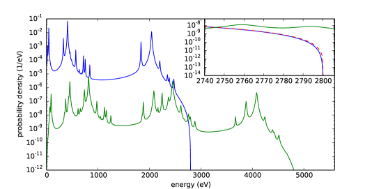
Figure 1: De-excitation spectrum from ¹⁶³Ho electron capture, based on one- and two-hole states [4], energy endpoint $Q=2800$ eV, and neutrino mass $m(\nu_{\text{e}})=0$ eV, is shown (blue) along with its self convolution (green), the spectrum of a piled-up pair. Latter is scaled by the relative probability $3.00\times 10^{-4}$ of pile-up from an event rate of 300 /s and time resolution of 1 $\mu$s. Inset focuses on energies of interest near $Q$ and adds single-event spectrum for $Q=2801$, $m(\nu_{\text{e}})=1$ eV (red, dashed). In an experiment, just the sum of single-pulse and pile-up spectra is observable. (Color figure online.)

1 Introduction

Experiments attempting direct measurement of the electron anti-neutrino mass $m(\nu_{\text{e}})$, including ECHo [1], HOLMES [2], and NuMECS [3], which measure the de-excitation energy of ¹⁶³Dy produced by ¹⁶³Ho electron capture, seek to quantify the spectrum of this de-excitation energy, after neutrino escape, near its endpoint $Q-m(\nu_{\text{e}})$ where its shape is sensitive to $m(\nu_{\text{e}})$. HOLMES experiment specifications, for example, are for 300 events per detector per second with time resolution of 1 $\mu$s to separate distinct events, but under these conditions misleading piled-up events with energy sum in the vicinity of $Q-m(\nu_{\text{e}})$ are more prevalent than single events with similar energy; see Fig. 1. Minimizing erroneous counting of double events as single is crucial to the success of these experiments.

A TES microcalorimeter, heated by the energy of an arriving particle, traverses a sharp transition in resistance from its bias point near superconductivity toward normal resistance; this change is observed as a drop in current through the device, with pulse onset and decay rates determined largely by circuit inductance and thermal conductance to a heat bath. A rapid pulse rise, facilitating pile-up detection, is one strategy to reduce undetected pile-up of pulses, but at a given sample rate there is a trade-off between pulse rise time and effective energy resolution. Another strategy is optimal (Wiener) filtering [5] to invert the effect of detector linear impulse response and additive colored Gaussian noise. Obstacles in practice, however, of detector nonlinear response, pulse rising-edge readout distortion tied to event sub-sample arrival time [6], and inherent instability of Wiener filter construction due to uncertainty of pulse shape and noise power spectrum, motivate exploration of alternative methods.

Simulations demonstrate the efficacy of a new approach based on singular value decomposition (SVD), both to distinguish piled-up pulse records from more numerous single-pulse records in training data and to construct a model of the single-pulse records for use in identifying relatively much more numerous piled-up records near the energy-spectrum endpoint. For sample spacing $\Delta t$ we observe time resolution near $\Delta t/2,$ which we argue below is ideal. By comparison, the time resolution of Wiener filtering is observed [7] as approximately $\Delta t$.

2 Energy Spectrum, Detector Model, and Processing Procedure

2.1 Energy spectrum

Electron capture by ¹⁶³Ho yields excited ¹⁶³Dy whose de-excitation energy spectrum (Fig. 1) has probability density

$$\frac{\text{d}\Gamma}{\text{d}E}=(Q-E)\sqrt{(Q-E)^{2}-{m(\nu_{\text{e}})}^{2}}\sum_{f}\frac{\lambda_{0}B_{f}\Gamma_{f}}{2\pi\left[(E-E_{f})^{2}+{\Gamma_{f}}^{2}/4\right]}$$ (1)

well established theoretically [8]. Total energy $Q$ and triples $E_{f},B_{f},\Gamma_{f},$ specifying center, amplitude, and width of the Lorentzians comprising terms of the summation, have been determined experimentally and computationally, with recent major improvements in determining line locations and widths [9], second- and third-order transitions [4,10,11,12], and $Q$ [13].

In the following we omit third-order electron transitions from simulation.

2.2 Detector model

For this study we simulate current pulses in a transition-edge-sensor (TES) microcalorimeter. The dynamics of detector temperature $T$ and current $I$ are modeled by ordinary differential equations

$$C\frac{\text{d}T}{\text{d}t} =-k\cdot(T^{n}-{T_{\text{bath}}}^{n})+I^{2}R(T,I)+\sum_{i}\delta\left(t-t_{i}\right)\cdot E_{i}$$ (2)

$$L\frac{\text{d}I}{\text{d}t} =V-I\cdot R_{\text{L}}-I\cdot R(T,I)$$ (3)

of the Irwin-Hilton model [14], for energies $E_{1},E_{2},\ldots,$ arriving at times $t_{1},t_{2},\ldots,$ with detector resistance given by the formula

$$R(T,I)=\frac{R_{\text{N}}}{2}\left[1+\text{tanh}\left(\frac{T-T_{\text{c}}+(I/A)^{2/3}}{2\text{ln}(2)T_{\text{w}}}\right)\right]$$ (4)

proposed by Shank et al. [15], with the small-signal linearizations [14] of the transition—logarithmic temperature sensitivity $\alpha$ and logarithmic current sensitivity $\beta$ of detector resistance $R$ at quiescence—replaced by the functional form of Eq. (4). Physical parameters in Eqs. (2)–(4) are chosen to be similar to those of detectors being developed [16] at NIST for HOLMES, specifically

Assumed:
$n=3.25$	$T_{\text{c}}=0.1$ K	$T_{\text{bath}}=0.07$ K
$k=23.3$ nW/Kn	$C=0.5$ pJ/K	$L\in\{12,24,48\}$ nH
$R_{0}=2$ m$\Omega$	$R_{\text{L}}=0.3$ m$\Omega$	$R_{\text{N}}=10$ m$\Omega$
$\alpha=\partial\ln R/\partial\ln T\big{|}_{0}=200.0$	$\beta=\partial\ln R/\partial\ln I\big{|}_{0}=2.0$
Derived:
$T_{0}=0.0980$ K	$I_{0}=63.85\;\mu$A	$G=406.8$ pW/K
$T_{\text{w}}=0.565$ mK	$A=1.133$ A/K3/2	$V=146.9$ nV.

Temperature at quiescence $T_{0}$ is obtained from $\alpha,$ $\beta,$ $R_{0},$ and Eq. (4). Current at quiescence $I_{0}$ is then obtained from temperature balance and parameters $T_{\text{w}}$ and $A$ are obtained from $T_{0},$ $I_{0},$ $R_{0},$ $\alpha,$ and $\beta$, while $G=\partial\left[k\cdot(T^{n}-{T_{\text{bath}}}^{n})\right]/\partial T\big{|}_{0}$ $=kn{T_{0}}^{n-1}.$

Three values of inductance, $L=12,\;24,\;48$ nH, are simulated to enable evaluation of pile-up detection contrasting relatively rapid with relatively slow pulse rises, the latter allowing lower sample rates. Pulse shape and detector nonlinearity are shown in Fig. 2.

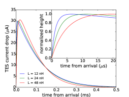
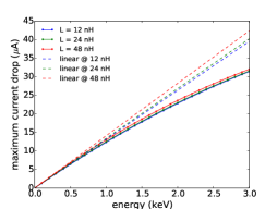
Figure 2: Pulse shape at 2.8 keV, with rising-edge detail (Left) and linearity of pulse height versus energy with slope from 0.1 keV (Right) for inductances 12, 24, 48 nH. The proposed pile-up detection approach achieves near-ideal performance on all three. (Color figure online.)

Noise is additive with power spectrum given by the Irwin-Hilton model [14], which depends on TES circuit inductance, and is generated in the simulation as an autoregressive moving average (ARMA) process on Gaussian white noise. The noise spectra are shown in Fig. 3.

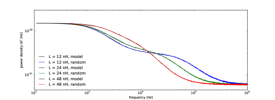
Figure 3: Noise power spectrum—from Irwin-Hilton model and from simulation by ARMA process—for inductances $L=12,\;24,\;48$ nH. (Color figure online.)

2.3 Generation of events and pile-up

We simulate events according to the one- and two-hole electron excitation spectrum [4] with endpoint $Q=2.8$ keV (motivated by the recent independent measurement of $Q$ [13]), neutrino mass $m(\nu_{\text{e}})=0$ eV, and event mean arrival rate $\lambda=300$ /s. Detecting pile-up is of particular importance for identifying the single pulses for energies near $Q,$ which carry the information on $m(\nu_{\text{e}})$. To obtain a sufficient number of counts, we restrict generation of each single-pulse energy $E$ to the interval $S_{\text{E}}=[2.70,2.82]$ keV. Piled-up pairs, with lag $t_{\Delta}$ between arrival times of less than $\delta=10$ $\mu$s and each event drawn from the full energy spectrum, subject to the sum of their energies $E_{1}+E_{2}$ lying in $S_{\text{E}},$ have rate fraction

$$f_{\text{pp}}=\frac{c_{\text{pp}}}{c_{\text{s}}+c_{\text{pp}}}$$ (5)

where $c_{\text{s}}$ is the count of single and $c_{\text{pp}}$ the count of piled-up pulse pairs. These incidence frequencies are determined by the probabilities

$$\text{Pr}(E\in S_{\text{E}})=6.78\times 10^{-7},\;\;\text{Pr}(t_{\Delta}\geq\delta)=0.997,$$

$$\text{Pr}(E_{1}+E_{2}\in S_{\text{E}})=2.14\times 10^{-3},\;\;\text{Pr}(t_{\Delta}<\delta)=3.00\times 10^{-3},$$

arising from the ¹⁶³Ho energy spectrum of Eq. (1) and the exponential distribution $F(t)=1-\lambda\text{e}^{-\lambda t}$ of time lags for Poisson arrivals. Therefore

$$f_{\text{pp}}=\frac{\text{Pr}(E_{1}+E_{2}\in S_{\text{E}})\text{Pr}(t_{\Delta}<\delta)}{\text{Pr}(E_{1}+E_{2}\in S_{\text{E}})\text{Pr}(t_{\Delta}<\delta)+\text{Pr}(E\in S_{\text{E}})\text{Pr}(t_{\Delta}\geq\delta)}=0.905$$ (6)

and only after detection and rejection are pile-ups less numerous than single-pulse records.

Once arrival times and event energies are generated, a stream of samples of current $I$ is obtained by solution of ordinary differential equations of Eqs. (2), (3) by explicit fourth-order Runge-Kutta integration on nodes with uniform spacing $\Delta t=0.5\;\mu$s in addition to nodes at event arrival times—where model temperature $T$ is discontinuous—and the uniform nodes are retained. These samples are subsequently decimated to obtain sample rates of 2, 1, 0.67, and 0.5 MHz.

2.4 Recordization

After ARMA-generated noise is added to the samples, the stream of samples is formed into pulse records, simulating conditions of the physical experiment. Pulse arrivals are determined by a six-sample pulse trigger in which a line segment is fit to the first five samples and a threshold is applied to the difference between the sixth sample and the advanced line height. This procedure enables detection of a pulse arrival just five samples after a prior arrival, including on the rising edge of the prior pulse. A pulse record of duration 0.5 ms is formed, provided that 0.1 ms before and 0.4 ms after a pulse arrival are free of other triggered arrivals. Records that have relatively flat pre-trigger are retained and transformed to whiten noise by a fast Cholesky-factor backsolve procedure [17].

2.5 Pile-Up detection

Our strategy for pile-up detection is to develop a model of single-pulse records and reject as piled-up those records whose model fit has too-large residual. The energy interval $S_{\text{E}}$ has ¹⁶³Ho single-pulse record counts dominated by piled-up-record counts, as is evident from Eq. (6); our models built from single-pulse-dominated intervals at lower energies (for example, near the 2.042 keV spectral peak) were not effective on $S_{\text{E}}$. Instead we propose adding a switchable source of photons [18], from L$\alpha$ x-ray emission lines of Ru (2.683, 2.688 keV) and Pd (2.833, 2.839 keV), likely also of value as reference lines for combining data of multiple detectors. A second simulation, for the energy interval $S^{\prime}_{\text{E}}=[2.65,2.87]$ keV, with the switchable source in combination with ¹⁶³Ho to provide approximately five times as many separated pulses as piled-up pairs, is used as a training set for developing a single-pulse model (see Fig. 4).

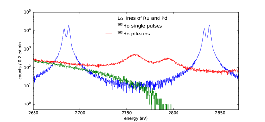
Figure 4: De-excitation spectra from ¹⁶³Ho electron capture have single pulse counts (green) heavily dominated by pile-up counts (red) near $Q$ in expected physical data and in simulation according to Eq. (6) (shown). (Unlike Fig. 1, which assumes 1 $\mu$s time resolution, the training data are shown prior to pile-up detection.) Therefore to enable construction of a single-pulse model, in a model training phase the ¹⁶³Ho source is augmented with a source yielding single pulse counts (blue) from L$\alpha$ x-rays of Ru and Pd. (Color figure online.)

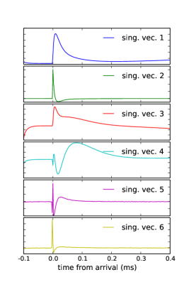
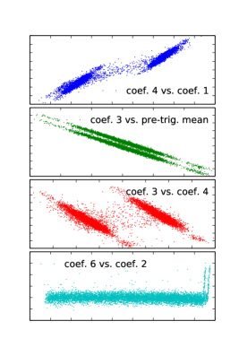
Figure 5: Left: Singular vectors linked to largest singular values enable representation of variations due to pulse amplitude, sub-sample arrival time, and baseline shifts, with nonlinear effects, while suppressing noise. Right: Certain of their coefficients correlate, providing redundancy to allow evaluation of pulse record conformance to a single-pulse model. (Color figure online.)

2.5.1 Separating single-pulse records

The model training simulation yields records that, while containing more single pulses than pile-ups, are not governed by single pulses adequately to enable direct construction of a single-pulse model. We therefore precede model construction with a step in which piled-up records are identified as outliers and removed.

The singular value decomposition (SVD) $M=UDV^{t}$ is computed for a matrix $M$ whose columns consist of pulse records (Fig. 5). The first $j$ columns ($j<10$) of $U$ comprise a good basis for the full set of records; the remaining columns are dominated by noise, as signaled by the very slow decay of the singular values beyond the $j$th. The means of the first $j$ columns of $V$ are subtracted from those columns to obtain $\hat{V}.$ The $j\times j$ empirical covariance $\hat{\sigma}^{2}=\hat{V}^{t}\hat{V}$ is then used to obtain a squared deviation $d^{2}=\hat{V}_{i,*}(\hat{\sigma}^{2})^{-1}\hat{V}_{i,*}^{t}$ of each record $i$. Piled-up records deviate disproportionately from the mean in this covariance-adjusted sense so we discard those with largest $d^{2},$ and repeat the procedure on the remaining records (form $M,$ compute SVD $M=UDV^{t}$ and each $d^{2}$, discard records with largest $d^{2}$) a total of three times, with $m/2$ discards on the first iteration, $m/4$ on the second, and $m/8$ on the third, where $m$ is the expected number of piled-up records. The value of $m$ can be estimated as the pile-up count in the stream data (as in Eq. (6) of §2.3) minus the number of removals by the recordization process.

The iterations yield bases computed by SVD that successively improve the representation of single-pulse records, as piled-up records are increasingly eliminated. The three iterations and the sequence of record counts removed per iteration were chosen empirically to generate a balance between false positives—single-pulse records discarded as piled up—and false negatives—piled-up records retained as single pulses.

Table 1: Initial (pp${}_{\text{i}}$) and final (pp${}_{\text{f}}$) pile-up record count fractions of training and evaluation data sets, energy resolution $\Delta E$ (FWHM), and effective time resolution $\tau_{\text{R}}$. Columns labelled F$+$ and F$-$ are the false positives—single-pulse records discarded as piled up—and false negatives—piled-up records retained as single pulses. Energy is computed by optimal filtering [19] and $\tau_{\text{R}}$ is the ratio of number of retained piled-up records to single-pulse records, divided by that ratio of original events ($1\,083\,229$ / $114\,049$), times $\delta=10\;\mu$s.

MHz	count fractions (training)				$\Delta E$	count fractions (evaluation)				$\tau_{\text{R}}$
nH	pp${}_{\text{i}}$	F$+$	F$-$	pp${}_{\text{f}}$	(eV)	pp${}_{\text{i}}$	F$+$	F$-$	pp${}_{\text{f}}$	($\mu$s)
2.0
12	.042	.002	.172	.007	1.99	.681	.009	.139	.231	0.29
24	.048	.002	.167	.008	2.10	.707	.013	.225	.355	0.31
48	.054	.002	.162	.009	2.31	.724	.011	.243	.391	0.49
1.0
12	.073	.002	.153	.012	2.46	.796	.010	.140	.355	0.55
24	.081	.002	.151	.013	2.45	.813	.010	.131	.366	0.56
48	.087	.005	.173	.016	2.60	.824	.011	.136	.391	0.60
0.67
12	.101	.005	.174	.019	3.34	.849	.008	.145	.451	0.83
24	.109	.003	.153	.018	2.76	.859	.009	.133	.450	0.81
48	.112	.005	.168	.021	2.80	.864	.007	.142	.476	0.84
0.5
12	.127	.009	.185	.027	7.54	.880	.006	.150	.525	1.11
24	.130	.007	.175	.026	3.17	.883	.007	.142	.518	1.09
48	.124	.009	.189	.026	2.89	.877	.006	.160	.534	1.08

2.5.2 Constructing single-pulse model

The separation procedure culls the collection of training records so that nearly all of those remaining are single-pulse records, which enables construction of a single-pulse model. The SVD $M=UDV^{t}$ is again computed and the first $j$ of the expansion coefficients $(VD)_{i,*}$ for record $i$ are augmented with the record’s pre-trigger mean. The first column of $U$ approximates the average pulse, while the second column is dominated by the effect of varying arrival time on pulse shape. The remaining basis vectors encode variations due to changing baseline and to nonlinear effects of varying pulse height, arrival time, and baseline, so we approximate expansion coefficients $3,\ldots,j$ by linear regression from a nonlinear space from coefficients 1, 2, and the pre-trigger mean. In particular, naming these three independent variables $x,\;y,\;z,$ we construct a model for each of the $j-2$ dependent variables as a linear combination of $1,\;x,\;y,\;z,\;xy,\;yz,\;zx,\;xyz,$ resulting in $8\cdot(j-2)$ model coefficients.

The model residual is obtained for each training record and, more importantly, for any pulse record, when $j$ expansion coefficients (along with pre-trigger mean) are computed by taking the inner product of the record with the basis vectors. Records with residual norm above a threshold are deemed piled-up, where the threshold is chosen to include 99 % of the training set pulse records that survive as single pulsed. A lower threshold would yield only a few more detected pile-ups.

For both training steps, of separating single-pulse records and of constructing the single-pulse record model, we choose $j=6$. Readout distortion on the pulse rising edge [6]—not modeled here—likely will imply $j>6$ in the physical setting.

2.5.3 Energy bias of pile-up detection

After pile-up detection and rejection, many records with pile-up remain—false negatives—and some single-pulse records are discarded—false positives. Correct analysis of the experiment therefore requires assessing the extent of energy bias inherent in the pile-up detection procedure.

Initially attempting graphically to estimate the bias, as a function of energy, of the detection procedure, we find good agreement between the distributions of accepted and rejected records across the energy interval $S_{\text{E}}$.

We then compare the energy distribution of retained single-pulse records to that of all other generated single pulses, and the distribution of retained piled-up records—with the two energies summed—to that of all other generated pile-ups, by means of the two-sample Kolmogorov-Smirnov distribution-equality test.

3 Simulation Results

Table 1 shows initial and final pile-up record count fractions, and false positive and false negative count fractions, for training and evaluation data. In addition, the energy resolution $\Delta E$ and effective time resolution $\tau_{\text{R}}$ of the procedure are shown. We note that pulses of the 12 nH inductance models—with fastest rise—are poorly resolved at the lower sampling rates. This leads to poor energy resolution $\Delta E$, but the time resolution $\tau_{\text{R}}$ after pile-up detection suffers only slightly. Also, not shown here, varying the noise level affects $\Delta E$ significantly, but $\tau_{\text{R}}$ just slightly.

Fig. 6 shows the undetected piled-up record counts as a function of event arrival lag $t_{\Delta}$ for the 12 cases. These plots make clear that, regardless of pulse shape variation and noise, the performance of the pile-up detection depends closely on whether or not there is at least one sample between two event arrivals. Achieved time resolution $\tau_{\text{R}}$ shown in Table 1 can be compared with values of 0.25, 0.50, 0.75, and 1.00 $\mu$s—half the sample spacing—for sampling rates of 2.0, 1.0, 0.67, and 0.5 MHz, respectively. This criterion characterizes ideal performance, since under the temperature-current model of Eqs. (2)–(3), two arrivals with no intervening sample cannot be distinguished from a single arrival with energy roughly the sum of the two energies.

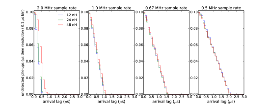
Figure 6: Undetected piled-up record counts are shown as a function of time lag $t_{\Delta}$ between arrivals of the first and second events of a pair. (Vertical scale results from 0.1 $\mu$s arrival-lag bin size.) One sample between arrivals generally enables their detection as a pair, resulting in the nearly linear dependence seen. (Color figure online.)

The Kolmogorov-Smirnov test (at 95 % level) of energy bias in retaining single-pulse records failed to reject the null hypothesis—equivalent to no bias—for all 12 data sets. The test for energy bias in retaining piled-up records failed to reject the null hypothesis for 7 of the 12 data sets, which suggests energy bias on 5 of the 12. The bias, like the energy resolution and unlike the time resolution, is sensitive to the noise level, with lower noise producing less bias. Preferable to a hypothesis test would be determination of the effect of bias on the final estimate of the quantity of interest $m(\nu_{\text{e}})$, which is important for other pile-up detection methods as well. We undertake this analysis and present its results elsewhere.

4 Conclusions

These simulations show that there is approximately a two-fold reduction in pile-up, after rejection, compared with Wiener filtering. The improvements provided by these algorithms, based on SVD, have significant, beneficial implications for planned and future experiments that employ calorimetric sensors to measure the neutrino mass. For current experiments with a defined number of pixels such as HOLMES, this improved pile-up rejection enables a lower sampling rate per detector, thus relaxing the requirements on the multiplexing readout system and subsequent detector speeds, while providing similar or improved reduction in uncertainty due to pile-up and therefore better constraint on the neutrino mass. In future experiments, where the measurement uncertainty due to pile-up will be better understood, a lower sample rate will allow more detectors to be multiplexed per readout channel for the specified time resolution requirement. This capability reduces the total number of necessary multiplexing channels and will allow for larger arrays of detectors in a single cryogenic cooler, thus reducing both the cost and complexity and enhancing the feasibility of such experiments.

Acknowledgements The NIST Innovations in Measurement Science program and the European Research Council, funding HOLMES, supported this work. The authors also thank Kevin Coakley, Galen O’Neil, and Hideyuki Tatsuno for helpful comments on a draft of this paper.

References

- 1 L. Gastaldo et al., J. Low Temp. Phys. 176 876 (2014), doi:10.1007/ s10909-014-1187-4.
- 2 B. Alpert et al., Eur. Phys. J. C 75 112 (2015), doi:10.1140/epjc/s10052-015-3329-5.
- 3 G. Kunde et al., J. Low Temp. Phys. This Special Issue (2015).
- 4 A. Faessler and F. S̆imkovic, Phys. Rev. C 91 045505 (2015), doi:10.1103/PhysRevC.91. 045505.
- 5 See, for example, M. Vetterli and J. Kovacevic, Foundations of Signal Processing, Cambridge University Press (2014)
- 6 J. W. Fowler et al., J. Low Temp. Phys. This Special Issue (2015)
- 7 E. Ferri et al., J. Low Temp. Phys. This Special Issue (2015)
- 8 A. DeRujula and M. Lusignoli, Phys. Lett. B 118 429 (1982), doi:10.1016/0370-2693(82) 90218-0.
- 9 P.C.-O. Ranitzsch et al. J. Low Temp. Phys. 167, 1004 (2012) doi:10.1007/s10909-012-0556-0.
- 10 R. Robertson, Phys. Rev. C 91 035504 (2015), doi:10.1103/PhysRevC.91.035504.
- 11 A. Faessler, L. Gastaldo, and F. S̆imkovic, IOP J. Phys. G 42 015108 (2015), doi:10.1088/0954-3899/ 42/1/015108.
- 12 A. Faessler et al., Phys. Rev. C 91 064302 (2015), doi:10.1103/PhysRevC. 91.064302.
- 13 S. Eliseev et al., Phys. Rev. Lett. 115, 062501 (2015) doi:10.1103/PhysRevLett.115.062501.
- 14 K. Irwin and G. Hilton in Cryogenic Particle Detection, C. Enss (Ed), Springer-Verlag (2005)
- 15 B. Shank et al., AIP Advances 4 117106 (2014), doi:10.1063/1.4901291.
- 16 J. Hays-Wehle et al., J. Low Temp. Phys. This Special Issue (2015)
- 17 J. Fowler et al., Astrophysical Journal Supplement Series 219 35 (2015), doi: 10.1088/0067-0049/219/2/35.
- 18 C. de Vries et al., Proc. SPIE 8443 844353 (2012), doi:10.1117/12.924146.
- 19 A. E. Szymkowiak et al., J. Low Temp. Phys. 93, 281–285 (1993), doi:10.1007/ BF00693433.