SP_Ace: a new code to derive stellar parameters and elemental abundances
Abstract
Context. Ongoing and future massive spectroscopic surveys will collect large numbers (-) of stellar spectra that need to be analyzed. Highly automated software is needed to derive stellar parameters and chemical abundances from these spectra.
Aims. We developed a new method of estimating the stellar parameters , , [M/H], and elemental abundances. This method was implemented in a new code, SP_Ace (Stellar Parameters And Chemical abundances Estimator). This is a highly automated code suitable for analyzing the spectra of large spectroscopic surveys with low or medium spectral resolution (R=2 000-20 000).
Methods. After the astrophysical calibration of the oscillator strengths of 4643 absorption lines covering the wavelength ranges 5212-6860Å and 8400-8924Å, we constructed a library that contains the equivalent widths (EW) of these lines for a grid of stellar parameters. The EWs of each line are fit by a polynomial function that describes the EW of the line as a function of the stellar parameters. The coefficients of these polynomial functions are stored in a library called the “ library”. SP_Ace, a code written in FORTRAN95, uses the library to compute the EWs of the lines, constructs models of spectra as a function of the stellar parameters and abundances, and searches for the model that minimizes the deviation when compared to the observed spectrum. The code has been tested on synthetic and real spectra for a wide range of signal-to-noise and spectral resolutions.
Results. SP_Ace derives stellar parameters such as , , [M/H], and chemical abundances of up to ten elements for low to medium resolution spectra of FGK-type stars with precision comparable to the one usually obtained with spectra of higher resolution. Systematic errors in stellar parameters and chemical abundances are presented and identified with tests on synthetic and real spectra. Stochastic errors are automatically estimated by the code for all the parameters. A simple Web front end of SP_Ace can be found at http://dc.g-vo.org/SP_ACE, while the source code will be published soon.
Key Words.:
Methods: data analysis – Atomic data – Stars: fundamental parameters – Stars: abundances – Techniques: spectroscopic – surveys1 Introduction
The physical, chemical, and kinematic information carried by the stellar spectra are fundamental for understanding how the Milky Way formed and evolved. The increasing demand for stellar spectra by astronomers engaged in Galactic archaeology led to large spectroscopic surveys that could be carried out thanks to the availability of efficient multi-object spectrographs, to the fast growth of the data storage capability, and the computational power of modern computers. Past, present, and future surveys (such as the RAdial Velocity Experiment, RAVE, rave, 2006, Steinmetz at al.; the Sloan Extension for Galactic Understanding and Exploration, SEGUE, yanny, 2009, Yanny et al.,; the Large Sky Area Multi-Object Fiber Spectroscopic Telescope, LAMOST, zhao, 2012, Zhao et al.; The Apache Point Observatory Galactic Evolution Experiment, APOGEE, apogee, 2008, Allende Prieto et al.; the Galactic Archaeology with HERMES-GALAH Survey, zucker, 2012, Zucker et al.; the Gaia-ESO Public Spectroscopic Survey, gilmore, 2012, Gilmore et al.; the 4-Metre multi-Object Spectroscopic Telescope, 4MOST, dejong, 2012, de Jong et al.; Gaia, perryman, 2001, Perryman et al., lindegren, 2008, Lindegren et al.) delivered and will deliver millions of stellar spectra that need to be analyzed to derive stellar parameters (effective temperatures , gravity , metallicity [M/H]) and elemental abundances. The analysis of such an amount of data is a challenge that can be addressed by its automation. Today there is considerable effort to develop software for this purpose.
Some software packages implement the classical spectral analysis by measuring equivalent
widths (EW) of isolated, well known absorption lines and by deriving
stellar parameters from the excitation equilibrium and ionization balance
(such as the Fast Automatic Moog Analysis, FAMA, magrini, 2013, Magrini et
al.; GALA, mucciarelli, 2013, Mucciarelli et al.;
ARES sousa, 2007, Sousa et al.).
These programs are particularly oriented to
high-resolution, high signal-to-noise (S/N) spectra, for which isolated lines
can be recognized, and their EW can be reliably measured thanks to a safe
continuum placement.
Other methods are based on grids of synthetic spectra, but they
differ in the “line-fitting” or “full-spectrum-fitting” approach, i.e.,
by fitting isolated absorption lines one-by-one (e.g., MyGIsFOS,
sbordone, 2014, Sbordone et al.; Stellar Parameters
Determination Software, SPADES, posbic, 2012, Posbic et al.), or
by fitting full spectral ranges (e.g., the MATrix Inversion for Spectral SynthEsis, MATISSE,
recio-blanco, 2006, Recio-Blanco et al.; neural networks, among others
statnet by bailer-jones, 1996, Bailer-Jones;
FERRE, allendeprieto, 2006, Allende Prieto et al.).
Spectroscopy Made Easy (SME, valenti, 1996, Valenti & Piskunov)
distinguishes itself from the other codes since it
synthesizes on-the-fly single absorption lines or parts of the
spectrum to be matched with the observed ones.
The line-fitting analysis can derive stellar
parameters and chemical abundances with the drawback of neglecting the
significant amount of information carried by the unused part of the
observed spectrum. This penalizes the line-fitting approach to low S/N, low
metallicity, and low resolution spectra, in which the number of usable lines
may be too small to carry out this analysis.
On the other hand, the full-spectrum-fitting approach cannot deliver
chemical abundances
because the grid of synthetic spectra needed to cover the
whole parameter and chemical space (and account for
many elemental abundances) would be too big to be handled
111The ASPCAP pipeline can derive
abundances for up to 15 elements with a technique that can be classified as
a line-fitting approach. See Elia Garcia Perez et al.
eliagarciaperez (2014)..
Other techniques can use real spectra as templates
(“The Cannon”, ness, 2015, Ness et al.; ULySS, koleva, 2009, Koleva et
al.) with the advantage of overcoming the systematic errors that
stem from the synthetic spectra (due to our incomplete knowledge of atomic parameters
and stellar atmospheres) but share with the previous techniques the
challenge to collect a number of templates
large enough to uniformly cover the stellar parameter and chemical space.
The accuracy of the parameters derived with any of the methods proposed so far (including this work) depends on two fundamental pillars: the precision and accuracy of i) the atomic parameters of the absorption lines employed and ii) the reliability of the stellar atmosphere models. In both these areas, significant progress has been made in recent years, and because of their importance, they deserve further support. The recent praiseworthy efforts to supply laboratory oscillator strengths (ruffoni_ges, 2014, Ruffoni et al., but see also other works cited later on) cover a number of lines that may meet the needs of the classical spectral analysis (i.e., the line-fitting approach), but these are too few for the needs of a full-spectrum-fitting analysis. On the other hand, the 3D stellar atmosphere modeling (asplund2005, 2005, Asplund; freytag, 2012, Freytag et al.; magic, 2013, Magic et al.) show that realistic model atmospheres can reproduce the observed spectra with great accuracy. However, the computational power required today to analyze wide spectral ranges with these tools is prohibitive.
To this lively field that is rich in new ideas, we contribute with a software called SP_Ace (Stellar Parameters And Chemical abundances Estimator) that implements a new method of performing stellar spectral analysis. SP_Ace is based on a method born from the experience of the RAVE chemical pipeline (Boeche et al. boeche11, 2011) developed to derive elemental abundances from the spectra of the RAVE survey (Steinmetz et al. rave, 2006; Kordopatis et al. kordopatisDR4, 2013). The RAVE chemical pipeline relies on stellar parameters that must be provided by other sources, and it only derives chemical abundances. SP_Ace extends the RAVE chemical pipeline’s foundations and performs an independent, complete spectral analysis. Although SP_Ace employs a full-spectrum-fitting approach, it derives stellar parameters as much as chemical elemental abundances for FGK-type stars. Unlike other codes dedicated to stellar parameter estimation, SP_Ace does not rely on a library of synthetic spectra, or measure the EW of absorption lines, but it makes use of functions that describe how the EW of the lines changes in the parameter and chemical space. In the next section we explain the general concepts on which SP_Ace is based.
2 Method
The usual methods employed to estimate stellar parameters from spectra are i)
to directly compare the observed spectrum with the synthetic one to find
the best match and ii) to measure the EWs of the absorption lines of the
observed spectrum from which the stellar parameters are inferred.
In both cases the spectrum must be synthesized, and the stellar parameters of the
synthetic spectrum are varied until the spectrum (first case) or
the line’s EWs (second case) match the observed ones. Any spectrum synthesis
depends on a stellar atmosphere model,
that represents the physical conditions in the stellar atmosphere to
the best of our knowledge.
For this reason stellar parameters and chemical abundances obtained from spectral
analysis are indirect measurements, and we say that they are derived (and not
measured).
Regardless of the method employed, to estimate the stellar parameters from spectra
we must construct a spectrum model and compare it to the observed
spectrum. SP_Ace makes no exception: it constructs a spectrum model
and compares it with the observed spectrum with a simple analysis.
Its peculiarity is the novel way to construct the spectrum model, which is
not a direct synthesis. At first glance this method may look cumbersome, but it
eventually gives consistent advantages that we describe below.
Consider a stellar spectrum of low to medium spectral resolution222In the following the spectral resolution at wavelength is defined as R, where is the Full-Width-Half-Maximum (FWHM) of the instrumental profile. () with a known instrumental profile. An absorption line can be fit with a Voigt profile of known FWHM and strength (i.e., EW). We start from the naïve idea that a normalized spectrum can be reproduced by subtracting Voigt profiles of appropriate wavelengths, FWHMs, and EWs from a constant function equal to one (representing the normalized continuum). Under the weak line approximation the spectrum so constructed would reproduce the observed spectrum with fair precision333We here want just outline the main idea. To generalize the method the weak line approximation must be removed, and this is discussed in Sec. 5.. To construct a full spectrum in this way we need to know the EWs of the lines at the wanted , , and abundance [El/H]444We define chemical abundance of a generic element “El” as [El/H]= where is the number of particle per unit volume. of the generic element “El” the lines belong to. For this purpose we synthesize the lines for a grid of stellar parameters , , and chemical abundance [El/H]555The microturbulence employed is a function of and as clarified in Appendix A., measure the EWs at such points, and store them into a library that we called the EW library. The EW library contains all the information that describes the strength of the lines in the stellar parameter and chemical space. So defined, the EW of an absorption line is a function of the stellar parameters that we call General Curve-Of-Growth (GCOG) to remember that it is the generalization of the well known Curve-Of-Growth (COG) function (which can be obtained from the GCOG by fixing the parameters and , and leave the abundance [El/H] as free variable). By using the EW library we can construct spectrum models with stellar parameters and abundances corresponding to grid points of the library. To overcome the discreteness of the grid in the parameter space, we use continuous functions that fit the EWs of the lines in the parameter and chemical space. This can be done with polynomial functions that we call “polynomial GCOGs” and that we store in the “GCOG library”. The advantage of this method is that we just need to vary the parameters , , and abundances [El/H] in the polynomial GCOGs to vary the strength of the lines and construct spectrum models for any stellar parameters and abundances until we find the one that matches the observed spectrum best666The difference to the RAVE chemical pipeline (Boeche et al. boeche11, 2011) is that this one takes and as external input and uses polynomial COGs to only derive chemical abundances.. This method is implemented in the code that we call SP_Ace.
To achieve this result, three steps are necessary: i) to build a line list of
absorption lines that must be as much complete as possible (possibly all the
lines visible in stellar spectra) ii) to build an EW library where the EWs of
every absorption line are stored as a function of , , and [El/H], and
iii) to use the EW library to fit the polynomial GCOGs and store their
coefficients in the GCOG library that is employed by the code SP_Ace to construct the
spectrum model. These steps are outlined in the next sections.
3 The line list
To build the EW library we need a list of atomic and molecular absorption lines and their physical parameters. These physical parameters are: wavelength, atom or molecule identification, oscillator strength (, often expressed as logarithm , where is the statistical weight), excitation potential (), van der Waals damping constant , and dissociation energy (only for molecules). The atomic line list was taken from the Vienna Atomic Line Database (VALD, Kupka et al. kupka, 1999), with the option that selects the lines with expected strengths larger than 1% in at least one of the normalized spectra of the Sun, Arcturus, and Procyon777The VALD web interface lists the lines which strengths are larger than 1% of the normalized flux of a synthetic spectrum which stellar parameters correspond to the nearest point of the stellar parameters grid to the stellar parameters provided by the user. For instance, for the Sun the closest grid point is at =5750 K, =4.5, [M/H]=0 dex.. Afterwards, the EWs of these lines were re-computed with the code MOOG (Sneden sneden, 1973) and only the lines with EW1mÅ in at least one of these stars were included in the line list. The molecular line list was taken from Kurucz kurucz (1995) and selected with the same procedure employed for the atomic lines. In the present work the line list covers the wavelength intervals 5212-6860Å and 8400-8924Å. We chose the first interval because it is commonly covered by optical spectra, while the second interval (the Ca II triplet region) becomes particularly important because of Gaia spectral coverage. Extentions of the line list to other wavelength ranges can be done in the future.
3.1 The atomic lines
The wavelengths and excitation potentials were adopted from the VALD database.
The oscillator strengths are discussed in Sec.4.
The van der Waals damping constants were taken from the VALD database
when such values are available.
When VALD does not provide the damping constants,
we adopted the Unsöld approximation (computed by MOOG) multiplied by
the enhancement factor Eγ following the recipe of Edvardsson et
al. edvardsson (1993) and Chen et al. chen (2000). For the neutral iron
lines Fe I, this recipe assigns E for lines with
eV and E for eV (Simmons & Blackwell
blackwell, 1982), whereas for the ionized Fe II lines E
(Holweger et al. holweger90, 1990). For K I, Ti I, and V I E (Chen et al. chen, 2000), for Na I E
(Holweger et al. holweger71, 1971), for Ca I E (Oneill
& Smith oneill, 1980), for Ba II E (Holweger &
Mueller holweger74, 1974). For any other element,
E (Maeckle et al. maeckle, 1975).
Precise damping constants were computed by Barklem et
al. barklem00 (2000) and Barklem & Aspelund-Johansson barklem05 (2005).
Such values are contained in the MOOG data files and, by setting
the MOOG keyword “damping=1” we imposed to use the Barklem values
when they are available.
There are few cases for which there are no Barklem damping
constants and for which the enhancement factor Eγ does not apply.
These are:
-
•
The strong and broad lines of H I. Our synthesis with MOOG under Local Thermodynamic Equilibrium (LTE) assumptions and one dimensional (1D) stellar atmosphere models (see Sec.4.1 for details) renders a too weak H line at the line core, whereas the synthetic Paschen H I lines in the near infrared are too strong at the tip of the line, and too weak in the wings with respect to the observed lines. For all these lines we adopted the Unsöld approximation and calibrate the s by hand to improve the fit. However, the match between synthetic and observed H I lines remains unsatisfactory and the lines at 6562.797Å, 8467.258Å, 8502.487Å, 8598.396Å, 8665.022Å, 8750.476Å, and 8862.787Å are neglected during the SP_Ace estimation process. The other Paschen H I lines in the interval 8400-8924Å are so weak in our standard stars that they can be neglected in the and range considered.
-
•
For Si I the damping constants reported in VALD appear always too small. In fact, the Si I lines observed in real spectra are always broader than the lines synthesized with the VALD damping constant. Also the value E suggested by Holweger holweger73 (1973) appears too small888This is in contrast with Wedemeyer wedemeyer (2001) who found that the Unsöld approximation can well describe the wings of silicon lines on the Sun.. After some tests, we adopted E which improves the match of the wings in many (but not all) Si I lines.
-
•
For the Mg I lines 8712.682Å, 8717.815Å, and 8736.016Å we adopted E in order to match better their broad wings. These lines are multiplets treated as one line (as explained in the following).
The need for the adjustments of the Eγ just reported was
recognized during the firsts attempts to calibrate the and
applied before the final calibration procedure (
described later in Sec. 4.1).
In the line list there are multiplets where the lines are so close that
they are physically blended. Because lines of multiplets have the same ,
these physically blended multiplets can be described (as a first approximation)
as if they were one single line.
For multiplets with lines closer than 0.1Å we
adopted one single line with the same and wavelength, which
is the average of the multiplet’s wavelengths. As we adopt the
multiplet’s largest , which is afterwards calibrated by the calibration routine (described in Sec.4).
3.2 The molecular lines
Molecular lines of several species are present in the
considered wavelength ranges. While in hot stars molecules
have a very low probability to form and their spectral lines have negligible
strengths, in cool stars molecular lines become important.
In the range 5212-6860Å the spectra of cool stars
show many absorption features that belong to the species CN, CH, MgH, and TiO.
However, the very high number of molecular lines
present in the range 5212-6860Å prevents us from performing a reliable
calibration of their s (this is discussed in Sec. 4.7).
Therefore, in this work we only treat the CN molecule in the wavelength region
8400-8924Å where the CN lines are sparse and
most of them can be identified one by one.
Physical parameters such as wavelengths and excitation potential are
taken from Kurucz kurucz (1995).
The CN molecule dissociation energy eV was taken from Reddy et al. reddy (2003).
Oscillator strengths for the CN were taken from Kurucz and afterwards
calibrated by the calibration routine (Sec.4).
Molecular multiplets are treated like the atomic multiplets (see
Sec.3.1).
4 The calibration procedure
After the preparation of the line list outlined in
Sec. 3 we focus on the accuracy of the -values.
Most of the -values were derived from
theoretical and semi-empirical calculations (e.g., Seaton seaton, 1994;
kurucz_gf, 1975, Kurucz & Peytremann)
which are known to have significant errors (Bigot &
Thévenin bigot, 2006). Although substantial efforts have been and are
currently being made to obtain precise -value from laboratory measurements
(from Blackwell et al. blackwell72, 1972, blackwell76, 1976,
blackwell79, 1979, blackwell82, 1982, to the more recent works by Ruffoni et al.
ruffoni, 2013) the number of lines for which laboratory -values are
available is still small with respect to the number of lines visible in a
stellar spectrum. Besides, the lines targeted for laboratory
measurements are the unblended ones, important for the classical
spectral analysis. This leaves the blended lines uncovered by the laboratory
measurements.
To improve the quality of the numerous (but inaccurate) -values provided by
the theoretical computations, some authors calibrate the oscillator
strengths by setting the -values to match the strength of the
synthetic line with the corresponding line in the Sun spectrum
(among others Gurtovenko & Kostik gurtovenko81, 1981,gurtovenko82, 1982;
Thévenin thevenin89, 1989;thevenin90, 1990; Borrero
et al. borrero, 2003), in two stars like the Sun and
Arcturus (Kirby et al. kirby, 2008; Boeche et al.
boeche11, 2011) or in three stars like the Sun, Procyon and
Eri (Lobel et al. lobel, 2011). Recently, Martins et al. martins (2014)
used the spectra of three different stars (the Sun, Arcturus, and Vega)
and a statistical technique
(the cross-entropy algorithm) to recover the oscillator strengths and broadening
parameters that minimize the difference between the observed spectra and the
synthetic ones. These works employ the idea that, by using more than one
star we can disentangle lines in blends and recover their individual atomic
parameters999This idea was also employed by boeche11, 2011, Boeche et al.
for the calibration alone, but using a less sophisticated method..
For our line list we decided to calibrate
the oscillator strengths of any blended or isolated line on five different
stellar spectra.
This is necessary because SP_Ace employs a full-spectrum-fitting analysis,
and the few lines with reliable oscillator strengths
available would not be sufficient.
In the following we outline our calibration method. This method
compares the strengths of the synthetic lines with
two (or more) stellar spectra in order to correct the values of isolated
and blended lines. The method was first proposed in
Boeche et al. boeche11 (2011) and we report it here.
In the framework of 1D atmosphere models and LTE assumptions, the EW of a line is a
function of parameters such as , , the abundance [El/H], the excitation
potential , the -value, the damping
constant, and the microturbulence . Given the atomic parameters
and damping constant C6, and assuming that we know with good accuracy the stellar
parameters , , [El/H], and of the stars employed, the EW of a line
can be described as a function of alone
| (1) |
Since we know the stellar parameters of the Sun,
by measuring the EW of a line in the Sun spectrum we can
determine its -value by using equation (1). This is the so
called “astrophysical calibration” of the -values and it only applies
to isolated lines.
Now consider a blend made of two lines
and .
The equivalent width of the whole blend in the solar spectrum can be written as
and the equation is underdetermined because the two oscillator strengths are
unknown. To make it determined we need to measure the EW of the
blend in another star for which we know the stellar parameters and abundances.
Then, we can write the equation system
| (2) | |||||
and the system is determined. In the general case of a blend composed of number
of lines, the -values can be determined by measuring the EWs of
the blends in number of different well known stars and the equation
system
is determined when . Degeneracy can happen when more than one line
belongs to the same element and their excitation potentials are
the same (like in multiplets). In this case the lines behave as one line.
If the lines are close in wavelength we can approximate them as if they were
one single line (as described in Sec. 3.1). If more than
one line belongs to the same element and the s are
not the same, the degeneracy can be broken by choosing stars with different
stellar parameters, so that the contribution of the lines to the total
EW of the blend is different in different spectra.
Ideally, equation system (4)
states that for any line or blend, the s can be astrophysically calibrated. In practice,
this is not fully true for at least two reasons.
First, we can only work with a limited number of stars, which may not be large enough to solve
all the possible blends (for instance, when , equation system (4)
is underdetermined).
Second, uncertainties in the
EW measurements, in the continuum correction, or in the atmospheric
parameters prevent the equality between the measured and the
synthesized EWs (which can be seen as the left- and righthand side of the equation system
(4)). In this realistic case (which is the case of this
work) we can only minimize
the residuals between the left- and the righthand side terms of the
equation system. Besides, because the analytical form of the functions in
the equation system are unknown, the solution of the system relies
on an iterative process where the EWs of the observed spectra (lefthand terms of the system)
are compared with the EWs resulting from the synthesis of the spectra (righthand
terms of the system) and the variables s are varied
until the residuals are minimized.
A further difficulty arises when some of the elemental abundances of the stars
employed are unknown. If an element of unknown abundance has isolated lines
in the spectra of these stars, then we can derive its abundance after the of these
lines have been calibrated on the Sun or on another well known star.
In the following we outline our solution, which makes use of
the spectra of the Sun and other four stars.
4.1 Stellar spectra and atmosphere models
To minimize the residuals between the left- and righthand side
terms of the equation system (4),
we used high resolution and high S/N spectra
of five stars. We chose the spectra of the Sun, Arcturus
(both from Hinkle et al., hinkle, 2000), Procyon,
Eri, and Vir (from Blanco-Cuaresma et al.,
blanco-cuaresma, 2014). These five stars belong to the Gaia FGK benchmark
stars proposed as standard stars for calibration purposes
(Blanco-Cuaresma et al., blanco-cuaresma, 2014; Jofré et al.,
jofre, 2014).
The Sun and Arcturus spectra were observed with the same instrument
(the Coudé feed telescope and spectrograph at Kitt Peak),
while the other spectra were observed with three different
spectrometers. The spectra of Procyon and
Vir were observed with the NARVAL spectropolarimeter with a
spectral resolution of R81 000 covering the full range of wavelengths
between 3000Å and 11 000Å. For Eri, Blanco-Cuaresma et al.
only provide spectra taken with the UVES and HARPS spectrometers, which
present gaps in the wavelength coverage (at 5304-5336Å for HARPS and
at 5770-5840Å and 8540-8661Å for UVES).
For this reason we employed the HARPS spectrum for
the wavelength range 5712-6260Å and the UVES spectrum everywhere else.
Unfortunately, the gap at 8540-8661Å cannot be covered, because
no spectra from other instruments are available in this wavelength range.
This means that for this wavelength interval, Eri does not play any
role in the calibration, which is only performed on the spectra of
the other four stars.
All the spectra were re-sampled to a dispersion of 0.01Å/pix to
match the dispersion of the synthetic spectra. In fact, the calibration
routine (described in Sec. 4.2) requires that both must have the same
sampling).
Hinkle et al. provided the spectra free of telluric lines (they were
subtracted from the observed spectra), therefore
they cannot affect the strengths of the absorption lines.
Conversely, the telluric lines affect
the Blanco-Cuaresma spectra and, for the wavelength ranges
here considered, they affect mainly the range 6274-6320Å.
The presence of telluric lines superimposed on an absorption line can affect
its calibration. However, we verified that the final
effect on the calibrated s is in general weak or negligible because the
calibration is performed simultaneously on two spectra free from telluric
lines and on other three on which the telluric lines do not lie at the same
wavelengths because of the different velocity correction
applied (the spectra exibith different radial velocities).
To synthesize the spectra we used the code MOOG (Sneden et al.,
sneden, 1973) and the stellar atmosphere models
from the ATLAS9 grid (Castelli & Kurucz castelli, 2003) updated to the
2012 version101010http://wwwuser.oats.inaf.it/castelli/grids.html.
For the solar spectrum we assumed an
effective temperature =5777K, gravity =4.44, metallicity
[M/H]=0.00 dex. For Arcturus we assumed the stellar parameters of
Ramírez & Allende Prieto ramirez (2011), while
for the other stars we adopted the stellar parameters
given in Jofré et al. jofre (2014).
The microturbulence adopted is inferred during the calibration process as
explained in Sec. 4.3.
All these stellar parameters are summarized in Tab. 1.
The elemental abundances adopted for the Sun are [El/H]=0 dex by
definition, with solar abundances adopted from
Grevesse & Sauval grevesse (1998). For Arcturus we adopted the elemental
abundances given by Ramírez & Allende Prieto ramirez (2011). For elements
for which Ramírez & Allende Prieto gave no abundance we impose [El/H]=[M/H] at the beginning of the
calibration and leave the possibility to change the abundance during the
calibration process. In fact, if the element has an isolated line its
can be calibrated on the Sun and its abundance on Arcturus can be
therefore derived. Similarly, at the beginning of the calibration process we
impose [El/H]=[M/H] for the elements of the other stars and allow
possible changes of [El/H] during the process.
Because the instrumental resolution varies with wavelength, and because MOOG adopts one constant FWHM per synthesized interval (used to convolve the synthetic spectrum with the adopted instrumental profile) we synthesized the spectra in four pieces covering the wavelength ranges 5212-5712Å, 5712-6260Å, 6260-6860Å, and 8400-8924Å. The line profile of the synthetic spectra was broadened with a Gaussian profile (to reproduce the instrumental profile of the spectrograph) and a macroturbulence profile, the best matching values of which were chosen via eye inspection for every wavelength range. While the macroturbulence is constant across these wavelengths, the Gaussian instrumental profile broadens with wavelength. In the last column of Tab. 1 we report the macroturbulence adopted, while in Tab. 2 we summarize the best matching Gaussian FWHM chosen for the four wavelength ranges.
| star | sp. class | [M/H] | ||||
|---|---|---|---|---|---|---|
| Sun | G2V | 5777 | 4.44 | 0.00 | 1.3 | 2.5 |
| Arcturus | K1.5III | 4286 | 1.66 | -0.52 | 1.7 | 5.3 |
| Procyon | F5IV-V | 6554 | 3.99 | -0.04 | 2.1 | 7.5 |
| Eri | K2Vk: | 5050 | 4.60 | -0.09 | 1.1 | 3.5 |
| Vir | G8III | 4983 | 2.77 | +0.15 | 1.5 | 6.0 |
| star | FWHM(Å) at | |||
|---|---|---|---|---|
| 5212- | 5712- | 6260- | 8400 | |
| 5712Å | 6260Å | 6860Å | 8924Å | |
| Sun | 0.04 | 0.05 | 0.06 | 0.07 |
| Arcturus | 0.04 | 0.04 | 0.04 | 0.07 |
| Procyon | 0.05 | 0.05 | 0.06 | 0.08 |
| Eri | 0.05 | 0.03 | 0.07 | 0.08 |
| Vir | 0.05 | 0.05 | 0.06 | 0.07 |
4.2 The s calibration routine and the abundances correction
The calibration routine consists of two parts: the s calibration and the abundances correction. The first part is semi-automatic, the second part is manual. The procedure begins with the first synthesis of the five spectra by using the code MOOG. At the beginning, we fix the abundances that are known and these remain unchanged through the whole process with few exceptions illustrated later on. For the Sun the abundances are fixed at [El/H]=0 dex. For Arcturus we fix the abundances of 16 elements as given Ramírez & Allende Prieto ramirez (2011). For the other elements we set [El/H]=[M/H]. Assuming the elemental abundances of the other stars to be unknown111111Precise abundances of these stars have been derived by Jofré et al. jofre15 (2015), whose results were not yet public at the time of this work., we assumed at the beginning [El/H]=[M/H]. Then the first calibration continues as follows:
-
1.
The 5 spectra are synthesized by using the adopted line list and atmosphere models.
-
2.
The observed spectra are re-normalized with the same routine used for the SP_Ace code (see Sec.7.4). In this case the interval has a radius of 5Å and only normalized fluxes larger than 0.98 are considered.
-
3.
With MOOG (driver ewfind) the equivalent widths of the lines for the 5 spectra are computed. These are the expected EWs of the lines if they were isolated.
-
4.
The isolation degree parameter for the -th line and -th star is computed as
where is the central wavelength of the -th line. It approximates the fraction of the flux absorbed by the -th line over the total flux absorbed by any other line present in an interval 0.6Å wide centered on the -th line.
-
5.
The Normalized Equivalent Width Residual () for the -th line and the -th star is computed as follows
where is the flux integrated over an interval centered on the -th line. The width of the interval is 0.05Å if the mÅ, 0.10Å if mÅ, 0.15Å if mÅ, 0.20Å if mÅ, and 0.30Å if mÅ. The represents the residual between the strengths of the synthetic and the observed line. When the is negative this means that the synthetic line is stronger than the observed one (and vice versa).
-
6.
The calibration of the -th line is performed by adding the quantity
to the . If the line belongs to an atom the weighted sum considers all the five spectra, otherwise (i.e., if it belongs to a molecule) the spectrum of Procyon is neglected (because no molecular line is visible on its spectrum). If , we confine it to this value to avoid divergences. If then we set it to zero. If -9.99 or 3.0 the line is removed from the line list.
-
7.
The EWs of the lines are computed with the driver ewfind of MOOG. The lines with 3mÅ in all of the five spectra are removed from the line list.
-
8.
The routine is repeated from step 1.
This routine is always followed with three exceptions: i) for very strong lines (some tens of lines) the chosen interval (step 5 of the routine) is larger than 0.05Å to match the full line instead of the core alone; the interval was chosen after eye inspection; ii) many intense lines on the star Eri have particularly wide wings, which cannot be well synthesized; therefore, for these lines the calibration was computed by neglecting the Eri spectrum; iii) for strong lines like the H I lines, the Na I doublet at 5889 and 5895Å, the Ca II triplet in the infrared region, and few other Fe I intense lines the s were set by hand after eye inspection.
| element | N | Arcturus | Procyon | Eri | Vir | |||
|---|---|---|---|---|---|---|---|---|
| [El/H] | [El/H] | [El/H] | [El/H] | [El/H] | [El/H] | [El/H] | ||
| us | Ramirez | us | Allende Prieto | us | Allende Prieto | us | ||
| Mg | 24 | -0.15 | -0.15 | -0.04 | -0.01 | -0.09 | -0.03 | 0.15 |
| Si | 228 | -0.19 | -0.19 | -0.02 | 0.07 | 0.01 | -0.01 | 0.25 |
| Ca | 74 | -0.41 | -0.41 | -0.04 | 0.25 | -0.09 | -0.01 | 0.15 |
| Sc | 76 | -0.37 | -0.37* | -0.04 | 0.07 | -0.09 | 0.02 | -0.02 |
| Ti | 463 | -0.25 | -0.25* | 0.02 | 0.13 | -0.07 | 0.01 | 0.01 |
| V | 265 | -0.32 | -0.32 | -0.04 | -0.02 | 0.02 | ||
| Cr | 225 | -0.57 | -0.57 | -0.04 | -0.09 | 0.08 | ||
| Fe | 1436 | -0.52 | -0.52 | -0.06 | 0.03 | -0.05 | -0.06 | 0.15 |
| Co | 186 | -0.23 | -0.43 | -0.04 | 0.05 | -0.09 | -0.08 | 0.15 |
| Ni | 194 | -0.46 | -0.46 | -0.04 | 0.07 | -0.09 | -0.06 | 0.13 |
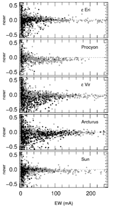
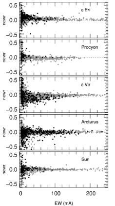
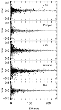
At the beginning of the calibration routine the s are distributed
as shown in Fig. 3
(in this and in the two following figures we only show the s of the elements
Fe and Ti for the sake of clarity).
After 100 iterations the distributions emerge as in
Fig. 3. Note that the dispersion of the points has decreased
and that the Fe lines (gray points) in Procyon, and the Ti lines (black
points) in Vir have an offset. The
offsets are due to the assumption of the wrong Fe and Ti abundances for these stars at the
beginning of the procedure. To continue with the s calibration we
must apply the second part of the calibration process, i.e., the abundance
correction, which is done manually. The negative offset of the Ti lines in
Vir indicates that the Ti lines are too strong, therefore, to match the observed
spectrum, the Ti abundance must be decreased.
Similarly, when the offset is positive, the abundance must be increased.
These evaluations and the consequent changes in abundance are done by observing the
distribution of the for lines for which the isolation degree parameter
is larger than 0.99 (which implies the selection of isolated lines alone) in order to guess the right
abundances from isolated lines. If no isolated lines are present, the
abundances remain [El/H]=[M/H].
The abundance correction is performed after the s calibration and
both are carried out many times until no more lines
are rejected by the calibration routine and the distributions
are centered on zero.
We want to spend a few more words on the abundance correction. The optimal
condition for the s calibration would be to have precise elemental
abundances for all the stars employed (as required by
equation (4))
so that the abundance correction would not be necessary.
Because at the time of this work precise abundances of these stars were not available,
in order fulfill the condition in equation (4)
as much as possible, we adopt the known
abundances, i.e., the Sun and the Arcturus abundances. For the
other stars (or elements) for which we do not have chemical abundances,
we adopted [El/H]=[M/H] and then followed the method described before
(i.e., observing the distribution of the s of the isolated lines of
an element and change its abundance to minimize the average of the absolute
values) whenever the adopted initial abundance was not satisfactory for this element.
In the case of the element Co on Arcturus, we decided to follow this method
and we adjusted its abundance to [Co/H]= dex because by using the
value [Co/H]= dex derived by Ramírez & Allende Prieto it was
not possible to minimize the absolute average values for all the stars.
We want to stress that the solar abundances were never
changed during the whole process. The Sun is synthesized with the
Grevesse & Sauval grevesse (1998) solar abundances and
these abundances must not be changed because this is the reference point
on which the whole calibration procedure is based. Without this reference
point no calibration is possible, otherwise the equation system
(4) would become underdetermined.
4.3 Setting the microturbulence
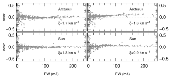
At the beginning of this work we tested several times the calibration routine in order to find the best way to follow. In some of these tests we adopted the microturbulence values reported in Jofré et al. jofre (2014), which are 1.2, 1.3, 1.8, 1.1, and 1.1 km s-1 for the Sun, Arcturus, Procyon, Eri, and Vir, respectively. With these values we could not find satisfactory results, which means that the s of the isolated Fe lines did not align close to the line for some of the stars, no matter what Fe abundance was adopted. Therefore, we decided to change the values interactively during the calibration process to minimize the absolute s values. The s values are sensitive to microturbulence and in Fig. 5 we show the difference in the s distributions observed by changing the microturbulence by 0.4 km s-1 (while all other parameters are fixed) for the Sun and Arcturus, with the best performing value in the lefthand panels. Our final best values are reported in Tab. 1.
4.4 The final line list
The whole calibration procedure described in the previous section is performed by applying alternatively the routine and the abundance correction iteratively until convergence of the abundances and until no more lines are removed by the routine. The process began with a line list of 8 947 lines. After the convergence, the final line list counts 4 643 lines. The s distribution of the final line list is shown in Fig. 3, while in Tab. 3 we report the abundances derived with the abundance correction procedure for the elements that we consider reliable (see Sec. 4.6 for further explanations). The final line list with the calibrated s is released together with the GCOG library.
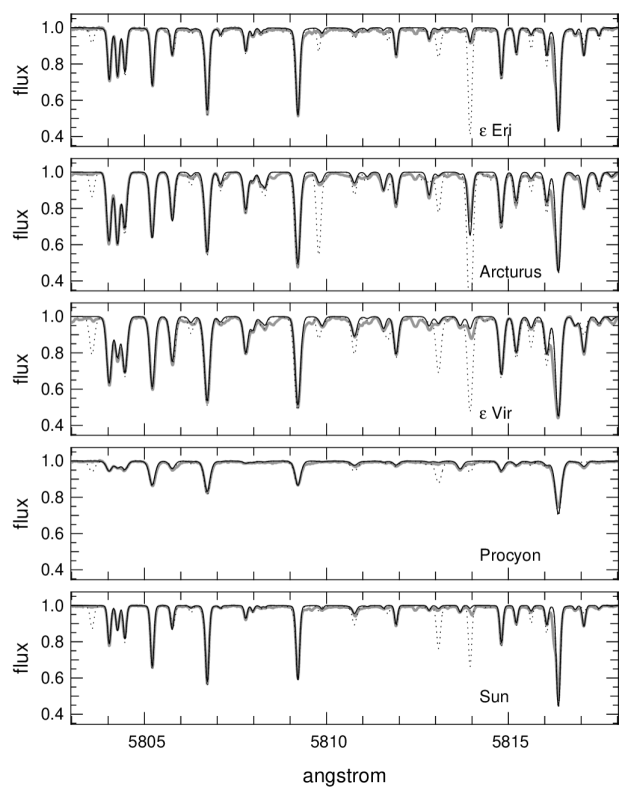
At the end of the calibration procedure we verified by eye inspection the good match between the synthetic and observed spectra over the whole wavelength range considered. In some cases there are unidentified absorption lines for which none of the lines given in the VALD database seems to match. These lines are neglected during the analysis performed by SP_Ace. We removed by hand some lines of the line list because were clearly erroneous (but not removed by the calibration routine because they lie under incorrectly fitted lines, like under the Ca triplet lines, for instance) or because their s were badly affected by unidentified lines. In Fig. 4 we compare part of the synthetic and the observed spectra before and after the s calibration. For this figure the synthesis was performed using the final abundances reported in Tab. 3, so that the differences between the spectra synthesized with the VALD s and the calibrated s are only due to the difference in s. Fig. 4 shows that the spectra synthesized with the new calibrated s match the observed spectra better than the ones synthesized with the VALD s.
4.5 Validation of the calibrated s
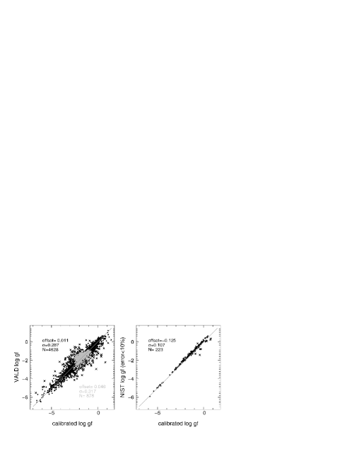
In Fig. 6 (left panel) we compare the original s of the VALD database with our final calibrated s for those lines that have mÅ in the solar spectrum. The residuals have an average offset of with a dispersion of (statistic computed excluding strong lines for which was calibrated by hand and after rejection of outliers with a 3 clipping). Because VALD is a database that collects data from several sources with different degrees of precision, we want to verify the robustness of our calibrated s comparing them with precise values. For this purpose, we accessed the NIST database (Kramida et al. nist, 2013) and select lines that have a precision better than 10% (0.04 in ) and mÅ on the solar spectrum. With these criteria we found 328 lines in common with our line list. After removing the lines with mÅ (for which we expect the largest calibrated errors) we are left with 223 lines belonging to the elemental species C I, N I, O I, Na I, Mg I, Si II, Sc I, Sc II, Ti I, V I, Cr I, Mn I, Fe I, and Co I. The comparison between the NIST and the calibrated s is shown in right panel of Fig. 6. The comparison with high precision s shows that our calibrated s have an offset of dex with a dispersion of 0.1 dex. The negative offsets say that our s are more negative than the corresponding NIST s. This can be due to several causes, which may be i) an inappropriate line profile of the synthetic spectra (the line profiles can vary for lines with different strengths and lines broadening parameters) ii) an inappropriate continuum normalization of the observed spectra, iii) neglected Non Local Thermodynamic Equilibrium (NLTE) and 3D effects, iv) errors in the stellar parameters adopted to synthesize the spectra. As a last remark, one may regard at the solar abundances adopted (Grevesse & Sauval grevesse, 1998) as the cause of the offset of our calibrated s. If these abundances (and in particular the Fe abundance, which has the higher number of lines represented in Fig. 6) were too high, the calibration would render s lower than expected. Some works, based on laboratory s, derived a solar iron abundance121212Here we define . of (ruffoni_ges, 2014, Ruffoni et al.; bergemann2012, 2012, Bergemann et al.). Since we adopted , this would explain part of the offset observed for our s.
4.6 On the accuracy of the calibrated s
Although we verified by eye the good match between the spectra synthesized
with our final line list and the observed spectra, this does not ensure the
good accuracy of the astrophysically calibrated s for all the lines of
the line list.
In fact, the spectra exhibit many blended features composed of many lines
that cannot be fully resolved, because for such blends the equation system
(4) is underdetermined. On the other hand, weak lines
(mÅ) are the ones more affected by imprecision of the continuum
placement or by blends. A difference in 0.5% of the normalized flux between
the synthetic and the observed spectra can look like a “good match” to
an eye inspection, but it leads to a very poor accuracy of the of a
line having an EW of a few mÅ. Another source of uncertainty comes from the abundance
correction procedure when the lines of one element are all weak in the Sun’ s
spectrum. With the Sun as reference point, when the lines are weak the
match with the synthetic spectrum is subject to the uncertainties discussed above,
so that the reference point becomes uncertain. For this reason,
the derived elemental abundances output by the code SP_Ace (in its
present version), are for those
species for which the number and strength of
lines are big enough for a good abundance estimation of the
five stars during the abundance correction process outlined in
Sec. 4.2. These elemental abundances are the ones
reported Tab. 3. The abundances of other elements are also
internally derived by SP_Ace but are used as “dummy” elements and
rejected at the end of the analysis.
There are further reasons why the calibrated s of some lines
may be not physically meaningful. We employed stellar atmosphere models
that are one-dimensional and the physical processes are assumed to take
place in Local Thermodynamic Equilibrium (LTE). This is an approximation that, in
some cases, is too rough to describe real stellar atmospheres. Some absorption lines
suffer of non-LTE effects, which can affect the observed EW.
Therefore, if we perform an astrophysical calibration of the s of
one of these lines under LTE assumptions, the calibrated value
can be significantly different from the real value (which expresses the
probability of the electronic transition) and the difference accounts for
the neglected non-LTE effect. This is not the right way to correct for non-LTE
effects and it may lead to systematic errors when stellar parameters
and the chemical abundances are derived.
During the s calibration and abundance correction procedure, we identified several
strong lines that cannot be correctly synthesized in our five standard
stars. The profiles of these synthetic lines have too strong (or too weak) wings
with respect to the observed lines in the spectra of the standard stars.
Some of these lines are reported in Tab. 4 with a
qualitative goodness of fit of the wings (and strength) between the synthetic and observed
lines. For some lines (such as most of the H I lines and the Na I doublet at
5890) we changed the s (and also the damping constants for
the Paschen H I lines) by hand in order to match the strength
of these lines in the solar spectrum. However, the match is often not satisfactory.
Most of the Mn I lines show a line width too narrow in synthetic spectra
with respect to the observed ones, and in the Sun synthetic spectrum these lines
are too strong at the core, although their EWs seem to be close to the observed ones.
The Mn I abundance is therefore rejected from the SP_Ace results.
All these discrepancies can be due to non-LTE effects, 3D effects, and
hyperfine splitting of the lines that we do not take into account in the present
work.
| wavelength | Sun | Arcturus | Procyon | Eri | Vir |
|---|---|---|---|---|---|
| 5269.537 Fe I | ok | + | ok | ok | + |
| 5328.039 Fe I | ok | + | ok | ok | + |
| 5371.489 Fe I | - | + | ok | – | ok |
| 5405.775 Fe I | ok | + | ok | ok | + |
| 5889.9510 Na I | ok | + | - | ok | - |
| 5895.9240 Na I | ok | + | + | ok | - |
| 8498.023 Ca II | ok | - | ok | ok | - |
| 8542.091 Ca II | ok | - | ok | - | |
| 8662.141 Ca II | ok | - | ok | - | |
| 8806.756 Mg I | ok | - | ok | ok | - |
Because these “poorly matching” lines can negatively affect the stellar parameter estimations, they
are rejected from the analysis performed by SP_Ace.
However, the fact that the spectra synthesized with our line list with
calibrated s match reasonably well131313The residuals between the
synthetic and the observed spectra have a standard deviation of
% of the normalized flux. the great majority of the spectral
range of our standard stars (which span a wide range in temperature and
gravity) and that most of the abundances derived
during the abundance correction process are close to the ones reported in
high-resolution studies (see Tab. 3), suggests that our line
list under LTE assumption can be employed to derive reliable stellar parameters and
chemical abundances in the and ranges covered by the
five calibration stars adopted in this work.
4.7 The molecular lines
In the previous sections we discussed mainly the atomic lines, although
molecular lines of several species are present in the wavelength ranges
considered. During the preparation of this work we did several tests
to verify whether a s calibration of atomic and molecular lines together
was possible. We found that i) the calibration is not always
possible, and ii) when it is possible, the calibrated s are
physically meaningless and can be only used as dummy values.
The first point applies to the wavelength range 5212-6860Å where the
very high number of molecular lines of the species CN, CH, MgH, and TiO
generate a forest of weak lines in cool star spectra that makes
the identification of the lines impossible and the equation system (4)
becomes underdetermined.
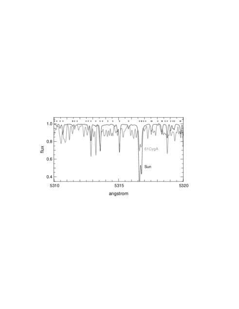
In Fig. 7 we compare the spectrum of the Sun (normalized by Hinkle et al.
hinkle, 2000, =5777 K, =4.44, [M/H]=0.0 dex) and 61CygA (normalized by
Blanco-Cuaresma et
al. blanco-cuaresma, 2014, =4374 K, =4.63, [M/H]= dex).
The forest of weak molecular lines in 61CygA is
so dense that it creates a “pseudo-continuum” that hides the real continuum
and prevents the correct estimation of the EWs of the atomic lines.
This convinced us that, at present, our method cannot calibrate s of
molecular lines in the interval 5212-6860Å.
Besides, to calibrate s of atomic lines we need spectra “free” of
molecular lines. Therefore we verified that the standard stars employed for the
calibration are not significantly affected by molecular lines.
We verified that this is true for dwarf stars having K
and for a giant star like Arcturus.
In the interval 8400-8924Å the second answer above applies:
here we can identify the CN lines and calibrate their s, but we strongly doubt
the accuracy of the calibration. When the original by Kurucz
are applied, the synthetic CN lines of Arcturus are far too strong
with respect to the observed ones. Molecular lines are known to be
prone to NLTE effects
(Hinkle & Lambert,hinkle_molecule, 1975; Schweitzer et al.
schweitzer, 2003; Plez, plez, 2008) and 3D effects (Ivanauskas
et al. ivanauskas, 2010), and their strengths may not be correctly
reproduced under 1D LTE assumption.
In order to match the strenghts of the CN lines observed on the Sun and on
Arcturus at the same time we needed to set the Arcturus C and N abundances
to [C/H]=[N/H]= dex, which lie between the atomic
abundances by Ramírez & Allende Prieto
ramirez (2011) who found [C/H]= dex and [N/H]= dex
and the ones of Smith et al. smith (2013) who found [C/H]= dex and
[N/H]= dex.
We believe that Arcturus’ low C and N abundances found
by us merely counterbalance the 3D NLTE effects that we could not take in account.
Thus, the CN lines
in the wavelength interval 8400-8924Å are employed by SP_Ace as “dummy”
lines and the results are rejected after the estimation process.
5 The Equivalent Widths (EW) library
We built the EW library using the driver ewfind of the code MOOG,
which computes the expected EW of the absorption lines for a given stellar
atmosphere model. We employed the atmosphere models grid ATLAS9
by Castelli & Kurucz castelli (2003) updated to the
2012 version. The Castelli & Kurucz grid has steps
in stellar parameters (500 K in , 0.5 in , and 0.5 in [M/H]) that
are too wide for our needs. We linearly interpolated the models to obtain a
finer grid with steps of 200K in , 0.4 in , and 0.2 dex in [M/H] and
covering the ranges 3600-7400 K in , 0.2 to 5.4 in 141414The
Castelli & Kurucz grid has a upper limit of 5.0. To explore the
space around this limit (necessary for a cool dwarf stars that can
have , for instance) SP_Ace needs to construct spectral models
with 5.0. Thus, we extended the EW library to =5.4 by
computing the EW of the lines with a linear extrapolation.,
and to dex in [M/H]. In the following we always refers to this grid.
The microturbulence assigned to each atmosphere model is computed
as a function of and . This function is described in
Appendix A.
Note that in Sec. 2 we defined
the GCOG as a function of
the three variables , , and [El/H] (and not [M/H]).
However, to construct the EW library we need the metallicity [M/H] of the atmosphere
model. In fact, besides the , , and the abundance [El/H], the EW of a line
also depends on the opacity of the stellar atmosphere in which the line
forms, which is driven by atmospheric metallicity [M/H]. This means that to compute the GCOG
of a line we must also define the metallicity of the atmosphere model,
making (in this specific case) the GCOG a function of four variables.
Therefore, we define the stellar parameter grid in the three dimensions ,
, and [M/H] plus a fourth dimension that accounts for the relative abundance
[El/M].
To construct the EW library, for every point of the grid and every line of our line list we computed
the EW of the lines at 6 different abundance enhancements with respect to
the nominal metallicity of the atmosphere model, that means (for the generic element
El) [El/M], , , , , and . These 6 points
belong to the COG of the lines for every grid point.
The EW library so constructed contains the EWs of the lines synthesized as they were
isolated. Because SP_Ace constructs the spectrum model by summing up the absorption lines
with given EWs, the spectrum model is realistic if the lines are
isolated or, in case of blends, if the EWs of the involved lines are small
(i.e., weak line approximation).
Because these conditions are not always satisfied in a real spectrum,
in the following we discuss how to remove the weak line approximation.
5.1 The weak line approximation problem
Consider the case of two or more lines that are instrumentally blended but
physically isolated in a spectrum. We can write
| (3) |
where is the total EW of the blended feature, are the EWs of
the lines computed as isolated, and the number of
lines considered.
Consider now the same lines as before, but now they are physically blended.
If the lines have small EWs, then equation (3) is still
(approximately) valid because their line opacity is
small and does not affect the local opacity significantly.
This is what we call weak line approximation. Under these conditions
we can use the of the lines contained in
the EW library and,
assuming a line profile, subtract the lines from a normalized continuum to obtain a
spectrum model which approximates the synthetic spectrum well.
Unfortunately, the weak line approximation can rarely be applied because
strong and broad absorption lines are common in real spectra.
In case of strong lines, equation (3) is not true anymore,
because the opacities of the lines diminish reciprocally the flux absorbed by them,
and equation (3) becomes the inequality
| (4) |
where indicates the total equivalent width of the blend and is as in equation (3). In this case, by summing up the of the lines contained in the EW library would render a spectrum model where the blends are too strong with respect to the synthetic ones. This is shown in Fig. 8 where a blended feature constructed using equation (3) (dotted line) with EWs from the EW library turns out to be much stronger than the of the feature synthesized by MOOG (black line).

To correctly
reproduce the blend, the of the EW library
must be corrected for the opacity of the neighboring lines, so that the
EWs employed to construct the spectrum model are smaller than the
corresponding isolated lines.
These corrected quantities that we call “equivalent widths corrected
for the opacity of the neigbouring lines” () are smaller than
and satisfy the equation
| (5) |
The quantity cannot be computed with MOOG. In fact, to know the quantity we need to compute the fraction of the contribution function due to each absorber present in the stellar atmosphere (continuum, atoms, molecule) that form the blend. These fractions of the contribution function are not usually computed by spectral synthesis codes. This information is lost when the spectral synthesis code computes the total opacity at wavelength by summing up the opacities of all the absorbers to obtain the optical depth . The way to compute the fraction of the contribution function is discussed in Sec. 5.2 and, although a rigorous solution was found it cannot be used to correct the EWs of the library. An approximate solution must be adopted and this is outlined in Sec. 5.3.
5.2 Separating the contributions of each absorber
In the attempt to obtain the quantity , we tackled and solved the problem to compute the fractions of the contribution function due to each absorber individually. Unfortunately, the result turned out to be inapplicable for our purpose: we can compute the flux absorbed by each absorber but this cannot be written in terms of EW. To explain this apparent paradox, we here outline the general result and point the reader to Appendix B for the full detailed solution. Although the problem concerns blends, the simple case of one isolated line is also illustrative for multiple absorbers like in blends. In fact, in the case of one line the opacity is due to two absorbers: the continuum and the line. In Fig. 9 we show an absorption line (gray solid line) and the continuum in absence of the absorption line (dotted line). The EW of this line, as commonly defined, is represented by the area between the gray and the dotted line. In this way, the EW does not represent the total flux absorbed by the line, because the continuum (dotted line) has been computed in absence of the line, i.e. the opacity of the line has been neglected. When the line opacity is taken in account, the continuum level is higher (the dashed line of Fig. 9) because it absorbs less radiation. In fact, when the line is present, its opacity diminishes the intensity of the radiation and the continuum absorber is left with less radiation to absorb. Therefore, the real flux absorbed by the line is represented by the area included between the gray and the dashed lines of Fig. 9, which is much bigger than the EW as usually defined. This proves that, although we can precisely determine the real quantity of flux absorbed by a line (in a synthetic spectrum), we still miss the solution of our problem. In fact, to reconstruct a spectrum model by summing up the absorbed fluxes we need to consider the continuum level at any wavelength. At the stage of development of our work, the variation of the continuum level as function of the strength of the lines looks too complicated to be implemented. Therefore we must follow another method to approximate the quantities and apply equation (5) to construct the spectrum models.


5.3 Approximated correction for the opacity of the neighbor lines
The method to approximate the quantity is based on the idea that when
the first derivative of the COG (expressed as EW as function of abundance)
inside a blend is small this means that its contribution to the absorbed flux
(i.e., the EW) is small too, similarly to what happens to the isolated
line. The method, outlined in the following example, makes use of
EWs of synthesized isolated lines and blended features.
The EWs of isolated lines are computed with the MOOG driver ewfind
which numerically intergrates the depression of the synthetic line with
respect to the continuum. Because this driver does not handle more than one
line per time, to compute the EW of blends we need to synthesize the blend
and numerically integrate the depression151515For a faster procedure we
modified the driver ewfind to make it handle more than one line per
time..
Consider one line in a blend composed of two (or more) lines indexed with . The lines belong to different elements . By using MOOG we compute the equivalent widths EWs of the lines as isolated for 6 different abundances [/M]=, , 0.0, +0.2, +0.4, +0.6 dex so that we have six points of the COG of the line (we call it COG). Similarly, for every line we synthesize the whole blend and we measure the total equivalent width of the blend . This is done by synthesizing the blend in which all the lines have constant [/M]=0.0 but for the -th line which assumes six different abundances [/M]. The six EWs of the blend so obtained represent the COG of the -th line in the blend (we call them COG). If the opacity of one line is not affected by the other line, then COG=COG, otherwise COGCOG. In particular, if the first derivative of COG is smaller than the one of COG, it means that the contribution of the -th line to the absorbed flux of the blend (this is the quantity we look for) is smaller than the one absorbed when the -th line is isolated. Thus, the quantity COG can be used to approximate as follows:
-
1.
Compute the first derivatives of the curves-of-growth and .
-
2.
Perform a first correction of as follows
-
3.
Under the assumption that the ratio of between the lines is conserved in the blend, the contribution to the absorbed flux of the -th line in the blend is approximated as
In the general case of a blend of lines and elements with , there
are two or more lines that belong to the same element . In this case, the
strengths of the lines would change together when we change the
abundance [/M] during the synthesis of the blend, and this must be avoided
in order to evaluate the COG of the target line.
This problem is solved by changing
the (and not the abundance) of the line, so that the target line is
the only line the strength of which changes in the blend.
The corrected values are computed for all the EWs contained in
the EW library considering any line closer than Å to the target line. Fig. 8 shows the improvement
obtained for a blend when the corrected values s are used to construct the spectrum model
(gray solid line) with respect to the model constructed with EWs (dotted
line).
The limit of 0.5Å is satisfactory for most of the lines. For a few intense
and broad lines (for instance, the Ti II at 5226.538Å), which can affect lines
farther than 0.5Å, a larger limit would be necessary. At this stage of
development, SP_Ace neglects these lines during the analysis.

6 The General Curve-Of-Growth (GCOG) library
The COG of a line is a function that gives the EW of a line as a function of the abundance of the element the line belongs to. This function can be recovered from the EW library where, for each absorption line, we stored six points of the COG between the [El/M] values and dex in steps of 0.2 dex. The EW library also contains the EWs that the lines assume over a grid spanning a wide range in the stellar parameters , , and [M/H]. Because the EW of a line changes not only as a function of the abundance but also as a function of and , we extend the concept of COG. We call General Curve-of-Growth (GCOG) the function that describes the EW of a line as function of the variables , , and [El/H], where [El/H] represents the abundance of the generic element El the line belongs to (see Fig. 10). Unfortunately the GCOG has no analytical form, therefore, to obtain the EW of a line we must approximate the GCOG with a polynomial function in the parameter space. In principle the GCOG has a three dimensional domain (, , [El/H]). As already reported in Sec.5, because we rely on a grid of stellar atmosphere models the opacity of which depends on [M/H], we must construct the polynomials in a four-dimensional space (, , [M/H], [El/M]). We refer to these functions as “polynomial GCOGs”, and they are constructed to approximate the GCOG of the lines. Thanks to the polynomial GCOGs, SP_Ace can compute the expected EW of any line at any point of the parameter space (, , [M/H], [El/H]) removing in this way the discontinuity of the grid in the EW library.
6.1 The polynomial GCOGs
We fit a polynomial GCOG for every absorption line in the parameter space.
Because of the difficulties in fitting a
function over points covering the whole parameter space, the polynomial
GCOGs fit the EWs that the line assumes over a limited stellar parameter
interval surrounding the points of the grid. The width of this interval is 800 K in , 1.6 in ,
0.8 dex in [M/H], and 1.0 dex in [El/M], which includes five grid points for the
first three dimensions and six for the last dimension.
For instance, for the grid
point =4200 K, =1.4, and [M/H]=0.0 the polynomial GCOG fits the EWs
that the line has at =3800, 4000, 4200, 4400, and 4600 K, =0.6, 1.0,
1.4, 1.8, and 2.2, [M/H]=, , 0.0, , and dex, and the six
abundance points [El/M]=, , 0.0, , , and dex
(Fig. 11). In total, every polynomial GCOG
fits 750 EWs. The polynomial GCOG function has the form
| (6) |
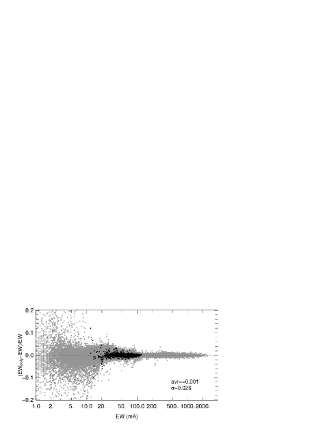
So defined, the polynomial GCOG has 70 coefficients that are computed by using a minimization routine that minimizes the between the polynomial and the given EWs. The residuals between the (given by the polynomial GCOG) and the EWs of the library are shown in Fig. 12. The residuals are on average 2.6% of the expected EW, which is equivalent to an error of dex in chemical abundance. Fig. 11 shows the polynomial GCOG of 50 absorption lines compared with the expected EW plotted as a function of , , [M/H], and abundance [El/M].
7 The SP_Ace code
In the following we outline the main structure of the code. This is not intended
to be a user manual. A detailed tutorial on how to use SP_Ace and the full
description of the available functionalities of the code is provided
together with the code.
The SP_Ace code is written in FORTRAN95. It processes one spectrum per
run. The observed spectrum must be wavelength calibrated, continuum
normalized and radial velocity corrected.
When launched, SP_Ace reads the parameter file that must include the name
of the spectrum to process, the address of the GCOG library, a first guess
of the FWHM, and other optional settings.
In the following we
outline the algorithm that summarized the SP_Ace analysis procedure
specifying the most important routines that we explain later.
This algorithm carries out the following steps:
-
1.
Upload the observed spectrum.
-
2.
Make a first rough estimation of the stellar parameters , , and [M/H]. (This is performed by the “starting point routine”.)
-
3.
Find the closest grid point to the estimated , , and [M/H] and upload the corresponding polynomial GCOG.
-
4.
Derive , , and [M/H]. (This is performed by the TGM routine.)
-
5.
Find the closest grid point to the derived , , and [M/H]. If it is different from the previous grid point, then upload the polynomial GCOG of the new grid point and go to step 4, otherwise continue.
-
6.
Re-normalize the observed spectrum. (This is performed by the re-normalization routine.)
-
7.
Derive , , [M/H] from the re-normalized spectrum. (This is performed by the TGM routine.)
-
8.
Find the closest grid point to the estimated , , and [M/H]. If it is different from the previous grid point, then upload the polynomial GCOG of the new grid point and go to step 6, otherwise continue.
-
9.
Derive the chemical abundances [El/M]. (This is performed by the ABD routine.)
-
10.
Go to step 6 and repeat until convergence.
-
11.
Derive the confidence limits for , , [M/H], and [El/M] (optional)
-
12.
End the process and write out the results.
Every step is composed of routines and sub-routines. The
most important ones are described in the following.
These algorithm can be executed with or without step 10.
This is controlled by the keyword ABD_loop (abundance loop) that can be
used by SP_Ace. When ABD_loop is switched on, step 10 is executed,
otherwise it is skipped.
The two settings show significant differences when run on real
and synthetic spectra. This is discussed in Sec.8.
7.1 The “make model” routine
To derive the stellar parameters and the chemical abundances,
SP_Ace constructs several spectrum models and compares them to the observed spectrum,
looking for the model that renders the minimum .
The routine that constructs the model (called the “make model” routine) is
therefore particularly important and it follows this algorithm:
-
1.
Set the initial spectrum model with the same number of pixels and wavelengths of the observed spectrum and initial flux normalized to one. We call it the “working model”.
-
2.
Consider the stellar parameter with which the model must be constructed.
-
3.
Consider the first absorption line of the line list.
-
4.
Compute the of the absorption line by using its polynomial GCOG.
-
5.
Compute the strength of the line profile at every pixel around the center of the line and subtract it from the working model. The result is the new working model.
-
6.
Consider the next line and go to step 4 until the last line has been reproduced.
The line profile adopted is a Voigt function approximated with the implementation by McLean et al. mclean (1994). We modified this implementation so that the line profile becomes broader as a function of and EW with a law that can be different for some special lines (for instance, lines with large damping constants). For a detailed description of the line profile adopted we refer the reader to Appendix C.
7.2 The “starting point” routine
This routine finds the first rough estimation of the stellar parameters. It uses the “TGM routine” outlined in the next section, with the difference that the polynomial GCOG employed has been computed not over a small volume of the parameter space (as explained in Sec. 6.1) but over the whole parameter space. This polynomial GCOG has larger errors with respect to the other polynomials contained in the GCOG library, but it permits a rough and fast estimation of the parameters, which is used as starting point by the next TGM routine.
7.3 The “TGM routine”
This part of the code is responsible for deriving the stellar parameters.
It employs the Levenberg-Marquadt method to minimize the between
the models and the observed spectrum in the parameter space (,
, [M/H]). At the fourth
step of the main algorithm, the TGM routine uses the observed spectrum as
provided by the user, while at the seventh step it uses the observed spectrum
after the re-normalization (explained in section 7.4).
Because the polynomial GCOGs were computed over an
interval of stellar parameters that covers 800 K in , 1.6 in , and
0.8 dex in [M/H] (see Sec.6.1) centered on a grid point (we
call it the “central point”), its reliability decreases with the distance
from the central point.
When the stellar parameters given by the TGM routine are close to a grid
point that is not the central point, the TGM routine stops,
uploads the polynomial GCOG for this new grid point, and repeats.
In this way the routine always finds the minimum close to the
central point, where the EWs provided by the polynomial GCOG are the most
reliable.
For some spectra (e.g., spectra with very low S/N, spectra of very cool/very
hot stars, or spectra of stars with high rotational velocity )
the TGM routine may try to move beyond the extension of the GCOG library. In
this case SP_Ace writes a warning message and exits with no results.
Apart from the stellar parameters, the TGM routine also estimates two other
parameters: the radial velocity and the FWHM of the instrumental profile.
Because SP_Ace only processes radial-velocity-corrected spectra, the radial
velocity estimation of SP_Ace is not a real measurement, but it is an internal setting
to improve the match between the model spectrum and the observed spectrum.
Usually this quantity amounts to a small fraction of FWHM.
Similarly, SP_Ace searches for the FWHM that matches best the instrumental
profile.
The optimization of the FWHM gives to SP_Ace some flexibility in estimating
the stellar parameters for stars with a rotational velocity different
from zero. However, the Voigt profile adopted by
SP_Ace cannot properly fit the shape of the lines of stars with high ,
and the limit beyond which the line profile becomes inadequate depends
on the spectral resolution. This limit is higher for low-resolution spectra
in which the instrumental line profile dominates over the physical profile of
the line.
7.4 The re-normalization routine
As stressed before, SP_Ace can only handle flux-normalized spectra. However, it can perform a re-normalization to adjust the continuum level. This operation may be unnecessary for high-resolution and high-S/N spectra, where the continuum is clearly detectable and a normalization done with the commonly used IRAF task continuum is usually satisfactory. For low-resolution, low-S/N spectra, and in particular for spectra crowded of lines, the continuum cannot be clearly identified. At low resolution, the lines are instrumentally blended and they create a pseudo-continuum that can lie under the real continuum. In this case, the IRAF task continuum cannot correctly estimate the continuum and renders a too low continuum level, leading to an underestimation of the metallicity (as well as the other stellar parameters, since they are correlated). As an example, in Fig. 14 we show a low- and a high-resolution spectrum (synthetic) of a high-metallicity star, and the result of the continuum normalization performed with the IRAF task continuum, using a spline function and low_rej=1 and high_rej=4, settings that take the presence of absorption lines in the spectra in account.


Because of the instrumental blend of the lines, the low-resolution spectrum
suffers of a too low continuum estimation and its normalized flux is too high.
When the same continuum settings are used for very low S/N spectra
the normalized spectra suffer the opposite problem:
the noise dominates the spectrum and the flux distribution becomes nearly
symmetric with respect to the continuum.
(This commonly happens in spectroscopic surveys when the number of spectra
to normalize is big and the parameters of the task continuum
cannot be set by hand for every spectrum).
In this case, the settings low_rej=1
and high_rej=4 are not appropriate and cause a too high estimated continuum
(and an overestimation of the metallicity).
To fix this problem, SP_Ace re-normalizes the observed spectrum.
In the following, indicates the normalized flux of the
observed spectrum and indicates the normalized flux of the spectrum
model. The re-normalization routine works as follows:
-
1.
Consider the -th pixel at wavelength and the pixels for which
-
2.
Compute the average of the observed flux , the average of the residuals and their standard deviation of the pixels defined before.
-
3.
From the set of pixels defined in step 1, reject the pixels with . The new set of pixels has now number of pixels.
-
4.
With the new set of pixels, compute the new average of the observed flux , the average of the model .
-
5.
Compute the continuum level at the -th pixel as
-
6.
Re-normalize the -th pixel of the observed spectrum as
-
7.
Move to the next -th pixel and go to step 1 until all the pixels have been processed.
7.5 The ABD routine
The routine to derive the chemical abundances (called “the ABD routine”) works similarly as the TGM routine. The ABD routine is run after the TGM routine. The abundances [El/M] are varied by a minimization routine until the between the model and the observed spectrum is minimized.
7.6 Internal errors estimation
SP_Ace can estimate the expected errors for the parameters , , and
the chemical abundances [El/M]. The routine dedicated to this task finds the
confidence limits of the stellar parameters intended as the region of the parameter
space that contains a certain percentage of the probability distribution
function (Press et al. nr, 1992). If we want to determine the extension of the region
that has a 68% of probability to include the resulting parameter (say
best) with the lowest (), this region is an interval
that has an upper and a lower limit up
and low with . Because
the stellar parameters are correlated, the confidence limits of one
parameter are a function of the others, so that the upper and lower confidence limits of
as a function of correspond to the largest and smallest values
of with where
depends on the number of degrees of freedom (Press et al. nr, 1992).
The higher the number of degrees of freedom, the larger the confidence limits.
Because the determination of
these limits is computationally expensive, we limited this determination
to three variables, namely , , and [M/H] for these three stellar
parameters, and , , and [El/M] for the
chemical abundance of the generic element El. This means that we determine the upper and
lower limits of any parameter at .
These confidence limits must be considered as internal errors (therefore smaller than the real
errors) because they do not take external errors into account like
the mismatch between the atmosphere model and the real stellar atmosphere,
uncertainties in the atomic transition probability, in the continuum
placements and other uncertainties in the spectrum model construction.
The error estimation is an option left to the user because it is computationally
expensive: when done, it can easily double (or more) the time required to process
the same spectrum without error estimation.
7.7 Output results
At the end of the process, SP_Ace writes four output files. One file called “space_TGM_ABD.dat” contains the resulting stellar parameters , , and chemical abundances with their confidence intervals, the number of lines measured, and a few other parameters like the of the best matching spectrum model, internal RV and FWHM. The second output file called “space_model.dat” contains a table the columns of which correspond to i) the pixel wavelength of the observed spectrum, ii) the flux of the observed spectrum, iii) the flux of the observed spectrum after re-normalization, iv) the flux of the best matching model, v) the continuum level adopted for the re-normalization, and vi) the weights of the pixels (rejected pixels have weight=0). The third output file “space_ew_meas.txt” contains the EW employed by SP_Ace to construct the model. We want to stress that these are not the EWs of the absorption lines but merely the (EW corrected for the opacity of the neighboring lines) computed from the polynomial GCOG during the construction of the best matching model. The fourth output file “space_msg.txt” contains the warning messages generated when something goes wrong during the analysis.
| mock | age | [Fe/H] range | C , N , O | Mg | Al , Si , Ca , Ti | other elements | ||||
| population | (Gyr) | (dex) | ||||||||
| thin disk stars | 5 | [Fe/H] | 0.0 | 0.0 | 0.0 | 0.0 | 0.0 | 0.0 | 0.0 | 0.0 |
| [Fe/H] | 0.0 | 0.0 | 0.0 | 0.0 | 0.0 | |||||
| halo/thick disk stars | 10 | [Fe/H] | 0.0 | 0.0 | ||||||
| [Fe/H] | 0.0 | 0.0 | ||||||||
| accreted stars | 10 | [Fe/H] | 0.0 | 0.0 | 0.0 | 0.0 | 0.0 | 0.0 | 0.0 | 0.0 |
8 Validation
To establish the precision and accuracy of the stellar parameters and
chemical abundances derived by SP_Ace, we run the code on several sets of
synthetic and real spectra with well known parameters and compare them with
the parameters derived with SP_Ace. We test SP_Ace on the wavelength ranges
5212-6270Å and 6310-6900Å, which avoids the range 6270-6310Å where
the presence of telluric lines can affect the analysis. The tests are
performed on spectra with spectral resolution between 2 000 and
20 000161616At R20 000 the line profile implemented in SP_Ace is expected to work best. See Appendix C for a short discussion
on the accuracy of the line profile as a function of the spectral
resolution..
Before the presentation of these tests, we illustrate and discuss the
accuracy with which SP_Ace constructs the spectrum models (i.e. how close these
models match the synthetic spectra from which they are derived).
8.1 Spectrum models accuracy
In Sec. 7.1 we outlined the algorithm that constructs the
spectrum model which must be compared with the observed spectrum. Our goal
was to make a spectrum model that looks as close as possible to a synthetic spectrum.
To evaluate the accuracy with which the spectrum models constructed by
SP_Ace match the corresponding synthetic spectra, we synthesized two
spectra and
compared them with the corresponding spectrum models constructed with the
same stellar parameters. The goodness of the match illustrates the precision with
which the strength of the lines (encoded in the EW library first, and then
in the GCOG library) and the line profile adopted, can reproduce a realistic
spectrum model. We chose to synthesize the spectra of a dwarf star
(=5800 K, =4.2, [M/H]=0.0 dex) and of a giant star (=4200 K, =1.4, and
[M/H]=0.0 dex) degraded to a spectral resolution of R=12 000171717The
accuracy with which the model spectra match the synthetic ones can change
with spectral resolution and stellar parameters. For the sake of brevity, we
only present here two spectra as exemplary cases.. The
relatively high metallicity adopted generates spectra rich in lines, allowing
us to verify how well SP_Ace can reproduce blended features (more numerous in
spectra of giants) and
how good it fits the profile of strong lines (usually broader in dwarf stars).
In the case of blended features we test the correction for the opacity of
the neighboring lines applied to the EW library (Sec. 5.3),
for isolated strong and weak lines we verify the goodness of the Voigt profile adopted (described in
Appendix C). In general, any line is affected by the precision
with which the polynomial GCOGs represent the expected EWs.
The comparison between models and synthetic spectra is shown in
Fig. 15. The top panel of the figure shows that the
normalized flux of the models differs by no more than 1% for most of the
wavelengths, with a general standard deviation of 0.2% and 0.6%
for the dwarf and the giant, respectively. This statistic was computed after
the rejection of the gray shaded areas, which were rejected during the
analysis because in the case of real spectra they are affected by unidentified lines, lines with NLTE effects, or
lines for which the correction for the opacity of the neighboring lines is not
satisfactory (see last paragraph of Sec. 5.3).
Although not perfect, the spectral models match the corresponding synthetic
spectra with a satisfactory degree of accuracy .
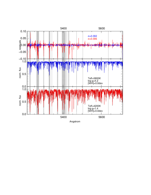
8.2 Tests on synthetic spectra
To verify the ability of SP_Ace to distinguish the stellar parameters and chemical abundances of different Milky Way stellar populations of different ages, metallicity, and evolutionary stages, we synthesized the spectra of three mock stellar populations with characteristics that mimic the thin disk stars, the halo/thick disk stars, and accreted stars with non-enhanced abundances (a dwarf galaxy accreted by the Milky Way, for instance). All the synthetic spectra were synthesized with MOOG, adopting the final line list described in Sec. 4.4 and atmosphere models from the grid ATLAS9 by Castelli & Kurucz castelli (2003) (updated to the 2012 version) linearly interpolated to the wanted stellar parameters.
8.2.1 Construction of the synthetic mock populations
We construct a mock sample for a total number of 1200 spectra for the three
populations (300, 600, and 300 spectra for
the thin, halo/thick, and accreted populations, respectively),
randomly chosen from the PARSEC isochrones (Bressan et al.
bressan, 2012 complemented by Chen et al. chen_bressan, 2015)
to cover the stellar parameter range 3600 to 7500K in , 0.2 to 5.0 in
, and to dex in [Fe/H].
In this way, the mock sample covers uniformly the chosen isochrones.
Their chemical abundances were chosen with the following characteristics:
-
•
mock thin disk stars: they cover the iron abundance ranges and their and were taken from isochrones with an age of 5Gyr. Their -elements enhancement [El/Fe] becomes progressively higher for lower [Fe/H]. (In the next plots this population is represented by blue points.)
-
•
mock halo/thick disk stars: they cover the iron abundance ranges and their and were taken from the isochrones with an age of 10Gyr. Their -element enhancement [El/Fe] becomes progressively higher for lower [Fe/H] down to dex, and stays constantly high () for dex. (In the next plots this population is represented by red crosses.)
-
•
mock accreted stars: they cover the iron abundance ranges and their and were adopted from isochrones of an age of 10Gyr. Their -element enhancements [El/Fe] are equal to zero. (In the next plots this population is represented by dark green triangles.)

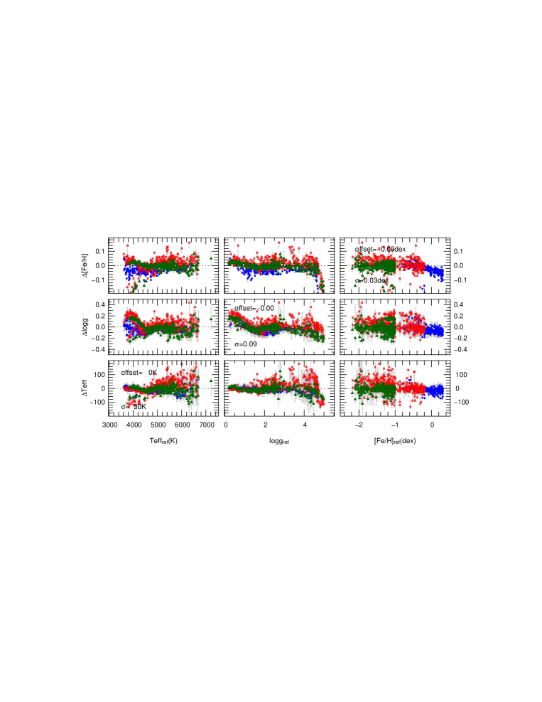

More precisely, the abundance of the generic element follows a linear law which can be expressed as , where and have different values for different [Fe/H] intervals and elements. The exact and values for each element are listed in Tab. 5. The distributions of these populations in and are shown in the left panel of Fig. 16. The samples were degraded to resolutions of R=20 000, 12 000, 5 000, and 2 000 and to signal-to-noise ratios of S/N=100, 50, 30, and 20 (by adding Poissonian noise) for a total amount of 19 200 spectra. The stellar parameters and abundances of these spectra were derived with SP_Ace and compared with the expected ones. The measurements were performed with the keyword ABD_loop on. We switched off the internal re-normalization to evaluate the goodness of the GCOG library to provide the right EW of the lines and the ability of SP_Ace to reproduce the correct line profile of the absorption lines.

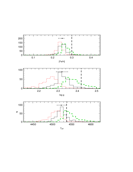
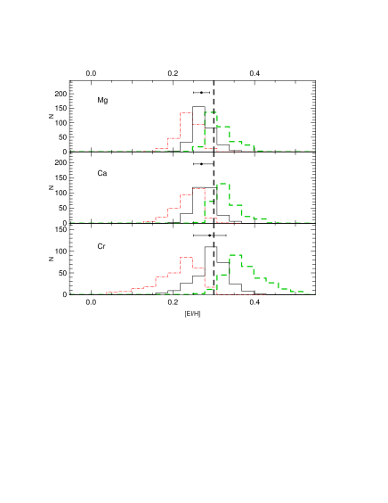
8.2.2 Results
We run SP_Ace on the sets of synthetic spectra just outlined. For the sake of brevity, we only report here the representative case of R=12 000 and S/N=100. In Fig. 16 we show the distribution in and of the synthetic spectra (left panel) in comparison with the same parameters derived by SP_Ace (right panel). The and derived by SP_Ace follow closely the isochrones for all three synthetic populations. In Fig. 18 we show the residuals between the derived and reference values as a function of the reference stellar parameters while in Fig. 18 we report the distribution of the chemical abundances in the chemical plane for nine elements derived from the same spectra.
8.2.3 Errors estimation in synthetic spectra
In the panels of Fig. 18 we report the dispersions of the measurements around the expected values of , , and [M/H], while the confidence interval of the single measurements (computed as explained in Sec. 7.6) are shown with the light gray errorbars. The errorbars in Fig. 18 are often smaller than the dispersion of the residuals, which suggests an underestimation of the errors. This is summarized in Fig. 19 where the overall dispersion of the residuals for the stellar parameters (derived minus reference, black symbols) are compared with the half-width of the confidence intervals (gray symbols) for different resolutions and S/Ns. The black and gray symbols are closer where the stochastic noise dominates, i.e., at low S/N, while for high S/N the confidence intervals always underestimate the stellar parameter dispersions. The reason can be guessed from Fig. 18: the overall dispersion is inflated by the presence of systematic errors in , , and [Fe/H] for which the computed confidence intervals cannot account. The latter can only account for the stochastic errors. We proved the last statement by generating 100 Monte Carlo realizations of a few synthetic spectra, derived their stellar parameters and chemical abundances, and compared them with the confidence intervals computed by SP_Ace. The distributions of the parameters and the confidence intervals obtained with this test show that the confidence intervals only account for the stochastic noise and fail to recognize the systematic errors when present (the shift between the average of the black histogram and the expected value represented with a black dashed line in Fig. 20). The chemical abundances recovered by SP_Ace for the three mock samples (see Fig. 18) are accurate and follow the expected sequences traced by the colored solid lines. No particular systematic error is visible and the errorbars appear to be a good representation of the dispersion around the expected value. This is supported by the statistic obtained from the 100 Monte Carlo realizations cited before and illustrated in Fig. 21. A further discussion of the systematics errors seen in this section can be found in Sec. 8.5.
8.3 Tests on real spectra
We employed sets of publicly available spectra like the ELODIE spectral library (Prugniel et al. prugniel, 2007), the spectra of the benchmark stars (Jofré et al. jofre, 2014), and the spectra of the S4N catalogue (Allende Prieto et al. allende, 2004). For the ELODIE spectra we selected those spectra for which the authors report literature stellar parameters flagged as being of good and excellent quality (quality flags “3” and “4”) to be compared with the stellar parameters derived by SP_Ace. For the benchmark and S4N stars we compare our results with the high quality stellar parameters provided by Jofré et al. and Allende Prieto et al., respectively. All these spectra have high spectral resolution (60 000) and high S/N. To test SP_Ace on spectra of lower resolution and S/N, we degraded the spectra to resolutions of R=20 000, 12 000, 5 000, and 2 000 and to S/N=100, 50, 30, and 20 by adding artificial Poissonian noise181818Many of these spectra have S/N that are not high (S/N60-100) so that by adding artificial noise the final S/N is actually lower than the nominal one.. Although the original spectra were already normalized, we re-normalized them after degrading them with the IRAF task continuum in order to simulate the continuum obtained when these spectra are normalized at their nominal spectral resolution. Then, the spectra were processed with SP_Ace and the derived stellar parameters compared with the reference values. For the sake of brevity, we only report here the representative case of R=12 000 and S/N=100. We measured the spectra with the ABD_loop keyword in the wavelength range 5212-6270Å and 6310-6900Å to avoid the telluric lines in the range 6270-6310Å that may degrade the quality of the measurements. In this case we switched on the internal re-normalization as usually done for spectra for which the continuum level must be refined.
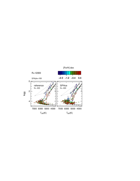
8.3.1 Results
The distributions on the and plane of the reference parameters and the derived parameters with SP_Ace are shown in the left and right panels of Fig.22, respectively. The derived parameters appear to follow fairly well the isochrones. In Fig. 24 the residuals between the derived and expected values as a function of the reference stellar parameters show small residuals in all the panels, except for the middle right panel, which reveals a systematically low with lower [Fe/H]. This feature is discussed in Sec.8.5.1.
8.3.2 Error estimation in real spectra
Because for real spectra we do not have exact stellar parameters but estimations from high resolution spectra, our evaluation of the errors relies on the dispersion of the residuals between the parameters derived by SP_Ace and the high resolution parameters that we use as reference. This is summarized in Fig. 26 for different resolutions and S/N ratios. Because the reference parameters also suffer from errors, the dispersions reported in Fig. 26 are actually an overestimation of the SP_Ace errors because they result from the quadratic sum of the reference errors plus the SP_Ace errors191919 The reference values of the S4N and the benchmark stars’ gravity was derived from parallaxes. Therefore we expect that, being such estimation usually much smaller than the ones derived from spectra, for these stars the SP_Ace errors are the major contributors to the dispersion of the redisuals.. For the individual elements, Fig. 24 shows nine relative abundances derived from the same spectra. For these quantities reference values can be only found for the S4N spectra, for which we have seven elements in common. The comparison between derived and reference abundances is reported in Fig. 25.
8.4 Measure of the whole ELODIE spectral library
We derived stellar parameters and chemical abundances for the whole ELODIE spectral library at a resolution of R=12 000 and S/N=100. SP_Ace provided results for 1386 spectra (out of 1959 spectra of the library) while it did not converge for those spectra which stellar parameters are beyond the stellar parameter volume covered by the GCOG library. The high number of stars provided by the full ELODIE library gives a more robust statistic with respect to the previous test. The derived parameters are reported in appendix D, Tabs. 6, 7, and 8, and are plotted in Fig. 34.
8.5 Discussion
Tests on synthetic and real spectra showed that the derived stellar
parameters and chemical abundances are reliable and have a good precision.
The accuracy suffers from systematic errors (in particular for , , and
[Fe/H]) highlighted in the test on
synthetic spectra. This particularly affects spectra that have high density of
strong lines, for which the correction for the opacity of the neighbor
lines (seen in Sec. 5.3) applied to a wavelength interval
0.5Å wide becomes insufficient. In this case, the expected EW of the
lines stored in the EW library (and encoded in the GCOG library) is too
large and leads to misestimations of the stellar parameters with the
systematic errors seen in Fig. 18.
However, these errors are relatively small (up
to 100 K in , 0.2 in , and 0.1 dex in [Fe/H]). While these errors
affect mostly metal rich cool dwarfs (4500 K, [Fe/H]0 dex) and,
to some extent, cool giants (0.5) in synthetic spectra, in the test
with real spectra they do not seem seem to play a significant role
(Fig. 24) perhaps because they are smaller
than the stochastic errors. On the other hand, the measurements done with the
whole ELODIE sample (Fig. 34) show an
underestimation of the gravity for dwarfs stars cooler than 4800K
(they do not follow the isochrones, as expected) and an apparent
gravity overestimation
of the red clump stars of in a
general picture that confirms the goodness of the results in every other
respect.
Another source of systematic errors is the adopted line profile
(Appendix C). The SP_Ace line profile is an empirical function of the EW, broadening
constants, and of the star, and it proved to fit reasonably well the
lines for most of the stellar parameters. However, there are some
discrepancies that causes the systematic deviations from the expected stellar
parameters just discussed. An improved function for the line profile can reduce
the systematic errors and this is one of the many possible improvements that
are left for the next version of SP_Ace.
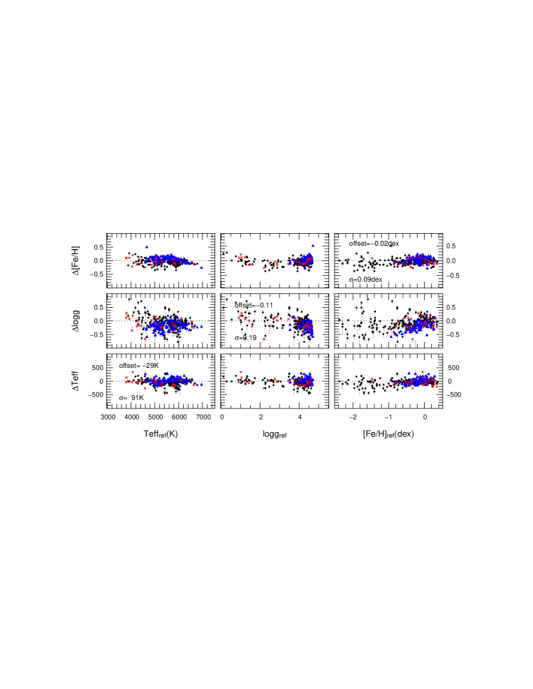
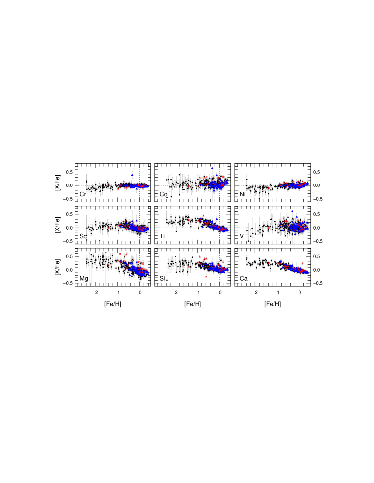
Despite the errors in stellar parameters, the resulting chemical abundances
are reliable, as shown in Fig. 18 and
Fig. 24 for synthetic and real spectra,
respectively. For the synthetic spectra the distribution of the derived chemical
abundances on the chemical plane follows closely the expected values (light colored
solid lines in Fig. 18), while for real
spectra the chemical abundance distributions follow fairly well the pattern
expected for the
Milky Way stars. A one-to-one comparison of the derived chemical abundances
with the reference abundances of the S4N spectra (Fig. 25)
reveals that some of the elements may suffer from systematic errors. In
particular Sc and Ti seem to be underestimated by 0.1 dex with
respect to the S4N estimations. For the
other elements, the abundances agree fairy well.
It is not clear what may cause the underestimation of the Sc and Ti .
The absorption lines of these two elements
are weak in the Sun, which makes the calibration
of the s and the determination of the abundances of the other
standard stars used for the calibration (Sec. 4)
difficult.
This can lead to a systematic offset of the calibrated s of the lines
of these elements, and therefore to an offset in the derived abundances.
On the other hand, in
Sec. 4.5 we showed how the calibrated s seems
to be smaller than the good quality s we took as reference. This would
lead to an overestimation of the chemical abundances, which is the opposite
of the underestimation seen. Moreover, it would affect all the elements and
not Sc and Ti alone.
Most of the systematic errors seen in synthetic spectra become
indistinguishable in the tests with real spectra, where the stochastic errors are larger.
However, there is at least one systematic error highlighted by the
tests on real spectra that must be discussed. It affects the and it is
discussed in the next section.
8.5.1 On the systematic error in in real spectra
The results obtained with synthetic and real spectra prove to be reliable and in fair agreement for all the stellar parameters but for , for which SP_Ace derives a too low gravity for metal poor spectra. The absence of this systematic error in the tests on synthetic spectra excludes that the error may originate in the way in which SP_Ace constructs the spectrum models. In the attempt to shed light on this, we tested SP_Ace with different settings, and we found that running SP_Ace with and without the keyword ABD_loop (which executes or skips the step 10 of the algorithm outlined in Sec.7) leads to results that are in agreement for all the stellar parameters but for . In Fig. 27 the residuals in are shown as a function of [Fe/H] for both settings for comparison purposes. With ABD_loop, real spectra show the systematic error just cited, whereas this is absent in synthetic spectra. Conversely, without ABD_loop the systematic error in for real spectra is greatly reduced, but the same systematic with opposite sign appears in synthetic spectra for the -enhanced stars (red crosses in Fig. 27) and not for the non-enhanced ones (green triangles). This seems to be in agreement with the real spectra, because for the stars here considered, the low metallicity stars are -enhanced too. This suggests that the only stars affected by this systematic are the -enhanced stars.

This indicates that the discrepancy observed between synthetic and real
spectra does not depend on the method employed, but that it may originate from
i) incorrect microturbulence adopted for the EW library or from
ii) the adopted 1D atmosphere models and LTE assumption, for which the discrepancy
to the physical conditions of real stars becomes larger for lower metallicity (Asplund
asplund2005, 2005; bergemann2012, 2012, Bergemann et al.). We are inclined to exclude that
the atomic parameters like damping constants or oscillator strengths may
play a significant role in this systematic error because otherwise it should equally
affect metal-rich and metal-poor stars.
The future development of a new GCOG library that accounts for NLTE effects and 3D
atmosphere models should shed light on the origin of this systematic and, hopefully,
remove it. Because this problem cannot be solved in the present work, we
choose to leave the option to the user whether to use the ABD_loop
keyword. In the appendix of this work, the
results of the tests on real spectra run without the ABD_loop
keyword are presented.
A further systematic error is the underestimation () of for dwarf ()stars. This effect is smaller in the
test with synthetic spectra than in real spectra.
The fact that for synthetic spectra this is small seems to
suggest that the origin of the problem may, as before, lie in the basic assumption made,
such as the LTE assumption and the stellar atmosphere models adopted.
8.6 Remark
In this paper we mostly aimed at validating the method proposed. For the sake of brevity, we do not discuss the tests done by using other functions available in SP_Ace and we just briefly mention two of them here202020The full list of functions available is provided with the tutorial that accompany the code SP_Ace.. SP_Ace accepts keywords like T_force and G_force that force SP_Ace to look for solutions with fixed and/or given by the user. This is particularly useful for low S/N spectra for which SP_Ace cannot converge to precise stellar parameters. For instance, a robust photometric temperature passed to SP_Ace with the keyword T_force helps to improve the and chemical abundances estimations. Another useful keyword is alpha which forces SP_Ace to derive the abundance of the -elements (Mg , Si , Ca and Ti ) as if they were one single element while any other elements (excluding C , N , and O ) are considered to be a separate single element called “metals”. As before, this is useful to get abundances from low-quality spectra that carry little information.
9 Publication
The source code of SP_Ace will be publicly available soon together with the line list and the GCOG library. The code will be released under a GPL license. In addition, a VO-integrated service allowing operation of SP_Ace without installation is available (Boeche et al. boeche2015, 2015). As simple Web front end to this service can be found at http://dc.g-vo.org/SP_ACE.
10 Future work
In this work we outlined the method the code SP_Ace relies upon and the solutions chosen up to now, which prove to work but are far from perfect. Many improvements and further developments are possible. Among the most important we cite the following ones:
-
•
Extension of the stellar parameter grid: it is possible to extend the coverage of the GCOG library to hotter temperature than the actual covered ones (7400 K) and to higher gravities. The latter have been extended to =5.4 with an extrapolation because stellar atmosphere models with 5.0 are not provided by the grid ATLAS9. An extension of the stellar atmosphere grid (and subsequent extension of the GCOG library) up to 6 is planned for the near future.
-
•
Extension of the line list: currently the wavelength range covered by the GCOG library is 5212-6860Å and 8400-8920Å. We plan to extend the wavelength range, in particular toward bluer wavelengths. With the extension of the grid to hotter stars, the line list will be augmented by ionized/high excitation potential lines only visible at high temperatures.
-
•
Molecular lines: at the present time the molecular lines we take in account are the CN lines in the range 8400-8920Å. An extension to the optical region would improve the derivation of stellar parameters for cool stars. How this problem can be solved in the framework of the method used by SP_Ace is still unclear.
-
•
Opacity correction: an improved method to correct the EW for the opacity of the neighboring lines has to be found. A further investigation of the rigorous solution proposed in Appendix B, or new techniques of line deconvolution (like the one proposed by Sennhauser et al. sennhauser, 2009) may lead to a solution.
-
•
Improved line profile: the present line profile adopted in SP_Ace is an empirical function that represents fairly well the shape of the lines over a wide range of parameters, but still is not good enough at the borders of the parameter grid. It is possible and desirable to find a new improved line profile function that would permit the removal of some of the systematic errors seen in synthetic spectra.
-
•
Extension to other stellar atmosphere models: the present EW library has been constructed with the 2012 version of the ATLAS9 atmosphere grid by Castelli & Kurucz castelli (2003), but it can be done with any other atmosphere models. The creation of EW and GCOG libraries based on MARCS (Gustafsson et al. gustafsson, 2008) or PHOENIX (Husser et al. husser, 2013) models is desirable and we plan to do it in the near future.
-
•
Extension to 3D models and NLTE assumptions: although the construction of a whole EW library with 3D atmosphere model and NLTE assumptions seems still prohibitive in terms of computing costs, the integration of the present EW library with few important absorption lines the EWs of which have been computed under NLTE assumptions and/or a 3D atmosphere model is doable. For instance, computing the EWs of H, the Fe I at 5269.537Å, and one line of the Ca II triplet with 3D atmosphere models and/or under NLTE assumptions and integrating these EWs into the present EW library would greatly increase the ability of SP_Ace to constrain the stellar parameters, in particular for low metallicity or low S/N spectra where only strong lines can be seen.
While for some of the above points the amount of work may be considerable, for other points the necessary work is small and it would bring significant improvements in a short time.

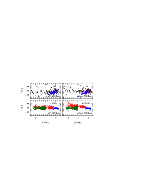
11 Conclusions
In this work we proposed and described a new method to derive stellar
parameters and chemical elemental abundances from stellar spectra. Based on calibrated
oscillator strengths of a complete line list and on 1D
atmosphere models and under LTE assumptions, this method relies on
polynomial functions (stored in the GCOG library) that describe the
EWs of the lines as a function of
the stellar parameters and chemical abundance. The method is implemented
in the code SP_Ace, which constructs on the fly spectral models and
minimizes the computed between the models and the observed spectrum.
The method has a full-spectrum-fitting approach, which means i) it assures the reliability
of the spectrum models by calibrating the oscillator strengths of the line
list adopted in high-resolution spectra of stars with well-known stellar
parameters, and ii) it employs all the possible absorption lines (thousands)
in a wide wavelength range to derive the stellar parameters and abundances,
exploiting the information carried by lines that are usually rejected in the classical
analysis because they are blended or have unreliable theoretical atomic parameters. This
approach proved to be successful, obtaining reliable stellar parameters and
chemical abundances even in spectra carrying little information,
such as low-resolution or low S/N spectra, for which the classical analysis
based on EW measurements cannot be applied.
The method is far from perfect, but we believe it shows considerable
promise already
at the present stage of development. It is highly automated, so
that it is suitable for the analysis of large spectroscopic surveys. It is
flexible, in the sense that its internal re-normalization and internal
re-setting of the radial velocity of the spectrum make SP_Ace independent
from the initial quality of the normalization and RV correction performed by
previous users or reduction pipelines. It is independent from the
stellar atmosphere models used to create the GCOG library on which
SP_Ace relies. In fact, the GCOG library can be constructed by using
any stellar atmosphere models available in the literature, or under LTE or NLTE
assumptions, with no need to change the code SP_Ace.
An on-line version of the code SP_Ace is available on the German Astrophysical Virtual Observatory web server at the address http://dc.g-vo.org/SP_ACE. The source code will be made publicly available soon.
Acknowledgements.
B.C. thanks: H.-G. Ludwig for the numerous useful discussions on atomic parameters and stellar atmosphere models; M. Demleitner and H. Heinl for their support in preparing the web front-end of SP_Ace and useful discussions. We acknowledge advice and assistance in publishing the web service provided by the German Astrophysical Virtual Observatory (GAVO). We acknowledge funding from Sonderforschungsbereich SFB 881 “The Milky Way System” (subproject A5) of the German Research Foundation (DFG).Appendix A Microturbulence
Because SP_Ace cannot determine the microturbulence, the EW library must be constructed by assuming the microturbulence value at each point of the grid before the EW computation. As done in a previous work (Boeche et al., boeche11, 2011) we can set the microturbulence as a function of the stellar parameters (see the work done by M. Bergemann and V. Hill in the Gaia-ESO collaboration cited in Jofré et al. jofre, 2014; Allende Prieto at al. allende, 2004). To determine such a function, we investigated how the microturbulence varies on the (, ) plane for some hundreds of stars studied in high-resolution spectroscopy works found in the literature (Fuhrmann fuhrmann, 1998; Allende Prieto et al. allende, 2004; Bensby et al. bensby, 2005; Fulbright et al. fulbright, 2006; Luck et al. 2006a, , 2006b, ; Luck & Heiter luck3, 2007; Luck et al. luck4, 2008). From such studies we used 620 derived microturbulence values for dwarfs, giants, and Cepheid stars to determine a polynomial function that approximates the microturbulence on the (, ) plane212121The total number of stars considered in these studies altogether is 921. Because the particularly high of some stars (mostly Cepheids) the fitting polynomial function was not satisfactory for normal stars. Because SP_Ace is designed manly for normal stars, we excluded stars with km s-1.. Such stars are shown in the left panel of Fig. 28. To fit we used a fourth-degree polynomial function. Higher degrees do not improve the fit. The polynomial function is written as follows:
| (7) |
where the coefficients are
| (8) | |||||
Because this polynomial function diverges to large positive values for high and low and to negative values at low and high , we imposed the following conditions: km s-1where km s-1and km s-1where km s-1. The values of the polynomial function and the just cited conditions on the (, ) plane are shown in the right panel of Fig. 28. In Fig. 29 the residuals between the computed and the literature works are shown together with the literature values as a function of . This polynomial function has been employed to set the microturbulence during the construction of the EW library.
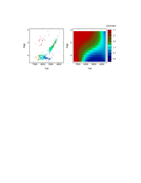
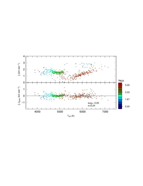
Appendix B Separating the contributions of different absorption lines to the total absorbed flux
In Sec. 5.2 we shortly discussed how to separate the contribution of blended lines to the total . Here we give a detailed explanation on how this can be done in the case of two blended lines. The extension to many lines is straightforward. Consider two blended absorption lines and the equation
| (9) |
where and are the individual contributions to the EW of
the blends of each absorption line and . We want to verify that
equation (9) is satisfied, or, in other words, that
and can be inferred from the radiative transfer
equation.
Because the EW of a line
is the measure of the absorbed flux over the line with respect
to the continuum, the previous problem is solved by verifying that
the flux (intensity of radiation ) emerging from a layer of a
stellar atmosphere over a small wavelength interval can be written as
| (10) |
where and are the individual absorbed intensities
due to the absorbers and , respectively. We are going to prove that
equation (10) is true for a layer that is homogeneous
in its physical conditions and chemical composition222222This can be
approximated by taking a very thin layer of a stellar atmosphere. The
1D atmosphere models are composed of layers that satisfy these
conditions.. Then we reach the answer by extending the result to the
whole atmosphere.
B.1 Pure absorption case
Consider one optically thick layer with two species of absorbers and
in it, and the variation of the radiation that goes through it.
The optical depth of the layer is . In the case of pure
absorption the transfer equation is
and the solution of this equation is
| (11) |
where is the intensity of the entering radiation,
is the intensity of the emerging radiation. We rearrange
equation (10) and using equation (11)
we write the absorbed intensity
| (12) |
We can ideally divide this optically thick layer (with optical deph ) in many optically thin layers, each of them with optical depth . Thus, for the -th thin layer we can write the equation (12) as follows:
where is the incoming intensity in the -th layer and
and are the optical depths of the -th layer due
to the and absorbers. By adopting the Taylor expansion of the exponential
function valid for optically thin layers, and
truncating it to the first order (the residual goes to zero when ), it
becomes
By writing
and
we separate the contributions of the absorbers and
to the absorbed intensities
| (13) |
Now we consider the ratio between the absorbed intensities
| (14) |
From equation (14) we isolate the term and
put it in equation (13) to obtain
| (15) |
We can write the contributions of the two absorbers and
as follows:
| (16) | |||||
| (17) |
where
Since the thick layer is homogeneous, what holds for the -th thin layer
(i.e., equations (16) and (17)), must hold for the whole
thick layer.
(This can actually be proved by using the limit .
The residual of the Taylor expansion goes to zero faster that , and
the equations (16) and (17) are therefore valid.)
Therefore, for the whole thick layer we can write
| (18) |
Because and are constant through the whole thick layer
( and do not change with ), we can write
| (19) | |||||
The terms
are the individual contributions to the
absorbed flux of the absorbers and , respectively.
By using equation (12),
and can be written as
and equation (10) is validated.
B.2 Atmosphere model case
Here we want to apply the previous result to an atmosphere model, which is
composed of number of layers (for instance, the Castelli & Kurucz atmosphere models
have ). Such
layers have different physical conditions, but inside every layer, the
physical conditions and the composition of the gas are
constants and homogeneous. Under such conditions,
the equations (B.1) are valid for every -th layer.
Consider the transfer equation
where and refer to two different absorbers and is the source function. The equation can also be written as
where , and
. grows from the bottom toward the
surface of the atmosphere, so that the optical depth is 0 at the bottom and
at the surface. is the monochromatic
intensity of the radiation in a plane-parallel atmosphere. The solution of this
equation is:
| (21) |
which gives the intensity of the flux at the optical depth . We can follow the intensity as function of the optical depth by subdividing the atmosphere into N layers, precisely at optical depths ,,…, and write
| (22) |
where and are the optical depths at the bottom and the top
of the -th layer, respectively, and is the incoming intensity at
the bottom of the -th layer (and the emerging intensity from the
-th layer). Because every layer has constant physical conditions
and constant optical thickness,
we can set the optical depths to match the optical depths
of the top of the -th layer of the atmosphere model. Because the constancy of the
physical conditions in each layer, the function of the integrand in
equation (22) is constant, and by solving the integral the equation
becomes:
| (23) |
where is the optical thickness of the -th layer,
is the source function and the incoming intensity in the -th
layer. Equation 23 is a
recurrence relation. The line of reasoning followed for
the case of pure absorption can be applied
to the source function as well. In fact, the product
is equivalent to the absorbed flux expressed in
equation (12).
Then, equations (10) and (18) can be applied to the two terms of
the sum in equation (23), and it becomes
| (24) |
where
| (25) | |||||
| (26) | |||||
| (27) | |||||
| (28) | |||||
| (29) | |||||
| (30) |
Rearranging the terms, equation (24) can be written as
where the values in the last two terms represent the contributed intensities of the lines A and B to the intensity after the -th layer.
B.3 Application to two blended lines
We applied the formula to the two lines OI at 8446.359Å (indicated with the letter ) and FeI at 8446.388Å (indicated with letter ) and solar atmosphere model. We also need to take in account the continuum absorption as third absorber. The continuum is indicated with the letter . For the -th layer the source function is
where and are the optical depth and opacity at the reference optical depth, and opacities of the continuum and the lines, is the Planck function, and the angle of view of the stellar disc, from the center () to the limb (). To follow how the radiation gets absorbed by the upper layers, we introduce a running index which runs from to and indicates the layers crossed by the radiation along its path to the surface. We start from the layer . The flux generated in the -th layer gets extincted in the same layer. The corresponding outcoming flux is then
where is the emerging radiation from the -th layer that was generated in the -th layer (in this case the layer is the same, ), and and are the optical depths of the -th layer due to the continuum and the two lines, respectively. The following layer absorbs the flux emerging from the -th layer, and the emerging flux from the -th layer is
| (32) |
and so on for the following layers. This is a recurrence formula, which continues until the layer (that is at the surface) is reached. For this surface layer the emerging radiation is
It represents the contribution function of the -th layer. At every -th layer we can compute the fraction of the radiation absorbed by the lines and by using the equations (27), (28), (29), and (30). Similarly, this can be done for the continuum . The quantity in equations (27) and (28) indicates the variation of intensity before and after the -th layer. This can be easily computed from the equation (32) by computing . Thus, the fractions of intensity absorbed by the two lines , , and the continuum in the -th layer are
| (33) | |||||
| (34) | |||||
| (35) |
By summing over the index in the equations (33), (34), and (35) we obtain the flux absorbed by the lines , , and . The contribution function of the -th layer can be therefore written as
| (36) |
where
By summing over the index in equation (36) we
obtain the total flux at angle .
To obtain the observed flux we must integrate from to .
The quantities of
the absorbed flux by the lines , , and the continuum are
illustrated in Fig. 30, where the logarithm of the
normalized flux is shown. The gray, red, and light blue areas show the flux absorbed by
the continuum, the OI line, and the FeI line, respectively.
This figure shows that by using the outlined way to
compute the flux we can estimate how much flux has been individually
absorbed by the lines in a blend. It is now clear why this
solution is not helpful in constructing the EW library we need:
while the classical EW refers to the flux
absorbed by a line with respect to the level of the continuum measured in
absence of the line, the absorbed flux obtained in
equation (36) is absolute and is much larger than the
EW because the continuum level and the emitted intensity change across the line.
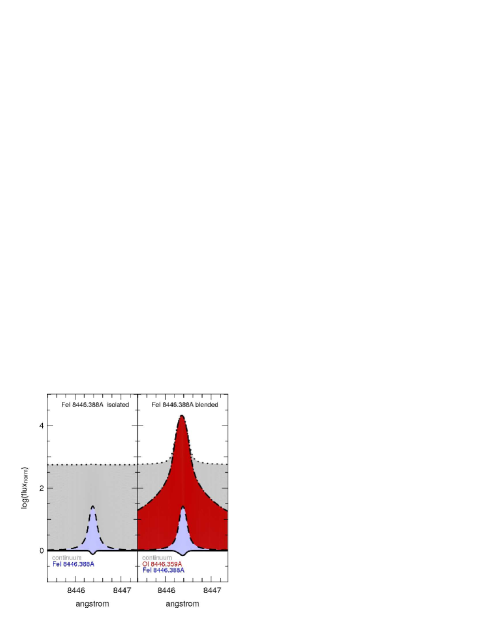
Appendix C The SP_Ace line profile
The shape of an absorption line is a function of many
variables (such as stellar parameters, atomic
parameters, chemical abundances, radial velocity of the atmosphere layers in
which the line forms) which cannot be analytically expressed
but only numerically computed through spectral synthesis.
However, experience says that spectral lines can be fairly
well described by a Voigt function, which
is the convolution of a Lorentzian function with a Gaussian function.
The Lorentzian FWHM () rules the width of the wings, while the
Gaussian FWHM () rules the width of the core of the Voigt
function.
Lines with larger damping constants have broader wings than the ones with
smaller damping constants, and the wings’ widths also vary with the gravity
of the star. Besides, the wings of the line
profile become broader (i.e., the ratios become bigger)
for larger EW232323For growing EW the core of the line grows slower
than the wings, therefore the line become broader..
Thus, the profile of an absorption line can be approximated with
a Voigt function in which and depend on the instrumental
FWHM, EW, and .
To allow SP_Ace to handle the shape of the absorption
lines, we adopted the Voigt function implementation given in
McLean et al. mclean (1994), modified to have
the equal to the instrumental FWHM, while follows the
empirical law
where EW is the equivalent width of the line, is the
“broadening” parameter (with ), and and are functions
of as described as follows
The parameter has been empirically derived by hand for each line
with a simple manual ”trial-and-error” method242424Out of
thousands of lines of the SP_Ace line list, the lines that
need are of the order of one hundred.
All the other lines have .
This allows us to find the parameter manually.:
the parameter is varied until the matches
between the line profile in the spectra models constructed by
SP_Ace and the line profile in five synthetic spectra of
different stellar parameters was satisfactory.
This empirical implementation of the line profile is satisfactory in most of
the stellar parameters here considered. However, progressive deviation from
the correct line profile is observed at K,
which causes systematic errors
(this is shown in tests with synthetic and real spectra in
Sec. 8).
The mismatch between the SP_Ace and the synthetic/real line profiles can be
reduced with a new improved line profile law that will be implemented in one
of the future releases of SP_Ace.
We here want to shortly discuss how the adopted line profile affects the performance of SP_Ace as a function of the spectral resolution. At low resolution the observed line profile is dominated by the instrumental profile, which is symmetric and constant for all the absorption lines. This characteristic makes the observed line profile easy to model. The higher the resolution, the more the physical profile of the lines dominates over the instrumental profile, making the observed profile difficult to model because, depending on the absorption line considered, the line can be asymmetric or deviate from the adopted Voigt function. Therefore, the line profile adopted by us matches at best the observed line profile at low resolution (where the instrumental profile dominates) and progressively loses accuracy at higher resolution. We verified that the accuracy of SP_Ace in reproducing the observed line profile is satisfactory up to R20 000. For higher resolutions the SP_Ace line profile may still be satisfactory for most of the absorption lines, but the robustness of the results has not been proved with extensive tests yet.
Appendix D Tests on real spectra
We report here the tables and the figures of the stellar parameters and chemical abundances derived with SP_Ace of the stellar spectra ELODIE, benchmark, and S4N degraded to R=12 000 and S/N=100.
| star | inf | sup | inf | sup | [M/H] | [M/H]inf | [M/H]sup | [Fe/H] | [Fe/H]inf | [Fe/H]sup | [Mg/H] | [Mg/H]inf | [Mg/H]sup | … | ||
|---|---|---|---|---|---|---|---|---|---|---|---|---|---|---|---|---|
| HD000245 | 5842 | 5663 | 5850 | 4.16 | 3.95 | 4.19 | -0.55 | -0.60 | -0.54 | -0.59 | -0.63 | -0.58 | -0.37 | -0.43 | -0.31 | … |
| HD000358 | 6182 | 6123 | 6215 | 4.03 | 3.97 | 4.11 | -0.30 | -0.33 | -0.28 | -0.29 | -0.31 | -0.28 | -0.32 | -0.39 | -0.26 | … |
| star | inf | sup | inf | sup | [M/H] | [M/H]inf | [M/H]sup | [Fe/H] | [Fe/H]inf | [Fe/H]sup | [Mg/H] | [Mg/H]inf | [Mg/H]sup | … | ||
|---|---|---|---|---|---|---|---|---|---|---|---|---|---|---|---|---|
| HD 49933 | 6570 | 6434 | 6582 | 4.03 | 3.87 | 4.10 | -0.49 | -0.53 | -0.48 | -0.50 | -0.53 | -0.49 | -0.42 | -0.51 | -0.36 | … |
| Hya | 5063 | 5014 | 5072 | 3.05 | 3.01 | 3.11 | 0.09 | 0.04 | 0.10 | 0.09 | 0.08 | 0.11 | 0.12 | 0.04 | 0.18 | … |
| star | inf | sup | inf | sup | [M/H] | [M/H]inf | [M/H]sup | [Fe/H] | [Fe/H]inf | [Fe/H]sup | [Mg/H] | [Mg/H]inf | [Mg/H]sup | … | ||
|---|---|---|---|---|---|---|---|---|---|---|---|---|---|---|---|---|
| Sun | 5685 | 5649 | 5705 | 4.28 | 4.25 | 4.31 | 0.04 | 0.02 | 0.05 | 0.04 | 0.03 | 0.06 | -0.04 | -0.8 | 0.00 | … |
| HIP 171 | 5330 | 5246 | 5354 | 4.08 | 3.96 | 4.09 | -0.82 | -0.88 | -0.80 | -0.82 | -0.85 | -0.80 | -0.51 | -0.56 | -0.43 | … |
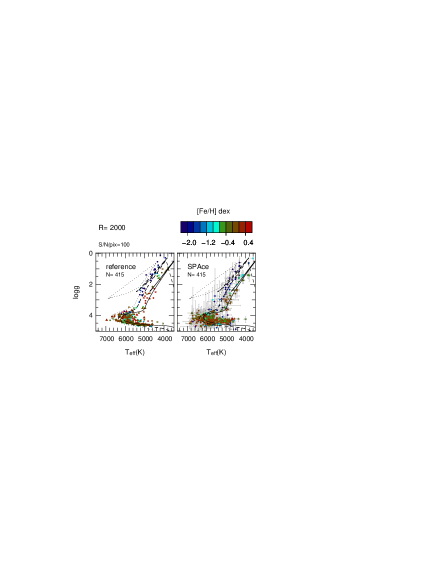
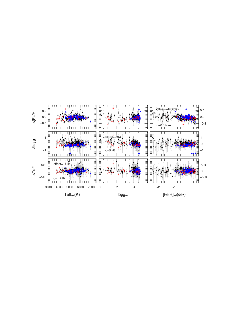
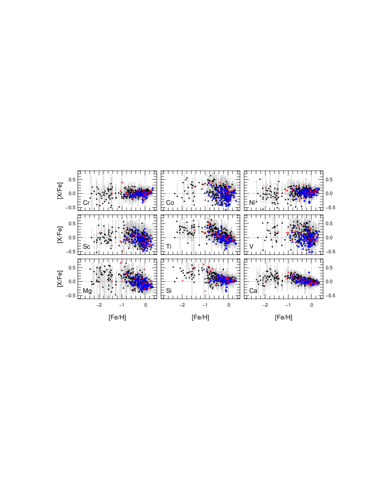
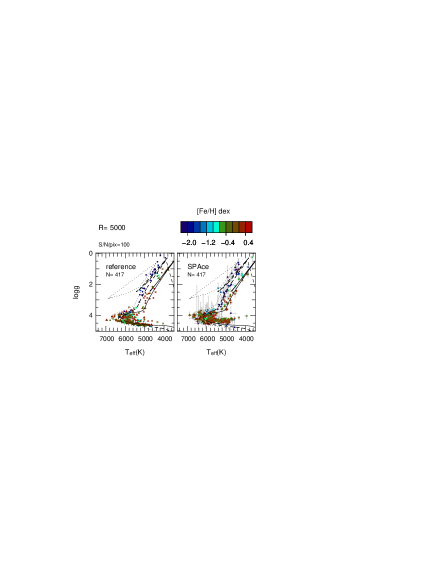
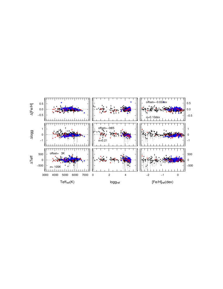
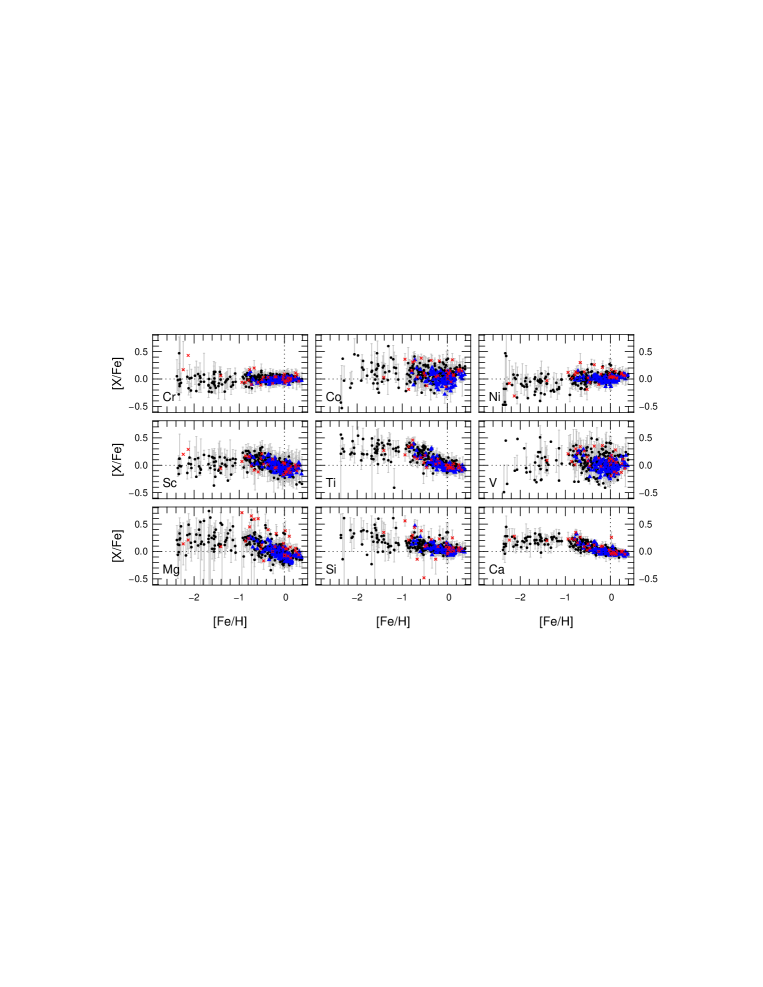
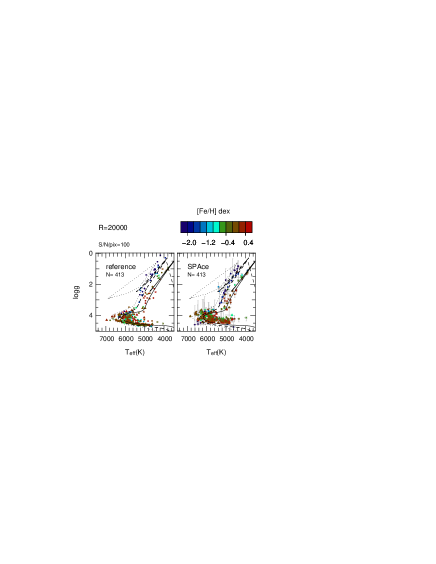
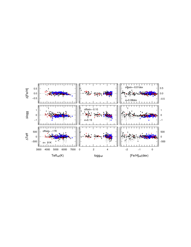
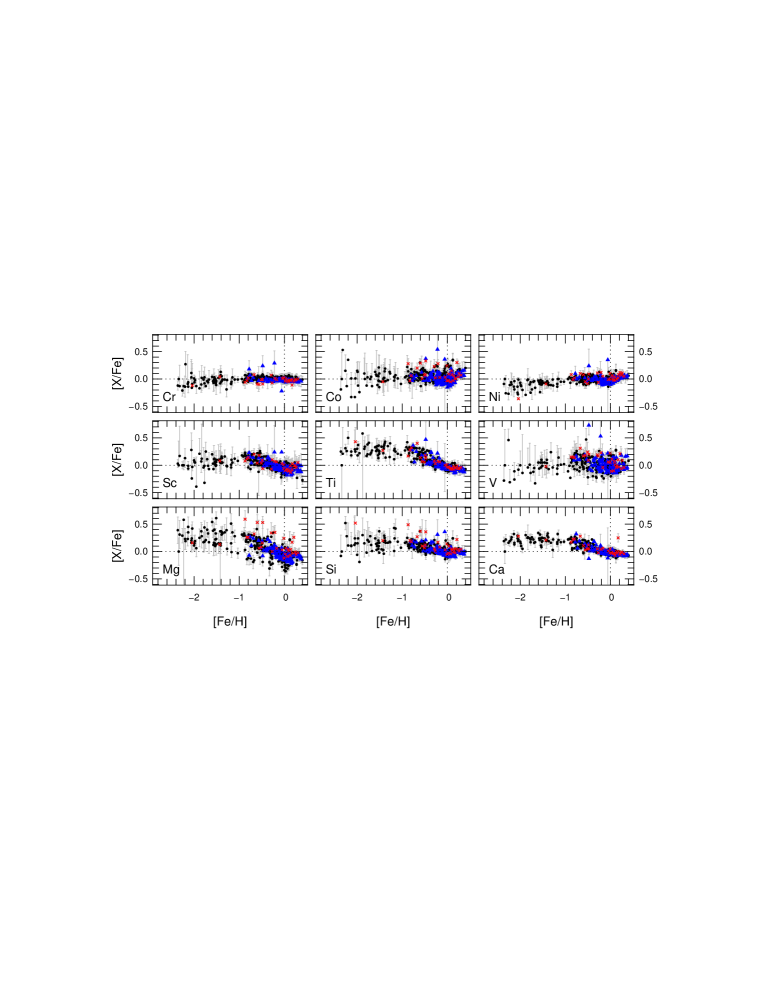
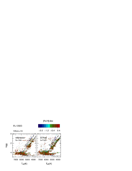
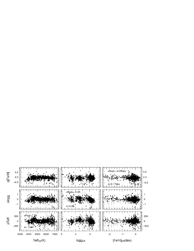
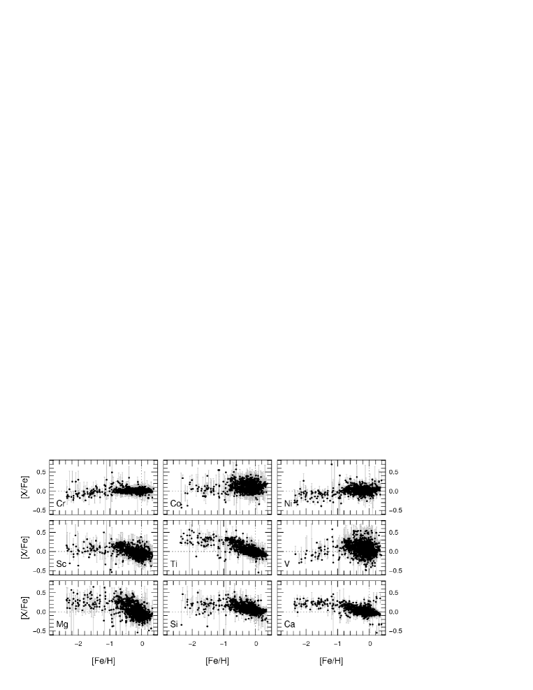
References
- (1) Allende Prieto, C., Barklem, P. S., Lambert, D. L., & Cunha, K. 2004, A&A, 420, 183
- (2) Allende Prieto, C., Beers, T. C., Wilhelm, R., et al. 2006, ApJ, 636, 804
- (3) Allende Prieto, C., Majewski, S. R., Schiavon, R., et al. 2008, Astronomische Nachrichten, 329, 1018
- (4) Asplund, M. 2005, ARA&A, 43, 481
- (5) Bailer-Jones, C. A. L. 1996, Ph.D. Thesis. Cambridge University
- (6) Barklem, P. S., Piskunov, N., & O’Mara, B. J. 2000, A&AS, 142, 467
- (7) Barklem, P. S., & Aspelund-Johansson, J. 2005, A&A, 435, 373
- (8) Bensby, T., Feltzing, S., Lundström, I., & Ilyin, I. 2005, A&A, 433, 185
- (9) Bergemann, M., Lind, K., Collet, R., Magic, Z., & Asplund, M. 2012, MNRAS, 427, 27
- (10) Bigot, L., & Thévenin, F. 2006, MNRAS, 372, 609
- (11) Blanco-Cuaresma, S., Soubiran, C., Jofré, P., & Heiter, U. 2014, A&A, 566, A98
- (12) Boeche, C., Siebert, A., Williams, M., et al., 2011, AJ, 142, 193
- (13) Boeche, C., Demleitner, M., Heinl, H., 2015, SP_Ace spectral analysis tool, VO resource ivo://org.gavo.dc/sp_ace/q/c, http://dc.g-vo.org/browse/sp_ace/q
- (14) Borrero, J. M., Bellot Rubio, L. R., Barklem, P. S., & del Toro Iniesta, J. C. 2003, A&A, 404, 749
- (15) Blackwell, D. E., & Collins, B. S. 1972, MNRAS, 157, 255
- (16) Blackwell, D. E., Ibbetson, P. A., Petford, A. D., & Willis, R. B. 1976, MNRAS, 177, 219
- (17) Blackwell, D. E., Petford, A. D., & Shallis, M. J. 1979, MNRAS, 186, 657
- (18) Blackwell, D. E., Petford, A. D., & Simmons, G. J. 1982, MNRAS, 201, 595
- (19) Simmons, G. J., & Blackwell, D. E. 1982, A&A, 112, 209
- (20) Bressan, A., Marigo, P., Girardi, L., et al. 2012, MNRAS, 427, 127
- (21) Castelli, F., Kurucz, R. L., 2003, in IAUS symp. 210, Modelling of Stellar Atmospheres, ed. N. Piskunov, W.W. Wiess and D.F. Gray , Published on behalf of the IAU by the ASP, 20
- (22) Chen, Y. Q., Nissen, P. E., Zhao, G., Zhang, H. W., & Benoni, T. 2000, A&AS, 141, 491
- (23) Chen, Y., Bressan, A., Girardi, L., et al. 2015, MNRAS, 452, 1068
- (24) de Jong, R. S., Bellido-Tirado, O., Chiappini, C., et al. 2012, Proc. SPIE, 8446, 84460T
- (25) Elia Garcia Perez, A., Allende-Prieto, C., Cunha, K. M., et al. 2014, American Astronomical Society Meeting Abstracts #223, 223, #440.07
- (26) Edvardsson, B., Andersen, J., Gustafsson, B., et al. 1993, A&A, 275, 101
- (27) Freytag, B., Steffen, M., Ludwig, H.-G., et al. 2012, Journal of Computational Physics, 231, 919
- (28) Fuhrmann, K. 1998, A&A, 338, 161
- (29) Fulbright, J. P., McWilliam, A., & Rich, R. M. 2006, ApJ, 636, 821
- (30) Gilmore, G., Randich, S., Asplund, M., et al. 2012, The Messenger, 147, 25
- (31) Grevesse, N., Sauval, A.J. 1998, Space Sci. Rev. 85, 161
- (32) Gurtovenko, E. A., & Kostik, R. I. 1981, A&AS, 46, 239
- (33) Gurtovenko, E. A., & Kostik, R. I. 1982, A&AS, 47, 193
- (34) Gustafsson, B., Edvardsson, B., Eriksson, K., et al. 2008, A&A, 486, 951
- (35) Hinkle, K. H., & Lambert, D. L. 1975, MNRAS, 170, 447
- (36) Hinkle, K., Wallace, L., Harmer, D., Ayres, T., & Valenti, J. 2000, IAU Joint Discussion, 1 Visible and Near Infrared Atlas of the Arcturus Spectrum 3727-9300 , Available at: ftp://ftp.noao.edu/catalogs/arcturusatlas/visual
- (37) Holweger, H. 1971, A&A, 10, 128
- (38) Holweger, H. 1973, A&A, 26, 275
- (39) Holweger, H., & Mueller, E. A. 1974, Sol. Phys., 39, 19
- (40) Holweger, H., Heise, C., & Kock, M. 1990, A&A, 232, 510
- (41) Husser, T.-O., Wende-von Berg, S., Dreizler, S., et al. 2013, A&A, 553, A6
- (42) Ivanauskas, A., Kucinskas, A., Ludwig, H. G., & Caffau, E. 2010, Nuclei in the Cosmos, 290
- (43) Jofré, P., Heiter, U., Soubiran, C., et al. 2014, A&A, 564, A133
- (44) Jofré, P., Heiter, U., Soubiran, C., et al. 2015, A&A, 582, A81
- (45) Koleva, M., Prugniel, P., Bouchard, A., & Wu, Y. 2009, A&A, 501, 1269
- (46) Kramida, A., Ralchenko, Yu., Reader, J., and NIST ASD Team (2013). NIST Atomic Spectra Database (ver. 5.1). Available: http://physics.nist.gov/asd. National Institute of Standards and Technology, Gaithersburg, MD.
- (47) Kirby, E. N., Guhathakurta, P., & Sneden, C. 2008, ApJ, 682, 1217
- (48) Kordopatis, G., Gilmore, G., Steinmetz, M., et al. 2013, AJ, 146, 134
- (49) Kupka, F., Piskunov, N., Ryabchikova, T. A., Stempels, H. C., & Weiss, W. W. 1999, A&AS, 138, 119
- (50) Kurucz, R. L., & Peytremann, E. 1975, SAO Special Report, 362, part 1
- (51) Kurucz, R. L. 1995, in ASP Conf.Ser 78, Astrophysical Application of Powerful New Database, ed. S.J. Adelman, W.L. Wiese, (San Francisco, CA), 205
- (52) Lindegren, L., Babusiaux, C., Bailer-Jones, C., et al. 2008, IAU Symposium, 248, 217
- (53) Lobel, A. 2011, Canadian Journal of Physics, 89, 395
- (54) Luck, R. E., & Heiter, U. 2006, AJ, 131, 3069
- (55) Luck, R. E., Kovtyukh, V. V., & Andrievsky, S. M. 2006, AJ, 132, 902
- (56) Luck, R. E., & Heiter, U. 2007, AJ, 133, 2464
- (57) Luck, R. E., Andrievsky, S. M., Fokin, A., & Kovtyukh, V. V. 2008, AJ, 136, 98
- (58) Maeckle, R., Holweger, H., Griffin, R., & Griffin, R. 1975, A&A, 38, 239
- (59) Magic, Z., Collet, R., Asplund, M., et al. 2013, A&A, 557, A26
- (60) Magrini, L., Randich, S., Friel, E., et al. 2013, A&A, 558, A38
- (61) Martins, L. P., Coelho, P., Caproni, A., & Vitoriano, R. 2014, MNRAS, 442, 1294
- (62) McLean A.B., Mitchell C.E.J., & Swanston D.M., 1994, J. Electron Spectrosc. Relat. Phenom., 69, 125
- (63) Mucciarelli, A., Pancino, E., Lovisi, L., Ferraro, F. R., & Lapenna, E. 2013, ApJ, 766, 78
- (64) Ness, M., Hogg, D. W., Rix, H.-W., Ho, A. Y. Q., & Zasowski, G. 2015, ApJ, 808, 16
- (65) Oneill, J. A., & Smith, G. 1980, A&A, 81, 100
- (66) Perryman, M. A. C., de Boer, K. S., Gilmore, G., et al. 2001, A&A 369, 339
- (67) Plez, B. 2008, Physica Scripta Volume T, 133, 014003
- (68) Posbic, H., Katz, D., Caffau, E., et al. 2012, A&A, 544, A154
- (69) Prugniel, P., Soubiran, C., Koleva, M., & Le Borgne, D. 2007, VizieR Online Data Catalog, 3251, 0
- (70) Press, W.H., Teukolsky, S.A., Vetterling, W.T., Flannery, B.P., 1992, Numerical Recipes: The Art of Scientific Computing (2nd ed.), New York: Cambridge University Press, ISBN 0-521-43064-X.
- (71) Ramírez, I., & Allende Prieto, C. 2011, ApJ, 743, 135
- (72) Recio-Blanco, A., Bijaoui, A., & de Laverny, P. 2006, MNRAS, 370, 141
- (73) Reddy, R. R., Nazeer Ahammed, Y., Rama Gopal, K., & Baba Basha, D. 2003, Ap&SS, 286, 419
- (74) Ruffoni, M. P., Allende Prieto, C., Nave, G., & Pickering, J. C. 2013, ApJ, 779, 17
- (75) Ruffoni, M. P., Den Hartog, E. A., Lawler, J. E., et al. 2014, MNRAS, 441, 3127
- (76) Sbordone, L., Caffau, E., Bonifacio, P., & Duffau, S. 2014, A&A, 564, A109
- (77) Schweitzer, A., Hauschildt, P. H., Baron, E., & Allard, F. 2003, Stellar Atmosphere Modeling, 288, 339
- (78) Seaton, M. J., Yan, Y., Mihalas, D., & Pradhan, A. K. 1994, MNRAS, 266, 805
- (79) Sennhauser, C., Berdyugina, S. V., & Fluri, D. M. 2009, A&A, 507, 1711
- (80) Smith, V. V., Cunha, K., Shetrone, M. D., et al. 2013, ApJ, 765, 16
- (81) Sneden, C., 1973, Ph.D. thesis, Univ. Texas ar Austin
- (82) Sousa, S. G., Santos, N. C., Israelian, G., Mayor, M., & Monteiro, M. J. P. F. G. 2007, A&A, 469, 783
- (83) Steinmetz, M., Zwitter, T., Siebert, A., et al. 2006, AJ, 132, 1645
- (84) Thévenin, F. 1989, A&AS, 77, 137
- (85) Thévenin, F. 1990, A&AS, 82, 179
- (86) Valenti, J. A., & Piskunov, N. 1996, A&AS, 118, 595
- (87) Wedemeyer, S. 2001, A&A, 373, 998
- (88) Yanny, B., Rockosi, C., Newberg, H. J., et al. 2009, AJ, 137, 4377
- (89) Zhao, G., Zhao, Y.-H., Chu, Y.-Q., Jing, Y.-P., & Deng, L.-C. 2012, Research in Astronomy and Astrophysics, 12, 723
- (90) Zucker, D. B., de Silva, G., Freeman, K., Bland-Hawthorn, J., & Hermes Team 2012, Galactic Archaeology: Near-Field Cosmology and the Formation of the Milky Way, 458, 421