Turbulent Magnetohydrodynamic Reconnection Mediated by the Plasmoid Instability

Abstract

It has been established that the Sweet-Parker current layer in high Lundquist number reconnection is unstable to the super-Alfvénic plasmoid instability. Past two-dimensional magnetohydrodynamic simulations have demonstrated that the plasmoid instability leads to a new regime where the Sweet-Parker current layer changes into a chain of plasmoids connected by secondary current sheets, and the averaged reconnection rate becomes nearly independent of the Lundquist number. In this work, three-dimensional simulation with a guide field shows that the additional degree of freedom allows plasmoid instabilities to grow at oblique angles, which interact and lead to self-generated turbulent reconnection. The averaged reconnection rate in the self-generated turbulent state is of the order of a hundredth of the characteristic Alfvén speed, which is similar to the two-dimensional result but is an order of magnitude lower than the fastest reconnection rate reported in recent studies of externally driven three-dimensional turbulent reconnection. Kinematic and magnetic energy fluctuations both form elongated eddies along the direction of local magnetic field, which is a signature of anisotropic magnetohydrodynamic turbulence. Both energy fluctuations satisfy power-law spectra in the inertial range, where the magnetic energy spectral index is in the range from $-2.3$ to $-2.1$, while the kinetic energy spectral index is slightly steeper, in the range from $-2.5$ to $-2.3$. The anisotropy of turbulence eddies is found to be nearly scale-independent, in contrast with the prediction of the Goldreich-Sridhar theory for anisotropic turbulence in a homogeneous plasma permeated by a uniform magnetic field.

1 Introduction

Magnetic reconnection is a process that changes the topology of magnetic field lines and releases magnetic energy in the form of plasma kinetic, thermal, or nonthermal energy. It is widely believed to be the underlying mechanism that powers explosive events such as geomagnetic substorms, solar flares, coronal mass ejections (CMEs), gamma-ray bursts, as well as sawtooth crashes in fusion plasmas (Biskamp, 2000; Priest & Forbes, 2000; Zweibel & Yamada, 2009; Yamada et al., 2010). Large-scale space and astrophysical environments where magnetic reconnection takes place, such as solar corona, solar wind, interstellar medium, molecular clouds, and accretion disks, are known to be turbulent (Rickett, 1990; Narayan, 1992; Balbus & Hawley, 1998; Lazarian et al., 2012b). Therefore, how turbulence and reconnection influence each other is a question of great importance. Broadly speaking, the interplay between turbulence and reconnection can be viewed from two complementary perspectives. On the one hand, there can be many small-scale reconnection events simultaneously taking place in a large-scale turbulent bath (Rappazzo et al., 2008; Servidio et al., 2009, 2010; Rappazzo et al., 2010; Servidio et al., 2011; Wan et al., 2014), which may provide an energy source to heat the plasma, e.g. as in the nanoflare scenario of coronal heating (Parker, 1988). On the other hand, small-scale turbulence may also affect the reconnection of a large-scale, coherent magnetic field (Lazarian & Vishniac, 1999; Kowal et al., 2009; Loureiro et al., 2009; Eyink et al., 2011; Lazarian et al., 2012a, 2015a, 2015b). This latter aspect may have significant implications in the energy release of large-scale eruptions, such as coronal mass ejections (CMEs), and is the main concern of this study.

Traditionally, theoretical studies of magnetic reconnection have been mostly focused on two-dimensional (2D) models (e.g. the classical Sweet-Parker (Sweet, 1958; Parker, 1957) and Petschek (Petschek, 1964) models) under the assumption that reconnection occurs in a single, stable current sheet. In recent years, there is growing evidence that large-scale reconnection is likely to take place in a fragmented reconnection layer, due to the presence of secondary instabilities, which are found in a wide range of plasma models, including resistive magnetohydrodynamics (MHD) (Biskamp, 1986; Shibata & Tanuma, 2001; Loureiro et al., 2007; Lapenta, 2008; Bhattacharjee et al., 2009; Cassak et al., 2009; Huang & Bhattacharjee, 2010; Bárta et al., 2011; Huang et al., 2011; Shen et al., 2011; Loureiro et al., 2012; Ni et al., 2012; Huang & Bhattacharjee, 2012, 2013; Takamoto, 2013; Wyper & Pontin, 2014), Hall MHD (Shepherd & Cassak, 2010; Huang et al., 2011), and fully kinetic particle-in-cell (PIC) simulations (Daughton et al., 2006, 2009, 2011; Fermo et al., 2012; Daughton et al., 2014). Among these secondary instabilities, the plasmoid (or secondary tearing) instability in resistive MHD (Loureiro et al., 2007; Bhattacharjee et al., 2009) has been extensively studied in recent years. Through high-resolution 2D simulations, it is now established that the plasmoid instability leads to fast reconnection in resistive MHD with the reconnection rate nearly independent of the resistivity (Bhattacharjee et al., 2009; Huang & Bhattacharjee, 2010; Loureiro et al., 2012). When three-dimensional (3D) perturbations are allowed in a reconnection configuration with a guide field, oblique tearing modes with resonant surfaces (i.e. where $\mathbf{k}\cdot\mathbf{B}=0$) away from the mid-plane can be excited in addition to the usual 2D modes (Baalrud et al., 2012). In this work, we examine the possibility of establishing self-sustained turbulent reconnection via the interaction between oblique tearing modes, in contrast to previous MHD studies where turbulence is driven through external forcing (Kowal et al., 2009; Loureiro et al., 2009). Realizing self-sustained turbulent reconnection is essential for further comparison with observations, as results from externally forced turbulent reconnection will inevitably depend on the input power. Although self-sustained turbulent reconnection through interacting oblique modes has been reported in a recent fully kinetic collisionless PIC simulation by Daughton et al. (2011), the simulation system size is limited to the order of several tens of ion skin depths, which is substantially too small from an astrophysical point of view. To give an example, typical values of ion skin depth in the solar corona are in the range of $1$ – $100$ meters, whereas the extent of a post-CME current sheet can be more than $10^{9}$ meters (Ciaravella & Raymond, 2008). From this perspective, our study complements that in Daughton et al. (2011) by focusing on large-scale dynamics where a MHD description is applicable, while neglecting kinetic physics that may be important at small scales. In addition, because theories of anisotropic turbulence are much more well developed for MHD than they are for collisionless plasmas, we are able to apply well established diagnostics and make quantitative comparisons with existing MHD turbulence theories.

This paper is organized as follows. Section 2 gives a detailed description of the simulation setup. The simulation results are presented in Section 3, which is divided into two parts. Section 3.1 gives an overall description of the time evolution and development of turbulence, and makes comparison with corresponding 2D simulations with and without plasmoids. Section 3.2 looks more deeply into the characteristics of the fully developed turbulent state, including power-law spectra of the inertial range, eddy anisotropy with respect to local magnetic field, and comparisons with the Goldreich-Sridhar theory of MHD turbulence (Goldreich & Sridhar, 1995, 1997). Finally, we discuss the implications of our findings for large-scale astrophysical reconnection and conclude in Section 4.

2 Simulation Setup

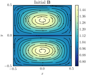
Figure 1: Initial magnetic field configuration. Black lines are stream lines of the in-plane component, and color shading shows the out-of-plane component $B_{z}$.

The governing equations of our numerical model are the standard nondimensionalized compressible, viscous, and resistive magnetohydrodynamics with an adiabatic equation of state:

$$\partial_{t}\rho+\nabla\cdot\left(\rho\mathbf{v}\right)=0,$$ (1)

$$\partial_{t}\left(\rho\mathbf{v}\right)+\nabla\cdot\left(\rho\mathbf{vv}\right)=-\nabla\left(p+\frac{B^{2}}{2}\right)+\nabla\cdot(\mathbf{BB})+\nu\nabla^{2}(\rho\mathbf{v}),$$ (2)

$$\partial_{t}p+\nabla\cdot(p\mathbf{v})=-(\gamma-1)p\nabla\cdot\mathbf{v},$$ (3)

$$\partial_{t}\boldsymbol{B}=\nabla\times\left(\mathbf{v}\times\boldsymbol{B}-\eta\mathbf{J}\right),$$ (4)

where standard notations are used. The electric current density $\mathbf{J}$ is related to the magnetic field $\mathbf{B}$ via the relation $\mathbf{J}=\nabla\times\mathbf{B}$. The numerical algorithm is detailed in (Guzdar et al., 1993). Derivatives are approximated by a five-point central finite difference scheme, with a fourth-order numerical dissipation equivalent to up-wind finite difference added to all equations for numerical stability. Time stepping is calculated by a trapezoidal leapfrog scheme. Explicit dissipations are employed through viscosity and resistivity.

We use a simulation setup that has been employed in previous studies (Huang & Bhattacharjee, 2010; Huang et al., 2011; Huang & Bhattacharjee, 2012), where the attraction between two coalescing magnetic flux tubes is the driver of magnetic reconnection. The simulation box is a 3D cube in the domain $(x,y,z)\in[-1/2,1/2]\times[-1/2,1/2]\times[-1/2,1/2]$. In normalized units, the initial magnetic field is given by $\mathbf{B}=B_{z}\mathbf{\hat{z}}+\mathbf{\hat{z}}\times\nabla\psi$, where $\psi=\tanh\left(y/h\right)\cos\left(\pi x\right)\sin\left(2\pi y\right)/2\pi$, and $B_{z}$ is non-uniform such that the initial configuration is approximately force-balanced (Figure 1). The parameter $h$, which is set to $1/300$ for this study, determines the initial width of the current layer between the flux tubes. In the upstream region of the current layer, the reconnecting component $B_{x}$ and the guide field $B_{z}$ are both approximately unity. The initial plasma density and temperature are both uniform, with $\rho=1$ and $T=1$ in normalized units. The viscosity $\mu$ and resistivity $\eta$ are both set to $5\times 10^{-6}$, which give a Lundquist number $S\equiv V_{A}L/\eta=2\times 10^{5}$ and a magnetic Prandtl number $Pr_{m}\equiv\mu/\eta=1$. The heat capacity ratio $\gamma=5/3$ is assumed. Perfectly conducting and free slipping boundary conditions are imposed along both $x$ and $y$ directions, and periodic boundary conditions along $z$. The simulation mesh size is $N_{x}\times N_{y}\times N_{z}=2000\times 1000\times 2000$, where the grid sizes are uniform along both $x$ and $z$ directions, and packed along the $y$ direction around the midplane to better resolve the reconnection layer. The grid size along $y$ near the midplane ($y=0$) is $\Delta y=10^{-4}$, which gradually increases away from the midplane and reaches $\Delta y=0.005$ near the boundary. The resolution on the $x-y$ plane is based on our extensive experience from a 2D scaling study (Huang & Bhattacharjee, 2010), where simulations with different resolutions have been performed. In this study, we have also performed the same simulation with $N_{z}=1000$ and $2000$ and found no significant difference. To trigger the plasmoid instability, the initial velocity is seeded with a random noise of amplitude $10^{-3}$. This is in contrast with the situation in particle-in-cell codes, where noise associated with a finite number of particles is enough to trigger the plasmoid instability.

3 Simulation Results

3.1 Time Evolution and Reconnection Rate

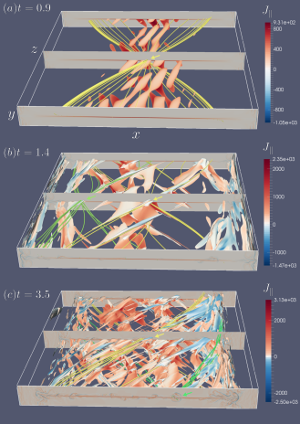
Figure 2: Snapshots of the 3D simulation at three representative times. Color shading shows the component of the electric current parallel to the magnetic field $J_{\parallel}\equiv\mathbf{J}\cdot\mathbf{\hat{b}}$ on three $x-y$ slices, as well as on isosurfaces of the fluctuating part of the magnetic energy $\tilde{E_{m}}=|\tilde{\mathbf{B}}|^{2}/2$. These snapshots also show samples of magnetic field lines, where field lines with the same color are originated from a selected small region as indicated by an arrow of the same color. These plots show the entire $x$ and $z$ dimensions of the simulation box, but only the region $-0.05\leq y\leq 0.05$ along the $y$ direction.

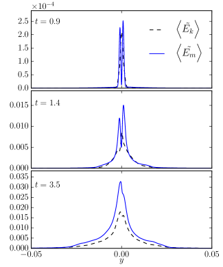
Figure 3: One-dimensional profiles (along $y$) of the averaged kinetic energy fluctuation $\left\langle\tilde{E_{k}}\right\rangle$ and magnetic energy fluctuation $\left\langle\tilde{E_{m}}\right\rangle$, corresponding to the three snapshots of Figure 2. Here the averaging is carried out over the central part of the reconnection layer within the range $-0.25\leq x\leq 0.25$ and the entire $z$ direction.

Our primary interest of this study is to understand how small-scale turbulence affects reconnection of a large-scale “mean” magnetic field. To separate the large-scale mean field from small-scale fluctuations, the former must be determined through an averaging procedure (or coarse-graining). Two commonly used definitions for the mean field are ensemble average and time average. The former is obtained via averaging over the ensemble of all turbulent realizations (e.g., from different initial random noise) of the same setting, whereas the latter is obtained by averaging over an appropriate period of time. If we further assume ergodicity (see, e.g. the discussion in Frisch (1995)), ensemble average and time average are nearly equivalent. In practice, a time average is often adopted, because an ensemble average requires, by definition, many different realizations of the same setup, which can be prohibitively expensive. However, because the system under consideration has a translational symmetry along the $z$ direction, i.e. $z$-dependence only arises as a result of instabilities, after averaging over the entire ensemble, the mean field must be independent of $z$. Therefore, instead of using a time average, we adopt the convention of using the average of a physical variable $f$ over the entire $z$ direction as the mean field $\bar{f}$, which is taken as a proxy for the ensemble average. Once the mean field is determined, the fluctuation is obtained by the remaining part $\tilde{f}\equiv f-\bar{f}$ . This procedure ensures that the mean magnetic field $\bar{\mathbf{B}}$ is independent of $z$, and consequently we may calculate the 3D reconnection rate in terms of $\bar{\mathbf{B}}$ in the same way as in 2D cases. We should note, however, that this procedure is not applicable for more general situations when the initial condition is dependent on all three coordinates. In that case, an appropriate definition for the mean field will be a time average over a period of time sufficiently longer than typical turbulence eddy turnover time, but shorter than evolution time scales of large scale field. The resulting mean field in general will depend on all three coordinates. Nevertheless, a general definition of reconnection rate in full 3D configurations remains a topic of debate, which is beyond the scope of this work. See, e.g. the discussion in (Huang et al., 2014; Daughton et al., 2014; Wyper & Hesse, 2015) and the references therein.

We begin by examining the time evolution and development of turbulence in the reconnection layer. Figure 2 shows three representative snapshots of the reconnection layer, where color shading shows the component of the electric current parallel to the magnetic field $J_{\parallel}\equiv\mathbf{J}\cdot\mathbf{\hat{b}}$ on three $x-y$ slices, as well as on isosurfaces of the fluctuating part of the magnetic energy $\tilde{E_{m}}=|\tilde{\mathbf{B}}|^{2}/2$. These snapshots also show samples of magnetic field lines, where field lines with the same color originate from a selected small region as indicated by an arrow of the same color. Here the isosurfaces in each snapshot correspond to a single value of $\tilde{E_{m}}$; they are employed as a means to visualize the development of complex structures as the instabilities evolve. The color shaded parallel electric current $J_{\parallel}\equiv\mathbf{J}\cdot\mathbf{\hat{b}}$ is employed as a proxy for showing where non-ideal effects are concentrated. Panel (a) shows an early phase when the plasmoid instabilities are developing, at $t=0.9$. It shows that magnetic fluctuations initially develop preferentially at oblique angles, at locations slightly away from the midplane. At this time the Sweet-Parker current sheet is still largely unperturbed. Panel (b) shows a snapshot at $t=1.4$, when the instabilities have further developed, and some coherent structures start to become visible on the $x-y$ slices of the $J_{\parallel}$ profiles. Panel (c) shows a snapshot at $t=3.5$, when the instabilities have developed into a fully turbulent state. At this time, the isosurfaces of $\tilde{E_{m}}$ form complicated structures, which appear to align preferentially with magnetic field lines. This is an important feature that we will come back to at later discussion. The $x-y$ slices of $J_{\parallel}$ also show blob-like structures which give the impression that they may be cross sections of magnetic flux ropes. However, tracing field lines from the blobs shows that not to be the case. The two sets of field lines (indicated by yellow and green colors, respectively) in panel (c) both originate from a blob-like structure, but the field lines clearly show the influence of the global magnetic shear across the reconnection layer. Each set of field lines roughly separates into two bundles, one approximately follows the magnetic field above the reconnection layer, while the other approximately follows the magnetic field below the layer. In these two sets of field lines, however, some neighboring field lines are found to wrap around each other over a certain distance, which may be loosely interpreted as indicative of flux ropes.

To see how the turbulent region broadens as the instabilities develop, we calculate the one-dimensional (1D) profiles of averaged kinetic energy fluctuation $\left\langle\tilde{E_{k}}\right\rangle$ and magnetic energy fluctuation $\left\langle\tilde{E_{m}}\right\rangle$ along the $y$ direction. Here the averaging is carried out over the central part of the reconnection layer within the range $-0.25\leq x\leq 0.25$ and the entire $z$ direction. Because we employ a compressible MHD model, the kinetic energy fluctuation is defined through a new variable $\mathbf{w}\equiv\sqrt{\rho}\mathbf{u}$ (Kida & Orszag, 1992) such that the kinetic energy density $E_{k}=w^{2}/2$ is a quadratic form of $w$ and the fluctuation part of kinetic energy density is defined as $\tilde{E_{k}}\equiv\left|\tilde{\mathbf{w}}\right|^{2}/2$. Figure 3 shows the resulting 1D profiles corresponding to the three snapshots of Figure 2. The top panel at $t=0.9$ shows that $\left\langle\tilde{E_{m}}\right\rangle$ has two peaks, corresponding to the regions of magnetic energy fluctuations growing at oblique angles in Figure 2 (a). In contrast, the kinetic energy fluctuation $\left\langle\tilde{E_{k}}\right\rangle$ peaks at the center around $y=0$. These energy fluctuations are localized to a narrow layer within the Sweet-Parker layer. As the instabilities develop, the energy fluctuations gradually spread out to a broader region, shown in the middle panel at $t=1.4$. At this time the magnetic energy fluctuation profile still exhibits two peaks. The bottom panel of Figure 3 shows the fully developed state at $t=3.5$, when the turbulent region becomes even broader. At this time the double-peak structure of $\left\langle\tilde{E_{m}}\right\rangle$ has almost disappeared. Magnetic fluctuations carry more energy than kinetic fluctuations, and approximately $70\%$ of the total energy fluctuation is contained in the range $-0.01\leq y\leq 0.01$.

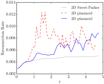
Figure 4: Time histories of reconnection rates for the three runs.

As mentioned in the Introduction, it has been established that the plasmoid instability leads to fast reconnection in 2D resistive MHD with the reconnection rate nearly independent of the resistivity. An important question is how 3D effects affect the overall reconnection rate. To facilitate a comparison, we carry out two additional 2D simulations with the same setting. The first one without initial random noise realizes Sweet-Parker reconnection, whereas the second one with an initial random noise of the same amplitude as the 3D case results in 2D plasmoid-dominated reconnection. We measure the reconnection rate in the following way. First we use the mean field $\bar{\mathbf{B}}$ (which is simply $\mathbf{B}$ in 2D cases) to calculate the reconnected magnetic flux as the maximum of the flux function $\psi(x)\equiv\int_{-1/2}^{x}\bar{B_{y}}(x^{\prime})dx^{\prime}$ along the midplane ($y=0$). Its time derivative $d\psi/dt$ then gives the instantaneous reconnection rate. Figure 4 shows the time histories of the reconnection rates for the three cases. The three curves coincide with each other at the beginning. The plasmoid instability sets in at an earlier time $t\simeq 0.5$ in the 2D simulation, and the reconnection rate rapidly increases and reaches the peak value $d\psi/dt\simeq 0.012$ at $t\simeq 1.5$, then decreases to a quasi-steady plateau that fluctuates around $d\psi/dt\simeq 0.008$. In contrast, the plasmoid instability in the 3D simulation sets in at a relatively later time $t\simeq 0.9$. The reconnection rate does not rapidly increase to a peak then decreases as in the 2D case. Instead, it gradually increases and reaches a quasi-steady value that is comparable to the 2D counterpart and appears to be slightly increasing over time. Not surprisingly, the Sweet-Parker run gives the slowest reconnection rate, which approximately reaches $d\psi/dt\simeq 0.004$ after the initial current sheet thinning period, and slightly increases over the entire simulation time and reaches $d\psi/dt\simeq 0.005$ at the end of the simulation. The slowly increasing reconnection rates in both Sweet-Parker reconnection and 3D turbulent reconnection may be attributed to gradual evolution of the global configuration. This simulation setup does not allow a true steady state as the two merging flux tubes that drive the reconnection process shrink in size as time passes. The reconnection rates of the 2D and 3D simulations with plasmoid instabilities are less than a factor of two higher than the Sweet-Parker reconnection rate. This relatively low enhancement of reconnection rate is due to the modest value of Lundquist number $S=2\times 10^{5}$ we are able to do in 3D. This modest Lundquist number also makes the Sweet-Parker reconnection realizable when the initial condition is not seeded with noise. For significantly higher Lundquist numbers that we have realized in previous 2D studies, the current sheet becomes so fragile that plasmoid instabilities set in even if the system is not seeded with an initial noise.

Our results indicate that reconnection rates in 2D and 3D are comparable once the system reaches a quasi-steady state. Interestingly, plasmoid instabilities appear to set in earlier in the 2D simulation than in the 3D run. This may be attributed to the fact that the fastest growing 2D modes are faster than oblique modes (Baalrud et al., 2012). Therefore, plasmoid instabilities in the 2D simulation, which effectively start from an initial noise that is uniform along the $z$ direction, undergo a more rapid growth than in the 3D simulation. Furthermore, the reconnection rate in 2D plasmoid-dominated reconnection reaches a higher value before settling down to a quasi-steady rate. Although we have not reported this feature in our earlier papers, it appears to be a general trend in our previous 2D studies as well. The reason for this feature is as follows: during the early phase when the Sweet-Parker current sheet goes through rapid fractal-like fragmentation (Huang & Bhattacharjee, 2013), there are usually more plasmoids than at a later time when the system reaches a quasi-steady state in which the formation of new plasmoids is balanced by loss of plasmoids due to advection and coalescence (Huang & Bhattacharjee, 2012). Therefore during the early phase the secondary current sheets tend to be shorter and narrower compared to the secondary current sheets at a later time, hence the reconnection rate is higher. In comparison, current sheet fragmentation in the 3D simulation appears to set in at a more gentle pace.

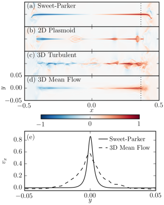
Figure 5: Comparison of outflow ($v_{x}$) profiles. (a) 2D Sweet-Parker reconnection at $t=4.2$; (b) 2D plasmoid-dominated reconnection at $t=2.6$; (c) slice of 3D turbulent reconnection at $z=0$; and (d) the mean field $\bar{v_{x}}$ of the 3D turbulent reconnection at $t=3.5$. The reconnected fluxes at the selected snapshots are approximately the same to make a fair comparison. Panel (e) shows one-dimensional cuts of the outflow profiles along the dotted lines in panel (a) and panel (d); the 3D mean flow is considerably broader than the Sweet-Parker outflow.

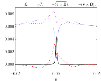
Figure 6: Decomposition of the out-of-plane mean electric field $\bar{E_{z}}$, taken at $t=3.5$ and averaged over the range from $x=-0.05$ to $x=0.05$.

Magnetic reconnection converts magnetic energy into plasma kinetic energy by turning plasma from upstream regions into Alfvénic outflow jets, which also transport plasma from upstream regions to downstream regions. It is therefore illuminating to compare the outflow profile $v_{x}$ from three simulations, shown in Figure 5. In order to make a fair comparison, these snapshots are taken at times when the reconnected magnetic fluxes are approximately the same for the three cases. Panel (a) shows the laminar, bi-directional Sweet-Parker outflow jets. In panel (b), some well-defined plasmoids are clearly visible. Panel (c) shows a $x-y$ slice at $z=0$ for the 3D run, at $t=3.5$ when turbulent reconnection is fully developed. Here some coherent structures similar to the plasmoids in panel (b) are still visible, but the structures are less regular. However, as we average over the $z$ direction to obtain the mean flow $\bar{v_{x}}$, shown in panel (d), it appears similar to a “blurred” Sweet-Parker outflow profile as in panel (a). One-dimensional cuts of the outflow profiles at the exhaust regions along the dotted lines in panel (a) and panel (c), shown in panel (e), further reinforce this impression. The mean outflow jet of 3D turbulent reconnection is substantially broader than the Sweet-Parker outflow. The ratio between the areas below the two curves, which measure the total outflow fluxes, is consistent with the enhancement of reconnection rate obtained from the magnetic flux measurement.

Because reconnection of the mean magnetic field must be driven by an out-of-plane mean electric field $\bar{E_{z}}$, it is useful to decompose $\bar{E_{z}}$ into contributions from various terms:

$$\bar{E_{z}}=-(\bar{\mathbf{v}}\times\bar{\mathbf{B}})_{z}-\overline{(\tilde{\mathbf{v}}\times\tilde{\mathbf{B}})}_{z}+\eta\bar{J_{z}},$$ (5)

where $-\overline{(\tilde{\mathbf{v}}\times\tilde{\mathbf{B}})}_{z}$ is the turbulent emf (electromotive force). Figure 6 shows an 1D cut of the decomposition along the inflow ($y)$ direction. Here each term in Eq. (5) has been averaged over the range $-0.05\leq x\leq 0.05$ to further reduce the fluctuations. These curves show that in the outer region, $\bar{E_{z}}$ is mostly balanced by the $-(\bar{\mathbf{v}}\times\bar{\mathbf{B}})_{z}$ term, whereas in the inner region, $\bar{E_{z}}$ is balanced by the resistive term $\eta\bar{J}_{z}$ and the turbulent emf term $-\overline{(\tilde{\mathbf{v}}\times\tilde{\mathbf{B}})}_{z}$. Note that $\eta\bar{J}_{z}$ is only significant in the innermost narrow region, whereas the turbulent emf covers a much wider region. Interestingly, we find that the current sheet width of mean field $\bar{J_{z}}$ is approximately the same as the corresponding Sweet-Parker current sheet width, which also manifests in the fact that $\eta\bar{J_{z}}\simeq 0.004$ at the center is approximately the same as the Sweet-Parker reconnection rate. Whether this is a general feature or simply a coincidence is not clear at this point, and should be examined in the future with simulations of higher Lundquist numbers. Nonetheless, our result indicates that although turbulence is effective in broadening the mean field outflow jets (relative to Sweet-Parker reconnection), it is less effective in broadening the mean field current sheet, if at all. This finding suggests that the effect of turbulence does not lead to an enhanced anomalous resistivity, which requires that $-\overline{(\tilde{\mathbf{v}}\times\tilde{\mathbf{B}})}_{z}$ be proportional to $\bar{J_{z}}$, but whether it may be describable in terms of hyper-resistivity (Bhattacharjee & Hameiri, 1986; van Ballegooijen & Cranmer, 2008) is left to future work.

From these analyses, we conclude that 3D turbulence enhances reconnection rate by effectively broadening the reconnection layer and outflow jets, where the turbulent emf provides important contribution to the reconnecting electric field. This picture of 3D turbulent reconnection is quite different from 2D plasmoid-dominated reconnection. In the 2D case, the reconnection rate is sped up because plasmoid instabilities cause secondary current sheets to become shorter and narrower. Reconnection takes place at multiple sites with enhanced local reconnection rates, which transport magnetic flux and plasma into plasmoids. Finally, reconnected magnetic flux and plasma are transported to the downstream region when plasmoids are ejected from the reconnection layer, typically at a Alfvénic time scale (Günter et al., 2015).

3.2 Characteristics of the Self-Sustained Turbulence

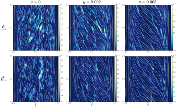
Figure 7: Energy fluctuations $\tilde{E_{k}}$ (first row) and $\tilde{E_{m}}$ (second row) at three different $x-z$ slices, overlaid with stream lines of the in-plane component of the magnetic field. These snapshots are taken at $t=3.5$, when turbulence in the reconnection layer has fully developed. The energy fluctuations form cigar-shaped eddies elongated along the direction of local magnetic field, which is one of the hallmarks of MHD turbulence.

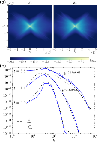
Figure 8: (a) Kinetic and magnetic energy spectra in Fourier space, integrated over the range from $y=-0.05$ to $0.05$ at $t=3.5$. Both spectra are qualitatively similar and highly anisotropic. Fourier modes are mostly excited within the region $\left|k_{x}\right|\gtrsim\left|k_{z}\right|$, as dictated by the resonant condition $\mathbf{k}\cdot\mathbf{B}\simeq 0$. (b) One-dimensional spectra at $t=0.9$, $t=1.1$, and $t=3.5$ obtained by integrating over the azimuthal direction on the $k_{x}-k_{z}$ plane.

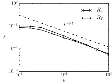
Figure 9: Eddy turnover times estimated by scale-dependent e-folding decay times of autocorrelation functions $R_{v}(k,\tau)$ and $R_{B}(k,\tau)$.

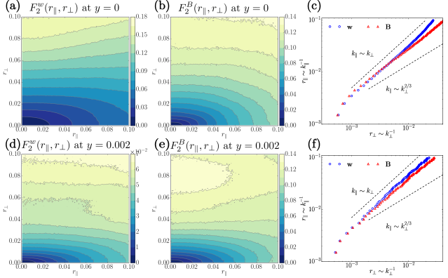
Figure 10: Two-point structure functions of the fully developed turbulence at $t=3.5$. (a) $F_{2}^{w}(r_{\parallel},r_{\perp})$ and (b) $F_{2}^{B}(r_{\parallel},r_{\perp})$ at $y=0$. (c) Relationships between semi-major axis $r_{\parallel}\sim k_{\parallel}^{-1}$ and semi-minor axis $r_{\perp}\sim k_{\perp}^{-1}$ of contours in (a) and (b), which measure the scale dependency of turbulent eddy anisotropy. The two dashed lines represent the relations $k_{\parallel}\sim k_{\perp}$ (scale-independent) and $k_{\parallel}\sim k_{\perp}^{2/3}$ (GS theory), for reference. Panels (d) – (f) are the same as panels (a) – (c), except at $y=0.002$.

Now we examine further the characteristics of the self-sustained turbulent state within the reconnection layer and make comparison with the Goldreich & Sridhar theory of incompressible MHD turbulence (Goldreich & Sridhar, 1995, 1997). In the following discussion we present detailed diagnostics of the turbulent state at $t=3.5$, but the characteristics we find here are generally valid during the period when the turbulence has fully developed, after $t=3.0$.

The first feature we notice is that the turbulent state is highly inhomogeneous — the mean magnetic field is strongly sheared over a short distance from $y=-0.002$ to $y=0.002$ (i.e. the mean field current sheet width, see Figure 6), and the turbulence is embedded in a mean flow which is also highly sheared (Figure 5 (d)). Figure 7 shows the kinetic and magnetic energy fluctuations, overlaid with streamlines of the in-plane component of the magnetic field, on three representative $x-z$ slices at the midplane $(y=0)$, the edge of the mean field current sheet ($y=0.002$), and a further outer region ($y=0.005$). These energy fluctuations form cigar-shaped eddies elongated along the direction of local magnetic field, which is one of the hallmarks of MHD turbulence. It is observed that the eddies become more elongated away from the midplane, likely because the magnetic field becomes less sheared in those regions. Fluctuations are strongest near the midplane, where the dominant magnetic field is guide field component $B_{z}\simeq 1$, and the dominant flow component is the outflow jet $v_{x}$, which can be up to the Alfvén speed $V_{A}\simeq 1$. At the midplane, the root-mean-square (RMS) values of magnetic field fluctuations $\tilde{B_{x}}$, $\tilde{B_{y}}$, and $\tilde{B_{z}}$ are approximately $0.22$, $0.05$, and $0.07$, whereas the RMS values of $\tilde{v_{x}}$, $\tilde{v_{y}}$, and $\tilde{v_{z}}$ are approximately 0.16, 0.02, and 0.05, respectively. However, as can be seen from Figure 7, fluctuations $\tilde{B}$ and $\tilde{v}$ can locally be as high as $O(1)$ of the guide field and the Alfvén speed $V_{A}$.

A common feature of turbulent systems is the formation of an extended power-law inertial range in energy spectra through cascade, which is what we will examine next. However, because our turbulent system is spatially inhomogeneous, a proper measurement of energy spectra is a challenge. The procedure we adopt is as follows. Because our primary interest is the turbulence within the reconnection layer, we multiply the fluctuating fields $\tilde{\mathbf{B}}$ and $\tilde{\mathbf{w}}$ by a $C^{\infty}$ Planck-taper window function (McKechan et al., 2010) which equals unity within the range $-0.2\leq x\leq 0.2$ and tapers off smoothly to zero over the ranges where $0.2\leq\left|x\right|\leq 0.4$. This step effectively filters out the energy fluctuations in the downstream regions which may be of different characteristics. We then calculate the discrete Fourier energy spectra of $\tilde{E_{k}}$ and $\tilde{E_{m}}$ using the “windowed” variables on each $x-z$ plane to obtain 2D energy spectra in terms of wave numbers $k_{x}$ and $k_{z}$. Finally, we integrate the 2D energy spectra over $-0.05\leq y\leq 0.05$, which is the direction of the strongest inhomogeneity. The resulting 2D spectra of $\tilde{E_{k}}$ and $\tilde{E_{m}}$ as functions of $k_{x}$ and $k_{z}$ are shown in Figure 8 (a). It can be seen that the spectra of $\tilde{E_{k}}$ and $\tilde{E_{m}}$ are qualitatively similar, and both lie predominantly in the regions where $\left|k_{x}\right|\gtrsim\left|k_{z}\right|$. This is a consequence of the fact that the energy fluctuations tend to align preferentially with local magnetic field, i.e. $\mathbf{k}\cdot\mathbf{B}\simeq 0$, whereas $B_{z}\simeq 1$ and $B_{x}$ varies approximately from $-1$ to $1$ in the reconnection layer. Although these energy spectra are anisotropic, we may still calculate 1D spectra by integrating over the azimuthal direction on the $k_{x}-k_{z}$ plane. Figure 8 (b) shows the resulting 1D spectra of $\tilde{E_{k}}$ and $\tilde{E_{m}}$, both of which exhibit an extended inertial range with a power-law spectrum $\sim k^{-\alpha}$. The kinetic energy spectrum is slightly steeper than the magnetic energy spectrum in the inertial range. During the period from $t=3.0$ to $4.8$ when the turbulence has fully developed, the power-law index $\alpha$ is typically within the range $2.1<\alpha<2.3$ for $\tilde{E_{m}}$, and $2.3<\alpha<2.5$ for $\tilde{E_{k}}$. One-dimensional power-law spectra with similar power indices are also obtained by integrating over either $k_{x}$ or $k_{z}$ directions. Figure 8 (b) also shows the 1D spectra at $t=0.9$ and $t=1.1$ when the instabilities are still in early stages of development. It shows that the instabilities initially inject energy predominantly in intermediate wave numbers $k\sim 30$ – $100$, which gradually cascades down to smaller scales (high-$k$ modes) and form the inertial range, while at the same time also develops coherent structures at larger scales, manifested as low-$k$ modes in the spectra.

Eddy turnover times at different length scales can be estimate by calculating scale-dependent autocorrelation time of relevant variables. Specifically, we calculate $R_{v}(k,\tau)\equiv\int d^{3}x\tilde{\mathbf{v}}_{k}^{>}(\mathbf{x},t)\cdot\tilde{\mathbf{v}}_{k}^{>}(\mathbf{x},t+\tau)$ and $R_{B}(k,\tau)\equiv\int d^{3}x\tilde{\mathbf{B}}_{k}^{>}(\mathbf{x},t)\cdot\tilde{\mathbf{B}}_{k}^{>}(\mathbf{x},t+\tau)$, where $\tilde{\mathbf{B}}_{k}^{>}$ and $\tilde{\mathbf{v}}_{k}^{>}$ denote high-pass filtered $\tilde{\mathbf{B}}$ and $\tilde{\mathbf{v}}$ with wavenumbers $k_{x}$ and $k_{z}$ satisfying the condition $k_{x}^{2}+k_{z}^{2}>k^{2}$, and the integrals are carried out over the region $-0.05\leq y\leq 0.05$. It is found that $R_{v}(k,\tau)$ and $R_{B}(k,\tau)$ both approximately decay exponentially with $\tau$ over a broad range of length scales set by the wavenumber $k$. This allows us to calculate scale-dependent e-folding decay times as proxies for eddy turnover times, and the results are shown in Figure 9. We find that both autocorrelation functions $R_{v}(k,\tau)$ and $R_{B}(k,\tau)$ give similar estimates for the eddy turnover time $\tau_{k}$, which approximately follow a $\tau_{k}\sim k^{-0.7}$ power law for $k\gtrsim 30$, while $\tau_{k}\simeq 0.1$ at the largest scales. Once the characteristic time scales have been established, we may further examine the validity of our convention of using an average over $z$ for the mean field by comparing with results from using a time average for the mean field. Here the interval for time averaging has to be sufficiently longer than the eddy turnover times at all scales, while sufficiently shorter than the evolution time scales of large-scale magnetic field. We have calculated the fluctuation energy spectra using an interval $\Delta t=0.275$ for time averaging, and indeed the results are similar to that in Figure 8.

To further investigate the alignment of energy fluctuations with local magnetic field, we calculate two-point structure functions in terms of parallel displacement $r_{\parallel}$ and perpendicular displacement $r_{\perp}$ with respect to local magnetic field, i.e. $F_{2}^{w}(r_{\parallel},r_{\perp})\equiv\left\langle\left|\mathbf{w}(\mathbf{x}+\mathbf{r})-\mathbf{w}(\mathbf{x})\right|^{2}\right\rangle$ and likewise $F_{2}^{B}(r_{\parallel},r_{\perp})\equiv\left\langle\left|\mathbf{B}(\mathbf{x}+\mathbf{r})-\mathbf{B}(\mathbf{x})\right|^{2}\right\rangle$. Here we adopt the procedure of Cho & Vishniac (2000), but with some modifications. Because our system is strongly inhomogeneous along the $y$ direction, the structure functions increase rapidly as the displacement $\mathbf{r}$ moves along the $y$ direction. Therefore, we calculate the structure functions for each $x-z$ plane, instead of using the full 3D space; i.e. we only allow in-plane displacement with $\mathbf{r}\cdot\hat{\mathbf{y}}=0$. Following Cho & Vishniac (2000), the local magnetic field is defined as the averaged field from the two points. However, to be consistent with the allowed displacement, the parallel and perpendicular components of the displacement are measured with respect to the in-plane component of the local magnetic field. We compute the structure functions by averaging over $10^{9}$ random pairs of points, whose $x$ coordinates are within the current sheet region $-0.25\leq x\leq 0.25$. The resulting $F_{2}^{w}(r_{\parallel},r_{\perp})$ and $F_{2}^{B}(r_{\parallel},r_{\perp})$ are shown in Figure 10 panels (a) and (b) for $y=0$, and panels (d) and (e) for $y=0.002$, where the contours reflect the shapes of eddies. These structure functions clearly show turbulent eddies elongated along the local magnetic field direction, with eddies at the $y=0.002$ plane more elongated than eddies at the midplane $y=0$. These conclusions are qualitatively consistent with earlier visual observation of Figure 7. The contours of the structure function $F_{2}^{w}(r_{\parallel},r_{\perp})$ can also be used to infer the parameter $\chi\equiv k_{\perp}v_{l}/k_{\parallel}V_{A}\sim r_{\parallel}(F_{2}^{w})^{1/2}/r_{\perp}V_{A}$ as an indicator of the strength of nonlinear interaction. Here the wave number parallel to the local magnetic field $k_{\parallel}$ is proportional to the semi-major axis $r_{\parallel}$ of a contour, and likewise the perpendicular wave number $k_{\perp}$ is proportional to the semi-minor axis $r_{\perp}$. Velocity fluctuation at the corresponding length scales is given by $v_{l}\sim(F_{2}^{w})^{1/2}$, as the plasma density $\rho\simeq 1$. It can be inferred from Figure 10 (a) and (d) that $\chi$ is an $O(1)$ quantity over a broad range of scales, indicating that the system is in a strongly nonlinear regime.

Structure function diagnostics also allow us to make comparison with an important prediction of the Goldreich & Sridhar (GS) theory of incompressible MHD turbulence (Goldreich & Sridhar, 1995, 1997), namely that eddies become increasingly more anisotropic at smaller scales. More precisely, GS theory predicts a scale-dependent anisotropy relation $k_{\parallel}\sim k_{\perp}^{2/3}$, which is based on the assumption of critical balance, i.e. the condition $k_{\parallel}V_{A}\sim k_{\perp}v_{l}$. The scale-dependent anisotropy relation $k_{\parallel}\sim k_{\perp}^{2/3}$ has been confirmed by Cho & Vishniac (2000) by using two-point structure function diagnostics. Here we repeat their procedure by plotting the relationship between the semi-minor axis $r_{\perp}\sim 1/k_{\perp}$ and the semi-major axis $r_{\parallel}\sim 1/k_{\parallel}$ of contours of structure functions. The results are shown in Figure 10 (c) and (d) for $y=0$ and $y=0.002$, respectively. The two dashed lines in each panel represent the relations $k_{\parallel}\sim k_{\perp}$ (scale-independent) and $k_{\parallel}\sim k_{\perp}^{2/3}$ (GS theory), for reference. In both panels, the relationships between $r_{\parallel}$ and $r_{\perp}$ appear to be more consistent with the scale-independent relation $k_{\parallel}\sim k_{\perp}$ than the GS theory $k_{\parallel}\sim k_{\perp}^{2/3}$. Therefore, we conclude that in this self-sustained turbulent system, the eddy anisotropy is nearly scale-independent.

4 Discussion and Conclusion

In conclusion, our simulation results indicate that 3D plasmoid instabilities in a reconnection layer can indeed lead to a self-sustained turbulent state. This state is qualified as turbulent because it exhibits key ingredients of turbulence, namely, energy cascade and development of an extended inertial range. In addition, an important feature of MHD turbulence, namely anisotropy of eddies with respect to local magnetic field, is also observed. However, the turbulent state is also highly inhomogeneous, therefore the applicability of conventional MHD turbulence theories or phenomenologies becomes questionable. In particular, we find the eddy anisotropy to be nearly scale-independent, in contrast to the prediction of $k_{\parallel}\sim k_{\perp}^{2/3}$ by the Goldreich & Sridhar theory. This discrepancy may be attributed to several factors: (1) The background field is strongly sheared. In our simulation the mean magnetic field rotates approximately 90 degrees across the reconnection layer, whereas most MHD turbulent theories assume the presence of a strong uniform guide field or no guide field at all. (2) Difference in the mechanism of energy cascade. In the present case current sheet fragmentation caused by plasmoid instabilities may play important roles in energy cascade, whereas conventional MHD turbulence theories usually assume that energy cascade is caused by interaction between counter propagating Alfvén waves. (3) The turbulence is embedded in bi-directional Alfvénic mean outflow jets, therefore disturbances in the reconnection layer will be ejected in Alfvénic time scales. This distinct feature may interfere with the energy cascade process and could be the reason why the inertial range power-law spectra in our simulation are steeper than in most homogeneous MHD turbulence situations. These considerations suggest the necessity to develop new phenomenologies to account for this type of turbulence that spontaneously arises in a reconnection layer. Recent theoretical work (Terry et al., 2012) suggests that energy spectrum in inhomogeneous turbulence driven by instabilities may not be a pure power law, but a power law multiplied by an exponential fall-off. We are currently investigating whether our numerical results can be better explained by this new theoretical framework.

In the present study, we find that once fully developed, 3D turbulent reconnection rate is similar to 2D plasmoid-dominated reconnection rate ($\sim 0.01V_{A}B$), which is approximately an order of magnitude slower than the fastest rate reported in an earlier study where turbulence is driven by external forcing (Kowal et al., 2009). Even though the scenarios of speeding up reconnection in 2D and 3D appear to be quite different, the fact that they achieve approximately similar reconnection rate is an encouraging finding and certainly needs to be further examined in simulations with higher Lundquist numbers. At the present time it has been relatively well-established that the reconnection rate in 2D plasmoid-dominated reconnection is nearly independent of the Lundquist number $S$. This conclusion is supported by heuristic arguments and has been numerically tested for a wide range of Lundquist numbers up to $S=10^{7}$ (Huang & Bhattacharjee, 2010; Uzdensky et al., 2010; Loureiro et al., 2012; Huang & Bhattacharjee, 2012, 2013). Whether this conclusion remains valid in 3D is an important open question, left to future work. A related important question is how fragmented current sheet widths scale with resistivity $\eta$. In 2D the fragmented current sheet widths follow a steep scaling $\delta\sim\eta$ such that the electric field in secondary current sheets $\sim\eta B/\delta$ and becomes independent of $\eta$. This is in fact the main argument why 2D plasmoid-dominated reconnection rate becomes independent of $\eta$ (Huang & Bhattacharjee, 2010, 2013). It becomes less clear whether this feature will persist in the case of 3D turbulent reconnection as the turbulent emf plays an important role in supporting the reconnecting electric field. As has been discussed in the context of the reconnection phase diagram by several authors (Huang et al., 2011; Ji & Daughton, 2011; Cassak & Drake, 2013), the scaling of secondary current sheet widths may potentially impact the criterion for transition from collisional to collisionless reconnection, as transition typically takes place when the current sheet width becomes smaller than kinetic scales such as ion skin depth or ion gyro radius.

Even though the scaling of secondary current sheet widths and the criterion for transition from collisional to collisionless reconnection are uncertain at the present time, it is likely that in some astrophysical applications dissipation may take place at kinetic scales as turbulence cascades down to smaller scales. An important question is: will kinetic physics at small scales feed back to large scales and alter the conclusion from MHD simulations? Comparing our MHD results with those obtained from collisionless particle-in-cell (PIC) simulation (Daughton et al., 2011), we note that oblique tearing modes play a similar role in developing self-generated turbulent reconnection in both cases. A more recent study (Daughton et al., 2014) also shows that 2D and 3D PIC simulations yield similar reconnection rates. A noticeable difference between the MHD and PIC simulations is the aspect ratio of turbulent region. The turbulent region in PIC simulation is considerably broader, whereas that in MHD simulation is more elongated. However, 3D PIC simulations are limited to relative small system sizes typical of tens of ion skin depths, therefore lack sufficient separation between large and small scales. It remains an open question how the aspect ratio of the turbulent region may change as collisionless PIC simulations scale up to larger system sizes.

In recent years, there have been attempts to determine post-CME (coronal mass ejection) current sheet thickness by using UVCS (UltraViolet Coronagraph Spectrometer) and LASCO (Large Angle and Spectrometric Coronagraph) observations (Ciaravella & Raymond, 2008; Lin et al., 2009). These studies usually find the current sheet thickness to be significantly broader than classical or anomalous resistivity would predict, and turbulence has been suggested as a possible explanation. Using UVCS observation for the 2003 November 4 CME event, Ciaravella & Raymond (2008) estimate the current sheet thickness to be within the range $0.04$ – $\mbox{0.08}R_{\odot}$ at lower latitude ($\sim 1.5R_{\odot}$), whereas the current sheet length may be estimated from LASCO images as approximately $4R_{\odot}$. That gives an estimate of the aspect ratio to be within the range $50$ – $100$. The study by Lin et al. (2009) also finds similar current sheet thickness at lower latitude for other events, while the thickness tends to increase at higher latitude. Taking this into account, the estimated aspect ratio ($50$ – $100$) should be regarded as an upper bound. It should be noted that neither UVCS nor LASCO measure the electric current density directly; instead, they measure the temperature or density enhancement in the sheet-like structure. If we assume the observed thickness is a consequence of turbulence (e.g. due to turbulence heating and mixing), preliminary comparison may be made with our simulation results. In the fully developed turbulent state of our simulation, the thickness of the turbulent region is approximately $0.02$ (Figure 3) while the reconnection layer length is approximately $0.8$, therefore the aspect ratio is approximately $40$, which is not inconsistent with the estimated aspect ratio from UVCS observation. We should point out that our simulation and above mentioned post-CME current sheets are of very different global configurations and plasma parameter regimes, and important effects such as plasma heating and thermal conduction are not included in our model, therefore a direct comparison may not be possible. Future work is needed to further assess whether turbulent broadening can account for the observed thickness of post-CME sheet-like structure.

References

- Baalrud et al. (2012) Baalrud, S. D., Bhattacharjee, A., & Huang, Y.-M. 2012, Phys. Plasmas, 19, 022101
- Balbus & Hawley (1998) Balbus, S. A., & Hawley, J. F. 1998, Rev. Mod. Phys., 70, 1
- Bárta et al. (2011) Bárta, M., Büchner, J., Karlický, M., & Skála, J. 2011, Astrophys. J., 737, 24
- Bhattacharjee & Hameiri (1986) Bhattacharjee, A., & Hameiri, E. 1986, Phys. Rev. Lett., 57, 206
- Bhattacharjee et al. (2009) Bhattacharjee, A., Huang, Y.-M., Yang, H., & Rogers, B. 2009, Phys. Plasmas, 16, 112102
- Biskamp (1986) Biskamp, D. 1986, Phys. Fluids, 29, 1520
- Biskamp (2000) —. 2000, Magnetic Reconnection in Plasmas (Cambridge University Press)
- Cassak & Drake (2013) Cassak, P. A., & Drake, J. F. 2013, Phys. Plasmas, 20, 061207
- Cassak et al. (2009) Cassak, P. A., Shay, M. A., & Drake, J. F. 2009, Phys. Plasmas, 16, 120702
- Cho & Vishniac (2000) Cho, J., & Vishniac, E. T. 2000, Astrophys. J., 539, 273
- Ciaravella & Raymond (2008) Ciaravella, A., & Raymond, J. C. 2008, Astrophys. J., 686, 1372
- Daughton et al. (2014) Daughton, W., Nakamura, T. K. M., Karimabadi, H., Roytershteyn, V., & Loring, B. 2014, Phys. Plasmas, 21, 052307
- Daughton et al. (2009) Daughton, W., Roytershteyn, V., Albright, B. J., et al. 2009, Phys. Rev. Lett., 103, 065004
- Daughton et al. (2011) Daughton, W., Roytershteyn, V., Karimabadi, H., et al. 2011, Nature Physics, 7, 539
- Daughton et al. (2006) Daughton, W., Scudder, J., & Karimabadi, H. 2006, Phys. Plasmas, 13, 072101
- Eyink et al. (2011) Eyink, G. L., Lazarian, A., & Vishniac, E. T. 2011, Astrophys. J., 743, 51
- Fermo et al. (2012) Fermo, R. L., Drake, J. F., & Swisdak, M. 2012, Phys. Rev. Lett., 108, 255005
- Frisch (1995) Frisch, U. 1995, Turbulence: the legacy of A. N. Kolmogorov (Cambridge University Press)
- Goldreich & Sridhar (1995) Goldreich, P., & Sridhar, S. 1995, Astrophys. J., 438, 763
- Goldreich & Sridhar (1997) —. 1997, Astrophys. J., 485, 680
- Günter et al. (2015) Günter, S., Yu, Q., Lackner, K., Bhattacharjee, A., & Huang, Y.-M. 2015, Plasma Phys. Control. Fusion, 57, 014017
- Guzdar et al. (1993) Guzdar, P. N., Drake, J. F., McCarthy, D., Hassam, A. B., & Liu, C. S. 1993, Phys. Fluids B, 5, 3712
- Huang & Bhattacharjee (2010) Huang, Y.-M., & Bhattacharjee, A. 2010, Phys. Plasmas, 17, 062104
- Huang & Bhattacharjee (2012) —. 2012, Phys. Rev. Lett., 109, 265002
- Huang & Bhattacharjee (2013) —. 2013, Phys. Plasmas, 20, 055702
- Huang et al. (2014) Huang, Y.-M., Bhattacharjee, A., & Boozer, A. H. 2014, Astrophys. J., 793, 106
- Huang et al. (2011) Huang, Y.-M., Bhattacharjee, A., & Sullivan, B. P. 2011, Phys. Plasmas, 18, 072109
- Ji & Daughton (2011) Ji, H., & Daughton, W. 2011, Phys. Plasmas, 18, 111207
- Kida & Orszag (1992) Kida, S., & Orszag, S. A. 1992, Journal of Scientific Computing, 7, 1
- Kowal et al. (2009) Kowal, G., Lazarian, A., Vishniac, E. T., & Otmianowska-Mazur, K. 2009, Astrophys. J., 700, 63
- Lapenta (2008) Lapenta, G. 2008, Phys. Rev. Lett., 100, 235001
- Lazarian et al. (2015a) Lazarian, A., Eyink, G., Vishniac, E., & Kowal, G. 2015a, Proc. R. Soc. A, 373, 20140144
- Lazarian et al. (2012a) Lazarian, A., Eyink, G. L., & Vishniac, E. T. 2012a, Phys. Plasmas, 19, 012105
- Lazarian et al. (2015b) Lazarian, A., Eyink, G. L., Vishniac, E. T., & Kowal, G. 2015b, in Magnetic Fields in Diffuse Media, ed. A. Lazarian, E. M. de Gouveia Dal Pino, & C. Melioli (Springer-Verlag Berlin Heidelberg), 311–372
- Lazarian & Vishniac (1999) Lazarian, A., & Vishniac, E. T. 1999, Astrophys. J., 517, 700
- Lazarian et al. (2012b) Lazarian, A., Vlahos, L., Kowal, G., et al. 2012b, Space Sci. Rev., 173, 557
- Lin et al. (2009) Lin, J., Li, J., Ko, Y.-K., & Raymond, J. C. 2009, Astrophys. J., 693, 1666
- Loureiro et al. (2012) Loureiro, N. F., Samtaney, R., Schekochihin, A. A., & Uzdensky, D. A. 2012, Phys. Plasmas, 19, 042303
- Loureiro et al. (2007) Loureiro, N. F., Schekochihin, A. A., & Cowley, S. C. 2007, Phys. Plasmas, 14, 100703
- Loureiro et al. (2009) Loureiro, N. F., Uzdensky, D. A., Schekochihin, A. A., Cowley, S. C., & Yousef, T. A. 2009, Mon. Not. R. Astron. Soc., 399, L146
- McKechan et al. (2010) McKechan, D. J. A., Robinson, C., & Sathyaprakash, B. S. 2010, Class. Quantum Grav., 27, 084020
- Narayan (1992) Narayan, R. 1992, Phil. Trans. R. Soc. A, 341, 151
- Ni et al. (2012) Ni, L., Ziegler, U., Huang, Y.-M., Lin, J., & Mei, Z. 2012, Phys. Plasmas, 19, 072902
- Parker (1957) Parker, E. N. 1957, J. Geophys. Res., 62, 509
- Parker (1988) —. 1988, Astrophys. J., 330, 474
- Petschek (1964) Petschek, H. E. 1964, in AAS/NASA Symposium on the Physics of Solar Flares, ed. W. N. Hess (Washington, DC: NASA), 425
- Priest & Forbes (2000) Priest, E. R., & Forbes, T. 2000, Magnetic reconnection : MHD theory and applications (Cambridge University Press)
- Rappazzo et al. (2010) Rappazzo, A. F., Velli, M., & Einaudi, G. 2010, Astrophys. J., 722, 65
- Rappazzo et al. (2008) Rappazzo, A. F., Velli, M., Einaudi, G., & Dahlburg, R. B. 2008, Astrophys. J., 677, 1348
- Rickett (1990) Rickett, B. J. 1990, Annu. Rev. Astron. Astrophys., 28, 561
- Servidio et al. (2009) Servidio, S., Matthaeus, W. H., Shay, M. A., Cassak, P. A., & Dmitruk, P. 2009, Phys. Rev. Lett., 102, 115003
- Servidio et al. (2010) Servidio, S., Matthaeus, W. H., Shay, M. A., et al. 2010, Phys. Plasmas, 17, 032315
- Servidio et al. (2011) Servidio, S., Dmitruk, P., Greco, A., et al. 2011, Nonlin. Processes Geophys., 18, 675
- Shen et al. (2011) Shen, C., Lin, J., & Murphy, N. A. 2011, Astrophys. J., 737, 14
- Shepherd & Cassak (2010) Shepherd, L. S., & Cassak, P. A. 2010, Phys. Rev. Lett., 105, 015004
- Shibata & Tanuma (2001) Shibata, K., & Tanuma, S. 2001, Earth Planets Space, 53, 473
- Sweet (1958) Sweet, P. A. 1958, in Electromagnetic phenomena in cosmical physics, ed. B. Lehnert, Vol. 6 (Cambridge University Press), 123–134
- Takamoto (2013) Takamoto, M. 2013, Astrophys. J., 775, 50
- Terry et al. (2012) Terry, P. W., Almagri, A. F., Fiksel, G., et al. 2012, Phys. Plasmas, 19, 055906
- Uzdensky et al. (2010) Uzdensky, D. A., Loureiro, N. F., & Schekochihin, A. A. 2010, Phys. Rev. Lett., 105, 235002
- van Ballegooijen & Cranmer (2008) van Ballegooijen, A. A., & Cranmer, S. R. 2008, Astrophys. J., 682, 644
- Wan et al. (2014) Wan, M., Rappazzo, A. F., Matthaeus, W. H., Servidio, S., & Oughton, S. 2014, Astrophys. J., 797, 63
- Wyper & Hesse (2015) Wyper, P. F., & Hesse, M. 2015, Phys. Plasmas, 22, 042117
- Wyper & Pontin (2014) Wyper, P. F., & Pontin, D. I. 2014, Phys. Plasmas, 21, 082114
- Yamada et al. (2010) Yamada, M., Kulsrud, R., & Ji, H. 2010, Rev. Mod. Phys., 82, 603
- Zweibel & Yamada (2009) Zweibel, E. G., & Yamada, M. 2009, Annu. Rev. Astron. Astrophys., 47, 291