Controlling statistical moments of stochastic dynamical networks

Abstract

We consider a general class of stochastic networks and ask which network nodes need to be controlled, and how, to stabilize and switch between desired metastable (target) states in terms of the first and second statistical moments of the system. We first show that it is sufficient to directly interfere with a subset of nodes which can be identified using information about the graph of the network only. Then, we develop a suitable method for feedback control which acts on that subset of nodes and preserves the covariance structure of the desired target state. Finally, we demonstrate our theoretical results using a stochastic Hopfield network and a global brain model. Our results are applicable to a variety of (model) networks, and further our understanding of the relationship between network structure and collective dynamics for the benefit of effective control.

I Introduction

Complex dynamical network models are widely applied in science and engineering to describe and examine various natural and human-produced phenomena. Examples include models of neuronal networks, gene regulatory networks, financial networks, social networks, power grids and highway webs Newman (2003); Boccaletti2006. Noise is often included to reflect the variability observed in the real system; therefore, stochastic dynamical networks constitute a particularly relevant model class.

Of great interest are the relationships between the structural properties of the network (i.e., properties of its graph) and the network dynamics – in particular, stochastic synchronization phenomena and their controllability Glass2001; Neiman1999; Zaks2005; Zhou2005; Porfiri2008; Wang2010. In human neuroscience, for example, the zero-lag correlations between measured fluctuating (neuronal) activities of different brain areas reveal functional connectivity patterns and can thereby serve as a biomarker for a number of brain diseases Fox2005; Damoiseaux2006; Rosazza2011 These connectivity patterns are strongly influenced, but not fully determined, by the brain network graph Haimovici2013; Deco2013JN; Deco2013TINS.

In this contribution, we ask whether and how the first and second statistical moments of stochastic dynamical networks can be controlled in general by directly interfering only with a subset of nodes. These nodes should be determined using solely information about the network graph. Specifically, we consider a general class of stochastic dynamical network models which possess a set of collective equilibrium states in terms of steady-state mean values of node variables and covariance patterns. The aim is to switch between these network states by pinning only a subset of nodes in an appropriate way. That is, we consider pinning control (also known as clamping control) and examine the capabilities of the pinned nodes to hold the means for the free nodes and the covariances between them at the desired equilibrium values.

Our approach consists of three steps (see Fig. 1): First, we describe the dynamics of the first and second moments of the stochastic network system by a closed system of coupled ordinary differential equations using a method of moments (Section II). Based on the graph of that deterministic system we then identify subsets of moments, which, when controlled, steer the dynamics of the whole moments system to a desired metastable state (Section III). Since the graph of the system that describes the dynamics of the moments differs from the graph of the underlying network system, we next determine the subset of nodes that need to be controlled in the original network (same section). In the last step we design a feedback controller that acts on the determined subset of nodes of the stochastic network system to switch between correlation patterns (Section IV). We demonstrate the applicability of our theoretical results using two example models: i) a noisy Hopfield network – a well-studied class of recurrent neural network models (Section V) and ii) a calibrated global brain network (Section VI). Limitations of the developed method and possible adjustments are discussed in Section VII.

II Stochastic network model and the moments system

Consider the network model consisting of $N$ nodes described by

$$\dot{\mathbf{x}}_{i}=\mathbf{f}_{i}(t,\mathbf{x}_{i},\mathbf{x}_{I_{i}})+\mathbf{M}_{i}\boldsymbol{\eta}_{i}(t),$$ (1)

where $\mathbf{x}_{i}(t)\in\mathbb{R}^{m_{i}}$ is the (time-varying) $m_{i}$-dimensional state vector of node $i\in\{1,\dots,N\}$, the vector field $\mathbf{f}_{i}:\mathbb{R}\times\mathbb{R}^{m_{i}}\times\mathbb{R}^{\sum_{j\neq i}m_{j}}\to\mathbb{R}^{m_{i}}$ is continuous, uniformly bounded and sufficiently differentiable, and $I_{i}$ is the set of input node indices for node $i$. $\boldsymbol{\eta}_{i}(t)$ is a $m_{i}$-dimensional Gaussian white noise process with $\langle\boldsymbol{\eta}_{i}(t)\boldsymbol{\eta}_{i}(t+\tau)^{T}\rangle=\delta(\tau)\mathbf{I}_{i}$, where $\mathbf{I}_{i}$ is the $m_{i}\times m_{i}$ identity matrix, and $\mathbf{M}_{i}$ is a constant noise mixing matrix. Equation (1) can be expressed in compact form as

$$\dot{\mathbf{x}}=\mathbf{f}(t,\mathbf{x})+\mathbf{M}\boldsymbol{\eta}(t),$$ (2)

where $\mathbf{x}\in\mathbb{R}^{k},k:=\sum_{i}m_{i}$, $\mathbf{f}(t,\mathbf{x})=[\mathbf{f}_{1}(t,\mathbf{x}_{1},\mathbf{x}_{I_{1}})^{T},\dots,\mathbf{f}_{N}(t,\mathbf{x}_{N},\mathbf{x}_{I_{N}})^{T}]^{T}$, $\mathbf{M}$ is a block matrix with blocks $\mathbf{M}_{i}$ on the main diagonal, and $\boldsymbol{\eta}(t)$ is a $k$-dimensional Gaussian white noise process. $\mathbf{f}(t,\mathbf{x})$ generates a directed graph $\Gamma$ with $N$ nodes, where the edges that connect node $i$ with its input nodes are indicated by the set $I_{i}$.

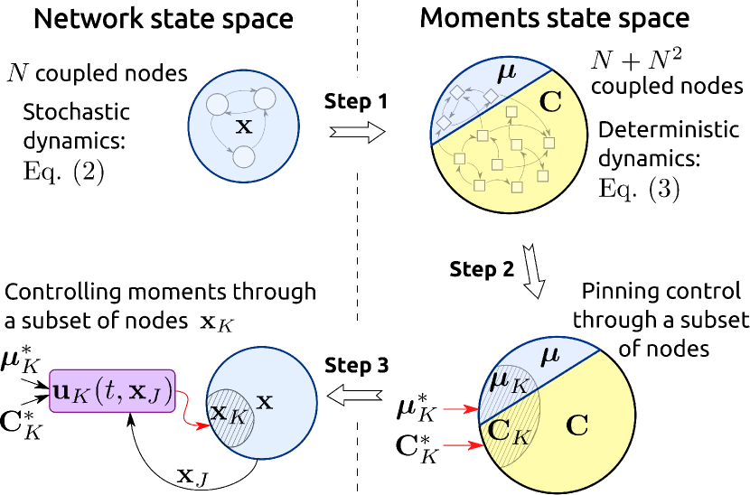
Figure 1: Schematic of the control scheme. Left: State space of the stochastic dynamical network whose state is represented by the vector $\mathbf{x}$. Right: State space of the corresponding moments $\boldsymbol{\mu}$ (mean vector) and $\mathbf{C}$ (covariance matrix) of $\mathbf{x}$, whose dynamics is governed by a deterministic system of equations. Red arrows indicate pinning control through the subsets of nodes $\boldsymbol{\mu}_{K}$, $\mathbf{C}_{K}$ and $\mathbf{x}_{K}$, respectively. $\boldsymbol{\mu}_{K}^{*}$ and $\mathbf{C}_{K}^{*}$ are the values of dynamic variables $\boldsymbol{\mu}_{K}$ and $\mathbf{C}_{K}$ on the (metastable) target state. $\mathbf{u}_{K}(t,\mathbf{x}_{J}(t))$ denotes the feedback control signal which directly affects the subset of nodes $\mathbf{x}_{K}$ and depends on the complementary subset $\mathbf{x}_{J}$.

The dynamics of the mean vector $\boldsymbol{\mu}(t):=\langle\mathbf{x}\rangle(t)$ and the covariance matrix $\mathbf{C}(t):=\mathrm{cov}(\mathbf{x},\mathbf{x})(t)=\langle(\mathbf{x}-\boldsymbol{\mu})(\mathbf{x}-\boldsymbol{\mu})^{T}\rangle(t)$ for the system Eq. 2 can be described by (deterministic) ordinary differential equations using a method of moments assuming weak noise Rodriguez1996. Employing the Fokker-Planck equation for the probability density function $p(\mathbf{x},t)$ of $\mathbf{x}$ at time $t$, integrating that equation over the state space and using second order Taylor expansion of $\mathbf{f}(t,\mathbf{x})$ with respect to $\mathbf{x}$ under the integral we obtain the moments system (MS),

$$\dot{\boldsymbol{\mu}} =\mathbf{f}(t,\boldsymbol{\mu})+\frac{1}{2}\nabla\nabla\mathbf{f}(t,\boldsymbol{\mu})\cdot\mathbf{C}$$ (3a)

$$\dot{\mathbf{C}} =\nabla\mathbf{f}(t,\boldsymbol{\mu})\mathbf{C}+\mathbf{C}\nabla\mathbf{f}(t,\boldsymbol{\mu})^{T}+\mathbf{Q},$$ (3b)

where $\nabla\mathbf{f}(t,\mathbf{x})$ is the Jacobian matrix of $\mathbf{f}$ with respect to $\mathbf{x}$ and $\mathbf{Q}:=\mathbf{M}\mathbf{M}^{T}$ is the total noise covariance matrix. Note, that

$${\left[\nabla\nabla\mathbf{f}(t,\boldsymbol{\mu})\cdot\mathbf{C}\right]_{j}=\sum_{l,p}\frac{\partial^{2}}{\partial x_{l}\partial x_{p}}\left[\mathbf{f}(t,\mathbf{x})\right]_{j}\big{|}_{\mathbf{x}=\boldsymbol{\mu}}\mathbf{C}_{lp}}$$

where $j=1,\dots,k$. The MS has a larger, $(k+k^{2})$-dimensional state space. It is convenient to consider this system as a network of $N+N^{2}$ coupled nodes. The $N$ components $\boldsymbol{\mu}_{i}(t)$ of $\boldsymbol{\mu}(t)$ describe the mean values (over noise realizations) of the stochastic network nodes, the $N$ diagonal $m_{i}\times m_{i}$ blocks of $\mathbf{C}(t)$ – variances, and the $N^{2}-N$ off-diagonal $m_{i}\times m_{j}$ blocks – covariances between these nodes. Hence, the MS generates a connectivity graph $\Gamma^{*}$, which is related to the graph $\Gamma$ via $\mathbf{f}$.

III Identifying network nodes for control

For a deterministic network model, as given by Eq. 2 without the noise term, i.e.,

$$\dot{\mathbf{x}}=\mathbf{f}(t,\mathbf{x}),$$ (4)

it is possible that only a subset of nodes needs to be pinned (i.e., prescribed to a target trajectory) in order to drive the whole system to a target solution (an attractor) Fiedler2013. These nodes are termed switching nodes (SN) and formally defined as follows:

Definition III.1.

A subset $K$ of the vertex set $I:=\{1,\dots,N\}$ for the system given by Eq. 4 is called a set of switching nodes, if

$$\lim_{t\to+\infty}\mathbf{x}_{I\setminus K}(t)=\mathbf{x}_{I\setminus K}^{*}(t)$$

holds for any solution $\mathbf{x}_{I\setminus K}(t)$ of the subsystem

$$\dot{\mathbf{x}}_{I\setminus K}=\mathbf{f}_{I\setminus K}(t,\mathbf{x}_{I\setminus K},\mathbf{x}^{*}_{K})$$

and for any solution $\mathbf{x}^{*}(t)$ of Eq. 4 (the full system).

Here, $\mathbf{x}_{I\setminus K}(t)$ denotes the joint state vector of all nodes in $I$ except the switching nodes $K$. In other words, if the SN are forced to attain the values from one of the solutions $\mathbf{x}^{*}(t)$ of the network system, the whole network is guaranteed to converge to that solution as $t\to\infty$ for all initial conditions. It should be noted that SN are a special case of the so-called determining nodes proposed in Fiedler2013. The difference is that the latter must (at least) tend to $\mathbf{x}_{K}^{*}(t)$ as $t\to\infty$, whereas the former are forced to follow $\mathbf{x}_{K}^{*}(t)$ exactly. We use SN in this work because they are powerful enough for the control purposes and simplify the mathematical derivations below.

Importantly, the set of SN can be identified based solely on the structural information of the network [i.e., knowing $\Gamma$ and not necessarily $\mathbf{f}(t,\mathbf{x})$]. The following assumptions are required:

Assumption III.1.

Dissipativity: The system without noise, Eq. 4 is dissipative, i.e., as time tends to infinity, the state of the system stays within a ball of finite radius, for all initial conditions.

Assumption III.2.

Decay condition: $\nabla_{\mathbf{x}_{i}}\mathbf{f}_{i}(t,\mathbf{x}_{i},\mathbf{x}_{I_{i}})<0$, $\forall i\in\{1,\dots,N\}$ and for all $t$ and bounded $\mathbf{x}$. In other words, the Jacobian matrix of $\mathbf{f}_{i}$ with respect to $\mathbf{x}_{i}$ is strictly negative definite.

If Assumption III.2 does not hold for a node $\mathbf{x}_{j}$, an explicit edge from the node to itself is implied in the graph $\Gamma$ (see Section 1 in Fiedler2013). With these two assumptions, the set of SN is identical to the feedback vertex set (FVS) of $\Gamma$, defined as:

Definition III.2.

A feedback vertex set of a directed graph $\Gamma$ is a possibly empty subset $K$ of vertices such that the subgraph $\Gamma\setminus K$ is acyclic.

Here, $\Gamma\setminus K$ denotes the subgraph that remains when all vertices of $K$ are removed from $\Gamma$ along with all edges from or towards those vertices. This implies that the structural information alone can provide clues about the dynamics and controllability of the system. Note, however, that the problem of finding minimal FVS of a directed graph is NP-complete Karp1972.

Let us now consider the graph $\Gamma^{*}$ of the MS, Eqs. 3a and 3b, which can be revealed by rewriting that system using block-wise notation,

$$\dot{\boldsymbol{\mu}}_{i} =\mathbf{f}_{i}+\frac{1}{2}\sum_{k,j\in\{i\}\cup I_{i}}\nabla_{j}\nabla_{k}\mathbf{f}_{i}\cdot\mathbf{C}_{kj}$$ (5a)

$$\dot{\mathbf{C}}_{ij} =\nabla_{i}\mathbf{f}_{i}\mathbf{C}_{ij}+\mathbf{C}_{ij}^{T}\nabla_{i}\mathbf{f}_{j}^{T}+\mathbf{Q}_{ij}$$

$$\quad+\sum_{k\in I_{i}}\nabla_{k}\mathbf{f}_{i}\mathbf{C}_{kj}+\sum_{k\in I_{j}}\mathbf{C}_{ik}^{T}\nabla_{k}\mathbf{f}_{j}^{T},$$ (5b)

where $\mathbf{f}_{i}$ is evaluated at $\mathbf{x}=\boldsymbol{\mu}$, i.e., $\mathbf{f}_{i}=\mathbf{f}_{i}(t,\boldsymbol{\mu}_{i},\boldsymbol{\mu}_{I_{i}})$ and $\nabla_{k}\mathbf{f}_{i}$ is the Jacobian of $\mathbf{f}_{i}$ with respect to the state vector $\mathbf{x}_{k}$, evaluated at $\mathbf{x}=\boldsymbol{\mu}$. For improved readability the dependency of $\mathbf{f}_{i}$ and its derivatives on $\boldsymbol{\mu}_{i}$ and $\boldsymbol{\mu}_{I_{i}}$ is implied and not indicated separately. Notably, the Jacobian of the right-hand side of Eq. 5a, i.e., the derivative with respect to $\boldsymbol{\mu}_{i}$, is not guaranteed to be negative definite – even if the graph $\Gamma$ of the original system does not contain cycles (i.e., the fact that the decay condition holds for $\mathbf{f}_{i}$ and $I_{i}$ does not include $i$ itself, for all $i\in I$). This implies that every node $\boldsymbol{\mu}_{i}$ of $\Gamma^{*}$ must have a self-connecting edge. Thus, the minimal FVS (Definition III.2) of $\Gamma^{*}$ includes at least all nodes $\boldsymbol{\mu}_{i}$, cf. Eq. 5a. To provide a simple example, in Fig. 2 the subgraph structure of the moments system of a network of 4 nodes with circular topology (directed ring) is visualized. Note, that in this example the minimal FVS of the original graph $\Gamma$ consists of only one node. The minimal FVS of $\Gamma^{*}$ – according to the two subgraphs – contains at least 11 nodes: $\boldsymbol{\mu}_{1},\dots,\boldsymbol{\mu}_{4}$ plus one arbitrary row and one arbitrary column of $\mathbf{C}$.

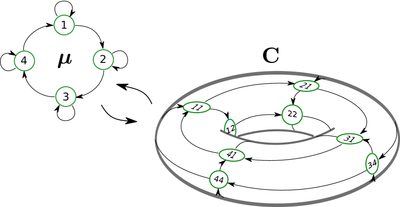
Figure 2: Subgraphs of connectivity graph $\Gamma^{*}$ of the MS (cf. Eqs. 5a and 5b) of a network (cf. Eq. 1) of $N=4$ nodes with circular graph $\Gamma$. Left: Subgraph for the connectivity of the expected value nodes $\boldsymbol{\mu}_{i}$. Right: Subgraph for the connectivity between the (co)variance nodes $\mathbf{C}_{ij}$, $i,j\in\{1,\dots,N\}$. Numbers indicate the values of the indices of $\boldsymbol{\mu}$ and $\mathbf{C}$, respectively.

However, it is possible to find a set of SN that is smaller than the minimal FVS of $\Gamma^{*}$. Using the dynamical properties of Eqs. 3a and 3b together with the structure of (any given) $\Gamma$ – under the Assumptions III.1 and III.2, and

Assumption III.3.

Weak noise: the probability $P(||\mathbf{x}(t)-\boldsymbol{\mu}(t)||<\epsilon)$ is close to $1$ for any norm $||\cdot||$ and small $\epsilon>0$.

(already assumed for the method of moments) – we obtain:

Proposition III.1.

Let $K\subseteq I$ be the minimal feedback vertex set of the graph $\Gamma$ of the stochastic system, Eq. 2, with total vertex set $I:=\{1,\dots,N\}$, and let Assumptions III.1, III.2 and III.3 hold. Then the set of switching nodes for the corresponding moments system, Eqs. 3a and 3b, is given by

$$K^{*}:=\{\boldsymbol{\mu}_{j},\mathbf{C}_{ij},\mathbf{C}_{ji}:j\in K,i\in I\}.$$ (6)

In other words, if the FVS of the stochastic system is $K$, then the set of SN $K^{*}$ of the associated MS consists of the means and variances of the nodes in $K$ and, importantly, the covariances between these nodes and all others (visualized in Fig. 3 for $K=\{2,3\}$). The set of SN of the MS for the example ring network mentioned above consists of one arbitrary mean vector $\boldsymbol{\mu}_{i}$ plus the covariances between the corresponding node ($\mathbf{x}_{i}$) and all other nodes. The proof of Eq. 6 is given in the Appendix Appendix.

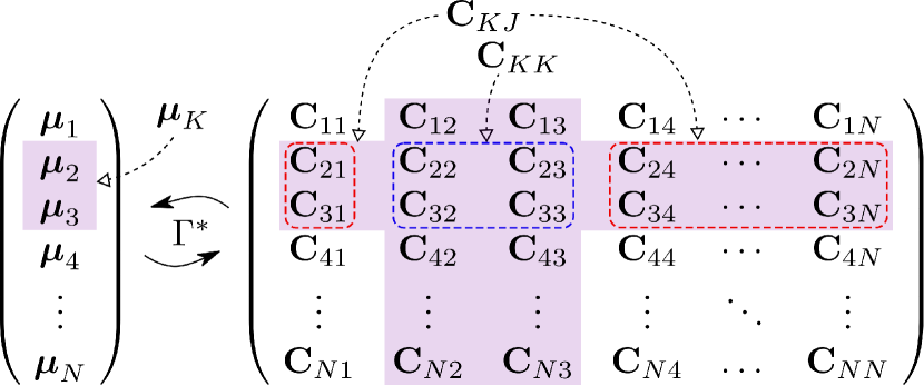
Figure 3: Schematic of mean vector $\boldsymbol{\mu}$ and covariance matrix $\mathbf{C}$, where a subset of nodes is highlighted by shaded background. That subset $K^{*}$ of nodes needs to be controlled, given that the FVS $K$ of the (original) network consists of nodes 2 and 3. In general, the set $K^{*}$ comprises the nodes $\boldsymbol{\mu}_{i}$ with the same index values as in the FVS of the original network, plus the corresponding rows and columns of the matrix $\mathbf{C}$, cf. Eq. 6.

IV Designing the controller

When controlled via pinning, the set of SN is capable to switch the entire network system from any state to the desired metastable state. According to Eq. 6, the set of SN $K^{*}$ of a MS includes the nodes that describe the covariances between the nodes of the minimal FVS $K$ with the rest of the nodes of the stochastic network system. Assuming that the nodes in $K$ are physically accessible, the question is how to choose the appropriate $\mathbf{u}_{K}(t):=\mathbf{x}_{K}(t)$ for the stochastic system such that the set of nodes $K^{*}$ of the corresponding MS are pinned (Fig. 1).

Let us consider the system given by Eq. 2, with FVS $K$, as two coupled subsystems,

$$\dot{\mathbf{x}}_{K} =\mathbf{f}_{K}(t,\mathbf{x}_{K},\mathbf{x}_{J})+\mathbf{M}_{K}\boldsymbol{\eta}_{K}(t)$$ (7a)

$$\dot{\mathbf{x}}_{J} =\mathbf{f}_{J}(t,\mathbf{x}_{J},\mathbf{x}_{K})+\mathbf{M}_{J}\boldsymbol{\eta}_{J}(t),$$ (7b)

where $J:=I\setminus K$, and $\boldsymbol{\eta}_{J}(t)$, $\boldsymbol{\eta}_{K}(t)$ are independent Gaussian white noise processes. Controlling the whole system is then reduced to controlling the subsystem, Eq. 7b, with the control signal $\mathbf{u}_{K}(t)$ that is used to pin the nodes in $K$: $\mathbf{x}_{K}(t)=\mathbf{u}_{K}(t)$ and

$$\dot{\mathbf{x}}_{J}=\mathbf{f}_{J}(t,\mathbf{x}_{J},\mathbf{u}_{K}(t))+\mathbf{M}_{J}\boldsymbol{\eta}_{J}(t).$$ (8)

Note that by definition of SN (Definition III.1), if $\boldsymbol{\eta}_{J}(t)\equiv 0$, setting the control signal to the desired (deterministic) attractor, $\mathbf{u}_{K}(t)=\mathbf{x}^{*}_{K}(t)$ guarantees that the subsystem $\mathbf{x}_{J}$ necessarily converges to the desired state $\mathbf{x}^{*}_{J}(t)$. With non-zero noise, however, we seek to guide the system to a metastable state in the moments space, that is, we want to control the expected value and covariance matrix of $\mathbf{x}(t)$ rather than the stochastic $\mathbf{x}(t)$ itself. Therefore, the goal is to design a stochastic feedback controller $\mathbf{u}_{K}(t,\mathbf{x}_{J}(t))$, such that the following conditions (in the moments space) are satisfied:

$$\langle\mathbf{u}_{K}\rangle(t)=\boldsymbol{\mu}_{K}^{*}(t)$$ (9a)

$$\mathrm{cov}(\mathbf{u}_{K},\mathbf{u}_{K})(t)=\mathbf{C}^{*}_{KK}(t)$$ (9b)

$$\mathrm{cov}(\mathbf{x}_{J},\mathbf{u}_{K})(t)=\mathbf{C}^{*}_{JK}(t)=\mathbf{C}_{KJ}^{*T}(t)$$ (9c)

where $\boldsymbol{\mu}^{*}(t)$ and $\mathbf{C}^{*}(t)$ denote the values of the target metastable state in the moments space. We choose $\mathbf{u}_{K}(t,\mathbf{x}_{J}(t))$ as a linear feedback controller of the form:

$$\mathbf{u}_{K}(t,\mathbf{x}_{J}(t)):=[\boldsymbol{\mu}_{g}(t)+\mathbf{C}_{g}^{\frac{1}{2}}(t)\boldsymbol{\eta}_{g}(t)]+\mathbf{W}(t)^{T}\mathbf{x}_{J}(t)$$ (10)

where $[\boldsymbol{\mu}_{g}(t)+\mathbf{C}_{g}^{\frac{1}{2}}(t)\boldsymbol{\eta}_{g}(t)]$ is an independent time-uncorrelated Gaussian process with mean $\boldsymbol{\mu}_{g}(t)$ and covariance $\mathbf{C}_{g}(t)$, and $\mathbf{W}(t)\in\mathbb{R}^{m_{J}\times m_{K}}$ is a feedback weighting matrix to be determined. The expected value $\boldsymbol{\mu}_{K}(t):=\langle\mathbf{x}_{K}\rangle(t)=\langle\mathbf{u}_{K}\rangle(t)$ is then given by

$$\boldsymbol{\mu}_{K}(t)=\boldsymbol{\mu}_{g}(t)+\mathbf{W}^{T}(t)\boldsymbol{\mu}_{J}(t),$$ (11)

the covariance matrix $\mathbf{C}_{KK}(t):=\mathrm{cov}(\mathbf{x}_{K},\mathbf{x}_{K})(t)=\mathrm{cov}(\mathbf{u}_{K},\mathbf{u}_{K})(t)$ reads

$$\mathbf{C}_{KK}(t)=\mathbf{C}_{g}(t)+\mathbf{W}^{T}(t)\mathbf{C}_{JJ}(t)\mathbf{W}(t),$$ (12)

and the cross-covariance matrix $\mathbf{C}_{JK}(t):=\mathrm{cov}(\mathbf{x}_{J},\mathbf{x}_{K})(t)=\mathrm{cov}(\mathbf{x}_{J},\mathbf{u}_{K})(t)$ takes the form (time dependence of all variables is implied)

$$\begin{split}\mathbf{C}_{JK}&=\langle\mathbf{x}_{J}\boldsymbol{\mu}_{g}^{T}\rangle+\langle\mathbf{x}_{J}\mathbf{x}_{J}^{T}\mathbf{W}\rangle-\boldsymbol{\mu}_{J}\boldsymbol{\mu}_{g}^{T}-\boldsymbol{\mu}_{J}\boldsymbol{\mu}_{J}^{T}\mathbf{W}\\ &=\left(\langle\mathbf{x}_{J}\mathbf{x}_{J}^{T}\rangle-\boldsymbol{\mu}_{J}\boldsymbol{\mu}_{J}^{T}\right)\mathbf{W}=\mathbf{C}_{JJ}\mathbf{W}.\end{split}$$ (13)

Applying condition (9c) to Eq. 13, we obtain

$$\mathbf{W}(t)=\mathbf{C}^{-1}_{JJ}(t)\mathbf{C}^{*}_{JK}(t),$$ (14)

using condition (9b) together with Eqs. 14 and 12, we obtain

$$\mathbf{C}_{g}(t)=\mathbf{C}_{KK}^{*}(t)-\mathbf{C}_{JK}^{*T}(t)\mathbf{C}_{JJ}^{-1}(t)\mathbf{C}_{JK}^{*}(t),$$ (15)

and, using condition (9a), Eqs. 14 and 11 yields

$$\boldsymbol{\mu}_{g}(t)=\boldsymbol{\mu}_{K}^{*}(t)-\mathbf{C}_{JK}^{*T}(t)\mathbf{C}^{-1}_{JJ}(t)\boldsymbol{\mu}_{J}(t).$$ (16)

This means, applying the control signal $\mathbf{u}_{K}^{*}(t,\mathbf{x}_{J}(t))$ given by Eq. 10 with time-varying parameters according to Eqs. 14, 15 and 16 is equivalent to pinning the SN in the moments space to the target state $(\boldsymbol{\mu}^{*}(t),\mathbf{C}^{*}(t))$. Note, that the control signal $\mathbf{u}_{K}^{*}$ depends on the state vector $\mathbf{x}_{J}(t)$ (hence, full observability of the stochastic system is required) as well as on the moments $\boldsymbol{\mu}_{J}(t)$ and $\mathbf{C}_{JJ}(t)$

These moments can be calculated using an adapted MS, cf. Eqs. 3a and 3b, that takes pinning into account: $\boldsymbol{\mu}_{K}(t)=\boldsymbol{\mu}_{K}^{*}(t)$, $\mathbf{C}_{KK}(t)=\mathbf{C}_{KK}^{*}(t)$, $\mathbf{C}_{JK}(t)=\mathbf{C}_{KJ}^{T}(t)=\mathbf{C}_{JK}^{*}(t)$, and:

$$\dot{\boldsymbol{\mu}}_{J} =\mathbf{f}_{J}+\frac{1}{2}\nabla\nabla\mathbf{f}_{J}\cdot\mathbf{C}$$ (17a)

$$\begin{split}\dot{\mathbf{C}}_{JJ}&=\nabla_{J}\mathbf{f}_{J}\mathbf{C}_{JJ}+\mathbf{C}_{JJ}\nabla_{J}\mathbf{f}_{J}^{T}+\mathbf{Q}_{JJ}\\ &\quad+\nabla_{K}\mathbf{f}_{J}\mathbf{C}_{KJ}+\mathbf{C}_{KJ}\nabla_{K}\mathbf{f}_{J}^{T},\end{split}$$ (17b)

where $\mathbf{f}_{J}$ is evaluated at $\mathbf{x}=\boldsymbol{\mu}$, i.e., $\mathbf{f}_{J}=\mathbf{f}_{J}(t,\boldsymbol{\mu}_{J},\boldsymbol{\mu}_{K}^{*})$ and $\nabla_{K}\mathbf{f}_{J}$ is the Jacobian of $\mathbf{f}_{J}$ with respect to the state vector $\mathbf{x}_{K}$, evaluated at $\mathbf{x}=\boldsymbol{\mu}$.

Note that although the clamped MS possesses a globally stable target state (by Eq. 6), it only approximates the true $\mathbf{C}_{JJ}(t)$. Therefore, the proposed controller does not guarantee stability for $t\to\infty$, as the errors can build up. In practice, however, our controller is capable of switching between the metastable states and holding the system there for a long time (see Sections V and VI for empirical evaluation).

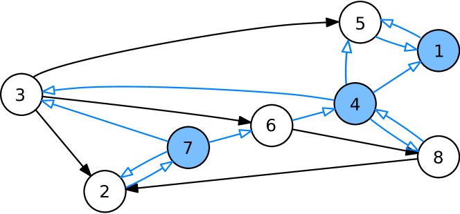
Figure 4: Connectivity graph $\Gamma$ of the example Hopfield network. Vertices that belong to the selected minimal FVS $\{1,4,7\}$ as well as their incoming and outgoing edges are highlighted in blue. There are no self-feedback loops because of the decay condition (III.2). Note, that $\Gamma$ possesses a second minimal FVS of same cardinality: $\{1,2,4\}$.

Remark IV.1.

In practice, when calculating $\mathbf{C}_{g}(t)$ according to Eq. 15 it is possible that upon initiation of control the Cauchy-Schwarz inequality Tripathi1999

$$\mathbf{C}_{KK}^{*}(t)\geq\mathbf{C}_{JK}^{*T}(t)\mathbf{C}_{JJ}^{-1}(t)\mathbf{C}_{JK}^{*}(t)$$ (18)

is not satisfied, leading to negative definite $\mathbf{C}_{g}$. This can occur because $\mathbf{C}_{KK}(t)$ and $\mathbf{C}_{JK}(t)$ are immediately forced to attain values on the target state, while the values of $\mathbf{C}_{JJ}$ still correspond to a distinct state. In other words, the moments system (Eqs. 17a and 17b) might be dragged to a point, where it is not possible to construct a physical counterpart given by Eq. 8 due to the constraints of probability laws. As a solution, we temporarily set $\mathbf{C}_{g}(t)\equiv 0$ in Eq. 10 at the time points, where $\mathbf{C}_{g}(t)$ would otherwise be invalid. For those time points $\mathbf{C}_{KK}(t)$ is no longer clamped to the target value $\mathbf{C}^{*}_{KK}(t)$. However, in this case, the MS still approximates the target state $(\boldsymbol{\mu}^{*}_{J}(t),\mathbf{C}^{*}_{JJ}(t))$, since the right-hand side of Eq. 17b only depends on $\mathbf{C}_{KK}$ via $\boldsymbol{\mu}_{J}(t)$, whose dynamics is dominated by $\mathbf{f}(t,\boldsymbol{\mu}_{J},\boldsymbol{\mu}_{K}^{*}(t))$ by weak noise assumption. As the system approaches the target state, $\mathbf{C}_{g}(t)$ becomes well-defined again (since, by construction, the target state has physical meaning). In Sections V and VI we employ this approach using Monte-Carlo simulations.

V Example 1: Hopfield network

We demonstrate the applicability of the theoretical results for general stochastic dynamical networks from Sections III and IV using an asymmetric Hopfield network Zheng2010. These networks possess a set of locally stable equilibrium states and a well-defined energy function (see, e.g., Zheng2010; Hopfield2007; Hopfield1984; Rojas1996). We consider a stochastic Hopfield network described by

$$\dot{\mathbf{x}}=-\mathbf{x}+\mathbf{G}\boldsymbol{\phi}(\mathbf{x})+\boldsymbol{\mu}_{\mathrm{ext}}+\sigma_{\mathrm{ext}}\boldsymbol{\eta}(t),$$ (19)

where $\mathbf{x}\in\mathbb{R}^{N}$ is the state vector, $\mathbf{G}$ the (asymmetric) coupling matrix, $\boldsymbol{\phi}:\mathbb{R}^{N}\to\mathbb{R}^{N}$ denotes an element-wise hyperbolic tangent function, i.e., $\boldsymbol{\phi}(\mathbf{x})=\left[\tanh(x_{1}),\dots,\tanh(x_{N})\right]^{T}$, $\boldsymbol{\mu}_{\mathrm{ext}}$ is the deterministic part of the external input, $\boldsymbol{\eta}(t)$ is a $N$-dimensional Gaussian white noise process, and $\sigma_{\mathrm{ext}}$ its (element-wise) standard deviation. Here, $N=8$ and $\mathbf{G}$ is given by the matrix

$$10^{-3}\cdot\begin{bmatrix}646&0&0&0&559&0&0&0\\ 0&462&0&0&0&0&-554&0\\ 0&-357&665&0&290&-373&0&0\\ 273&0&277&0&273&0&0&275\\ 559&0&0&0&646&0&0&0\\ 0&0&0&-558&0&0&0&-217\\ 0&-386&351&0&0&516&467&0\\ 0&299&0&643&0&0&0&405\end{bmatrix}$$

obtained using the algorithm described in Zheng2010, where the weakest edges were pruned to reduce the number of connections. The network graph (given by $\mathbf{G}$) with highlighted minimal FVS is shown in Fig. 4. Note that the decay condition (Assumption III.2) is fulfilled for all $N$ nodes since the diagonal elements of $\mathbf{G}$ are all $<1$. We further chose

$$\boldsymbol{\mu}_{\mathrm{ext}}=10^{-2}\cdot\begin{bmatrix}-32&-7&17&-36&32&16&-24&3\\ \end{bmatrix}^{T}$$

and $\sigma_{\mathrm{ext}}=0.01$ (larger values for $\sigma_{\mathrm{ext}}$ were also considered, see below).

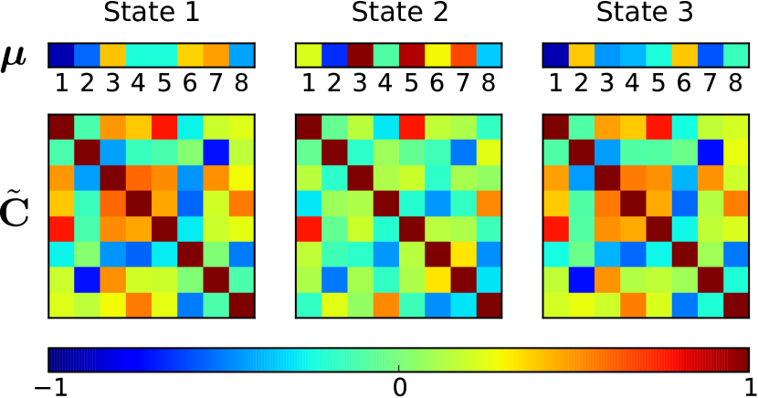
Figure 5: Metastable states of the example Hopfield network, given by Eq. 19 ($\sigma_{\mathrm{ext}}=0.01$). Values of mean vector $\boldsymbol{\mu}$ and correlation matrix $\tilde{\mathbf{C}}=(diag(\mathbf{C}))^{-\frac{1}{2}}\mathbf{C}(diag(\mathbf{C}))^{-\frac{1}{2}}$, with covariance matrix $\mathbf{C}$, for the three states. Note, that the three mean vectors are mutually distinct (approximately equidistant), the correlation matrices of state 1 and 3, however, are similar, but not the same.

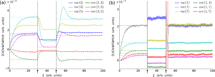
Figure 6: Switching states ($1\to 2\to 3$) of the Hopfield network ($\sigma_{\mathrm{ext}}=0.01$) by controlling the nodes of the FVS. Time tracks of (co)variances of (a) nodes $\{2,3,5\}$ and (b) the pinned nodes of the FVS $\{1,4,7\}$, obtained from Monte Carlo simulations (solid lines) and by solving the MS, Eqs. 17a and 17b (dashed lines). Dotted lines indicate the (co)variances values for states 1 ($t\leq 30$), 2 ($30<t\leq 50$), and 3 ($t>50$). Arrows at $t=30$ and $t=50$ mark the initiation of control. The shaded region starting at $t=50$ (right) indicates the period of time during which the noise intensity of the control signal is set to zero temporarily ($\mathbf{C}_{g}(t)=0$) to prevent violation of the Cauchy-Schwarz inequality (see Eq. 18). Note, that the Monte Carlo estimates of the pinned (co)variance values (i.e., those of $\mathbf{u}_{K}$) exhibit increased high (temporal) frequency because of the additive white Gaussian noise process of the control signal (cf. Eq. 10).

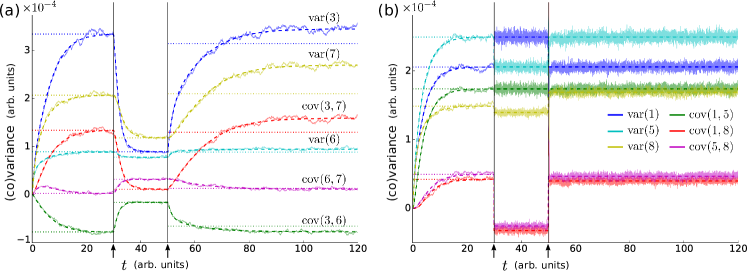
Figure 7: Switching states ($1\to 2\to 3$) of the Hopfield network ($\sigma_{\mathrm{ext}}=0.01$) by controlling the nodes $\{1,5,8\}$ (not a FVS). Time tracks of (co)variances of (a) nodes $\{3,6,7\}$ and (b) the pinned nodes $\{1,5,8\}$, obtained from Monte Carlo simulations (solid lines) and by solving the MS, Eqs. 17a and 17b (dashed lines). Dotted lines indicate the (co)variances values for states 1 ($t\leq 30$), 2 ($30<t\leq 50$), and 3 ($t>50$). Arrows mark the initiation of control. Note that switching $1\to 2$ succeeds, but the controller fails to steer the system to state 3.

With the parameter values specified above the network without noise, i.e., $\sigma_{\mathrm{ext}}=0$ in Eq. 19, possesses three stable fixed point attractors with roughly equal Euclidean distance between each two. This gives rise to three metastable states when noise is present ($\sigma_{\mathrm{ext}}>0$). That is, any solution trajectory of Eq. 19 will fluctuate around the corresponding fixed point of the noiseless system for a certain period of time but eventually will escape its attraction domain and approach another fixed point, thereby transitioning between metastable states. In other words, the solution of the Fokker-Planck equation that corresponds to the Langevin equation (19) will show a single peak close to one of the fixed points for a longer period of time – if the probability density is initialized around that fixed point – before the solution converges to the steady-state distribution that reveals additional peaks (equivalent to the Boltzmann distribution). The values of the mean vector $\boldsymbol{\mu}(t)$ and the covariance matrix $\mathbf{C}(t)$ that correspond to these three metastable states are visualized in Fig. 5.

All simulations were performed using Python with the libraries “SciPy” and “Theano” theano. The system of stochastic differential equations, Eq. 19, was solved using a stochastic 4th order Runge-Kutta method Kasdin1995 (integration step 0.01) and the corresponding MS given by a set of ordinary differential equations was solved using the LSODA integration method from “SciPy” (same integration step).

We used the controller described in Section IV to switch the state of the system (in terms of mean and covariance values) from state 1 to state 2 (at $t=30$), and subsequently to state 3 (at $t=50$), by pinning only the nodes of the FVS $K=\{1,4,7\}$. The system was initialized near the state 1 and evolved freely until the control method was applied. Immediately after that moment the states of the pinned nodes changed abruptly according to the control protocol. Specifically, given the target state $(\boldsymbol{\mu}^{*}(t),\mathbf{C}^{*}(t))$ we first solved the adapted MS, Eqs. 17a and 17b. Using that solution we next calculated the parameters $\boldsymbol{\mu}_{g}(t)$, $\mathbf{C}_{g}(t)$ and $\mathbf{W}(t)$ for the feedback control signal $\mathbf{u}_{K}^{*}(t,\mathbf{x}_{J}(t))$ according to Eqs. 10, 14, 15 and 16. Finally, we simulated the stochastic system 5000 times with the feedback controller $\mathbf{u}_{K}^{*}(t,\mathbf{x}_{J}(t))$ for different noise realizations to estimate the moments. The results of this procedure are shown in Figs. 6 and 7. The values of $\mathbf{C}(t)$ (subsets of $\mathbf{C}_{JJ}(t)$ and $\mathbf{C}_{KK}(t)$ shown in Figs. 6 and 7) and the values of $\boldsymbol{\mu}(t)$ (not shown) converge to the target values after a transient transition period. Note that the covariances between the clamped nodes ($\mathbf{C}_{KK}(t)$) may not follow the prescribed values immediately after pinning for that transient period, cf. Fig. 6 (b), as explained in Eq. 18. However, during the same period, the covariances between all other nodes ($\mathbf{C}_{JJ}(t)$) behave as predicted, cf. Fig. 6 (a).

Fig. 7 shows that choosing a subset of nodes that is not a FVS (nodes $\{1,5,8\}$) does not guarantee controllability of all metastable states. In particular, such controller fails to bring the system to state 3.

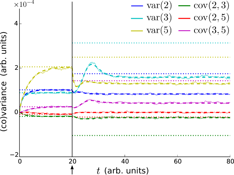
Figure 8: Switching states ($2\to 3$) of the Hopfield network ($\sigma_{\mathrm{ext}}=0.01$) by controlling the nodes of the FVS $K=\{1,4,7\}$ using an open-loop controller, Eq. 20. Time tracks of (co)variances of nodes $\{2,3,5\}$, obtained from Monte Carlo simulations (solid lines) and by solving the MS, Eqs. 17a and 17b (with $\boldsymbol{\mu}_{K}(t)\equiv\boldsymbol{\mu}_{K}^{*},\mathbf{C}_{KK}(t)\equiv\mathbf{C}_{KK}^{*},\mathbf{C}_{JK}(t)\equiv 0$, dashed lines). Dotted lines indicate the (co)variances values for states 2 ($t\leq 20$) and 3 ($t>20$). The arrow marks the initiation of control. Note, that the estimated (co)variance values (solid lines) follow the predictions from the MS solution (dashed lines), but do not converge to the target state.

Finally, we demonstrate that it does not suffice to control the moments $\boldsymbol{\mu}_{K}(t)$ and $\mathbf{C}_{KK}(t)$, i.e., the mean and covariance values among the nodes of the FVS, without controlling $\mathbf{C}_{JK}(t)$ as well. To show this we use the simplified control signal

$$\mathbf{u}_{K}^{*}(t)=\boldsymbol{\mu}_{K}^{*}(t)+\mathbf{C}_{KK}^{*\frac{1}{2}}(t)\boldsymbol{\eta}_{g}(t)$$ (20)

instead of $\mathbf{u}_{K}^{*}(t,\mathbf{x}_{J}(t))$ from Eq. 10. This leads to $\mathbf{C}_{JK}(t)=0$, since $\boldsymbol{\eta}_{J}(t)$ and $\boldsymbol{\eta}_{g}(t)$ are independent stochastic processes. As a consequence, the covariances $\mathbf{C}_{JJ}(t)$ are not guaranteed to converge to the target state (see Fig. 8).

We repeated the calculations for Figs. 6 and 7 using the same network system but with increased noise intensities ($\sigma=0.05,0.1$). For $\sigma=0.05$, the controller was able to switch the network state and hold it at the target, but the steady-state covariance values deviated slightly from their predicted values (not shown). This deterioration is caused by the (generally) decreased approximation quality of the method of moments for increased noise amplitudes. For $\sigma=0.1$ the MS becomes unstable (i.e., it looses its dissipativity) which precludes computation of the control signal. Therefore, in practice, the stability of the MS may be used to determine whether the noise is weak enough for successful application of the control method.

VI Example 2: brain network

To demonstrate the applicability of our theoretical results to larger systems we now consider a stochastic whole brain network model of 66 nodes which has been calibrated based on human diffusion imaging and functional magnetic resonance imaging data at rest, as described in Deco2013JN. Each node represents the pooled neuronal activation of a brain region and is governed by a nonlinear mean field model that consists of a stochastic scalar differential equation with additive noise (Eqs. (6)–(8) in Deco2013JN). The covariance matrices of the node variables indicate functional connectivity between brain regions. We use the same parameter values for the mean field model as in Deco2013JN, except for the kinetic parameter $\gamma$ which is changed to $\gamma=0.241\cdot 10^{-3}$ in order to meet the Assumption III.2. The network graph is given by a thresholded asymmetric structural connectivity matrix which was obtained using tractography based on diffusion (spectrum) imaging data and a partitioning of the brain into 66 regions, as described in Hagmann2008. The resulting weighted graph is visualized in Fig. 9 (a). Fig. 9 (b) shows the bifurcation diagram of the network states (in the absence of noise) as the global coupling parameter $G$ varies. For small values $G$ only one stable state exists, characterized by a low neuronal firing activity in all brain regions. As $G$ increases a first bifurcation emerges at a critical value, where multiple stable states of high activity appear and co-exist with the low activity state. As $G$ further increases a second bifurcation appears where the low activity state becomes unstable. This bifurcation diagram qualitatively resembles the one in Deco2013JN (Fig. 2).

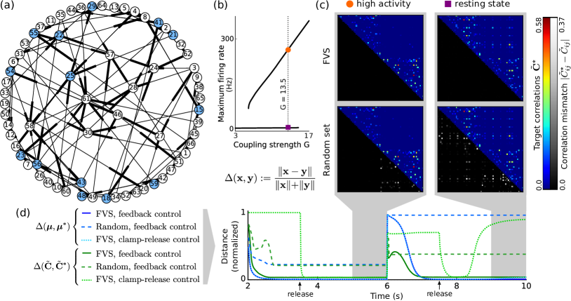
Figure 9: Brain network model. (a) Visualization of the weighted 66-node network graph. Nodes of the selected minimal FVS are highlighted in blue. Thick ends of the edges denote edge destination and strength. (b) Maximum firing rate of the network as a function of the global coupling strength $G$. Colored markers denote two different target states. (c) Correlation matrices at the target states (upper triangles) and their mismatch from the actual result of switching control (lower triangles). Rows correspond to two choices of nodes for the feedback control method: minimal FVS and a random set. Columns correspond to the target states indicated in (a). Correlation matrices are obtained by temporally averaging results of Monte-Carlo simulations ($2\cdot 10^{5}$ iterations) over 1 s after the system has converged. (d) Normalized distance $\Delta$ between the actual and the target states as a function of time, in terms of means and correlation matrices, for the feedback controller using FVS or random nodes, and for the clamp-release control scheme using FVS nodes. Note that diagonal elements are not considered when computing distance between correlation matrices (see Section VI). The system first evolves without control for 2 s. Then, the control method is applied to switch to the target high activity state and 4 s later it is adjusted to switch to the resting state. For clamp-release control, release occurs 1.5 s after each initiation.

We chose $G=13.5$, where the stochastic network possesses a metastable state of low activity (resting state) and a set of metastable states associated with high neuronal firing rates (“evoked” high activity states). We apply our feedback control method (Eq. 10) to switch the system to desired target states by directly interfering only with a minimal FVS $K$ of $14$ nodes, see Fig. 9 (c). In particular, the system was initialized close to the resting state, switched to a target high activity state after 2 s and back to the resting state 4 s later. For comparison we used, as an alternative, a “clamp-release” control strategy, where the FVS nodes were clamped deterministically to the target $\boldsymbol{\mu}^{*}$ for 1.5 s and then released, anticipating that the covariances would settle on the corresponding attractor in the moments space. We further used the feedback control method with three sets of randomly chosen nodes of the same size as the FVS (shown for one set). To assess the quality of control, we used the normalized distance $\Delta(\mathbf{x},\mathbf{y}):=\frac{\rVert\mathbf{x}-\mathbf{y}\lVert}{\rVert\mathbf{x}\lVert+\rVert\mathbf{y}\lVert}$ between the target state and the actual state of the system, where $\rVert\cdot\rVert$ is the Frobenius norm (Fig. 9 (d)). Note that when computing distances between correlation matrices we do not take into account elements on the diagonal, because $[\tilde{C}_{1}]_{ii}=[\tilde{C}_{2}]_{ii}=1$ for any two correlation matrices $\tilde{\mathbf{C}}_{1},\tilde{\mathbf{C}}_{2}$. Controlling the FVS nodes with the feedback controller successfully switched the system to the desired states after a relatively short period (i.e., both $\Delta(\boldsymbol{\mu}(t),\boldsymbol{\mu}^{*})$ and $\Delta(\tilde{\mathbf{C}}(t),\tilde{\mathbf{C}}^{*})$ vanish), while controlling a randomly chosen subset of nodes did not suffice. The clamp-release control scheme (applied to the FVS set) succeeded to bring the system to the high activity state with the appropriate correlation patterns, but failed to return it to the resting state ($\tilde{\mathbf{C}}(t)$ briefly approached $\tilde{\mathbf{C}}^{*}$ after the release of control but started to diverge in less than 1 s).

VII Discussion and Conclusion

In this contribution we have developed a control method that is capable of switching between metastable states – in terms of the first and second moments – of a large class of stochastic nonlinear dynamical networks by pinning only a subset of nodes. These nodes are identified based on information about the graph of the network. Our results can be applied in neuroscience, as demonstrated in Section VI, where the second moments of neuronal activities are often used to quantify functional connectivity. Because of their generality they may also be applied to a variety of problems in engineering or physics.

A central limitation of the presented approach is the assumption of weak noise (Assumption III.3), which is required for the applied method of moments and stability considerations in the proof of Eq. 6. Here, “weak” means that the probability density $p(x,t)$ of $x(t)$ (across noise realizations) should be concentrated around the expected value $\langle x\rangle(t)$.

The assumption of weak noise implies that the dynamics of the system are dominated by the deterministic part. It seems, therefore, tempting to steer the stochastic system to the desired state by pinning its set of SN deterministically to values on the corresponding target attractor of the noiseless system, and then “release” the control, to let the second moments settle corresponding to that attractor. Note, that releasing the control is required since deterministic pinning yields inappropriate correlation patterns, as explained in Section V. Releasing the control, however, can cause the system to rapidly transition to a different state (cf. Fig. 9 (d)) . We have demonstrated that the proposed feedback controller allows to hold desired metastable states for long periods, while maintaining the appropriate (desired) covariances.

Another limitation of the approach, is that the proposed feedback control signal, cf. Eq. 10, requires i) full observability of the network’s state to create non-zero covariance between the control signal and the network nodes, and ii) knowledge of the instantaneous moments to compute the proper feedback transformation matrix required to keep clamped covariances at their target values, cf. Eqs. 14 to 16. One way to obtain this data is to solve the moments system (Eqs. 17a and 17b), which requires knowledge of the system’s dynamics function $\mathbf{f}$, which might not be available. However, for systems with metastable fixed point states and weak $K\to J$ coupling (i.e., $||\nabla_{K}\mathbf{f}_{J}(t,\mathbf{x}_{J},\mathbf{x}_{K})||<\varepsilon$ for all $t,\mathbf{x}$ and small positive $\varepsilon$) this problem can be circumvented by using time invariant parameters $\boldsymbol{\mu}_{g},\mathbf{C}_{g}$ and $\mathbf{W}$, which are chosen such that conditions given by Eqs. 9a to 9c hold when $\boldsymbol{\mu}_{J}(t)\equiv\boldsymbol{\mu}_{J}^{*}$ and $\mathbf{C}_{JJ}(t)\equiv\mathbf{C}_{JJ}^{*}$:

$$\boldsymbol{\mu}_{g}=\boldsymbol{\mu}_{K}^{*}-\mathbf{C}_{JK}^{*T}\mathbf{C}^{*-1}_{JJ}\boldsymbol{\mu}_{J}^{*}$$ (21a)

$$\mathbf{C}_{g}=\mathbf{C}_{KK}^{*}-\mathbf{C}_{JK}^{*T}\mathbf{C}_{JJ}^{*-1}\mathbf{C}_{JK}^{*}$$ (21b)

$$\mathbf{W}=\mathbf{C}_{JJ}^{*-1}\mathbf{C}_{JK}^{*}$$ (21c)

The weak coupling ensures that the full derivative $\nabla_{J}\mathbf{f}_{J}(t,\mathbf{x}_{J},\mathbf{u}_{K}(\mathbf{x}_{J}))$ is dominated by $\nabla_{J}\mathbf{f}_{J}(\cdot,\mathbf{x}_{J},\cdot)$ which guarantees the existence of a global attractor in the controlled network. In this way, the control signal $\mathbf{u}_{K}(\mathbf{x}_{J})$ is based only on knowledge of the moments on the target state.

Finally, the FVS can be determined using a simple search procedure based on Definition III.2 (see Sec. 7.2 in Fiedler2013). For very large graphs, however, identification of the minimal FVS becomes computationally intractable, as the corresponding optimization problem is NP-complete Karp1972. Therefore, an interesting problem would be to find approximate minimal feedback vertex sets for large graphs at a reasonable computational cost.

VIII Acknowledgment

We thank Lutz Schimansky-Geier for helpful comments on the manuscript. This work was supported by DFG in the framework of collaborative research center SFB910.

Appendix Proof of Eq. 6

In order to prove Eq. 6 we first provide three useful propositions. Consider the deterministic system, Eq. 4, in terms of two coupled subsystems,

$$\dot{\mathbf{x}}_{K} =\mathbf{f}_{K}(t,\mathbf{x}_{K},\mathbf{x}_{J})$$ (22a)

$$\dot{\mathbf{x}}_{J} =\mathbf{f}_{J}(t,\mathbf{x}_{J},\mathbf{x}_{K}),$$ (22b)

cf. Eqs. 7a and 7b without the noise terms. We define $\mathbf{g}^{*}(t,\cdot):=\mathbf{f}_{J}(t,\cdot,\mathbf{x}^{*}_{K})$ for a particular solution $\mathbf{x}^{*}(t)$ of Eq. 4, such that

$$\dot{\mathbf{x}}_{J}=\mathbf{g}^{*}(t,\mathbf{x}_{J})$$ (23)

describes the dynamics of the state vector $\mathbf{x}_{J}$ where the time tracks of the nodes $K$ are prescribed to $\mathbf{x}^{*}_{K}(t)$.

In the following proposition we express the dynamics of the difference of any two solutions of Eq. 23 by a system of linear differential equations with time-varying coefficients and relate the asymptotic stability of that system to the controllability of the full system, Eqs. 22a and 22b, via the set of nodes $K$.

Proposition A.1.

Let the linear system

$$\dot{\mathbf{w}} =\mathbf{A}(t)\mathbf{w}$$ (24a)

$$\mathbf{A}(t) :=\int_{0}^{1}\nabla_{\mathbf{y}}\mathbf{g}^{*}(t,\mathbf{y}(t)+\nu[\tilde{\mathbf{y}}(t)-\mathbf{y}(t)])d\nu$$ (24b)

be globally asymptotically stable for any two solutions $\tilde{\mathbf{y}}(t)$, $\mathbf{y}(t)$ of

$$\dot{\mathbf{y}}=\mathbf{g}^{*}(t,\mathbf{y})$$ (25)

and any solution $\mathbf{x}^{*}(t)$ of Eq. 4. Then $K$ is a set of switching nodes (Definition III.1) of the system (4).

Proof.

Observe that

$$\frac{d}{dt}(\tilde{\mathbf{y}}-\mathbf{y})=\mathbf{g}^{*}(t,\tilde{\mathbf{y}})-\mathbf{g}^{*}(t,\mathbf{y})=\mathbf{A}(t)(\tilde{\mathbf{y}}-\mathbf{y}),$$ (26)

where we have used the Newton-Leibnitz formula for the equation on the right-hand side. Due to the stability assumption on Eq. 24a, the difference between any two solutions $\mathbf{y}$, $\tilde{\mathbf{y}}$ of Eq. 25 vanishes asymptotically as $t\to\infty$. Consequently, Eq. 25 possesses a unique globally attractive solution. By construction, for any solution $\mathbf{x}^{*}(t)$ of Eq. 4, $\mathbf{x}^{*}_{J}(t)$ is the globally attractive solution of Eq. 25. We obtain: $\mathbf{x}_{K}(t)=\mathbf{x}^{*}_{K}(t)\implies\mathbf{x}_{J}(t)\to\mathbf{x}^{*}_{J}(t)$ as $t\to\infty$. Thus, by Definition III.1, $K$ is a set of switching nodes. ∎

In the following, the notation $\mathbf{A}<\mathbf{B}<\mathbf{0}$ means that the matrices $\mathbf{A}$, $\mathbf{B}$ and $\mathbf{A}-\mathbf{B}$ are (strictly) negative definite, i.e. $\mathbf{x}^{T}\mathbf{A}\mathbf{x}<0,\forall\mathbf{x}\neq\mathbf{0}$.

Proposition A.2.

Let $\mathbf{A}(t):\mathbb{R}\to\mathbb{R}^{k\times k},k=\sum_{i=1}^{N}m_{i}$ be a continuous and uniformly bounded block-triangular matrix function, with $N$ blocks $\mathbf{A}_{i}(t)$, $i\in\{1,\dots,N\}$ on the main diagonal, and let each block $\mathbf{A}_{i}(t)$ be negative definite and bounded from above, i.e., $\mathbf{A}_{i}(t)<\bar{\mathbf{A}}_{i}<\mathbf{0}$ for all $t\geq 0$. Then, for any continuous and uniformly bounded matrix function $\mathbf{B}(t)$, there exists an $\varepsilon>0$, such that the (trivial) solution $\mathbf{z}(t)\equiv\mathbf{0}$ of the system

$$\dot{\mathbf{z}}=[\mathbf{A}(t)+\varepsilon\mathbf{B}(t)]\mathbf{z}$$ (27)

is globally asymptotically stable.

Proof.

We first transform the unperturbed system

$$\dot{\mathbf{z}}=\mathbf{A}(t)\mathbf{z},$$ (28)

to an equivalent system $\dot{\mathbf{y}}=\tilde{\mathbf{A}}(t)\mathbf{y}$ with triangular matrix $\tilde{\mathbf{A}}(t)$. The fundamental solution matrix $\mathbf{Z}(t)$ of Eq. 28 can be uniquely QL-factorized, $\mathbf{Z}(t)=\mathbf{Q}(t)\mathbf{L}(t)$, where $\mathbf{Q}(t)$ is orthonormal and $\mathbf{L}(t)$ is a lower triangular matrix. Moreover, because $\mathbf{Z}(t)$ is lower block-triangular, the matrix $\mathbf{Q}(t)$ is block-diagonal with blocks $\mathbf{Z}_{i}(t)=\mathbf{Q}_{i}(t)\mathbf{L}_{i}(t)$. Using the change of basis $\mathbf{z}=\mathbf{Q}(t)\mathbf{y}$ we obtain (time dependence of $\mathbf{A}$ and $\mathbf{Q}$ is implied):

$$\dot{\mathbf{y}}=(\mathbf{Q}^{T}\mathbf{A}\mathbf{Q}-\mathbf{Q}^{T}\dot{\mathbf{Q}})\mathbf{y}=:\tilde{\mathbf{A}}(t)\mathbf{y},$$ (29)

where $\tilde{\mathbf{A}}(t)$ is continuous, uniformly bounded and lower-triangular. Note that since the diagonal blocks $\mathbf{A}_{i}(t)$ of $\mathbf{A}(t)$ are negative definite for all $t$, and $\mathbf{Q}(t)$ is block-diagonal with blocks $\mathbf{Q}_{i}(t)$, all diagonal entries of $\mathbf{Q}^{T}\mathbf{A}\mathbf{Q}$ are negative and bounded from above, i.e., for each diagonal block $\mathbf{D}_{i}:=\mathbf{Q}_{i}^{T}\mathbf{A}_{i}\mathbf{Q}_{i}$, we have $[D_{i}]_{jj}=\mathbf{q}_{j}^{T}(t)\mathbf{A}_{i}(t)\mathbf{q}_{j}(t)<\bar{a}<0$, $\forall t$, where $i\in\{1,\dots,N\}$, $j\in\{1,\dots,m_{i}\}$ and $\mathbf{q}_{j}(t)$ is the $j$-th column of $\mathbf{Q}_{i}(t)$. Moreover, the matrix $\mathbf{Q}^{T}\dot{\mathbf{Q}}$ is skew-symmetric and hence has zeros on the main diagonal (since $\mathbf{Q}^{T}\mathbf{Q}=\mathbf{I}$ and thus $d(\mathbf{Q}^{T}\mathbf{Q})/dt=\dot{\mathbf{Q}}^{T}\mathbf{Q}+\mathbf{Q}^{T}\dot{\mathbf{Q}}=\mathbf{0}$). It follows that the diagonal entries $\tilde{\mathbf{A}}(t)$ are continuous, negative and bounded from above.

Using the same change of basis $\mathbf{z}=\mathbf{Q}(t)\mathbf{y}$ for Eq. 27, we obtain

$$\dot{\mathbf{y}}=[\tilde{\mathbf{A}}(t)+\varepsilon\tilde{\mathbf{B}}(t)]\mathbf{y},$$ (30)

with $\tilde{\mathbf{B}}:=\mathbf{Q}^{T}\mathbf{B}\mathbf{Q}$. According to Theorem 1.1 in Dai2006, if the condition

$$\chi:=\limsup_{s\to+\infty}\frac{1}{T_{s}}\sum_{s^{\prime}=0}^{s-1}\max_{1\leq k\leq N}\left\{\int_{T_{s^{\prime}}}^{T_{s^{\prime}+1}}\tilde{A}_{kk}(t)dt\right\}<0$$ (31)

is fulfilled, then for any given $\delta>0$ there exists an upper bound $\gamma$ on the norm of the perturbation $\varepsilon\tilde{\mathbf{B}}(t)$, i.e., $\varepsilon||\tilde{\mathbf{B}}(t)||<\gamma$ such that the maximum Lyapunov exponent for the trivial solution of the system (30) is bounded from above by $\chi+\delta$. Given that the diagonal elements of $\tilde{\mathbf{A}}(t)$ are negative and bounded from above (for all $t$), the condition (31) holds for any partitioning $\{T_{s}\}_{0}^{\infty}$, and $\chi\leq\bar{a}$. Therefore, there exists a sufficiently small $\varepsilon>0$ such that the system Eq. 30 is asymptotically and exponentially stable.

Finally, observe that by Theorem 7.11 from meiss2007, the characteristic exponents of the systems (27) and (30) are identical. ∎

Next, we provide a generalization of the Kronecker sum operation $\oplus$ for partitioned matrices.

Proposition A.3.

Let $\mathbf{A},\mathbf{B}\in\mathbb{C}^{k\times k},k=\sum_{i=1}^{N}m_{i}$ be two partitioned lower block-triangular matrices with $N$ blocks on the main diagonal. Each diagonal block $\mathbf{A}_{i}$ and $\mathbf{B}_{i}$ is a square $m_{i}\times m_{i}$ matrix. All the elements above the diagonal blocks are zero. Then there exist a block diagonal permutation matrix $\mathbf{P}\in\{0,1\}^{k^{2}\times k^{2}}$, such that the matrix

$$\mathbf{S}:=\mathbf{P}(\mathbf{A}\oplus\mathbf{B})\mathbf{P}$$ (32)

is again block-triangular, with $N^{2}$ blocks on the main diagonal, given by

$$\mathbf{S}_{i,j}:=\mathbf{S}_{i(N-1)+j}=\mathbf{B}_{j}\oplus\mathbf{A}_{i},$$ (33)

where $i,j\in\{1,\dots,N\}$.

Proof.

By definition, the matrix $\mathbf{A}\oplus\mathbf{B}$ is given by

$$\mathbf{S}^{\prime}:=\mathbf{A}\oplus\mathbf{B}=\mathbf{A}\otimes\mathbf{I}+\mathbf{I}\otimes\mathbf{B},$$ (34)

where $\otimes$ is the Kronecker product and $\mathbf{I}$ is the $k\times k$ identity matrix. $\mathbf{S}^{\prime}$ has $N$ blocks $\mathbf{S}^{\prime}_{i}$, $i\in\{1,\dots,N\}$, of dimension $m_{i}k\times m_{i}k$ on the main diagonal, $\mathbf{S}^{\prime}_{i}=\mathbf{A}_{i}\otimes\mathbf{I}+\mathbf{I}_{i}\otimes\mathbf{B}$, where $\mathbf{I}_{i}$ is the $m_{i}\times m_{i}$ identity matrix. We next design a block-wise permutation matrix $\mathbf{P}$ such that each block $\mathbf{S}^{\prime}_{i}$ itself has a block structure. To that end, we define a block-diagonal matrix $\mathbf{P}$ with the same block partitioning of the main diagonal as the matrix $\mathbf{S}^{\prime}$. Let each block $\mathbf{P}_{i}$ of $\mathbf{P}$ be a commutation matrix, such that $\mathbf{P}_{i}(\mathbf{D}\otimes\mathbf{E})\mathbf{P}_{i}=\mathbf{E}\otimes\mathbf{D}$ for any two matrices $\mathbf{D}$ and $\mathbf{E}$ of dimensions $m_{i}\times m_{i}$ and $k\times k$, respectively. Then the blocks $\mathbf{S}_{i}$ on the main diagonal of $\mathbf{S}:=\mathbf{P}\mathbf{S}^{\prime}\mathbf{P}$ are given by

$$\mathbf{S}_{i}=\mathbf{P}_{i}\mathbf{S}^{\prime}_{i}\mathbf{P}_{i}=\mathbf{I}\otimes\mathbf{A}_{i}+\mathbf{B}\otimes\mathbf{I}_{i}.$$ (35)

Note that each block $\mathbf{S}_{i}$ is block-triangular, and the $j$-th nested block $\mathbf{S}_{i,j}$ on the main diagonal of $\mathbf{S}_{i}$ reads

$$\mathbf{S}_{i,j}=\mathbf{I}_{j}\otimes\mathbf{A}_{i}+\mathbf{B}_{j}\otimes\mathbf{I}_{i}=\mathbf{B}_{j}\oplus\mathbf{A}_{i},$$ (36)

for $i,j\in\{1,\dots,N\}$. Hence, $\mathbf{P}(\mathbf{A}\oplus\mathbf{B})\mathbf{P}$ is a block-triangular matrix with $N^{2}$ blocks as given by Eq. 36. ∎

Proof of Eq. 6.

Consider the network system, Eq. 2, as represented by the two coupled subsystems, Eqs. 7a and 7b. Let the set $J$ be topologically sorted according to the directed acyclic subgraph of the nodes in the set $I\setminus K$, such that node $J[1]$ has incoming edges only from the nodes in $K$, $J[2]$ – only from the nodes in $K\cup J[1]$, etc. With this ordering of the nodes represented by the state vector $\mathbf{x}_{J}$ (and the components $\mathbf{f}_{J}$, $\mathbf{M}_{J}$, $\boldsymbol{\eta}_{J}$ in Eq. 7b ordered correspondingly) the Jacobian matrix $\nabla_{J}\mathbf{f}_{J}(t,\mathbf{x}_{J},\mathbf{x}_{K})$ is a lower block-triangular matrix, and each block on the main diagonal is strictly negative definite for all $t$ and bounded $\mathbf{x}$ due to the decay condition (Assumption III.2). Note, that for multivariate nodes ($m_{i}>1$), the ordering affects $\mathbf{x}_{J}$ “block-wise”: $\mathbf{x}_{J}=[\mathbf{x}_{J[1]}^{T},\mathbf{x}_{J[2]}^{T},\dots,\mathbf{x}_{J[N-|K|]}^{T}]^{T}$.

Let $\boldsymbol{\mu}_{J}(t):=\langle\mathbf{x}_{J}\rangle(t)$ and $\mathbf{C}_{JK}(t):=cov(\mathbf{x}_{J},\mathbf{x}_{K})(t)=\langle\mathbf{x}_{J}\mathbf{x}_{K}^{T}\rangle(t)-\boldsymbol{\mu}_{J}(t)\boldsymbol{\mu}_{K}^{T}(t)$ as used in Section IV. That is, the $m_{i}\times m_{j}$ submatrix $\mathbf{C}_{ij}(t)$ of $\mathbf{C}_{JJ}(t)$ is the covariance matrix between $\mathbf{x}_{J[i]}(t)$ and $\mathbf{x}_{J[j]}(t)$. $K^{*}:=\{\boldsymbol{\mu}_{K},\mathbf{C}_{KK},\mathbf{C}_{JK},\mathbf{C}_{KJ}\}$ then denotes the set of switching node candidates, cf. Eq. 6. Using Proposition A.1 we can now prove Eq. 6 by showing the stability of the solution of the subsystem, Eqs. 17a and 17b, of the MS, Eqs. 3a and 3b, where the moments $\boldsymbol{\mu}_{K}(t)=\boldsymbol{\mu}_{K}^{*}(t)$, $\mathbf{C}_{KK}(t)=\mathbf{C}_{KK}^{*}(t)$, $\mathbf{C}_{JK}(t)=\mathbf{C}_{KJ}^{T}(t)=\mathbf{C}_{JK}^{*}(t)$ are pinned.

It is convenient to express Eqs. 17a and 17b in compact form as

$$\dot{\boldsymbol{\gamma}}_{J}=\mathbf{h}_{J}(t,\boldsymbol{\gamma}_{J},\boldsymbol{\gamma}_{K}),$$ (37)

where $\boldsymbol{\gamma}_{J}=[\mathbf{C}_{JJ[1]}^{T},\dots,\mathbf{C}_{JJ[N-|K|]}^{T},\boldsymbol{\mu}_{J}^{T}]^{T}\in\mathbb{R}^{k_{J}^{2}+k_{J}}$, $k_{J}:=\sum_{i\in J}m_{i}$ contains $\boldsymbol{\mu}_{J}$ and the columns of $\mathbf{C}_{JJ}$. Considering the Jacobian matrix $\mathbf{U}=\mathbf{U}(t,\boldsymbol{\gamma}_{J},\boldsymbol{\gamma}_{K}):=\nabla_{J}\mathbf{h}_{J}(t,\boldsymbol{\gamma}_{J},\boldsymbol{\gamma}_{K})$ the following block structure can be identified:

$$\begin{array}{ccc}\hfill 𝐔& =[c.cc.c\nabla {}_J𝐟{}_J\oplus \nabla {}_J𝐟\hfill & \hfill 𝐁{}_1\\ \multicolumn{2}{c}{\nabla {}_J𝐟{}_J+𝐁{}_2]}\\ & =[\hfill & \hfill 0\\ \multicolumn{2}{c}{𝐀]+[}& \hfill 𝐁{}_1\\ \multicolumn{2}{c}{𝐁{}_2]=:𝐔{}_L+𝐁,}\end{array}where\text{A}\text{ = }\text{A}\text{(t,}\text{γ}\text{\_J, }\text{γ}\text{\_K):=∇\_J}\text{f}\text{\_J(t, }\text{μ}\text{\_J,}\text{μ}\text{\_K)}and\text{B}\text{= }\text{B}\text{(t,}\text{γ}\text{\_J, }\text{γ}\text{\_K) = }\text{B}\text{(t, }\text{μ}\text{, }\text{C}\text{)}isaboundedmatrixfunctionthatislinearwithrespectto\text{C}\text{(t)}andinvolvessecondandthirdderivativesof\text{f}\text{\_J}.Note,that\text{U}\text{\_L = }\text{U}\text{\_L(t,}\text{γ}\text{\_J, }\text{γ}\text{\_K)}isalowerblock-triangularmatrix.The\text{k\_J×k\_J}lower-rightblockof\text{U}\text{\_L},i.e.,\text{A},isalowerblock-triangularmatrixwithnegativedefiniteblocks\text{A}\text{\_i:=∇\_J[i]}\text{f}\text{\_J[i]}onthemaindiagonal,aswasnotedabove.Consideringthe\text{k\_J^2×k\_J^2}upper-leftblockof\text{U}\text{\_L}weknow,by\text{<a href="\#A1.Thmprop3" title="Proposition A.3. ‣ Appendix Proof of Eq. 6 ‣ Controlling statistical moments of stochastic dynamical networks" class="ltx\_ref ltx\_font\_italic"><span class="ltx\_text ltx\_ref\_tag">Proposition</span> <span class="ltx\_text ltx\_ref\_tag">A.3</span></a>},thatthereexistsapermutationmatrix\text{P}suchthatthematrix\text{P}\text{(}\text{A}\text{⊕}\text{A}\text{)}\text{P}islowerblock-triangularwith\text{N^2}blocks,eachgivenby\text{A}\text{\_j ⊕}\text{A}\text{\_i}.Furthermore,eachoftheseblocksisnegativedefinite,whichcanbeseenbyinspectingthehermitianparts\text{H}\text{\_i,j := (}\text{A}\text{\_j ⊕}\text{A}\text{\_i) + (}\text{A}\text{\_j ⊕}\text{A}\text{\_i)^T},sinceamatrixisnegativedefiniteiffitshermitianpartisnegativedefinite:\text{(39)Equation 39Eq.EquationEqs.Equations39Hi,j=(Aj⊕Ai)+(Aj⊕Ai)T=Aj⊗Ii+AjT⊗Ii+Ij⊗Ai+Ij⊗AiT=(Aj+AjT)⊗Ii+Ij⊗(Ai+AiT).}So,\text{H}\text{\_i,j}isasumoftworealsymmetricmatrices,bothofwhichhaveonlynegativeeigenvalues,hence\text{H}\text{\_i,j}andconsequently\text{A}\text{\_j ⊕}\text{A}\text{\_i}arenegativedefinite.Asaresult,usingasuitablepermutationmatrix\text{V},theJacobian\text{U}\text{\_L’(t,}\text{γ}\text{\_J, }\text{γ}\text{\_K):=}\text{VU}\text{\_L(t,}\text{γ}\text{\_J, }\text{γ}\text{\_K)}\text{V}isalowerblock-triangularmatrixwith\text{N+N^2}negativedefiniteblocksforall\text{t}andbounded\text{γ}\text{\_J},\text{γ}\text{\_K}.Moreover,theelement-wiseintegratedmatrix\text{(40)Equation 40Eq.EquationEqs.Equations40^UL′(t):=∫01UL′(t,ξ(t,ν),γK(t))dν}preservestheaforementionedpropertiesof\text{U}\text{\_L’}foranybounded\text{ξ}\text{(t, }\text{ν}\text{) ∈}\text{R}\text{^k\_J + k\_J^2}and\text{γ}\text{\_K(t)}.By\text{<a href="\#A1.Thmprop1" title="Proposition A.1. ‣ Appendix Proof of Eq. 6 ‣ Controlling statistical moments of stochastic dynamical networks" class="ltx\_ref ltx\_font\_italic"><span class="ltx\_text ltx\_ref\_tag">Proposition</span> <span class="ltx\_text ltx\_ref\_tag">A.1</span></a>},wehavethat\text{K^*}isindeedasetofSNsof\text{<a href="\#S2.E3.1" title="In Equation 3 ‣ II Stochastic network model and the moments system ‣ Controlling statistical moments of stochastic dynamical networks" class="ltx\_ref ltx\_font\_italic"><span class="ltx\_text ltx\_ref\_tag">Eqs.</span> <span class="ltx\_text ltx\_ref\_tag">3a</span></a>}and\text{<a href="\#S2.E3.2" title="Equation 3b ‣ Equation 3 ‣ II Stochastic network model and the moments system ‣ Controlling statistical moments of stochastic dynamical networks" class="ltx\_ref ltx\_font\_italic"><span class="ltx\_text ltx\_ref\_tag">3b</span></a>},ifthematrix\widehat{\text{U}}\text{’(t) := ∫}\text{VUV}\text{ =: }\widehat{\text{U}}\text{\_L’(t) + }\widehat{\text{B}}\text{’(t)}yieldsagloballystablelinearnonautonomoussystem\text{(41)Equation 41Eq.EquationEqs.Equations41˙w=^U′(t)w.}Bytheassumptionofweaknoise(\text{<a href="\#S3.Thmassumption3" title="Assumption III.3. ‣ III Identifying network nodes for control ‣ Controlling statistical moments of stochastic dynamical networks" class="ltx\_ref ltx\_font\_italic"><span class="ltx\_text ltx\_ref\_tag">Assumption</span> <span class="ltx\_text ltx\_ref\_tag">III.3</span></a>})\text{sup\_t∈}\text{R}\text{^+——}\text{C}\text{(t)—— ¡ }\text{ς}withsmall\text{ς}\text{¿0}.Becausetheperturbationmatrix\text{B}islinearin\text{C}\text{(t)},thenormof\widehat{\text{B}}\text{’(t)}multiplicativelydependson\text{ς},andthereforecanbearbitrarysmall,assumingboundedsecondandthirdderivativesof\text{f}\text{\_J}.Hence,by\text{<a href="\#A1.Thmprop2" title="Proposition A.2. ‣ Appendix Proof of Eq. 6 ‣ Controlling statistical moments of stochastic dynamical networks" class="ltx\_ref ltx\_font\_italic"><span class="ltx\_text ltx\_ref\_tag">Proposition</span> <span class="ltx\_text ltx\_ref\_tag">A.2</span></a>},thereexistsasufficientlysmall\text{ς},suchthatthesolutionof\text{<a href="\#A1.E41a" title="In 41 ‣ Proof of Eq. 6. ‣ Appendix Proof of Eq. 6 ‣ Controlling statistical moments of stochastic dynamical networks" class="ltx\_ref ltx\_font\_italic"><span class="ltx\_text ltx\_ref\_tag">Eq.</span> <span class="ltx\_text ltx\_ref\_tag">41</span></a>}isgloballyasymptoticallystable.\mathit{∎}\text{References12003Newman}$$ (41)