COMPUTATION OF GENERALIZED MATRIX FUNCTIONS

Abstract

We develop numerical algorithms for the efficient evaluation of quantities associated with generalized matrix functions [J. B. Hawkins and A. Ben-Israel, Linear and Multilinear Algebra, 1(2), 1973, pp. 163–171]. Our algorithms are based on Gaussian quadrature and Golub–Kahan bidiagonalization. Block variants are also investigated. Numerical experiments are performed to illustrate the effectiveness and efficiency of our techniques in computing generalized matrix functions arising in the analysis of networks.

1 Introduction

Generalized matrix functions were first introduced by Hawkins and Ben-Israel in [15] in order to extend the notion of a matrix function to rectangular matrices. Essentially, the definition is based on replacing the spectral decomposition of $A$ (or the Jordan canonical form, if $A$ is not diagonalizable) with the singular value decomposition, and evaluating the function at the singular values of $A$, if defined. While it is likely that this definition was inspired by the analogy between the inverse and the Moore–Penrose generalized inverse, which is well established in numerical linear algebra, [15] is a purely theoretical paper and does not mention any potential applications or computational aspects. The paper appears to have gone largely unnoticed, despite increasing interest in matrix functions in the numerical linear algebra community over the past several years; for instance, it is not cited in the important monograph by Higham [16]. While it is likely that the perceived scarcity of applications is to blame (at least in part) for this lack of attention, it turns out that generalized matrix functions do have interesting applications and have actually occurred in the literature without being recognized as such; see section 4 for some examples.

In this paper we revisit the topic of generalized matrix functions, with an emphasis on numerical aspects. After reviewing the necessary background and definitions, we consider a few situations naturally leading to generalized matrix functions. Moving on to numerical considerations, we develop several computational approaches based on variants of Golub–Kahan bidiagonalization to compute or estimate bilinear forms involving generalized matrix functions, including entries of the generalized matrix function itself and the action of a generalized matrix function on a vector. We further consider block variants of Golub–Kahan bidiagonalization which can be used to evaluate matrix-valued expressions involving generalized matrix functions. Numerical experiments are used to illustrate the performance of the proposed techniques on problems arising in the analysis of directed networks.

2 Background

In this section we review a few basic concepts from linear algebra that will be used throughout the paper, mostly to set our notation, and recall the notion of generalized matrix function.

Let $A\in{{\mathbb{C}}^{m\times n}}$ and let $r$ be the rank of $A$. We can factor the matrix $A$ as $A=U\Sigma V^{*}$ using a singular value decomposition (SVD). The matrix $\Sigma\in{{\mathbb{R}}^{m\times n}}$ is diagonal and its entries $\Sigma_{ii}=\sigma_{i}$ are ordered as $\sigma_{1}\geq\sigma_{2}\geq\cdots\geq\sigma_{r}>\sigma_{r+1}=\cdots=\sigma_{q}=0$, where $q=\min\{m,n\}$. The $r$ positive $\sigma_{i}$ are the singular values of $A$. The matrices $U=[{\bf u}_{1},{\bf u}_{2},\ldots,{\bf u}_{m}]\in{\mathbb{C}}^{m\times m}$ and $V=[{\bf v}_{1},{\bf v}_{2},\ldots,{\bf v}_{n}]\in{\mathbb{C}}^{n\times n}$ are unitary and contain the left and right singular vectors of $A$, respectively. It is well known that the matrix $\Sigma$ is uniquely determined, while $U$ and $V$ are not. If $A$ is real, then $U$ and $V$ can be chosen to be real. From the singular value decomposition of a matrix $A$ it follows that $AA^{*}=U\Sigma\Sigma^{T}U^{*}$ and $A^{*}A=V\Sigma^{T}\Sigma V^{*}$. Thus, the singular values of a matrix $A$ are the square roots of the positive eigenvalues of the matrix $AA^{*}$ or $A^{*}A$. Moreover, the left singular vectors of $A$ are the eigenvectors of the matrix $AA^{*}$, while the right singular vectors are the eigenvectors of the matrix $A^{*}A$. The singular values of a matrix also arise (together with their opposites) as the eigenvalues of the Hermitian matrix

(1) $$\mathscr{A}=\left(\begin{array}[]{cc}0&A\\ A^{*}&0\end{array}\right).$$

This can be easily seen for the case $m=n$; indeed, under this hypothesis, the spectral factorization of $\mathscr{A}$ is given by [17]:

$$\mathscr{A}=\frac{1}{2}\left(\begin{array}[]{cc}U&-U\\ V&V\end{array}\right)\left(\begin{array}[]{cc}\Sigma&0\\ 0&-\Sigma\end{array}\right)\left(\begin{array}[]{cc}U&-U\\ V&V\end{array}\right)^{*}.$$

Consider now the matrices $U_{r}\in{\mathbb{C}}^{m\times r}$ and $V_{r}\in{\mathbb{C}}^{n\times r}$ which contain the first $r$ columns of the matrices $U$ and $V$, respectively, and let $\Sigma_{r}\in{\mathbb{R}}^{r\times r}$ be the $r\times r$ leading block of $\Sigma$. Then a compact SVD (CSVD) of the matrix $A$ is

$$A=U_{r}\Sigma_{r}V^{*}_{r}=\sum_{i=1}^{r}\sigma_{i}{\bf u}_{i}{\bf v}_{i}^{*}.$$

2.1 Matrix functions

There are several equivalent ways to define $f(A)$ when $A\in{\mathbb{C}}^{n\times n}$ is a square matrix. We recall here the definition based on the Jordan canonical form. For a comprehensive study of matrix functions, we refer to [16].

Let $\{\lambda_{1},\lambda_{2},\ldots,\lambda_{s}\}$ be the set of distinct eigenvalues of $A$ and let $n_{i}$ denote the index of the $i$th eigenvalue, i.e., the size of the largest Jordan block associated with $\lambda_{i}$. Recall that a function $f$ is said to be defined on the spectrum of $A$ if the values $f^{(j)}(\lambda_{i})$ exist for all $j=0,\ldots,n_{i}-1$ and for all $i=1,\ldots,s$, where $f^{(j)}$ is the $j$th derivative of the function and $f^{(0)}=f$.

Definition 1.

[16, Definition 1.2] Let $f$ be defined on the spectrum of $A\in{\mathbb{C}}^{n\times n}$ and let $Z^{-1}AZ=J=\mathop{\operator@font diag}\nolimits(J_{1},J_{2},\ldots,J_{p})$ be the Jordan canonical form of the matrix, where

$$J_{k}=J_{k}(\lambda_{k})=\left(\begin{array}[]{cccc}\lambda_{k}&1&&\\ &\lambda_{k}&\ddots&\\ &&\ddots&1\\ &&&\lambda_{k}\end{array}\right)\in{\mathbb{C}}^{m_{k}\times m_{k}},$$

$\sum_{k=1}^{p}m_{k}=n$, and $Z$ is nonsingular. Then

$$f(A):=Zf(J)Z^{-1}=Z\mathop{\operator@font diag}\nolimits(f(J_{1}),f(J_{2}),\ldots,f(J_{p}))Z^{-1},$$

where

$$f(J_{k}):=\left(\begin{array}[]{cccc}f(\lambda_{k})&f^{\prime}(\lambda_{k})&\cdots&\frac{f^{(m_{k}-1)}(\lambda_{k})}{(m_{k}-1)!}\\ &f(\lambda_{k})&\ddots&\vdots\\ &&\ddots&f^{\prime}(\lambda_{k})\\ &&&f(\lambda_{k})\end{array}\right),$$

If the matrix $A$ is diagonalizable, then the Jordan canonical form reduces to the spectral decomposition: $A=ZDZ^{-1}$ with $D=\mathop{\operator@font diag}\nolimits(\lambda_{1},\lambda_{2},\ldots,\lambda_{n})$. In such case, $f(A)=Z\mathop{\operator@font diag}\nolimits(f(\lambda_{1}),f(\lambda_{2}),\ldots,f(\lambda_{n}))Z^{-1}$.

If the function $f$ has a Taylor series expansion, we can use it to describe the associated matrix function, provided that the eigenvalues of the matrix $A$ satisfy certain requirements.

Theorem 2.

[16, Theorem 4.7] Let $A\in{\mathbb{C}}^{n\times n}$ and suppose that $f$ can be expressed as

$$f(z)=\sum_{k=0}^{\infty}a_{k}(z-z_{0})^{k}$$

with radius of convergence $R$. Then $f(A)$ is defined and is given by

$$f(A)=\sum_{k=0}^{\infty}a_{k}(A-z_{0}I)^{k}$$

if and only if each of the distinct eigenvalues of $A$ $\{\lambda_{1},\lambda_{2},\ldots,\lambda_{s}\}$ satisfies one of the following:

• $|\lambda_{i}-z_{0}|<R$;

• $|\lambda_{i}-z_{0}|=R$ and the series for $f^{(n_{i}-1)}(\lambda)$ is convergent at the point $\lambda=\lambda_{i}$, $i=1,2,\ldots,s$.

2.2 Generalized matrix functions

In [15] the authors considered the problem of defining functions of rectangular matrices. Their definition relies on the following generalization of the SVD.

Theorem 3.

Let $A\in{\mathbb{C}}^{m\times n}$ be a matrix of rank $r$ and let $\{c_{i}:i=1,2,\ldots,r\}$ be any complex numbers satisfying

$$|c_{i}|^{2}=\sigma_{i}^{2}=\lambda_{i}(AA^{*}),$$

where $\lambda_{1}(AA^{*})\geq\lambda_{2}(AA^{*})\geq\cdots\geq\lambda_{r}(AA^{*})>0$ are the positive eigenvalues of $AA^{*}$. Then there exist two unitary matrices ${\pcal X}\in{\mathbb{C}}^{m\times m}$ and ${\pcal Y}\in{\mathbb{C}}^{n\times n}$ such that ${\pcal D}={\pcal X}^{*}A{\pcal Y}\in{{\mathbb{C}}^{m\times n}}$ has entries:

$$d_{ij}=\left\{\begin{array}[]{ll}c_{i}&{\rm if}\ 1\leq i=j\leq r\,,\\ 0&{\rm otherwise.}\end{array}\right.$$

From this theorem it follows that, once the non-zero entries of $\pcal{D}$ are fixed, $A$ can be written as

(2) $$A={\pcal X}{\pcal D}{\pcal Y}^{*}={\pcal X}_{r}{\pcal D}_{r}{\pcal Y}_{r}^{*},$$

where ${\pcal D}_{r}$ is the leading $r\times r$ block of ${\pcal D}$ and the matrices ${\pcal X}_{r}\in{\mathbb{C}}^{m\times r}$ and ${\pcal Y}_{r}\in{\mathbb{C}}^{n\times r}$ consist of the first $r$ columns of the matrices ${\pcal X}$ and ${\pcal Y}$, respectively.

In this paper we do not make use of the extra degrees of freedom provided from this (slightly) more general SVD of $A$, and we assume that $c_{i}=\sigma_{i}$ for all $i=1,2,\ldots,r$. This assumption ensures that the decompositions in (2) coincide with the SVD and CSVD of the matrix $A$, respectively. In particular, ${\pcal D}=\Sigma$, ${\pcal X}=U$, and ${\pcal Y}=V$. All the definitions and results presented in the remaining of this section and in the next one can be extended to the case when the coefficients $\{c_{i}:i=1,2,\ldots,r\}$ do not necessarily coincide with the singular values, but satisfy the hypothesis of Theorem 3.

Definition 4.

Let $A\in{{\mathbb{C}}^{m\times n}}$ be a rank $r$ matrix and let $A=U_{r}\Sigma_{r}V_{r}^{*}$ be its CSVD. Let $f:{\mathbb{R}}\rightarrow{\mathbb{R}}$ be a scalar function such that $f(\sigma_{i})$ is defined for all $i=1,2,\ldots,r$. The generalized matrix function $f^{\diamond}:{{\mathbb{C}}^{m\times n}}\rightarrow{{\mathbb{C}}^{m\times n}}$ induced by $f$ is defined as

$$f^{\diamond}(A):=U_{r}f(\Sigma_{r})V_{r}^{*},$$

where $f(\Sigma_{r})$ is defined for the square matrix $\Sigma_{r}$ according to definition 1 as

$$f(\Sigma_{r})=\mathop{\operator@font diag}\nolimits(f(\sigma_{1}),f(\sigma_{2}),\ldots,f(\sigma_{r})).$$

As already mentioned in the Introduction, generalized matrix functions arise, for instance, when computing $f(\mathscr{A})$, where $\mathscr{A}$ is the matrix defined in (1). Indeed, if one uses the description of matrix function in terms of power series $f(z)=\sum_{k=0}^{\infty}a_{k}z^{k}$, it is easy to check that, within the radius of convergence:

$$f(\mathscr{A})=\left(\begin{array}[]{cc}f_{even}(\sqrt{AA^{*}})&f^{\diamond}_{odd}(A)\\ f^{\diamond}_{odd}(A^{*})&f_{even}(\sqrt{A^{*}A})\end{array}\right),$$

where

$$f(z)=f_{even}(z)+f_{odd}(z)=\sum_{k=0}^{\infty}a_{2k}z^{2k}+\sum_{k=0}^{\infty}a_{2k+1}z^{2k+1}.$$

Remark 1.

If $f(0)=0$ and the matrix $A\in{\mathbb{C}}^{n\times n}$ is Hermitian positive semidefinite, then the generalized matrix function $f^{\diamond}(A)$ reduces to the standard matrix function $f(A)$. If the more general decomposition of Theorem 3 is used instead, then the generalized matrix function reduces to $f(A)$ if $f(0)=0$ and the matrix $A\in{\mathbb{C}}^{n\times n}$ is normal, as long as $f$ is defined on the $c_{i}$; see [15].

Remark 2.

The Moore–Penrose pseudo-inverse of a matrix $A\in{{\mathbb{C}}^{m\times n}}$, denoted by $A^{\dagger}$, can be expressed as $f^{\diamond}(A^{*})$, where $f(z)=z^{-1}$. Equivalently, $f^{\diamond}(A)=(A^{\dagger})^{*}$ when $f(z)=z^{-1}$. Hence, there is a slight disconnect between the definition of generalized matrix function and that of generalized inverse. This small issue could be addressed by defining a generalized matrix function corresponding to the scalar function $f$ as $f^{\diamond}(A)=V_{r}f(\Sigma_{r})U_{r}^{*}$, so that the generalized matrix function of an $m\times n$ matrix is an $n\times m$ matrix, and $f^{\diamond}(A)=A^{\dagger}$ when $f(z)=z^{-1}$. However, doing so would lead to the undesirable property that $f^{\diamond}(A)=A^{*}$ for $f(z)=z$, as well as other problems.

3 Properties

In this section we review some properties of generalized matrix functions and we summarize a few new results.

Letting $E_{i}={\bf u}_{i}{\bf v}_{i}^{*}$ and $E=\sum_{i=1}^{r}E_{i}$, we can write

$$A=\sum_{i=1}^{r}\sigma_{i}{\bf u}_{i}{\bf v}_{i}^{*}=\sum_{i=1}^{r}\sigma_{i}E_{i},$$

and thus it follows that

(3) $$f^{\diamond}(A)=\sum_{i=1}^{r}f(\sigma_{i}){\bf u}_{i}{\bf v}_{i}^{*}=\sum_{i=1}^{r}f(\sigma_{i})E_{i}.$$

Proposition 5.

(Sums and products of functions [15]). Let $f,g,h:{\mathbb{R}}\rightarrow{\mathbb{R}}$ be scalar functions and let $f^{\diamond},g^{\diamond},h^{\diamond}:{{\mathbb{C}}^{m\times n}}\rightarrow{{\mathbb{C}}^{m\times n}}$ be the corresponding generalized matrix functions. Then:

• if $f(k)=k$, then $f^{\diamond}(A)=kE$;

• if $f(z)=z$, then $f^{\diamond}(A)=A$;

• if $f(z)=g(z)+h(z)$, then $f^{\diamond}(A)=g^{\diamond}(A)+h^{\diamond}(A)$;

• if $f(z)=g(z)h(z)$, then $f^{\diamond}(A)=g^{\diamond}(A)E^{*}h^{\diamond}(A)$.

In the following we prove a few properties of generalized matrix functions.

Proposition 6.

Let $A\in{{\mathbb{C}}^{m\times n}}$ be a matrix of rank $r$. Let $f:{\mathbb{R}}\rightarrow{\mathbb{R}}$ be a scalar function and let $f^{\diamond}:{{\mathbb{C}}^{m\times n}}\rightarrow{{\mathbb{C}}^{m\times n}}$ be the induced generalized matrix function, assumed to be defined at $A$. Then the following properties hold true.

• $\left[f^{\diamond}(A)\right]^{*}=f^{\diamond}(A^{*})$;

• let $X\in{\mathbb{C}}^{m\times m}$ and $Y\in{\mathbb{C}}^{n\times n}$ be two unitary matrices, then $f^{\diamond}(XAY)=X[f^{\diamond}(A)]Y$;

• if $A=\mathop{\operator@font diag}\nolimits(A_{11},A_{22},\ldots,A_{kk})$, then

  $$f^{\diamond}(A)=\mathop{\operator@font diag}\nolimits(f^{\diamond}(A_{11}),f^{\diamond}(A_{22}),\ldots,f^{\diamond}(A_{kk}));$$

• $f^{\diamond}(I_{k}\otimes A)=I_{k}\otimes f^{\diamond}(A)$, where $I_{k}$ is the $k\times k$ identity matrix and $\otimes$ is the Kronecker product;

• $f^{\diamond}(A\otimes I_{k})=f^{\diamond}(A)\otimes I_{k}$.

Proof.

• From (2) it follows that $A^{*}=V_{r}\Sigma_{r}U_{r}^{*}$, and thus

  $$f^{\diamond}(A^{*})=V_{r}f(\Sigma_{r})U_{r}^{*}=[U_{r}f(\Sigma_{r})V_{r}^{*}]^{*}=[f^{\diamond}(A)]^{*}.$$

• The result follows from the fact that unitary matrices form a group under multiplication and that the rank of a matrix does not change under left or right multiplication by a nonsingular matrix [17]. Indeed, the matrix $B:=XAY$ has rank $r$ and thus

  $$f^{\diamond}(B) =f^{\diamond}(XU\Sigma V^{*}Y)=(XU)_{r}f(\Sigma_{r})[(Y^{*}V)_{r}]^{*}$$

  $$=XU_{r}f(\Sigma_{r})V^{*}_{r}Y=Xf^{\diamond}(A)Y.$$

  where $(XU)_{r}$ and $(V^{*}Y)_{r}$ are the matrices containing the first $r$ columns of $(XU)$ and $(V^{*}Y)$, respectively.

• Let $A_{ii}=U_{i,r_{i}}\Sigma_{i,r_{i}}V_{i,r_{i}}^{*}$ be the CSVD of the rank-$r_{i}$ matrix $A_{ii}$ for $i=1,2,\ldots,k$. Then $A=U_{r}\Sigma_{r}V_{r}^{*}={\mathscr{U}}_{r}{\mathscr{D}}_{r}{\mathscr{V}}_{r}^{*}$, where

  $$\Sigma_{r}=P^{T}{\mathscr{D}}_{r}P:=P^{T}\mathop{\operator@font diag}\nolimits\left(\Sigma_{1,r_{1}},\ \Sigma_{2,r_{2}},\ldots,\ \Sigma_{k,r_{k}}\right)P$$

  is a diagonal matrix whose diagonal entries are ordered (via the permutation matrix $P$) in non-increasing order, and

  $$U_{r}={\mathscr{U}}_{r}P:=\mathop{\operator@font diag}\nolimits\left(U_{1,r_{1}},\ U_{2,r_{2}},\ldots,\ U_{k,r_{k}}\right)P,$$

  $$V_{r}={\mathscr{V}}_{r}P:=\mathop{\operator@font diag}\nolimits\left(V_{1,r_{1}},\ V_{2,r_{2}},\ldots,\ V_{k,r_{k}}\right)P.$$

  From the definition of generalized matrix function and from some basic properties of standard matrix functions [16] it follows that

  $$f^{\diamond}(A) =U_{r}f(\Sigma_{r})V_{r}^{*}={\mathscr{U}}_{r}f({\mathscr{D}}_{r}){\mathscr{V}}_{r}^{*}$$

  $$=U_{r}\mathop{\operator@font diag}\nolimits\left(f(\Sigma_{1,r_{1}}),\ f(\Sigma_{2,r_{2}}),\ldots,\ f(\Sigma_{k,r_{k}})\right)V_{r}^{*}$$

  $$=\mathop{\operator@font diag}\nolimits\left(U_{1,r_{1}}f(\Sigma_{1,r_{1}})V_{1,r_{1}}^{*},\ U_{2,r_{2}}f(\Sigma_{2,r_{2}})V_{2,r_{2}}^{*},\ldots,\ U_{k,r_{k}}f(\Sigma_{k,r_{k}})V_{k,r_{k}}^{*}\right)$$

  $$=\mathop{\operator@font diag}\nolimits\left(f^{\diamond}(A_{11}),f^{\diamond}(A_{22}),\ldots,f^{\diamond}(A_{kk})\right).$$

• The result follows from (iii) and the fact that $I_{k}\otimes A=\mathop{\operator@font diag}\nolimits(A,A,\ldots,A)$ is a $km\times kn$ diagonal block matrix with $k$ copies of $A$ on the main diagonal.

• It follows from (iv) and from the fact that for two general matrices $A\in{{\mathbb{C}}^{m\times n}}$ and $B\in{\mathbb{C}}^{p\times q}$, there exist two permutation matrices $K^{(p,m)}$ and $K^{(n,q)}$ called commutation matrices such that $K^{(p,m)}\left(A\otimes B\right)K^{(n,q)}=B\otimes A$ (see [21, Ch. 3]).

∎

The following theorem provides a result for the composition of two functions.

Proposition 7.

(Composite functions) Let $A\in{{\mathbb{C}}^{m\times n}}$ be a rank-$r$ matrix and let $\{\sigma_{i}:1\leq i\leq r\}$ be its singular values. Assume that $h:{\mathbb{R}}\rightarrow{\mathbb{R}}$ and $g:{\mathbb{R}}\rightarrow{\mathbb{R}}$ are two scalar functions such that $h(\sigma_{i})\neq 0$ and $g(h(\sigma_{i}))$ exist for all $i=1,2,\ldots,r$. Let $g^{\diamond}:{{\mathbb{C}}^{m\times n}}\rightarrow{{\mathbb{C}}^{m\times n}}$ and $h^{\diamond}:{{\mathbb{C}}^{m\times n}}\rightarrow{{\mathbb{C}}^{m\times n}}$ be the induced generalized matrix functions. Moreover, let $f:{\mathbb{R}}\rightarrow{\mathbb{R}}$ be the composite function $f=g\circ h$. Then the induced matrix function $f^{\diamond}:{{\mathbb{C}}^{m\times n}}\rightarrow{{\mathbb{C}}^{m\times n}}$ satisfies

$$f^{\diamond}(A)=g^{\diamond}(h^{\diamond}(A)).$$

Proof.

Let $B:=h^{\diamond}(A)=U_{r}h(\Sigma_{r})V_{r}^{*}=U_{r}\Theta_{r}V_{r}^{*}$. Since $h(\sigma_{i})\neq 0$ for all $i=1,2,\ldots,r$, this matrix has rank $r$. We want to construct a CSVD of the matrix $B$. Let thus $P\in{\mathbb{R}}^{r\times r}$ be a permutation matrix such that the matrix $\widetilde{\Theta}_{r}=P^{T}\Theta_{r}P=P^{T}h(\Sigma_{r})P$ has diagonal entries ordered in non-increasing order. Then it follows that a CSVD of the matrix $B$ is given by $B=\widetilde{U}_{r}\widetilde{\Theta}_{r}\widetilde{V}_{r}^{*}$, where $\widetilde{U}_{r}=U_{r}P$ and $\widetilde{V}_{r}=V_{r}P$ have orthonormal columns. It thus follows that

$$g^{\diamond}(h^{\diamond}(A)) =g^{\diamond}(B)=\widetilde{U}_{r}g(\widetilde{\Theta}_{r})\widetilde{V}_{r}^{*}=Ug(P\widetilde{\Theta}_{r}P^{T})V$$

$$=U_{r}g(\Theta_{r})V_{r}^{*}=U_{r}g(h(\Sigma_{r}))V_{r}^{*}=U_{r}f(\Sigma_{r})V_{r}^{*}$$

$$=f^{\diamond}(A).$$

∎

The following result describes the relationship between standard matrix functions and generalized matrix functions.

Theorem 8.

Let $A\in{{\mathbb{C}}^{m\times n}}$ be a rank-$r$ matrix and let $f:{\mathbb{R}}\rightarrow{\mathbb{R}}$ be a scalar function. Let $f^{\diamond}:{{\mathbb{C}}^{m\times n}}\rightarrow{{\mathbb{C}}^{m\times n}}$ be the induced generalized matrix function. Then

(4a) $$f^{\diamond}(A)=\left(\sum_{i=1}^{r}\frac{f(\sigma_{i})}{\sigma_{i}}{\bf u}_{i}{\bf u}_{i}^{*}\right)A=A\left(\sum_{i=1}^{r}\frac{f(\sigma_{i})}{\sigma_{i}}{\bf v}_{i}{\bf v}_{i}^{*}\right),$$

or, equivalently,

(4b) $$f^{\diamond}(A)=f(\sqrt{AA^{*}})(\sqrt{AA^{*}})^{\dagger}A=A(\sqrt{A^{*}A})^{\dagger}f(\sqrt{A^{*}A}).$$

Proof.

The two identities are an easy consequence of the fact that ${\bf u}_{i}=\frac{1}{\sigma_{i}}A{\bf v}_{i}$ and ${\bf v}_{i}=\frac{1}{\sigma_{i}}A^{*}{\bf u}_{i}$ for $i=1,2,\ldots,r$. ∎

Proposition 9.

Let $A\in{{\mathbb{C}}^{m\times n}}$ be a rank-$r$ matrix and let $f:{\mathbb{R}}\rightarrow{\mathbb{R}}$ and $g:{\mathbb{R}}\rightarrow{\mathbb{R}}$ be two scalar functions such that $f^{\diamond}(A)$ and $g(AA^{*})$ are defined. Then

$$g(AA^{*})f^{\diamond}(A)=f^{\diamond}(A)g(A^{*}A).$$

Proof.

From $A=U_{r}\Sigma_{r}V_{r}^{*}$ it follows $AA^{*}=U_{r}\Sigma_{r}^{2}U_{r}^{*}$ and $A^{*}A=V_{r}\Sigma_{r}^{2}V_{r}^{*}$; thus

$$g(AA^{*})f^{\diamond}(A) =U_{r}g(\Sigma_{r}^{2})U_{r}^{*}U_{r}f(\Sigma_{r})V_{r}^{*}=U_{r}g(\Sigma_{r}^{2})f(\Sigma_{r})V_{r}^{*}$$

$$=U_{r}f(\Sigma_{r})g(\Sigma_{r}^{2})V_{r}^{*}=U_{r}f(\Sigma_{r})V_{r}^{*}V_{r}g(\Sigma_{r}^{2})V_{r}^{*}$$

$$=f^{\diamond}(A)g(A^{*}A).$$

∎

4 Manifestations of generalized matrix functions

As mentioned in the Introduction, generalized matrix functions (in the sense of Hawkins and Ben-Israel) have appeared in the literature without being recognized as such. Here we discuss a few examples that we are aware of. No doubt there have been other such instances.

In [8], the authors address the problem of computing functions of real skew-symmetric matrices, in particular the evaluation of the product $e^{A}b$ for a given skew-symmetric matrix $A$ and vector $b$ using the Lanczos algorithm. The authors observe that any $A\in{\mathbb{R}}^{2n\times 2n}$ with $A^{T}=-A$ is orthogonally similar to a matrix of the form

$$\left(\begin{array}[]{cc}0&-B\\ B^{T}&0\end{array}\right),$$

where $B$ is lower bidiagonal of order $n$. As a consequence, if $B=U\Sigma V^{T}$ is an SVD of $B$, the matrix exponential $e^{A}$ is orthogonally similar to the matrix

(5) $$\left(\begin{array}[]{cc}U\cos(\Sigma)U^{T}&-U\sin(\Sigma)V^{T}\\ V\sin(\Sigma)U^{T}&V\cos(\sigma)V^{T}\end{array}\right),$$

where the matrix in the upper right block is precisely $-\sin^{\diamond}(B)$. The authors of [8] develop computational techniques for the matrix exponential based on (5). We also mention that in the same paper the authors derive a similar expression, also found in [4], for the exponential of the symmetric matrix $\mathscr{A}$ given in (1). These expressions are extended to more general matrix functions in [20], where they are used to investigate the off-diagonal decay of analytic functions of large, sparse, skew-symmetric matrices. Furthermore, in [9] it is shown how these ideas can be used to develop efficient geometrical integrators for the numerical solution of certain Hamiltonian differential systems.

In [6], the authors consider the problem of detecting (approximate) directed bipartite communities in directed graphs. Consideration of alternating walks in the underlying graph leads them to introducing a “non-standard matrix function” of the form

$$f(A)=I-A+\frac{AA^{T}}{2!}-\frac{AA^{T}A}{3!}+\frac{AA^{T}AA^{T}}{4!}-\cdots,$$

where $A$ is the adjacency matrix of the graph. Using $A=U\Sigma V^{T}$ this expression is readily recognized to be equivalent to

$$f(A)=U\cosh(\Sigma)U^{T}-U\sinh(\Sigma)V^{T},$$

which is a “mixture” of the standard matrix function $\cosh(\sqrt{AA^{T}})$ and the generalized matrix function $\sinh^{\diamond}(A)$.

As mentioned, generalized hyperbolic matrix functions were also considered in [4] in the context of directed networks, also based on the notion of alternating walks in directed graphs. In [1], the action of generalized matrix functions on a vector of all ones was used to define certain centrality measures for nodes in directed graphs; here the connection with the work of Hawkins and Ben-Israel was explicitly made.

Finally, we mention that generalized matrix functions arise when filter factors are used to regularize discrete ill-posed problems; see, e.g., [14].

5 Computational aspects

The computation of the generalized matrix functions defined as in Definition 4 requires the knowledge of the singular value decomposition of $A$. When $m$ and $n$ are large, computing the SVD may be unfeasible. Moreover, in most applications it is not required to compute the whole matrix $f^{\diamond}(A)$; rather, the goal is often to estimate quantities of the form

(6) $$Z^{T}f^{\diamond}(A)W,\qquad Z\in{\mathbb{R}}^{m\times k},\;W\in{\mathbb{R}}^{n\times k},$$

or to compute the action of the generalized matrix function on a set of $k$ vectors, i.e., to evaluate $f^{\diamond}(A)W$, usually with $k\ll\min\{m,n\}$. For example, computing selected columns of $f^{\diamond}(A)$ reduces to the evaluation of $f^{\diamond}(A)W$ where $W$ consists of the corresponding columns of the identity matrix $I_{n}$, and computing selected entries of $f^{\diamond}(A)$ requires evaluating $Z^{T}f^{\diamond}(A)W$ where $Z$ contains selected columns of the identity matrix $I_{m}$.

The problem of estimating or giving bounds on such quantities can be tackled, following [12], by using Gauss-type quadrature rules. As usual in the literature, we will first analyze the case $k=1$; the case of $k>1$ will be dealt with in section 6.

5.1 Approximating ${\bf z^{T}}\bm{f^{\diamond}(A)}{\bf w}$

It is known that in certain cases Gauss-type quadrature rules can be used to obtain lower and upper bounds on bilinear forms like ${\bf z}^{T}f(A)\bf w$, where $f(A)$ is a (standard) matrix function and $A=A^{T}$. This is the case when $f$ enjoys certain monotonicity properties. Recall that a real-valued function $f$ is completely monotonic (c.m.) on an interval $I=[a,b]$ if it is continuous on $I$ and infinitely differentiable on $(a,b)$ with

$$(-1)^{n}f^{(n)}(t)\geq 0,\qquad t\in(a,b),\;\forall n=0,1,\ldots,$$

where $f^{(n)}$ denotes the $n$th derivative of $f$ and $f^{(0)}=f$. If $f$ is completely monotonic on an interval containing the spectrum of $A=A^{T}$, then one can obtain lower and upper bounds on quadratic forms of the type ${\bf u}^{T}f(A){\bf u}$ and from these lower and upper bounds on bilinear forms like ${\bf z}^{T}f(A){\bf w}$ with ${\bf z}\neq{\bf w}$. For a general $f$, on the other hand, Gaussian quadrature can only provide estimates of these quantities.

Similarly, in order to obtain bounds (rather than mere estimates) for bilinear expressions involving generalized matrix functions, we need the scalar functions involved in the computations to be completely monotonic.

Remark 3.

We will be applying our functions to diagonal matrices that contain the singular values of the matrix of interest. Thus, in our framework, the interval on which we want to study the complete monotonicity of the functions is $I=(0,\infty)$.

We briefly recall here a few properties of c. m. functions; see, e.g., [23, 26] and references therein for systematic treatments of complete monotonicity.

Lemma 10.

If $f_{1}$ and $f_{2}$ are completely monotonic functions on $I$, then

• $\alpha f_{1}(t)+\beta f_{2}(t)$ with $\alpha,\beta\geq 0$ is completely monotonic on $I$;

• $f_{1}(t)f_{2}(t)$ is completely monotonic on $I$.

Lemma 11.

[23, Theorem 2] Let $f_{1}$ be completely monotonic and let $f_{2}$ be a nonnegative function such that $f_{2}^{\prime}$ is completely monotonic. Then $f_{1}\circ f_{2}$ is completely monotonic.

Using these lemmas, we can prove the following useful result.

Theorem 12.

If $f$ is completely monotonic on $(0,\infty)$, then $g(t):=\frac{f(\sqrt{t})}{\sqrt{t}}$ is completely monotonic on $(0,\infty)$.

Proof.

Let $h(t)=t^{-1}$; then by Lemma 10 (ii) we know that $g(t)$ is completely monotonic on $I=(0,\infty)$ if both $f(\sqrt{t})$ and $h(\sqrt{t})$ are completely monotonic on $I$. The function $\sqrt{t}$ is positive on the interval $(0,\infty)$; moreover, it is such that its first derivative $\frac{1}{2}t^{-1/2}$ is completely monotonic on $I$. Therefore, from Lemma 11 it follows that if $f$ is c.m. , then $f(\sqrt{t})$ is. Similarly, since $h(t)=t^{-1}$ is completely monotonic, $h(\sqrt{t})$ is completely monotonic. This concludes the proof. ∎

In the following, we propose three different approaches to approximate the bilinear forms of interest. The first approach exploits the results of Theorem 8 to describe ${\bf z}^{T}f^{\diamond}(A){\bf w}$ as a bilinear form that involves standard matrix functions of a tridiagonal matrix. The second approach works directly with the generalized matrix function and the Moore–Penrose pseudo-inverse of a bidiagonal matrix. The third approach first approximates the action of a generalized matrix function on a vector and then derives the approximation for the bilinear form of interest.

5.2 First approach

When the function $f:{\mathbb{R}}\longrightarrow{\mathbb{R}}$ that defines $f^{\diamond}$ is c.m., then Gauss-type quadrature rules can be used to derive upper and lower bounds for the quantities of interest. It is straightforward to see by using (4a) that a bilinear form involving a generalized matrix function can be written as

$${\bf z}^{T}f^{\diamond}(A){\bf w}={\bf z}^{T}\left(\sum_{i=1}^{r}\frac{f(\sigma_{i})}{\sigma_{i}}{\bf u}_{i}{\bf u}_{i}^{T}\right)\widetilde{{\bf w}}=\widetilde{{\bf z}}^{T}\left(\sum_{i=1}^{r}\frac{f(\sigma_{i})}{\sigma_{i}}{\bf v}_{i}{\bf v}_{i}^{T}\right){\bf w},$$

where $\widetilde{{\bf w}}=A{\bf w}$, and $\widetilde{{\bf z}}=A^{T}{\bf z}$. Using the equalities in (4b) one can see that these quantities can also be expressed as bilinear forms involving functions of the matrices $AA^{T}$ and $A^{T}A$, respectively. More in detail, one obtains

(7a) $${\bf z}^{T}f^{\diamond}(A){\bf w}=\widetilde{{\bf z}}^{T}\left(\sum_{i=1}^{r}\frac{f(\sigma_{i})}{\sigma_{i}}{\bf v}_{i}{\bf v}_{i}^{T}\right){\bf w}=\widetilde{{\bf z}}^{T}g(A^{T}A){\bf w},$$

(7b) $${\bf z}^{T}f^{\diamond}(A){\bf w}={\bf z}^{T}\left(\sum_{i=1}^{r}\frac{f(\sigma_{i})}{\sigma_{i}}{\bf u}_{i}{\bf u}_{i}^{T}\right)\widetilde{{\bf w}}={\bf z}^{T}g(AA^{T})\widetilde{{\bf w}},$$

where in both cases $g(t)=(\sqrt{t})^{-1}f(\sqrt{t})$.

In the following we focus on the case described by (7a). The discussion for the case described by (7b) follows the same lines.

Remark 4.

Note that if ${\bf z},{\bf w}$ are vectors such that $\widetilde{{\bf z}}\neq{\bf w}$, then we can use the polarization identity [12]:

$$\widetilde{{\bf z}}^{T}g(A^{T}A){\bf w}=\frac{1}{4}\left[(\widetilde{{\bf z}}+{\bf w})^{T}g(A^{T}A)(\widetilde{{\bf z}}+{\bf w})-(\widetilde{{\bf z}}-{\bf w})^{T}g(A^{T}A)(\widetilde{{\bf z}}-{\bf w})\right]$$

to reduce the evaluation of the bilinear form of interest to the evaluation of two symmetric bilinear forms. For this reason, the theoretical description of the procedure to follow will be carried out only for the case $\widetilde{{\bf z}}={\bf w}$.

Let $\widetilde{{\bf z}}={\bf w}$ be a unit vector (i.e., $\|{\bf w}\|_{2}=1$). We can rewrite the quantity (7a) as a Riemann–Stieltjes integral by substituting the spectral factorization of $A^{T}A$:

(8) $${\bf w}^{T}g(A^{T}A){\bf w}={\bf w}^{T}V_{r}g(\Sigma_{r}^{2})V_{r}^{T}{\bf w}=\sum_{i=1}^{r}\frac{f(\sigma_{i})}{\sigma_{i}}({\bf v}_{i}^{T}{\bf w})^{2}=\int_{\sigma_{r}^{2}}^{\sigma_{1}^{2}}g(t)\;d\alpha(t),$$

where $\alpha(t)$ is a piecewise constant step function with jumps at the positive eigenvalues $\{\sigma_{i}^{2}\}_{i=1}^{r}$ of $A^{T}A$ defined as follows:

$$\alpha(t)=\left\{\begin{array}[]{ll}0,&\text{ if }t<\sigma_{r}^{2}\\ \sum_{i=j+1}^{r}({\bf v}_{i}^{T}{\bf w})^{2},&\text{ if }\sigma_{j+1}^{2}\leq t<\sigma_{j}^{2}\\ \sum_{i=1}^{r}({\bf v}_{i}^{T}{\bf w})^{2},&\text{ if }t\geq\sigma_{r}^{2}.\end{array}\right.$$

We use partial Golub–Kahan bidiagonalization [11, 13] of the matrix $A$ to find upper and lower bounds for the bilinear form described in (8). After $\ell$ steps, the Golub–Kahan bidiagonalization of the matrix $A$ with initial vector ${\bf w}$ yields the decompositions

(9) $$AQ_{\ell}=P_{\ell}B_{\ell},\qquad A^{T}P_{\ell}=Q_{\ell}B_{\ell}^{T}+\gamma_{\ell}{\bf q}_{\ell}{\bf e}_{\ell}^{T},$$

where the matrices $Q_{\ell}=[{\bf q}_{0},{\bf q}_{1},\ldots,{\bf q}_{\ell-1}]\in{\mathbb{R}}^{n\times\ell}$ and $P_{\ell}=[{\bf p}_{0},{\bf p}_{1},\ldots,{\bf p}_{\ell-1}]\in{\mathbb{R}}^{m\times\ell}$ have orthonormal columns, the matrix

$$B_{\ell}=\left(\begin{array}[]{cccc}\omega_{1}&\gamma_{1}&&\\ &\ddots&\ddots&\\ &&\omega_{\ell-1}&\gamma_{\ell-1}\\ &&&\omega_{\ell}\\ \end{array}\right)\in{\mathbb{R}}^{\ell\times\ell}$$

is upper bidiagonal, and the first column of $Q_{\ell}$ is ${\bf w}$.

Remark 5.

All the $\{\gamma_{j}\}_{j=1}^{\ell-1}$ and $\{\omega_{j}\}_{j=1}^{\ell}$ can be assumed to be nonzero [11]. With this assumption, the CSVD of the bidiagonal matrix $B_{\ell}$ coincides with its SVD:

$$B_{\ell}={\pcal U}_{\ell}\Theta_{\ell}{\pcal V}_{\ell}^{T},$$

where ${\pcal U}_{\ell}=[\bm{\upsilon}_{1},\bm{\upsilon}_{2},\ldots,\bm{\upsilon}_{\ell}]\in{\mathbb{R}}^{\ell\times\ell}$ and ${\pcal V}_{\ell}=[\bm{\nu}_{1},\bm{\nu}_{2},\ldots,\bm{\nu}_{\ell}]\in{\mathbb{R}}^{\ell\times\ell}$ are orthogonal, and ${\Theta}_{\ell}=\mathop{\operator@font diag}\nolimits(\theta_{1},\theta_{2},\ldots,\theta_{\ell})\in{\mathbb{R}}^{\ell\times\ell}$.

Combining the equations in (9) leads to

$$A^{T}AQ_{\ell}=Q_{\ell}B_{\ell}^{T}B_{\ell}+\gamma_{\ell}\omega_{\ell}{\bf q}_{\ell}{\bf e}_{\ell}^{T},$$

where ${\bf q}_{\ell}$ denotes the Lanczos vector computed at iteration $\ell+1$ . The matrix

$$T_{\ell}=B_{\ell}^{T}B_{\ell}$$

is thus symmetric and tridiagonal and coincides (in exact arithmetic) with the matrix obtained when the Lanczos algorithm is applied to $A^{T}A$.

The quadratic form in (8) can then be approximated by using an $\ell$-point Gauss quadrature rule [12]:

(10) $${\pcal G}_{\ell}:={\bf e}_{1}^{T}g(T_{\ell}){\bf e}_{1}={\bf e}_{1}^{T}(\sqrt{T_{\ell}})^{\dagger}f(\sqrt{T_{\ell}}){\bf e}_{1}.$$

If the function $f(t)$ is c.m., then the Gauss rule provides a lower bound for (8), which can be shown to be strictly increasing with $\ell$. If the recursion formulas for the Golub–Kahan bidiagonalization break down, that is, if $\gamma_{\ell}=0$ at step $\ell$, then the Gauss quadrature rule gives the exact value (see [13]).

The following result can be easily derived from equation (10).

Proposition 13.

Let $A\in{\mathbb{R}}^{m\times n}$ and let $B_{\ell}\in{\mathbb{R}}^{\ell\times\ell}$ be the bidiagonal matrix computed after $\ell$ steps of the Golub–Kahan bidiagonalization algorithm. Let $(\theta_{i},\bm{\upsilon}_{i},\bm{\nu}_{i})$ for $i=1,2,\ldots,\ell$ be the singular triplets of $B_{\ell}={\pcal U}_{\ell}\Theta_{\ell}{\pcal V}_{\ell}^{T}$. Then the nodes of the $\ell$-point Gauss quadrature rule ${\pcal G}_{\ell}$ are the singular values $\{\theta_{i}\}_{i=1}^{\ell}$. Furthermore, if ${\bf z}=\widetilde{{\bf w}}$, the weights of ${\pcal G}_{\ell}$ are $({\bf e}_{1}^{T}{\bm{\upsilon}_{i}})^{2}\theta_{i}^{-1}$ for $i=1,2,\ldots,\ell$.

Similarly, if $\widetilde{{\bf z}}={\bf w}$, then the weights of the rule are given by $({\bf e}_{1}^{T}{\bm{\nu}_{i}})^{2}\theta_{i}^{-1}$.

To provide an upper bound for (8) when $f$ is c. m., one can use a $(\ell+1)$-point Gauss–Radau quadrature rule with a fixed node $\tau=\sigma_{1}^{2}$; this can be expressed in terms of the entries of the symmetric tridiagonal matrix

$$\widehat{T}_{\ell+1}=\left(\begin{array}[]{cc}T_{\ell}&\rho_{\ell}{\bf e}_{\ell}\\ \rho_{\ell}{\bf e}_{\ell}^{T}&\widehat{\omega}_{\ell+1}\\ \end{array}\right)\in{\mathbb{R}}^{(\ell+1)\times(\ell+1)}$$

as $\widehat{{\pcal G}}_{\ell+1}:={\bf e}_{1}^{T}g(\widehat{T}_{\ell+1}){\bf e}_{1}$, where $g(t)=(\sqrt{t})^{-1}f(\sqrt{t})$. The entries of this matrix, except for the last diagonal entry, are those of $B_{\ell+1}^{T}B_{\ell+1}$. To compute the last diagonal entry so that $\widehat{T}_{\ell+1}$ has $\tau=\sigma_{1}^{2}$ among its eigenvalues, we proceeds as follows [12]. First, we compute $\rho_{\ell}$; then we set $\widehat{\omega}_{\ell+1}=\tau+{\bf e}_{\ell}^{T}{\bf x}$, where ${\bf x}$ is the solution of the tridiagonal linear system $(T_{\ell}-\tau I){\bf x}=\rho_{\ell}^{2}{\bf e}_{\ell}$. The arithmetic mean between the $\ell$-point Gauss rule ${\pcal G}_{\ell}$ and the $(\ell+1)$-point Gauss–Radau rule $\widehat{{\pcal G}}_{\ell+1}$ is then used as an approximation of the quadratic form ${\bf w}^{T}g(A^{T}A){\bf w}$.

5.3 Second approach

In this section we provide a second approach to the approximation of bilinear forms expressed in terms of generalized matrix functions.

The following result shows how to compute the $\ell$-point Gauss quadrature rule in terms of the generalized matrix function of the bidiagonal matrix $B_{\ell}$. Two expressions are derived, depending on the starting (unit) vector given as input to the Golub–Kahan algorithm. Recall that, unless ${\bf z}=A{\bf w}$ or ${\bf w}=A^{T}{\bf z}$, one has to use the polarization identity to estimate the bilinear forms of interest.

Proposition 14.

Let be $A\in{\mathbb{R}}^{m\times n}$ and let $B_{\ell}\in{\mathbb{R}}^{\ell\times\ell}$ be the bidiagonal matrix computed at step $\ell$ of the Golub–Kahan bidiagonalization algorithm. Then, the $\ell$-point Gauss quadrature rule ${\pcal G}_{\ell}$ is given by

$${\pcal G}_{\ell}={\bf e}_{1}^{T}B_{\ell}^{\dagger}f^{\diamond}(B_{\ell}){\bf e}_{1},\quad\text{ if }\ \widetilde{{\bf z}}={\bf w},$$

or

$${\pcal G}_{\ell}={\bf e}_{1}^{T}f^{\diamond}(B_{\ell})B_{\ell}^{\dagger}{\bf e}_{1},\quad\text{ if }\ {\bf z}=\widetilde{{\bf w}}.$$

Proof.

Let $B_{\ell}={\pcal U}_{\ell}\Theta_{\ell}{\pcal V}_{\ell}^{T}$ be a singular value decomposition of the matrix $B_{\ell}$ obtained after $\ell$ steps of the Golub–Kahan bidiagonalization algorithm with starting vector $\widetilde{{\bf z}}={\bf w}$. Then, from Proposition 13, it follows that

$${\pcal G}_{\ell} =\sum_{i=1}^{\ell}f(\theta_{i})\frac{({\bf e}_{1}^{T}\bm{\nu}_{i})^{2}}{\theta_{i}}={\bf e}_{1}^{T}\left(\sum_{i=1}^{\ell}\frac{f(\theta_{i})}{\theta_{i}}\bm{\nu}_{i}\bm{\nu}_{i}^{T}\right){\bf e}_{1}$$

$$={\bf e}_{1}^{T}{\pcal V}_{\ell}\Theta_{\ell}^{\dagger}f(\Theta_{\ell}){\pcal V}_{\ell}^{T}{\bf e}_{1}={\bf e}_{1}^{T}B_{\ell}^{\dagger}{\pcal U}_{\ell}f(\Theta_{\ell}){\pcal V}_{\ell}^{T}{\bf e}_{1}$$

$$={\bf e}_{1}^{T}B_{\ell}^{\dagger}f^{\diamond}(B_{\ell}){\bf e}_{1}.$$

The proof of the case when ${\bf z}=\widetilde{{\bf w}}$ goes along the same lines and it is thus omitted. ∎

The $(\ell+1)$-point Gauss-Radau quadrature rule $\widehat{\pcal G}_{\ell+1}$ with a fixed node $\sigma_{1}$ can be expressed in terms of the entries of the bidiagonal matrix

$$\widehat{B}_{\ell+1}=\left(\begin{array}[]{cc}B_{\ell}&\gamma_{\ell}\mathbf{e}_{\ell}\\ \mathbf{0}^{T}&\widehat{\omega}_{\ell+1}\end{array}\right)\in\mathbb{R}^{(\ell+1)\times(\ell+1)}$$

as $\widehat{\pcal G}_{\ell+1}={\bf e}_{1}^{T}\widehat{B}_{\ell+1}^{\dagger}f^{\diamond}(\widehat{B}_{\ell+1}){\bf e}_{1}$ if $\widetilde{{\bf z}}={\bf w}$ or as $\widehat{\pcal G}_{\ell+1}={\bf e}_{1}^{T}f^{\diamond}(\widehat{B}_{\ell+1})\widehat{B}_{\ell+1}^{\dagger}{\bf e}_{1}$ when ${\bf z}=\widetilde{{\bf w}}$.

The entries of $\widehat{B}_{\ell+1}$, except for the last diagonal entry, are those of $B_{\ell+1}$. To compute the last diagonal entry, one has to ensure that $\sigma_{1}^{2}$ is an eigenvalue of $\widehat{T}_{\ell+1}=\widehat{B}_{\ell+1}^{T}\widehat{B}_{\ell+1}$. It can be easily shown that

$$\widehat{\omega}_{\ell+1}=\sqrt{\sigma_{1}^{2}+\mathbf{e}_{\ell}^{T}\mathbf{x}-\gamma_{\ell}^{2}},$$

where $\mathbf{x}$ is the solution of the tridiagonal linear system $(B_{\ell}^{T}B_{\ell}-\sigma_{1}^{2}I)\mathbf{x}=(\omega_{\ell}\gamma_{\ell})^{2}\mathbf{e}_{\ell}$.

5.4 Third approach

Assume that we have used $\ell=r=\mathop{\operator@font rank}\nolimits(A)$ steps of the Golub–Kahan bidiagonalization algorithm with starting vector ${\bf w}$ (normalized so as to have unit norm) to derive the matrices $P_{r}$, $B_{r}$, and $Q_{r}$ such that $A=P_{r}B_{r}Q_{r}^{T}$. The CSVD of the bidiagonal matrix is $B_{r}={\pcal U}_{r}\Sigma_{r}{\pcal V}_{r}^{T}$, where $\Sigma_{r}$ is the same diagonal matrix appearing in the CSVD of $A$. Since $P_{r}$ and $Q_{r}$ have full column rank, we know that $\mathop{\operator@font rank}\nolimits(P_{r}B_{r}Q_{r}^{T})=\mathop{\operator@font rank}\nolimits(B_{r})=r$, and thus we can write

$$\begin{split}{\bf z}^{T}f^{\diamond}(A){\bf w}&={\bf z}^{T}f^{\diamond}(P_{r}B_{r}Q_{r}^{T}){\bf w}={\bf z}^{T}f^{\diamond}(P_{r}{\pcal U}_{r}\Sigma_{r}{\pcal V}_{r}^{T}Q_{r}^{T}){\bf w}\\ &={\bf z}^{T}(P_{r}{\pcal U}_{r})f(\Sigma_{r})(Q_{r}{\pcal V}_{r})^{T}{\bf w}=\widehat{{\bf z}}^{T}f^{\diamond}(B_{r}){\bf e}_{1},\end{split}$$

where $\widehat{{\bf z}}=P_{r}^{T}{\bf z}$ and $Q_{r}^{T}{\bf w}={\bf e}_{1}$.

Assume now that $\ell<r$. We can then truncate the bidiagonalization process and approximate $f^{\diamond}(A){\bf w}$ as

$$f^{\diamond}(A){\bf w}\approx P_{\ell}f^{\diamond}(B_{\ell}){\bf e}_{1}$$

and then obtain the approximation to the bilinear form of interest as

$${\bf z}^{T}f^{\diamond}(A){\bf w}\approx{\bf z}^{T}P_{\ell}f^{\diamond}(B_{\ell}){\bf e}_{1}.$$

The quality of the approximation will depend in general on the distribution of the singular values of $A$ and on the particular choice of $f$. Generally speaking, if $f(\sigma_{i})$ is much larger on the first few singular values of $A$ than for the remaining ones, then a small number of steps result in approximations with small relative errors.

6 The block case

In this section we describe two ways to compute approximations of quantities of the form (6), when $k>1$. It is known that for this kind of problem, block algorithms are generally more efficient than the separate computation of each individual entry (or column) of $Z^{T}f^{\diamond}(A)W$.

When dealing with blocks $Z$ and $W$ with a number of columns $k>1$, the complete monotonicity of the function $f$ does not ensure that block Gauss-type quadrature rules provide bounds on the quantities of the form $Z^{T}f^{\diamond}(A)W$. In this case, indeed, no information about the sign of the quadrature error can be obtained from the remainder formula for the Gauss quadrature rules [12]. Therefore, we focus on the computation of approximations for the quantities of interest, rather than on bounds. We propose two different approaches to compute the quantities (6). The first one exploits the connection between generalized matrix functions and standard matrix functions described in Theorem 8, while the second one first approximates the action of a generalized matrix function on $k$ vectors and then derives the approximation of the quantities of interest.

6.1 First approach

As a first approach, we propose the use of a pair of block Gauss and anti-Gauss quadrature rules [19, 5, 10] based on the nonsymmetric block Lanczos algorithm [12]. As already pointed out, if we let $g(t)=(\sqrt{t})^{-1}f(\sqrt{t})$, it holds that

$$Z^{T}f^{\diamond}(A)W=\widetilde{Z}^{T}g(A^{T}A)W=Z^{T}g(AA^{T})\widetilde{W},$$

where $\widetilde{Z}=A^{T}Z$ and $\widetilde{W}=AW$. In this case, there is no equivalent to the polarization identity and thus we work directly with the blocks $\widetilde{Z}$ and $W$, $\widetilde{Z}\neq W$ (the case when $Z$ and $\widetilde{W}$ are the initial blocks is similar).

Let $\widetilde{Z}_{0}\Delta_{0}^{T}\in{\mathbb{R}}^{n\times k}$ and $W_{0}\Gamma_{0}^{T}\in{\mathbb{R}}^{m\times k}$ have all zero entries. Assume moreover that $\widetilde{Z}_{1}=\widetilde{Z}$ and $W_{1}=W$ satisfy $\widetilde{Z}_{1}^{T}W_{1}=I_{k}$. Then the nonsymmetric block Lanczos algorithm applied to the matrix $X=A^{T}A$ is described by the following recursions:

(11) $$\Omega_{j}=W_{j}^{T}\left(X\widetilde{Z}_{j}-\widetilde{Z}_{j-1}\Delta_{j-1}^{T}\right),$$

$$R_{j}=X\widetilde{Z}_{j}-\widetilde{Z}_{j}\Omega_{j}-\widetilde{Z}_{j-1}\Delta_{j-1}^{T},\qquad Q_{R}R_{R} =R_{j},$$

$$S_{j}=X^{T}W_{j}-W_{j}\Omega_{j}^{T}-W_{j-1}\Gamma_{j-1}^{T},\qquad Q_{S}R_{S} =S_{j},$$

$$Q_{S}^{T}Q_{R}=\widetilde{U}\widetilde{\Sigma}\widetilde{V}^{T},$$

$$\widetilde{Z}_{j+1}=Q_{R}\widetilde{V}\widetilde{\Sigma}^{-1/2},\quad W_{j+1}=Q_{S}\widetilde{U}\widetilde{\Sigma}^{-1/2},$$

$$\Gamma_{j}=\widetilde{\Sigma}^{1/2}\widetilde{V}^{T}R_{R},\quad\Delta_{j}=\widetilde{\Sigma}^{1/2}\widetilde{W}^{T}R_{S},$$

$j=1,\dots,\ell$. In (11), $Q_{R}R_{R}=R_{j}$ and $Q_{S}R_{S}=S_{j}$ are the QR factorizations of $R_{j}$ and $S_{j}$, respectively, and $\widetilde{U}\widetilde{\Sigma}\widetilde{V}^{T}$ is a singular value decomposition of the matrix $Q_{S}^{T}Q_{R}$. The recursion formulas (11) ensures that $\widetilde{Z}_{j}^{T}W_{j}=\delta_{ij}I_{k}$.

More succinctly, after $\ell$ steps, the nonsymmetric block Lanczos algorithm applied to the matrix $X=A^{T}A$ with initial blocks $\widetilde{Z}_{1}$ and $W_{1}$ yields the decompositions

$$X\left[\widetilde{Z}_{1},\dots,\widetilde{Z}_{\ell}\right] =\left[\widetilde{Z}_{1},\dots,\widetilde{Z}_{\ell}\right]J_{\ell}+\widetilde{Z}_{\ell+1}\Gamma_{\ell}\bm{E}_{\ell}^{T},$$

$$X\left[W_{1},\dots,W_{\ell}\right] =\left[W_{1},\dots,W_{\ell}\right]J_{\ell}^{T}+W_{\ell+1}\Delta_{\ell}\bm{E}_{\ell}^{T},$$

where $J_{\ell}$ is the matrix

(12) $$J_{\ell}=\left(\begin{array}[]{ccccc}\Omega_{1}&\Delta_{1}^{T}&&&\\ \Gamma_{1}&\Omega_{2}&\Delta_{2}^{T}&&\\ &\ddots&\ddots&\ddots&\\ &&\Gamma_{\ell-2}&\Omega_{\ell-1}&\Delta_{\ell-1}^{T}\\ &&&\Gamma_{\ell-1}&\Omega_{\ell}\par\end{array}\right)\in{\mathbb{R}}^{k\ell\times k\ell},$$

and $\bm{E}_{i}$, for $i=1,2,\ldots,\ell$ are $k\times(k\ell)$ block matrices which contain $k\times k$ zero blocks everywhere, except for the $i$th block, which coincides with the identity matrix $I_{k}$. We remark that if $\widetilde{Z}=W$, the use of the symmetric block Lanczos algorithm is preferable. In this case, the matrix $J_{\ell}$ (12) is symmetric and the decompositions (11) can be written as

$$X\left[W_{1},\dots,W_{\ell}\right]=\left[W_{1},\dots,W_{\ell}\right]J_{\ell}+W_{\ell+1}\Gamma_{\ell}\bm{E}_{\ell}^{T}.$$

The $\ell$-block nonsymmetric Gauss quadrature rule ${\pcal G}_{\ell}$ can then be expressed as

$${\pcal G}_{\ell}=\bm{E}_{1}^{T}g(J_{\ell})\bm{E}_{1}.$$

The $(\ell+1)$-block anti-Gauss quadrature rule ${\pcal H}_{\ell+1}$ is defined as the $(\ell+1)$-block quadrature rule such that

$$\left({\pcal I}-{\pcal H}_{\ell+1}\right)p=-\left({\pcal I}-{\pcal G}_{\ell}\right)p,\qquad p\in\mathbb{P}^{2\ell+1},$$

where ${\pcal I}p:=\sum_{i=1}^{r}p(\sigma_{i}^{2})\bm{\alpha}_{i}\bm{\beta}_{i}^{T}+\sum_{i=r+1}^{n}p(0)\bm{\alpha}_{i}\bm{\beta}_{i}^{T}=(\widetilde{Z}^{T}V)p(\Sigma^{T}\Sigma)(W^{T}V)^{T}$, with $\widetilde{Z}^{T}V=[\bm{\alpha}_{1},\bm{\alpha}_{2},\ldots,\bm{\alpha}_{n}]$, $W^{T}V=[\bm{\beta}_{1},\bm{\beta}_{2},\ldots,\bm{\beta}_{n}]\in\mathbb{R}^{k\times n}$, and $\mathbb{P}^{2\ell+1}$ is the set of polynomials of degree at most $2\ell+1$ (see [12]). As shown in [10], the $(\ell+1)$-block nonsymmetric anti-Gauss rule can be computed in terms of the matrix $\widetilde{J}_{\ell+1}$ as

$${\pcal H}_{\ell+1}=\bm{E}_{1}^{T}g(\widetilde{J}_{\ell+1})\bm{E}_{1},$$

where

$$\widetilde{J}_{\ell+1}=\left(\begin{array}[]{ccccc}\Omega_{1}&\Delta_{1}^{T}&&&\\ \Gamma_{1}&\Omega_{2}&\Delta_{2}^{T}&&\\ &\ddots&\ddots&\ddots&\\ &&\Gamma_{\ell-1}&\Omega_{\ell}&\sqrt{2}\Delta_{\ell}^{T}\\ &&&\sqrt{2}\Gamma_{\ell}&\Omega_{\ell+1}\end{array}\right)\in{\mathbb{R}}^{k(\ell+1)\times k(\ell+1)}.$$

A pair of block Gauss and anti-Gauss quadrature rules is not guaranteed to provide upper and lower bounds, not even in the case $k=1$. However, suppose that the function $g$ can be written as

$$g(t)=\sum_{i=1}^{\ell}\eta_{i}p_{i}(t),$$

where $p_{i}(t)$ are the orthonormal polynomials implicitly defined by the scalar Lanczos algorithm. In [5], the authors show that if the coefficients $\eta_{i}$ decay rapidly to zero, then

$$\left({\pcal I}-{\pcal H}_{\ell+1}\right)g\approx-\left({\pcal I}-{\pcal G}_{\ell}\right)g,$$

that is, a pair of scalar Gauss and anti-Gauss rules provides estimates of upper and lower bounds on the bilinear form of interest. This result has been extended to the block case in [10]. In this framework, if we express $g(t)$ in terms of orthonormal polynomials, the coefficients in the expansion are $k\times k$ matrices. To obtain good entrywise approximations for the quantities of interest it is necessary that the norm of the coefficients decays rapidly as $\ell$ increases. This condition is satisfied if $g(t)$ is analytic in a simply connected domain $D$ enclosing the spectrum of $A^{T}A$, as long as the boundary $\partial D$ is not close to the spectrum [10].

If the function $g(t)$ satisfies the above conditions, the arithmetic mean

(13) $$F_{\ell}=\frac{1}{2}\left({\pcal G}_{\ell}+{\pcal H}_{\ell+1}\right)$$

between Gauss and anti-Gauss quadrature rules can be used as an approximation of the matrix-valued expression $Z^{T}f^{\diamond}(A)W$.

6.2 Second approach

The second approach extends to the block case the approach described in subsection 5.4. Assume that the initial block $W\in\mathbb{R}^{n\times k}$ satisfies $W^{T}W=I_{k}$ and that the matrices $\Gamma_{0}\in\mathbb{R}^{k\times k}$ and $P_{0}\in\mathbb{R}^{m\times k}$ are zero matrices. The following recursions determine the first $\ell$ steps of the block Golub–Kahan algorithm with starting block $Q_{1}=W$:

(14) $$\begin{aligned} &R_{j}=AQ_{j}-P_{j-1}\Gamma_{j-1}^{T},\\ &P_{j}\Omega_{j}=R_{j},\\ &S_{j}=A^{T}P_{j}-Q_{j}\Omega_{j}^{T},\\ &Q_{j+1}\Gamma_{j}=S_{j},\\ \end{aligned}\qquad j=1,\dots,\ell,$$

where $P_{j}\Omega_{j}=R_{j}$ and $Q_{j+1}\Gamma_{j}=S_{j}$ are QR factorizations of $R_{j}$ and $S_{j}$, respectively.

After $\ell$ steps, the recursions (14) yield the decompositions

$$A\left[Q_{1},\dots,Q_{\ell}\right] =\left[P_{1},\dots,P_{\ell}\right]B_{\ell},$$

$$A^{T}\left[P_{1},\dots,P_{\ell}\right] =\left[Q_{1},\dots,Q_{\ell}\right]B_{\ell}^{T}+Q_{\ell+1}\Gamma_{\ell}\bm{E}_{\ell}^{T},$$

where now

$$B_{\ell}=\left(\begin{array}[]{ccccc}\Omega_{1}&\Gamma_{1}^{T}&&&\\ &\Omega_{2}&\Gamma_{2}^{T}&&\\ &&\ddots&\ddots&\\ &&&\Omega_{\ell-1}&\Gamma_{\ell-1}^{T}\\ &&&&\Omega_{\ell}\end{array}\right)\in{\mathbb{R}}^{k\ell\times k\ell}.$$

Following the same reasoning as in subsection 5.4, when $k\ell<r=\mathop{\operator@font rank}\nolimits{(A)}$, we can approximate the quantities of interest as

$$Z^{T}f^{\diamond}(A)W\approx Z^{T}[P_{1},\dots,P_{\ell}]f^{\diamond}(B_{\ell})\bm{E}_{1}=F_{\ell}.$$

7 Numerical results

In this section we present some numerical results concerning the application of the previously introduced techniques to the computation of centrality and communicability indices in directed networks. The first set of experiments concerns the computation of the total hub communicability of nodes, which, for a node $i$, is defined as the following bilinear form:

(15) $$C_{h}(i):=[\sinh^{\diamond}(A){\bf 1}]_{i}={\bf e}_{i}^{T}\sinh^{\diamond}(A){\bf 1}\,,$$

where $A$ is the adjacency matrix of the digraph. As shown in [1], this quantity can be used to rank how important node $i$ is when regarded as a “hub”, i.e., as a broadcaster of information (analogous quantities rank the nodes in order of their importance as “authorities”, i.e., receivers of information). The second set of experiments concerns the computation of the resolvent-based communicability [4] between node $i$, playing the role of broadcaster of information, and node $j$, acting as a receiver. The quantities of interest here have the form $[h^{\diamond}(A)]_{ij}$, where $h(t)=\alpha t(1-(\alpha t)^{2})^{-1}$ and $\alpha\in(0,\sigma_{1}^{-1})$. In all the tests we apply the approaches previously described and we use as stopping criterion

(16) $${\pcal R}_{\ell}=\left|\frac{x^{(\ell+1)}-x^{(\ell)}}{x^{(\ell)}}\right|\leq{\rm tol},$$

where ${\rm tol}$ is a fixed tolerance and $x^{(\ell)}$ represents the approximation to the bilinear form of interest computed at step $\ell$ by the method under study.

Our dataset contains the adjacency matrices associated with three real world unweighted and directed networks: Roget, SLASHDOT, and ITwiki [3, 7, 24]. The adjacency matrix associated with Roget is $994\times 994$ and has 7281 nonzeros. The graph contains information concerning the cross-references in Roget’s Thesaurus. The adjacency matrix associated with SLASHDOT is an $82168\times 82168$ matrix with $948464$ nonzeros. For this network, there is a connection from node $i$ to node $j$ if user $i$ indicated user $j$ as a friend or a foe. The last network used in the tests, ITwiki, represents the Italian Wikipedia. Its adjacency matrix is $49728\times 49728$ and has $941425$ nonzeros, and there is a link from node $i$ to node $j$ in the graph if page $i$ refers to page $j$.

Node centralities

In this section we want to investigate how the three approaches defined for the case of $k=1$ perform when we want to approximate (15), the total communicability of nodes in the network. For each network in the dataset, we computed the centralities of ten nodes chosen uniformly at random among all the nodes in the graph.

The results for the tests are presented in Tables 1-3. The tolerance used in the stopping criterion (16) is set to ${\rm tol}=10^{-6}$. The tables display the number of iterations required to satisfy the above criterion and the relative error of the computed solution with respect to the “exact” value of the bilinear form. The latter has been computed using the full SVD for the smallest network, and using a partial SVD with a sufficiently large number of terms $(\gg\ell)$ for the two larger ones. The relative error is denoted by

$${\pcal E}_{\ell}=\frac{|x^{(\ell)}-{\bf z}^{T}h^{\diamond}(A){\bf w}|}{|{\bf z}^{T}h^{\diamond}(A){\bf w}|}.$$

Concerning the first approach, since $g(t)=(\sqrt{t})^{-1}\sinh(\sqrt{t})$ is not completely monotonic, we have used the Gauss quadrature rule as an approximation for the quantities of interest, rather than as a lower bound.

Table 1: Network: Roget, $h(t)=\sinh(t)$ (${\rm tol}=10^{-6}$).

	First approach		Second approach		Third approach
	ITER	${\pcal E}_{\ell}$	ITER	${\pcal E}_{\ell}$	ITER	${\pcal E}_{\ell}$
1	8	1.10e-06	8	1.10e-06	9	9.45e-09
2	34	9.93e-08	34	9.74e-08	10	2.78e-09
3	5	3.20e-05	5	3.20e-05	8	5.26e-07
4	6	4.38e-06	6	4.38e-06	9	1.21e-08
5	20	6.18e-06	20	6.18e-06	9	1.21e-08
6	7	2.62e-06	7	2.62e-06	10	3.68e-10
7	8	7.08e-06	8	7.08e-06	9	1.99e-08
8	15	9.07e-07	15	9.07e-07	9	2.80e-08
9	9	8.15e-08	9	8.15e-08	9	1.72e-09
10	7	3.78e-07	7	3.78e-07	9	2.64e-08

Table 2: Network: SLASHDOT, $h(t)=\sinh(t)$ (${\rm tol}=10^{-6}$).

	First approach		Second approach		Third approach
	ITER	${\pcal E}_{\ell}$	ITER	${\pcal E}_{\ell}$	ITER	${\pcal E}_{\ell}$
1	6	4.31e-07	6	5.61e-07	9	2.45e-08
2	9	3.24e-05	15	2.26e-06	9	1.56e-08
3	7	1.24e-06	8	1.75e-06	9	1.04e-07
4	14	2.21e-04	8	2.12e-04	10	1.74e-08
5	7	2.24e-05	7	2.35e-05	10	5.16e-09
6	10	4.84e-04	19	3.72e-04	10	1.99e-08
7	7	1.20e-06	7	1.20e-06	9	6.47e-08
8	7	7.11e-07	7	7.66e-07	9	7.68e-09
9	7	5.53e-06	7	5.98e-06	9	1.32e-09
10	6	6.98e-07	6	4.92e-07	8	8.68e-09

Table 3: Network: ITwiki, $h(t)=\sinh(t)$ (${\rm tol}=10^{-6}$).

	First approach		Second approach		Third approach
	ITER	${\pcal E}_{\ell}$	ITER	${\pcal E}_{\ell}$	ITER	${\pcal E}_{\ell}$
1	5	3.88e-08	5	2.90e-08	6	8.02e-09
2	10	4.72e-05	9	4.68e-05	7	1.27e-08
3	5	3.20e-08	5	3.17e-08	6	7.01e-09
4	7	2.31e-05	9	2.33e-05	8	4.31e-09
5	8	4.20e-05	20	5.77e-05	8	5.91e-09
6	9	2.19e-04	24	2.13e-04	8	2.70e-08
7	6	4.26e-07	6	5.85e-07	7	3.15e-09
8	14	1.91e-04	29	2.24e-04	8	3.38e-09
9	5	8.57e-08	5	9.31e-08	6	5.07e-09
10	9	9.36e-06	8	1.12e-05	8	3.22e-10

As one can see from the tables, only a small number of steps is required for all the three approaches. The third approach appears to be the best one for computing these quantities since it requires almost always the same number of steps for all the nodes in each network in the dataset, while attaining higher accuracy. Somewhat inferior results (in terms of both the number of iterations performed and the accuracy of the computed solution) are obtained with the other two approaches, which however return

very good results as well. This can be explained by observing that the function $\sinh(t)$ being applied to the larger (approximate) singular values of $A$ takes much larger values than the function $t^{-1}\sinh(t)$ used by the other two approaches, therefore a small relative error can be attained in fewer steps (since the largest singular values are the first to converge).

Resolvent-based communicability between nodes

Our second set of numerical experiments concerns the computation of the resolvent-based communicability between two nodes $i$ and $j$. The concerned function is now $h(t)=\frac{\alpha t}{1-(\alpha t)^{2}}$, where $\alpha\in(0,\sigma_{1}^{-1})$ is a user-defined parameter. The generalized matrix function $h^{\diamond}(A)$ arises as the top right square block of the matrix resolvent $(I-\alpha\mathscr{A})^{-1}$, where the matrix $\mathscr{A}$ is defined as in (1). This resolvent function is similar to one first used by Katz to assign centrality indices to nodes in a network, see [18]. In [4] the authors showed that when $\mathscr{A}$ is as in (1), the resolvent can be written as

$$(I-\alpha\mathscr{A})^{-1}=\left(\begin{array}[]{cc}(I-\alpha^{2}AA^{T})^{-1}&h^{\diamond}(A)\\ h^{\diamond}(A^{T})&(I-\alpha^{2}A^{T}A)^{-1}\end{array}\right),\qquad\alpha\in(0,\sigma_{1}^{-1}).$$

Furthermore, the entries of its top right block can be used to account for the communicability between node $i$ (playing the role of spreader of information, or hub) and node $j$ (playing the role of receiver, or authority). As before, the function $g(t)=(\sqrt{t})^{-1}h(\sqrt{t})$ is not completely monotonic. Thus the Gauss rule can only be expected to provide an approximation to the quantity of interest.

We have performed three different tests on the network Roget for three different values of $\alpha$. More in detail, we have tested $\alpha=\frac{1}{8\sigma_{1}},\frac{1}{2\sigma_{1}}$, and $\frac{17}{20\sigma_{1}}=\frac{0.85}{\sigma_{1}}$. Figure 1 shows the values of the diagonal entries of $h(\Sigma_{r})$ and $\Sigma_{r}^{\dagger}h(\Sigma_{r})$ for the three different values of $\alpha$ used in the tests. Figure 2 plots the respective behavior of the diagonal entries of $\Sigma_{r}^{\dagger}h(\Sigma_{r})$ and $h(\Sigma_{r})$ for the three values of the parameter $\alpha$. From these plots, one can expect the first and second approach to require a higher number of steps than that required by the third one; this is because the leading singular values are mapped to appreciably larger values when applying the function $h(t)$ than when applying the function $t^{-1}h(t)$. The results for this set of experiments are contained in Tables 4–6, when the tolerance for the stopping criterion (16) is set to ${\rm tol}=10^{-4}$. The pairs of nodes whose communicability we want to approximate are chosen uniformly at random among all the possible pairs of distinct nodes in the graph. We kept the same set of pairs in all the three experiments. We want to point out, however, that the value being computed for each pair varies with $\alpha$, and thus the results (in terms of number of iterations and accuracy) cannot be compared among the three tables.

As can be clearly seen from the tables, the fastest and most accurate method (in terms of relative error with respect to the exact value) is once again the third. Indeed, it requires fewer steps than the first two approaches and it achieves a higher level of accuracy (see, e.g., Table 5). In fact, in some cases the first two approaches stabilize at a value which is far from the quantity that needs to be computed; this kind of stagnation leads to the termination criterion to be satisfied even if convergence has not been attained. Moreover, in Table 4, case $4$ requires $\ell={\rm rank}(A)=992$ steps to satisfy (16) for the first two approaches, whereas the third only requires $5$ steps.

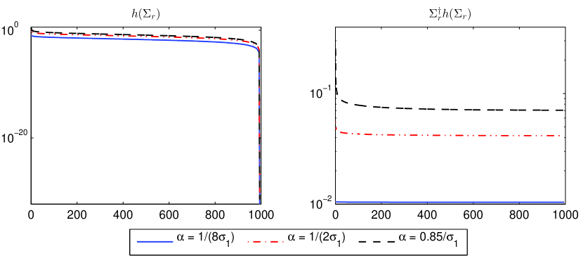
Fig. 1: Network: Roget. Diagonal entries of $h(\Sigma_{r})$ and $\Sigma_{r}^{\dagger}h(\Sigma_{r})$ for $h(t)=\frac{\alpha t}{1-(\alpha t)^{2}}$, when $\alpha=\frac{1}{8\sigma_{1}},\frac{1}{2\sigma_{1}},0.85\ \sigma_{1}^{-1}$

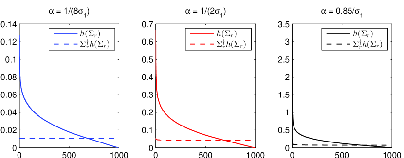
Fig. 2: Network: Roget. Diagonal entries of $h(\Sigma_{r})$ and $\Sigma_{r}^{\dagger}h(\Sigma_{r})$ for $h(t)=\frac{\alpha t}{1-(\alpha t)^{2}}$, when $\alpha=\frac{1}{8\sigma_{1}},\frac{1}{2\sigma_{1}},0.85\ \sigma_{1}^{-1}$

Table 4: Network: Roget, $h(t)=\frac{\alpha t}{1-(\alpha t)^{2}}$, $\alpha=\frac{1}{8\sigma_{1}}$ (${\rm tol}=10^{-4}$).

	First approach		Second approach		Third approach
	ITER	${\pcal E}_{\ell}$	ITER	${\pcal E}_{\ell}$	ITER	${\pcal E}_{\ell}$
1	75	2.14e+03	75	2.14e+03	5	6.61e-08
2	106	1.60e-02	106	1.60e-02	4	3.75e-08
3	906	2.99e-01	906	2.99e-01	5	1.65e-08
4	992	2.17e-08	992	7.82e-06	5	1.33e-07
5	166	7.16e+02	166	7.16e+02	5	7.52e-08
6	257	1.03e-01	257	1.03e-01	4	4.46e-08
7	874	5.41e-01	874	5.41e-01	5	2.46e-08
8	274	1.06e+00	274	1.06e+00	5	9.46e-08
9	259	8.37e-04	259	8.37e-04	5	7.31e-11
10	733	2.48e+01	733	2.48e+01	5	3.37e-07

Table 5: Network: Roget, $h(t)=\frac{\alpha t}{1-(\alpha t)^{2}}$, $\alpha=\frac{1}{2\sigma_{1}}$ (${\rm tol}=10^{-4}$).

	First approach		Second approach		Third approach
	ITER	${\pcal E}_{\ell}$	ITER	${\pcal E}_{\ell}$	ITER	${\pcal E}_{\ell}$
1	75	6.32e+00	75	6.32e+00	7	1.90e-06
2	87	8.90e-03	87	8.90e-03	6	6.02e-07
3	308	1.10e-02	308	1.10e-02	6	7.96e-06
4	106	5.71e-01	106	5.72e-01	7	7.77e-08
5	495	1.72e-01	495	1.72e-01	7	4.43e-06
6	79	4.51e-02	79	4.51e-02	6	2.12e-06
7	118	8.64e-02	118	8.64e-02	7	4.24e-07
8	121	1.00e-01	121	1.01e-01	7	5.84e-07
9	59	1.91e-02	59	1.91e-02	6	6.99e-07
10	574	1.87e-01	574	1.87e-01	7	1.49e-06

Table 6: Network: Roget, $h(t)=\frac{\alpha t}{1-(\alpha t)^{2}}$, $\alpha=0.85\ \sigma_{1}^{-1}$ (${\rm tol}=10^{-4}$).

	First approach		Second approach		Third approach
	ITER	${\pcal E}_{\ell}$	ITER	${\pcal E}_{\ell}$	ITER	${\pcal E}_{\ell}$
1	74	2.72e-01	74	2.72e-01	10	4.88e-06
2	66	3.45e-03	66	3.45e-03	8	5.22e-06
3	97	6.96e-02	97	6.96e-02	8	4.79e-06
4	58	3.72e-02	58	3.72e-02	8	8.04e-05
5	147	6.23e-02	147	6.23e-02	9	1.23e-05
6	53	8.48e-03	53	8.48e-03	9	3.34e-06
7	74	1.58e-02	74	1.58e-02	7	3.20e-04
8	117	6.49e-03	117	6.49e-03	10	4.52e-06
9	23	6.02e-03	23	6.02e-03	9	4.34e-07
10	152	1.70e-01	152	1.70e-01	9	3.90e-05

Comparison with standard Lanczos-based approach

In the case of generalized matrix functions like $\sinh^{\diamond}(A)$, which occur as submatrices of “standard” matrix functions applied to the symmetric matrix $\mathscr{A}$, it is natural to compare the previously proposed approaches with the use of Gauss quadrature-based bounds and estimates based on the Lanczos process. This was the approach used, for example, in [4]. Henceforth, we refer to this approach as “the mmq approach,” since it is implemented on the basis of the ${\tt mmq}$ toolkit [22] originally developed by Gérard Meurant; see also [12].

Numerical experiments, not shown here, indicate that on average, the mmq approach requires a slightly higher number of iterations than our third approach to deliver comparable accuracy in computing the communicability between pairs of nodes. Note that the cost per step is comparable for the two methods. An advantage of the mmq approach is that it can provide lower and upper bounds on the quantities being computed, but only if bounds on the singular values of $A$ are available. A disadvantage is that it requires working with vectors of length $2n$ instead of $n$.

Of course, the Lanczos-based approach is not applicable to generalized matrix functions that do not arise as submatrices of standard matrix functions.

Block approaches

In the following, we test the performance of the two block approaches described in section 6 when trying to approximate the communicabilities among $k$ nodes of the Twitter network, which has $3656$ nodes and $188712$ edges [25]. All the computations were carried out with MATLAB Version 7.10.0.499 (R2010a) 64-bit for Linux, in double precision arithmetic, on an Intel Core i5 computer with 4 GB RAM.

In order to compute approximations to the communicabilities, we set

$$Z=W=[\mathbf{e}_{i_{1}},{\bf e}_{i_{2}},\dots,\mathbf{e}_{i_{k}}],$$

where $i_{1},i_{2},\dots,i_{k}$ are chosen uniformly at random among the $n$ nodes of the network. To better analyze the behavior of the methods, we run both algorithms ten times and report in each table the averaged values obtained by changing the set of $k$ nodes after each run. As in the previous subsection, we test the performance of the two generalized matrix functions induced by $h(t)=\sinh(t)$ and $h(t)=\alpha t(1-(\alpha t)^{2})^{-1}$, respectively.

The first approach is based on the computation of block Gauss and anti-Gauss quadrature rules. Since $\widetilde{Z}\neq W$, we need to use the nonsymmetric Lanczos algorithm and, in order to avoid breakdown during the computation, it is convenient to add a dense vector to each initial block (see [2] for more details). Each table reports the relative error and the relative distance between the two quadrature rules computed as:

$${\pcal E}_{\ell}=\frac{\|F_{\ell}-Z^{T}h^{\diamond}(A)W\|_{2}}{\|Z^{T}h^{\diamond}(A)W\|_{2}}\qquad\text{and}\qquad{\pcal R}_{\ell}=\frac{\|{\pcal G}_{\ell}-{\pcal H}_{\ell+1}\|_{\max}}{\|{\pcal G}_{\ell}+{\pcal H}_{\ell+1}\|_{\max}}\,,$$

respectively, where

$$\|M\|_{\max}=\smash{\displaystyle\max_{\begin{subarray}{c}1\leq i\leq m\\ 1\leq j\leq n\end{subarray}}}\{M_{ij}\}\text{, with }M\in{{\mathbb{C}}^{m\times n}},$$

and $F_{\ell}$ is given by (13).

In order to obtain good entrywise approximations of $Z^{T}h^{\diamond}(A)W$, the domain $D$ of analyticity of $g(t)=(\sqrt{t})^{-1}h(\sqrt{t})$ has to enclose the smallest interval containing the spectrum of $A^{T}A$, and the boundary $\partial D$ has to be well separated from the extremes of the interval. However, when $h(t)=\sinh(t)$, the function $g(t)$ applied to our test problems does not exhibit this nice property; indeed, in all three cases $A$ is (numerically) singular and therefore the singularity $t=0$ belongs to the smallest interval containing the spectrum $A^{T}A$. As pointed out in section 6, we cannot therefore expect $F_{\ell}=\left({\pcal G}_{\ell}+{\pcal H}_{\ell+1}\right)/2$ to provide a good approximation for $Z^{T}h^{\diamond}(A)W$, since the condition $\left({\pcal I}-{\pcal H}_{\ell+1}\right)g\approx-\left({\pcal I}-{\pcal G}_{\ell}\right)g$ is not guaranteed.

The results in Table 7 confirm this observation, since they clearly show that the relative error ${\pcal E}_{\ell}$ is not comparable with the relative distance ${\pcal R}_{\ell}$. As expected, a small value of ${\pcal R}_{\ell}$ does not ensure a satisfactory value of ${\pcal E}_{\ell}$. Therefore, the relative distance between the approximations provided by the Gauss and anti-Gauss rules cannot be used as a stopping criterion. Moreover, the results in Table 7 also show that performing more iterations does not improve the results; indeed, for all the values of the block size $k$ it holds ${\pcal E}_{5}\approx{\pcal E}_{10}$. It is also worth noting that the relative distance does not decrease as $\ell$ increases, but stabilizes far from the desired value and in one case it even increases. In view of this, the behavior of the algorithm is not satisfactory regardless of the nodes taken into account or the block size $k$.

Table 7: Execution time (in seconds), relative error and relative distance for the computation of the total communicabilities between $k$ nodes of the Twitter network with $\ell=5$ and $\ell=10$ steps.

$k$	$\ell=5$			$\ell=10$
	Time	${\pcal E}_{5}$	${\pcal R}_{5}$	Time	${\pcal E}_{10}$	${\pcal R}_{10}$
5	2.14e-01	4.62e-04	5.07e-09	3.50e-01	4.62e-04	9.74e-10
10	2.70e-01	1.04e-02	2.21e-09	5.62e-01	1.04e-02	9.96e-10
20	4.21e-01	3.78e-02	5.39e-10	1.10e+00	3.78e-02	8.12e-09
30	6.63e-01	2.24e-02	1.78e-11	2.12e+00	2.24e-02	3.14e-10
50	1.24e+00	4.59e-02	6.83e-12	5.57e+00	4.59e-02	1.63e-11
100	3.86e+00	5.65e-02	3.43e-11	2.72e+01	5.65e-02	1.60e-11

Tables 8–10 report the performance of the method when trying to approximate the communicabilities with respect to the function $h(t)=\alpha t(1-(\alpha t)^{2})^{-1}$, using different values of $\alpha\in(0,\sigma_{1}^{-1})$. In this case, the function $g(t)=\alpha(1-\alpha^{2}t)^{-1}$ is analytic, provided that $\alpha<\sigma_{1}^{-1}$, as in our case.

Note that as $\alpha$ approaches $\sigma_{1}^{-1}$, the relative error ${\pcal E}_{\ell}$ increases (cf. Tables 8–10). This happens because the distance between the boundary $\partial D$ of the domain $D$ of analyticity of $g(t)$ and the smallest interval containing the spectrum of $A^{T}A$ is decreasing (see section 6.1). In the first table, the values of ${\pcal E}_{2}$ and ${\pcal R}_{2}$ are comparable and we reach the desired accuracy with only two iterations. We remark that some other experiments, not shown here, pointed out that increasing the number of steps of the algorithm does not improve the relative error.

Table 8: Number of block Lanczos steps, execution time (in seconds), relative error and relative distance for the computation of the Katz communicabilities between $k$ nodes of the Twitter network. Here, $\alpha=1/(8\sigma_{1})$.

$k$	Time	${\pcal E}_{2}$	${\pcal R}_{2}$
5	5.20e-02	4.77e-04	1.99e-04
10	8.89e-02	7.90e-05	2.85e-04
20	1.69e-01	4.06e-04	2.59e-04
30	2.71e-01	5.85e-04	1.50e-04
50	1.31e+00	2.60e-04	1.53e-04
100	6.75e-01	5.40e-04	1.83e-04

Table 9: Number of block Lanczos steps, execution time (in seconds), relative error and relative distance for the computation of the Katz communicabilities between $k$ nodes of the Twitter network. Here, $\alpha=1/(2\sigma_{1})$.

$k$	Time	${\pcal E}_{3}$	${\pcal R}_{3}$
5	5.63e-02	6.20e-04	7.54e-05
10	9.47e-02	4.50e-04	2.66e-05
20	1.79e-01	3.36e-03	1.15e-05
30	2.61e-01	2.41e-03	6.56e-07
50	4.66e-01	8.36e-03	1.14e-06
100	1.35e+00	9.21e-03	1.04e-07

Table 10: Number of block Lanczos steps, execution time (in seconds), relative error and relative distance for the computation of the communicabilities between $k$ nodes of the Twitter network. Here, $\alpha=0.85/\sigma_{1}$.

$k$	Time	${\pcal E}_{3}$	${\pcal R}_{3}$
5	8.07e-02	1.89e-03	5.04e-05
10	9.74e-02	4.26e-03	2.76e-04
20	1.83e-01	2.19e-02	3.25e-04
30	2.95e-01	1.45e-02	6.48e-05
50	5.27e-01	3.46e-02	7.41e-05
100	1.33e+00	1.90e-02	7.27e-06

Table 9 shows that we obtain good approximations setting $\alpha=0.5\sigma_{1}^{-1}$, but the relative distance between the two quadrature rules decreases faster than the relative error. A similar behavior is shown in Table 10, where $\alpha=0.85\sigma_{1}^{-1}$. The relative error increases as $\alpha$ gets closer to $\sigma_{1}^{-1}$ and does not improve performing more steps.

Table 11: Execution time (in seconds), relative error, number of block GK steps and stopping criterion for the computation of the communicabilities between $k$ nodes of the Twitter network.

$k$	ITER	Time	${\pcal E}_{\ell}$	${\pcal R}_{\ell}$
5	6	2.51e+00	1.14e-08	1.98e-06
10	6	1.65e+00	5.79e-09	1.58e-06
20	5	1.77e+00	5.21e-09	1.20e-06
30	5	2.19e+00	5.05e-09	1.25e-06
50	5	3.34e+00	1.84e-09	7.04e-07
100	4	5.05e+00	6.65e-09	4.38e-06

We turn now to the approximation of the quantity (6) using the second block approach, namely the block Golub–Kahan decomposition algorithm. When using this approach, we perform as many steps as necessary to obtain

$${\pcal R}_{\ell}=\frac{\|F_{\ell}-F_{\ell-1}\|_{2}}{\|F_{\ell-1}\|_{2}}<{\rm tol},$$

with ${\rm tol}=10^{-5}$. Table 11 displays the results obtained when we approximate the communicabilities among $k$ nodes with respect to the generalized matrix function induced by $h(t)=\sinh(t)$. Clearly, this approach requires a small number of steps to reach a high level of accuracy.

Table 12: Execution time (in seconds), relative error, number of block Golub–Kahan steps and stopping criterion for the computation of the communicabilities among $k$ nodes of the Twitter network. In this case, $\alpha=1/(8\sigma_{1})$.

$k$	ITER	Time	${\pcal E}_{\ell}$	${\pcal R}_{\ell}$
5	3	7.62e-01	3.22e-10	2.14e-06
10	3	8.01e-01	3.93e-10	2.16e-06
20	3	9.27e-01	1.77e-10	2.24e-06
30	3	1.09e+00	9.64e-11	1.74e-06
50	3	1.49e+00	4.40e-11	6.70e-07
100	3	2.86e+00	1.16e-11	4.21e-07

Table 13: Execution time (in seconds), relative error, number of block GK steps and stopping criterion for the computation of the communicabilities between $k$ nodes of the Twitter network. In this case, $\alpha=1/(2\sigma_{1})$.

$k$	ITER	Time	${\pcal E}_{\ell}$	${\pcal R}_{\ell}$
5	4	9.35e-01	3.47e-08	2.05e-06
10	4	1.08e+00	8.85e-09	1.90e-06
20	4	1.38e+00	1.56e-09	1.20e-06
30	4	1.65e+00	3.70e-10	3.59e-07
50	4	2.32e+00	1.49e-10	2.56e-07
100	4	4.91e+00	2.20e-11	6.21e-08

Table 14: Execution time (in seconds), relative error, number of block GK steps and stopping criterion for the computation of the communicabilities between $k$ nodes of the Twitter network. In this case, $\alpha=0.85/\sigma_{1}$.

$k$	ITER	Time	${\pcal E}_{\ell}$	${\pcal R}_{\ell}$
5	5	1.29e+00	3.02e-08	2.08e-06
10	5	1.36e+00	1.01e-08	6.86e-07
20	5	1.66e+00	1.42e-08	2.38e-06
30	5	2.16e+00	3.49e-09	1.33e-06
50	4	2.58e+00	7.81e-09	4.33e-06
100	4	4.84e+00	1.73e-09	1.62e-06

Tables 12-14 show the results concerning the approximation of the communicabilities among $k$ nodes using the generalized matrix function induced by $h(t)=\alpha t(1-(\alpha t)^{2})^{-1}$. As above, we consider three different values for the parameter $\alpha$. As in the scalar case, the method requires fewer iterations to reach a higher accuracy as the value of $\alpha$ moves away from $\sigma_{1}^{-1}$.

The two approaches behave again very differently. As before, the results obtained with the second approach are very promising also in view of the fact that we did not make any assumptions on the regularity of the function.

8 Conclusions

In this paper we have proposed several algorithms for the computation of certain quantities associated with generalized matrix functions. These techniques are based on Gaussian quadrature rules and different variants of the Lanczos and Golub–Kahan algorithms. In particular, we have investigated three distinct approaches for estimating scalar quantities like ${\bf z^{T}}f^{\diamond}(A){\bf w}$, and two block methods for computing matrix-valued expressions like $Z^{T}f^{\diamond}(A)W$. The performance of the various approaches has been tested in the context of computations arising in network theory. While not all methods can be expected to always perform well in practice, we have identified two approaches (one scalar-based, the other block-based) that produce fast and accurate approximations for the type of problems considered in this paper.

References

- [1] F. Arrigo and M. Benzi, Edge modification criteria for enhancing the communicability of digraphs, arXiv:1508.01056v2, November 2015.
- [2] Z. Bai, D. Day, and Q. Ye, ABLE: An adaptive block Lanczos method for non-Hermitian eigenvalue problems, SIAM J. Matrix Anal. Appl., 20 (1999), pp. 1060–1082.
- [3] V. Batagelj and A. Mrvar, Pajek datasets, http://vlado.fmf.uni-lj.si/pub/networks/data/.
- [4] M. Benzi, E. Estrada, and C. Klymko, Ranking hubs and authorities using matrix functions, Linear Algebra Appl., 438 (2013), pp. 2447–2474.
- [5] D. Calvetti, L. Reichel, and F. Sgallari, Application of anti-Gauss quadrature rules in linear algebra, Applications and Computation of Orthogonal Polynomials, W. Gautschi, G. H. Golub, and G. Opfer, eds., Birkhäuser, Basel, 1999, pp. 41–56.
- [6] J. J. Crofts, E. Estrada, D. J. Higham, and A. Taylor, Mapping directed networks, Electron. Trans. Numer. Anal., 37 (2010), pp. 337–350.
- [7] T. Davis and Y. Hu, The University of Florida Sparse Matrix Collection, \urlhttp://www.cise.ufl.edu/research/sparse/matrices/.
- [8] N. Del Buono, L. Lopez, and R. Peluso, Computation of the exponential of large sparse skew-symmetric matrices, SIAM J. Sci. Comput., 27 (2005), pp. 278–293.
- [9] N. Del Buono, L. Lopez and T. Politi, Computation of functions of Hamiltonian and skew-symmetric matrices, Math. Comp. Simul., 79 (2008), pp. 1284–1297.
- [10] C. Fenu, D. Martin, L. Reichel, and G. Rodriguez, Block Gauss and anti-Gauss quadrature with application to networks, SIAM J. Matrix Anal. Appl., 34 (2013), pp. 1655-1684.
- [11] G. H. Golub and W. Kahan, Calculating the singular values and pseudo-inverse of a matrix, SIAM J. Numer. Anal., 2 (1965), pp. 205–224.
- [12] G. H. Golub and G. Meurant, Matrices, Moments and Quadrature with Applications, Princeton University Press, Princeton, NJ, 2010.
- [13] G. H. Golub and C. F. Van Loan, Matrix Computations. Fourth Edition, Johns Hopkins University Press, Baltimore and London, 2013.
- [14] M. Hanke, J. Nagy, and R. Plemmons, Preconditioned iterative regularization for ill-posed problems, in L. Reichel, A. Ruttan, and R. S. Varga, Eds., Numerical Linear Algebra. Proceedings of the Conference in Numerical Linear Algebra and Scientific Computation, Kent, Ohio, USA, March 13–14, 1992, de Gruyter, Berlin and New York, 1993, pp. 141–163.
- [15] J. B. Hawkins and A. Ben–Israel, On generalized matrix functions, Linear and Multilinear Algebra, 1 (1973), pp. 163–171.
- [16] N. J. Higham, Functions of Matrices. Theory and Computation, Society for Industrial and Applied Mathematics, Philadelphia, PA, 2008.
- [17] R. A. Horn and C. R. Johnson, Matrix Analysis. Second Edition, Cambridge University Press, 2013.
- [18] L. Katz, A new status index derived from sociometric data analysis, Psychometrika, 18 (1953), pp. 39–43.
- [19] D. P. Laurie, Anti-Gaussian quadrature formulas, Math. Comp., 65 (1996), pp. 739–747.
- [20] L. Lopez and A. Pugliese, Decay behaviour of functions of skew-symmetric matrices, in Proceedings of HERCMA 2005, 7th Hellenic-European Conference on Computer Mathematics and Applications, September, 22-24, 2005, Athens, E. A. Lipitakis, ed., Electronic Editions LEA, Athens.
- [21] J. R. Magnus and H. Neudecker, Matrix Differential Calculus with Applications in Statistics and Econometrics, Wiley, NY, 1988.
- [22] G. Meurant, MMQ toolbox for MATLAB, http://pagesperso-orange.fr/gerard.meurant/.
- [23] K. S. Miller and G. Samko, Completely monotonic functions, Integr. Transf. and Spec. Funct., 4 (2001), pp. 389–402.
- [24] L. Muchnik, Lev Muchnik’s data sets web page, \urlhttp://www.levmuchnik.net/Content/Networks/NetworkData.html.
- [25] SNAP Network Data Sets, \urlhttp://snap.stanford.edu/data/index.html.
- [26] D. V. Widder, The Laplace Transform, Princeton University Press, Princeton, NJ, 1946.