Impulse-Induced Optimum Signal Amplification in Scale-Free Networks

Abstract

Optimizing information transmission across a network is an essential task for controlling and manipulating generic information-processing systems. Here, we show how topological amplification effects in scale-free networks of signaling devices are optimally enhanced when the impulse transmitted by periodic external signals (time integral over two consecutive zeros) is maximum. This is demonstrated theoretically by means of a star-like network of overdamped bistable systems subjected to generic zero-mean periodic signals, and confirmed numerically by simulations of scale-free networks of such systems. Our results show that the enhancer effect of increasing values of the signal’s impulse is due to a correlative increase of the energy transmitted by the periodic signals, while it is found to be resonant-like with respect to the topology-induced amplification mechanism.

Introduction.$-$Today, there is an emerging ”network perspective” approach to studying complex systems reflecting the ubiquitous presence of networks in nature and in human societies. In particular, there has been considerable interest in a class of networks known as scale-free networks due to their lack of a characteristic size [1-4]. They have the property that the degrees, $\kappa$, of the node follow a scale-free power-law distribution $\left(P\left(\kappa\right)\sim\kappa^{-\gamma},\gamma\in[2,3]\right)$. Examples are diverse metabolic and cellular networks, computer networks such as the World Wide Web, and some social examples such as collaboration networks. Besides topological investigations [5,6], current interest in these (and other) networks has extended to their controllability [7,8], i.e., to the characterization and control of the dynamical properties of processes occurring in them, such as transport [9], synchronization of individual dynamical behaviour occurring at a network’s vertices [10,11], role of quenched spatial disorder in the optimal path problem in weighted networks [12], and dynamic pattern evolution [13]. One particular issue that has attracted much interest because of its importance in both biological and man-made information-processing systems is the propagation and enhancement of resonant collective behaviour across a network due to the application of weak external signals. In this regard, there has been recently studied the amplification of the response to weak harmonic signals in networks of bistable signaling devices [14-17]. In these works, however, the robustness of the signal amplification against diversity in the uniform distributions of periodic external signals was not studied. Clearly, the assumption of harmonic external signals means that all driving systems$-$whatever they might be$-$are effectively taken as linear. This mathematically convenient choice is untenable for most natural and artificial information-processing systems due to their irreducible nonlinear nature. Thus, to approach signal amplification phenomena in real-world networks, it seems appropriate to consider distributions of periodic external signals which are the output of nonlinear systems, therefore being appropriately represented by generic Fourier series.

In this Letter, we study the interplay between heterogeneous connectivity, quenched spatial disorder, and generic zero-mean periodic signals in random scale-free networks of signaling devices through the instance of a simple deterministic overdamped bistable system. The system is given by

$$\overset{.}{x}_{i} =x_{i}-x_{i}^{3}+\tau f(t)-\lambda L_{ij}x_{j,}\;i=1,...,N,$$

$$f(t) \equiv\sum_{n=1}^{\infty}a_{n}\sin\left(2n\pi t/T+\varphi_{n}\right),$$ (1)

where $f(t)$ is a unit-amplitude, zero-mean, $T$-periodic signal, $\tau$ is the signal amplitude, $\lambda$ is the coupling, $L_{ij}=\kappa_{i}\delta_{ij}-A_{ij}$ is the Laplacian matrix of the network, $\kappa_{i}=\sum_{j}A_{ij}$ is the degree of node $i$, and $A_{ij}$ is the adjacency matrix with entries 1 if $i$ is connected to $j$, and 0 otherwise. Since there are infinitely many a priori independent parameters, $a_{n}$, $\varphi_{n}$, and hence infinitely many different waveforms of $f(t)$, the relevant problem is how to characterize quantitatively the effect of the signal’s waveform on the topology-induced amplification scenario [14]. Here, we shall show that a relevant quantity properly characterizing the effectiveness of generic periodic signals (1) in the amplification scenario is the impulse transmitted by the signal over a half-period (hereafter referred to simply as the impulse, $I\equiv\tau\int_{0}^{T/2}f(t)dt$) $-$ a quantity integrating the conjoint effects of the signal’s amplitude, period, and waveform (see Fig. 1 for an example). Remarkably, we found that the enhancer effect of increasing values of the impulse is due to a correlative increase of the energy transmitted by the periodic signals. Extensive numerical simulations of the system (1) were conducted for different network topologies to characterize the effect of the impulse on the amplification-synchronization scenario as the coupling strength is increased.

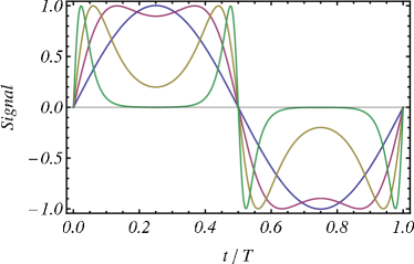
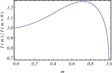
Figure 1: (Color online) Top: Signal $f\left(t;T,m\right)$ [Eq. (12)] vs $t/T$ where $T$ is the period and $N(m)\equiv 1/\left\{a+b/[1+\exp(\left\{m-c\right\}/d)]\right\}$ with $a\equiv 0.43932$, $b\equiv 0.69796$, $c\equiv 0.3727$, $d\equiv 0.26883$ for four values of the shape parameter: $m=0$ (sinusoidal pulse), $m=0.72\simeq m_{\max}$ (nearly square-wave pulse), $m=0.99$ (double-humped pulse), and $m=1-10^{-6}$ (sharp double-humped pulse). Bottom: The normalized impulse $I(m,T)/I(0,T)$ [Eq. (13)] vs $m$.

To quantitatively describe this scenario, we used the average amplification $\left\langle G\right\rangle\equiv\max_{i}x_{i}/\tau$ over distinct initial conditions on the one hand, and the synchronization coefficient [18]

$$\rho=\frac{\left\langle\overline{x_{i}}^{2}\right\rangle-\left\langle\overline{x_{i}}\right\rangle^{2}}{\overline{\left\langle x_{i}^{2}\right\rangle-\left\langle x_{i}\right\rangle^{2}}},$$ (2)

on the other, where the overlines indicate an average over nodes, while the angle brackets indicate a temporal average over a period $T$.

Energy variation versus impulse.$-$We start with a general argument showing the relationship between energy increases and impulse increases in isolated overdamped systems. Let us consider the family of dissipative nonlinear oscillators $m\overset{..}{x}=-dU/dx-\delta\overset{.}{x}+\tau f(t)$, with associated energy equation $\overset{.}{E}=\overset{.}{x}\left(m\overset{..}{x}+dU/dx\right)$, where $f(t)$ is a unit-amplitude, zero-mean, $T$-periodic signal, $E(t)\equiv\left(m/2\right)\overset{.}{x}^{2}+U\left[x\left(t\right)\right]$ is the energy function with $U$ being a generic potential. The energy equation can be recast into the form

$$\overset{.}{E}=-\delta\overset{.}{x}^{2}+\tau\overset{.}{x}f\left(t\right).$$ (3)

Integration of Eq. (3) over any interval $\left[nT,nT+T/2\right]$, $n=0,1,2,...$, yields

$$E\left(nT+T/2\right) =E\left(nT\right)-\delta\int_{nT}^{nT+T/2}\overset{.}{x}^{2}\left(t\right)dt$$

$$+\tau\int_{nT}^{nT+T/2}\overset{.}{x}\left(t\right)f(t)dt.$$ (4)

Now, after applying the first mean value theorem for integration [19] to the last integral on the right-hand side of Eq. (4), one straightforwardly obtains

$$E\left(nT+T/2\right)=E\left(nT\right)-\delta\int_{nT}^{nT+T/2}\overset{.}{x}^{2}\left(t\right)dt+\overset{.}{x}\left(t^{\ast}\right)I,$$ (5)

where $t^{\ast}\in\left[nT,nT+T/2\right]$ and $I$ is the impulse. Let us consider an initial steady ($n$ large) situation fixing the parameters $\left(\delta,\tau,T\right)$ and choosing a waveform such that the impulse is relatively small. Next, we only change the waveform. For sufficiently small values of $T$ and $\tau$, one expects that both the dissipation work (integral in Eq. (5)) and $\overset{.}{x}\left(t^{\ast}\right)$ will approximately maintain their initial values, while $I$ may increase from its initial value with the choice of a more convenient waveform, so that, in some cases depending upon the remaining parameters, the energy difference $E\left(nT+T/2\right)-E\left(nT\right)$ will increase with respect to the initial situation. Thus, the maximum probability of a maximal increase of the energy difference occurs when $I$ is also maximum, which establishes a clear correlation between impulse and energy transmitted over wide regions in parameter space. Specifically, one expects this impulse principle to be accurate when the signal period is the shortest significant timescale. Numerical simulations confirmed the accuracy and scope of this prediction. Figure 2 shows an illustrative example for an isolated overdamped bistable system (cf. Eq. (1)).

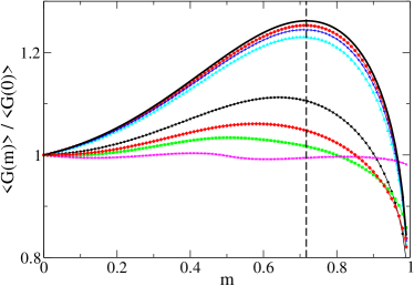
Figure 2: (Color online) Normalized average amplification $\left\langle G(m)\right\rangle/\left\langle G(m=0)\right\rangle$ versus shape parameter $m$ for an isolated overdamped bistable system [Eq. (1) with $\lambda=0$] subjected to a signal given by Eq. (12) and seven values of the signal period: $T=1/\sqrt{2}$ (circles), $T=1\left(+\right)$, $T=\sqrt{2}$ (triangles), $T=2\pi/\sqrt{2}\left(\ast\right)$, $T=7$ (diamonds), $T=10$ (squares), and $T=50\left(\times\right)$. The solid line shows the normalized impulse $I(m,T)/I(0,T)$ [Eq. (13)] versus shape parameter $m$ while the dashed vertical line indicates the value $m=m_{\max}\simeq 0.717$ for which $I(m,T)/I(0,T)$ presents its single maximum as a function of $m$. Notice that the period of the linearized motion around any of the potential minima, $T=2\pi/\sqrt{2}$, corresponds to the shortest significant timescale.

Star-like network.$-$Next, we consider a star-like network of overdamped bistable systems:

$$\overset{.}{x}_{H} =\left[1-\lambda\left(N-1\right)\right]x_{H}-x_{H}^{3}+\tau f(t)+\lambda\sum_{i=1}^{N-1}y_{i},$$

$$\overset{.}{y}_{i} =\left(1-\lambda\right)y_{i}-y_{i}^{3}+\tau f(t)+\lambda x_{H},$$ (6)

which describes the dynamics of a highly connected node (or hub), $x_{H}$, and $N-1$ linked systems (or leaves), $y_{i}$. We study the case of sufficiently small coupling, $\lambda$, and external signal amplitude, $\tau$, such that the dynamics of the leaves may both be decoupled from that of the hub and be suitably described by linearizing their equations around one of the potential minima. Thus, one straightforwardly obtains

$$y_{i}\left(t\rightarrow\infty\right) \sim\xi_{i}-\tau\sum_{n=1}^{\infty}\left[C_{n}\cos\left(\omega_{n}t\right)+S_{n}\sin\left(\omega_{n}t\right)\right],$$

$$C_{n} \equiv\frac{a_{n}\left(\omega_{n}\cos\varphi_{n}-2\sin\varphi_{n}\right)}{\omega_{n}^{2}+4},$$

$$S_{n} \equiv-\frac{a_{n}\left(\omega_{n}\sin\varphi_{n}+2\cos\varphi_{n}\right)}{\omega_{n}^{2}+4},$$ (7)

where $\omega_{n}\equiv 2n\pi/T$ while $\xi_{i}=\pm 1$ depending on the initial conditions. Since the initial conditions are randomly chosen, this means that the quantities $\xi_{i}$ behave as discrete random variables governed by Rademacher distributions. After inserting Eq. (7) into Eq. (6) and solving the resulting equation for the hub,

$$\overset{.}{x}_{H}= \left[1-\lambda\left(N-1\right)\right]x_{H}-x_{H}^{3}+\sum_{n=1}^{\infty}\left[C_{n}^{\prime}\cos\left(\omega_{n}t\right)\right.$$

$$\left.+S_{n}^{\prime}\sin\left(\omega_{n}t\right)\right]+\lambda\eta,$$ (8)

where

$$\eta \equiv\sum_{i=1}^{N-1}\xi_{i},$$

$$\frac{C_{n}^{\prime}}{\tau} \equiv a_{n}\left(1+\frac{2\lambda\left(N-1\right)}{\omega_{n}^{2}+4}\right)\sin\varphi_{n}-\frac{\lambda\left(N-1\right)a_{n}\omega_{n}}{\omega_{n}^{2}+4}\cos\varphi_{n},$$

$$\frac{S_{n}^{\prime}}{\tau} \equiv\frac{\lambda\left(N-1\right)a_{n}\omega_{n}}{\omega_{n}^{2}+4}\sin\varphi_{n}+a_{n}\left(1+\frac{2\lambda\left(N-1\right)}{\omega_{n}^{2}+4}\right)\cos\varphi_{n},$$

one straightforwardly obtains

$$x_{H}\left(t\rightarrow\infty\right) \sim x_{H}^{(0)}+\sum_{n=1}^{\infty}\left[\frac{\left(C_{n}^{\prime}\omega_{n}+S_{n}^{\prime}a_{H}\right)\sin\left(\omega_{n}t\right)}{\omega_{n}^{2}+a_{H}^{2}}\right.$$

$$\left.+\frac{\left(C_{n}^{\prime}a_{H}-S_{n}^{\prime}\omega_{n}\right)\cos\left(\omega_{n}t\right)}{\omega_{n}^{2}+a_{H}^{2}}\right],$$ (9)

where $a_{H}\equiv V_{H}^{\prime\prime}\left(x_{H}^{(0)}\right)=-\left\{\frac{3\lambda\eta}{x_{H}^{(0)}}+2\left[1-\lambda\left(N-1\right)\right]\right\}$ with $x_{H}^{(0)}$ being the equilibrium in the absence of any external signal, while $V_{H}(x_{H})\equiv-\sqrt{h}x_{H}^{2}+x_{H}^{4}/4$ is the hub potential with $h=\left[1-\left(N-1\right)\lambda\right]^{2}/4$ being the height of the potential barrier. For finite $N$, the quantity $\eta$ behaves as a discrete random variable governed by a binomial distribution with zero mean and variance $N-1$. One sees that the hub’s dynamics is affected by spatial quenched disorder through the term $\lambda\eta$, while an estimate of its amplification [20] is given by

$$G\left[f(t)\right]=\frac{1}{\tau}\left(\sum_{n=1}^{\infty}\frac{C_{n}^{\prime 2}+S_{n}^{\prime 2}}{\omega_{n}^{2}+a_{H}^{2}}\right)^{1/2}.$$ (10)

For sufficiently large $N$, we may assume that the quantity $\eta$ behaves as a continuous random variable governed by a standard normal distribution, and hence

$$\left\langle G\right\rangle=\frac{1}{\sqrt{2\pi\left(N-1\right)}}\int_{-\infty}^{\infty}G\left[f(t)\right]\exp\left[\frac{-\eta^{2}}{2\left(N-1\right)}\right]d\eta$$ (11)

provides the final average amplification. Next, we demonstrate that the impulse is the relevant quantity controlling the effect of the external signal on the amplification by considering the illustrative example

$$f\left(t;T,m\right)\equiv N(m)\operatorname{sn}\left(4Kt/T\right)\operatorname*{dn}\left(4Kt/T\right),$$ (12)

in which $\operatorname{sn}\left(\cdot\right)\equiv\operatorname{sn}\left(\cdot;m\right)$ and $\operatorname*{dn}\left(\cdot\right)\equiv\operatorname*{dn}\left(\cdot;m\right)$ are Jacobian elliptic functions of parameter $m$ [$K\equiv K(m)$ is the complete elliptic integral of the first kind] [21] and $N(m)$ is a normalization function (see Fig. 1, top) which is introduced for the elliptic signal to have the same amplitude 1 and period $T$ for any wave form (i.e., $\forall m\in\left[0,1\right]$). When $m=0$, then $f\left(t;T,m=0\right)=\sin\left(2\pi t/T\right)$, i.e., one recovers the previously studied case of a harmonic signal [14], whereas, for the limiting value $m=1$, the signal vanishes. Note that, as a function of $m$, the impulse per unit of amplitude,

$$I\mid_{\tau=1}=I(m,T)\equiv\frac{TN(m)}{2K(m)}$$ (13)

presents a single maximum at $m=m_{\max}\simeq 0.717$ (see Fig. 1, bottom). In this case, Eq. (11) predicts that $\left\langle G\right\rangle\left(\lambda,N,T,m=m_{\max}\right)>\left\langle G\right\rangle\left(\lambda,N,T,m\neq m_{\max}\right)$ and that the signal amplification increases on average as the impulse is increased, i.e., as the shape parameter $m\rightarrow m_{\max}$ (see Fig. 3, left), which is accurately confirmed by numerical simulations (see Fig. 3, right). One also has from Eqs. (11) and (12) that $\left\langle G\right\rangle\left(\lambda,N,T,m\right)$, as a function of only $\lambda$, presents a sharp single maximum at $\lambda=\lambda_{\max}\simeq\left(N-1\right)^{-1}$for all $m$, which indicates that the topology-induced amplification mechanism is robust against diversity in the uniform distributions of periodic signals in star-like networks.

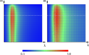
Figure 3: (Color online) Theoretical average amplification $\left\langle G\right\rangle$ in the $\left(\lambda-m\right)$ parameter plane (left panel, Eqs. (11) and (12)) and corresponding numerical results $\left\langle G\right\rangle$ (right panel) for a starlike network [Eq. (6)] with $\lambda\in\left[0,0.01\right],m\in\left[0,0.99\right]$ and $N=500,T=10,\tau=0.01$. The dashed lines indicate the values $\lambda=\lambda_{\max}\simeq 0.002$, $m=m_{\max}\simeq 0.717$ for which $\left\langle G\right\rangle$ presents its single maximum in the $\left(\lambda-m\right)$ parameter plane.

Scale-free network.$-$Next, we discuss the possibility of extending the results obtained for a star-like network to Barabási-Albert (BA) networks [2] of the same overdamped bistable systems. Indeed, a highly connected node in the BA network can be thought of as a hub of a local star-like network with a certain degree $\kappa$ picked up from the degree distribution. Thus, one can expect that the enhancer effect of the impulse will act at any scale to yield a significant enhancement of the signal amplification over the whole scale-free network in the weak coupling regime. Figure 4 shows an illustrative example where the averaged amplification $\left\langle G\right\rangle$ is plotted against the coupling $\lambda$ (top panel) and the shape parameter $m$ (bottom panel). One sees that $\left\langle G\right\rangle$ becomes ever larger as $m$ approaches $m_{\max}$ over the complete range of values of $\lambda$, confirming the predictions of the above theoretical analysis. Remarkably, the dependence of $\left\langle G\right\rangle$ on $m$ follows in detail the respective dependence of the impulse (see Figs. 1 bottom and 4 bottom). We found that this scenario remains the same in any random realization of the network connectivity and for any value of $m$ (see Fig. 5, top panel). The synchronization decreases monotonically as $\lambda$ is increased for any value of $m$, with the decrease being ever faster as $m\rightarrow m_{\max}$ (Fig. 5, bottom panel). This can be understood as the result of two conjoint mechanisms: the impulse-induced enhancement of amplification and the amplification-induced lowering of synchronization in the weak coupling regime. Finally, we tested the robustness of the present results against possible finite-size effects: we found that the features of the impulse-induced amplification scenario remain the same for much larger networks [22].

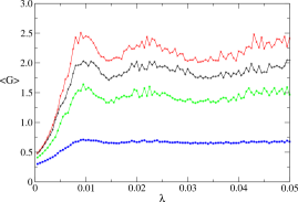
Figure 4: (Color online) Top panel: Average amplification $\left\langle G\right\rangle$ versus coupling $\lambda$ for a BA scale-free network and four values of the shape parameter: $m=0\ (+)$, $m=0.72\simeq m_{\max}\ (\times)$, $m=0.99$ (stars), and $m=1-10^{-6}$ (squares). Note that the first relative maximum of $\left\langle G\right\rangle$ occurs around $\lambda\approx 0.008$ for the four values of $m$ while the network has a maximal active hub having $136$ leaves. For this effective star-like network the theoretically predicted maximum occurs at $\lambda=\lambda_{\max,1}\approx 0.0074$. Bottom panel: Average amplification $\left\langle G\right\rangle$ versus shape parameter $m$ for a BA scale-free network and three values of the coupling: $\lambda=0.009\ \left(+\right)$, $\lambda=0.015\ (\times)$, and $\lambda=0.045$ (squares). Averaged degree $\left\langle\kappa\right\rangle=3$, $\gamma=2.7$, and the remaining fixed parameters are as in Fig. 3.

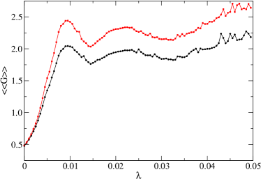
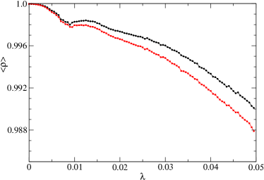
Figure 5: (Color online) Average of the average amplification over $10^{2}$ random realizations of the network connectivity $\left\langle\left\langle G\right\rangle\right\rangle\equiv\left\langle\max_{i}x_{i}/\tau\right\rangle$ for two values of the shape parameter ($m=0\$(circles) and $m=0.72\simeq m_{\max}\$(squares)) (top panel) and corresponding synchronization coefficient $\left\langle\rho\right\rangle$ [Eq. (2)] for $m=0$ and $m=0.72$ (bottom panel) versus coupling $\lambda$ for a BA scale-free network with $\left\langle\kappa\right\rangle=3,\gamma=2.7$. Other fixed parameters are as in Fig. 3.

Conclusion.$-$We have shown through the example of a network of overdamped bistable systems that maximizing the impulse transmitted by the periodic external signals strongly enhances topology-induced signal amplification in scale-free networks. We have analytically demonstrated that this resonant-like effect of the impulse is due to a correlative increase of the energy transmitted by the periodic signals as the impulse is increased, while it may be completely characterized in the simple model of a starlike network. Remarkably, our results indicate that varying the impulse does not significantly change the values of the coupling strength for which amplification is maximum, which means that the topology-induced amplification mechanism is robust against diversity in the uniform distributions of periodic external signals. Thus, the present findings provide a reliable criterion for the optimization of topology-induced amplification processes in scale-free networks by controlling the periodic external signals according to the impulse principle. This novel principle opens up new avenues for studying external-signal-induced amplification processes in complex networks, including, for example, control of chaos by weak periodic excitations [23], or optimization of signal transmission in neuronal networks [24,25] in which a cooperative effect with the underlying noise of the neural medium is expected under certain conditions.

P.J.M. and R.C. acknowledge financial support from the Ministerio de Economía y Competitividad (MINECO, Spain) through FIS2011-25167 and FIS2012-34902 projects, respectively. P.J.M. acknowledges financial support from the Comunidad de Aragón (DGA, Spain. Grupo FENOL) and European Social Funds. R.C. acknowledges financial support from the Junta de Extremadura (JEx, Spain) through project GR15146.

References

- (1) S. N. Dorogovtsev and J. F. F. Mendes, Evolution of networks: From biological nets to the Internet and WWW (Oxford Univ. Press, Oxford, 2003).
- (2) A.-L. Barabási and R. Albert, Science 286, 509 (1999).
- (3) R. Albert and A.-L. Barabási, Rev. Mod. Phys. 74, 47 (2002).
- (4) G. Caldarelli, Scale-free Networks: Complex Webs in Nature and Technology (Oxford Univ. Press, Oxford, 2007).
- (5) M. A. Serrano, D. Krioukov, and M. Boguñá, Phys. Rev. Lett. 100, 078701 (2008); Phys. Rev. Lett. 100, 199002(E) (2008).
- (6) V. Colizza, A. Flammini, M. A. Serrano, and A. Vespignani, Nat. Phys. 2, 110 (2006).
- (7) Y.-Y. Liu, J.-J. Slotine, and A.-L. Barabási, Nature 473, 167 (2011).
- (8) T. Nepusz and T. Vicsek, Nat. Phys. 8, 568 (2012).
- (9) E. López, S. V. Buldyrev, S. Havlin, and H. E. Stanley, Phys. Rev. Lett. 94, 248701 (2005).
- (10) L. Donetti, P. I. Hurtado, and M. A. Muñoz, Phys. Rev. Lett. 95, 188701 (2005).
- (11) C. Zhou and J. Kurths, Phys. Rev. Lett. 96, 164102 (2006).
- (12) Y. Chen, E. López, S. Havlin, and H. E. Stanley, Phys. Rev. Lett. 96, 068702 (2006).
- (13) H. Zhou and R. Lipowsky, Proc. Natl. Acad. Sci. U.S.A 102, 10052 (2005).
- (14) J. A. Acebrón, S. Lozano, and A. Arenas, Phys. Rev. Lett. 99, 128701 (2007); Phys. Rev. Lett. 99, 229902(E) (2007).
- (15) X. Liang, Z. Liu, and B. Li, Phys. Rev. E 80, 046102 (2009).
- (16) T. Kondo, Z. Liu, and T. Munakata, Phys. Rev. E 81, 041115 (2010).
- (17) J. Zhou, Y. Zhou, and Z. Liu, Phys. Rev. E 83, 046107 (2011).
- (18) P. Balenzuela, P. Rué, S. Boccaletti, and J. García-Ojalvo, New J. Phys. 16, 013036 (2014).
- (19) I. S. Gradshteyn and I. M. Ryzhik, Table of Integrals, Series, and Products (Academic Press, San Diego, 1980).
- (20) This measure is based on the root-mean-square of a -periodic function.
- (21) P. F. Byrd and M. D. Friedman, Handbook of Elliptic Integrals for Engineers and Scientists (Springer-Verlag, Berlin, 1971).
- (22) See Supplemental Material at xxx for an additional figure.
- (23) R. Chacón, Control of Homoclinic Chaos by Weak Periodic Perturbations (World Scientific, Singapore, 2005).
- (24) J. J. Torres, I. Elices, and J. Marro, PLoS ONE 10(3), e0121156 (2015).
- (25) S. J. Schiff, Neural Control Engineering (MIT Press, Cambridge, 2012).