Interplay between media and social influence
in the collective behavior of opinion dynamics

Abstract

Messages conveyed by media act as a major drive in shaping attitudes and inducing opinion shift. On the other hand, individuals are strongly affected by peers’ pressure while forming their own judgment. We solve a general model of opinion dynamics where individuals either hold one out of two alternative opinions or are undecided, and interact pairwise while exposed to an external influence. As media pressure increases, the system moves from pluralism to global consensus; four distinct classes of collective behavior emerge, crucially depending on the outcome of direct interactions among individuals holding opposite opinions. Observed nontrivial behaviors include hysteretic phenomena and resilience of minority opinions. Notably, consensus could be unachievable even when media and microscopic interactions are biased in favour of the same opinion: the unfavoured opinion might even gain the support of the majority.

I INTRODUCTION

Public opinion formation is a complex mechanism: people constantly process a huge amount of information to make their own judgment. Individuals form, reconsider and possibly change their opinions under a steady flow of news and a constant interchange with others. Social interactions have a strong effect on opinion formation Buchanan (2008): the pressure to conform to the opinion of others may in some cases even overcome empirical evidence Asch (1955) or undermine the wisdom of the crowd Lorenz et al. (2011). On the other hand media also play a central role: they can influence public knowledge, attitudes and behavior by choosing the slant of a particular news story, or just by selecting what to report. An intense activity has recently investigated macroscopic effects of these fundamental mechanisms exploiting the connection between opinion dynamics and simple non–equilibrium statistical physics models Castellano et al. (2009); Sen and Chakrabarti (2013). Media influence has been considered in the literature, in particular within the framework of cultural dynamics González-Avella et al. (2005, 2010); Peres and Fontanari (2011) and continuous opinion dynamics with heterogeneous confidence bounds Carletti et al. (2006); Vaz Martins et al. (2010); Quattrociocchi et al. (2014); Pineda and Buendía (2015). The fundamental case of binary opinions has received less attention for what concerns the role of media Bordogna and Albano (2007); Crokidakis (2012); Michard and Bouchaud (2005), although the similar case of proselytism by committed agents (zealots) has attracted considerable interest Mobilia (2003); Xie et al. (2011). The case of binary opinions is clearly relevant to yes/no questions, but not limited to that: when people are prompted with important questions that admit many possible answers their attitudes tend to be polarized, most people sharing one out of two opposite opinions Vallacher and Nowak (1994).

In this paper we address the problem of how people form their opinions based on the message they receive, both from traditional media and their social network, by studying a general class of opinion dynamics models. At any given time, each individual in the population is either supporting one of two alternative opinions or “undecided”. The possibility to be in a third state may have crucial effects in the case of a binary choice Vazquez et al. (2003); de la Lama et al. (2006); Castelló et al. (2006); Colaiori et al. (2015). Individuals are exposed to some external source of information biased towards one opinion (mainstream) and exchange information upon pairwise interaction: both factors may cause them to change their state. The undecided state accounts for individuals being uninterested, uninformed, or generally confused on the given issue. Carrying no opinion, they are assumed to have a passive role in the interactions. We account for the effect of media in the simplest possible way by assuming that people have some general tendency to conform to the media recommendation. On the other hand, we consider totally general rules for the interactions among pairs of agents. Our general model encompasses therefore a large class of specific models, each one identified by a given set of parameters defining the interaction rules. We study in mean-field this general model, determining the stationary solutions and their stability as a function of the external bias and of the parameters specifying pair interactions. We uncover the emergence of four distinct classes of collective behavior, characterized by different responses to the media exposure. Only two linear combinations of the parameters defining the general dynamics are relevant in determining which class a specific model belongs to. The results of numerical simulations, performed in systems with interaction patterns described by complex networks, support the general validity of the MF picture.

II GENERAL MODEL

We now define in detail the general model. Each agent can be in one of three states: holding opinion $A$, holding an opposing opinion $B$, or being undecided ($U$). Agents tend to conform to the media recommendation by adopting opinion $A$ at a constant rate $r$, independently of their current state, and interact pairwise at rate $f$. In the following we set $f=1$ to fix the time scale. Individuals in the same state are unaltered by their mutual interaction. In $A-U$($B-U$) interactions undecided agents may adopt, with given probability, their partner’s opinion, that they cannot alter: an agent holding opinion $A$ ($B$) has a probability $\varphi_{2}$ ($\gamma_{2}$) to convince the $U$ agent. We assume in general $\varphi_{2}\neq\gamma_{2}$, allowing for $A$ and $B$ to have unequal efficacy in persuading others. Interactions among agents holding opposite opinions ($A-B$) may have any outcome: each of the two agents may either keep her opinion, change it to match her partner’s opinion, or get confused and turn to the undecided state, in any combination. We indicate with $\left\{\alpha_{i}\right\}_{i=1}^{6}$ the probabilities of the six possible outcomes. Seven independent parameters fix the probabilities of each possible outcome for any interacting pair, as summarized in Table 1. While we consider for simplicity symmetric roles for the two interacting partners, our mean–field (MF) analysis holds more generally, also including models that assign distinct roles (e.g. speaker/listener) to the two partners. This more general case is discussed in Appendix A. Note that asymmetric models are always equivalent, in mean field, to their symmetrized version, the outcome of a symmetric interaction being the average result of asymmetric interactions with exchanged roles.

		$A,A$	$B,B$	$U,U$	$A,U$	$B,U$	$A,B$
$A-A$		$1$	$0$	$0$	$0$	$0$	$0$
$B-B$		$0$	$1$	$0$	$0$	$0$	$0$
$U-U$		$0$	$0$	$1$	$0$	$0$	$0$
$A-U$		$\varphi_{2}$	$0$	$0$	$1-\varphi_{2}$	$0$	$0$
$B-U$		$0$	$\gamma_{2}$	$0$	$0$	$1-\gamma_{2}$	$0$
$A-B$		$\alpha_{1}$	$\alpha_{2}$	$\alpha_{3}$	$\alpha_{4}$	$\alpha_{5}$	$\alpha_{6}$

Table 1: Each row in the table corresponds to an interaction, and each column to a possible outcome. Elements in the table indicate the probabilities of each possible outcome for the given interaction. In the last row $\sum_{i=1}^{6}\alpha_{i}=1$.

III MEAN FIELD EQUATIONS

The evolution of the system is described in MF by the dynamical equations for the density of agents in each state:

$$\!\!\left\{\begin{array}[]{lll}\!\!\dot{n}_{A}&\!\!=\!\!\!\!&r(1-n_{A})+2\varphi_{1}n_{A}n_{B}+2\varphi_{2}n_{A}(1-n_{A}-n_{B})\!\!\!\!\\ \!\!\dot{n}_{B}&\!\!=\!\!\!\!&-rn_{B}+2\gamma_{1}n_{A}n_{B}+2\gamma_{2}n_{B}(1-n_{A}-n_{B})\end{array}\!\!\!\right.$$ (1)

where $n_{A}$ ($n_{B}$) denote the density of agents in the $A$ ($B$) state, and $\varphi_{1}=\alpha_{1}-\alpha_{2}-\alpha_{3}-\alpha_{5}$, $\gamma_{1}=-\alpha_{1}+\alpha_{2}-\alpha_{3}-\alpha_{4}$. The density $n_{U}$ of undecided agents is obtained by normalization: $n_{U}=1-n_{A}-n_{B}$. The densities must belong to the physical region of the plane $(n_{A},n_{B})$, defined by the three constraints $n_{A}\geq 0$, $n_{B}\geq 0$, $n_{A}+n_{B}\leq 1$. The coefficients $\alpha_{i}$ appear in Eq. (1) only in two linear combinations $\varphi_{1}$ and $\gamma_{1}$ that represent the total average variation in $A$ ($B$) states due to an $A-B$ interaction. This reduces the number of effective parameters from seven to four plus the external bias $r$, acting as a control parameter. The parameters $\varphi_{1}$ and $\gamma_{1}$ are bounded by $-1\leq\gamma_{1}\leq 1$, $-1\leq\varphi_{1}\leq 1$, $\gamma_{1}+\varphi_{1}\leq 0$ (the sum $\gamma_{1}+\varphi_{1}$ is minus the average net production of undecided in an $A-B$ interaction, that has to be non negative). Stationary solutions of Eq. (1) are the intersections of the two conic sections:

$$\!\left\{\begin{array}[]{lr}\!\!n_{A}\left[(\varphi_{2}-\varphi_{1})n_{B}+\varphi_{2}n_{A}-\varphi_{2}+r/2\right]=r/2&\,\,\,{\cal C}_{1}\!\!\\ \!\!n_{B}\left[(\gamma_{1}-\gamma_{2})n_{A}-\gamma_{2}n_{B}+\gamma_{2}-r/2\right]=0&\,\,\,{\cal C}_{2}\!\!\end{array}\!\!\right.$$ (2)

The curve ${\cal C}_{1}$ is an hyperbola. One of its asymptotes is the axis $n_{A}=0$, so that only the upper branch ${\cal C}_{1}^{+}$ ($n_{A}>0$) is physically relevant. The curve ${\cal C}_{2}$ factorizes into the product of two lines, ${\cal R}_{1}$, and ${\cal R}_{2}$. The line ${\cal R}_{1}$ ($n_{B}=0$) always intercepts ${\cal C}_{1}^{+}$ in $P_{1}\equiv[n_{B}=0,n_{A}=1]$, corresponding to the absorbing state of total consensus on opinion $A$. Depending on the parameters, ${\cal R}_{2}$ may intersect ${\cal C}_{1}^{+}$ in one, two (possibly coincident) points, either inside or outside the physical region, or none. Varying the control parameter $r$, different fixed points arise and move entering and exiting the physical region. Their flow and stability determine the collective response to the external bias.

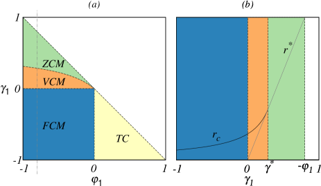
Figure 1: (color online)(a) Phase diagram in the ($\varphi_{1}$, $\gamma_{1}$) plane. The curve $\gamma_{1}^{*}$ separating regions $VCM$ and $ZCM$ depends on $\varphi_{2}$ and $\gamma_{2}$ (in the figure $\varphi_{2}=0.1$ and $\gamma_{2}=0.5$). (b) Plot of $r_{c}$ (saddle–node bifurcation curve) and $r^{*}$ (transcritical bifurcation line) as functions of $\gamma_{1}$, and for $\varphi_{1}=-0.8$.

By studying them we find the phase-diagram represented in Fig. 1(a), which constitutes the main result of our paper. As a function of the external bias $r$ there are four distinct classes of collective behavior, associated with different regions of the parameter space. Notably, the emergent behavior is essentially ruled by only two of the parameters, $\varphi_{1}$ and $\gamma_{1}$. In the next section we discuss the qualitative features of each class, referring to Appendix B for analytical details on the derivation of the phase diagram.

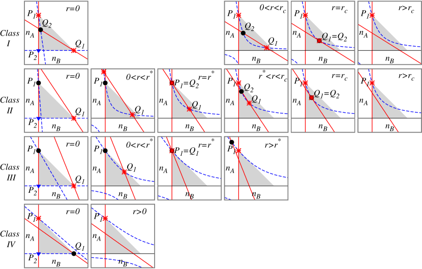
Figure 2: Plots of isoclines and fixed points for each class of models and each range of $r$. Red solid lines are ${\cal R}_{1}$ and ${\cal R}_{2}$, the blu dashed curve is the hyperbola ${\cal C}_{1}$. Red stars denote stable fixed points, black circles denote saddle points, blue triangles denote repulsive fixed points. The shaded triangle represents the physical region $n_{A}\geq 0$, $n_{B}\geq 0$, $n_{A}+n_{B}\leq 1$. Plots in the first row correspond to $\varphi_{1}=-0.6$, $\varphi_{2}=0.1$, $\gamma_{1}=-0.3$, $\gamma_{2}=0.5$, and $r=0$, $r=r_{c}/2$, $r=r_{c}$, $r=r_{c}+0.05$. Plots in the second row correspond to $\varphi_{1}=-0.6$, $\varphi_{2}=0.05$, $\gamma_{1}=0.1$, $\gamma_{2}=0.3$, and $r=0$, $r=r^{*}/2=\gamma_{1}$, $r=r^{*}=\gamma_{1}$, $r=0.2r^{*}+0.8r_{c}$, $r=r_{c}$, $r=r_{c}+0.05$. Plots in the third row correspond to $\varphi_{1}=-0.5$, $\varphi_{2}=0.7$, $\gamma_{1}=0.3$, $\gamma_{2}=0.5$, and $r=0$, $r=r^{*}/2=\gamma_{1}$, $r=r^{*}=\gamma_{1}$, $r=r^{*}+0.1$. Plots in the fourth row correspond to $\varphi_{1}=0.1$, $\varphi_{2}=0.7$, $\gamma_{1}=-0.2$, $\gamma_{2}=0.5$, and $r=0$, $r=0.2$.

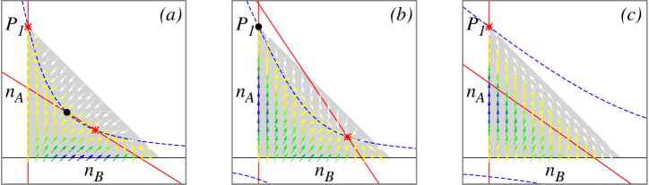
Figure 3: (color online) Phase portrait relative to Eq. (1): flows in the vector field indicate the time evolution of the system. Fixed points are the intersections between either of the two lines ${\cal R}_{1}$, ${\cal R}_{2}$ (red solid lines), and the curve ${\cal C}_{1}$ (blue dashed line). Black circles are saddle points, red stars are attractive fixed points. (a) $FCM$ model in the region $r<r_{c}$ ($\varphi_{1}=-0.6$, $\varphi_{2}=0.1$, $\gamma_{1}=-0.3$, $\gamma_{2}=0.5$, $r=0.1$); (b) $VCM$ model in the range $r<r^{*}$ ($\varphi_{1}=-0.6,\varphi_{2}=0.4$, $\gamma_{1}=0.1$, $\gamma_{2}=0.3$, $r=0.13$); (c) $TC$ model ($\varphi_{1}=0.1$, $\varphi_{2}=0.7$, $\gamma_{1}=-0.2$, $\gamma_{2}=0.5$, $r=0.2$). The flow is qualitatively similar to (a) for $VCM$ models with $r^{*}<r<r_{c}$, to (b) for $ZCM$ models with $r<r_{c}$, to (c) for any class of models above $r_{c}$. See Appendix B for further details.

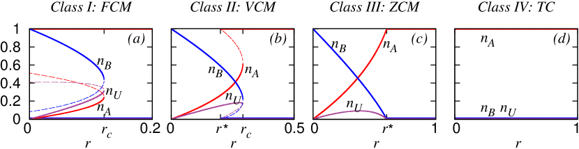
Figure 4: (color online) Theoretical results for the densities of agents for realizations of each of the four classes of models: (a) Class I model (FCM) ($\varphi_{1}=-0.5$, $\varphi_{2}=0.1$, $\gamma_{1}=-0.4$, and $\gamma_{2}=0.5$), (b)Class II model (VCM) ($\varphi_{1}=-0.5$, $\varphi_{2}=0.1$, $\gamma_{1}=0.1$, and $\gamma_{2}=0.5$), (c)Class III model (ZCM) ($\varphi_{1}=-0.5$, $\varphi_{2}=0.1$, $\gamma_{1}=0.3$, and $\gamma_{2}=0.5$), (d)Class IV model (TC) ($\varphi_{1}=0.3$, $\varphi_{2}=0.1$, $\gamma_{1}=-0.5$, and $\gamma_{2}=0.5$). Solid (dashed) lines represent stable (unstable) lines.

Fig. 2 represents the shapes of the curves in Eq. (2), allowing to understand the existence and positions of stationary solutions. Fig. 3 provides information on flows and the stability of solutions. Fig. 4 depicts the resulting behavior of the densities of agents in the different states as a function of $r$.

IV CLASSES OF COLLECTIVE BEHAVIOR

IV.1 Class I: Finite Critical Mass (FCM) Models

When $\varphi_{1}<0$, $\gamma_{1}\leq 0$, i.e. in models where $A-B$ interactions produce on average an increase in undecided individuals with no net gain in $A$ nor in $B$ states, the system undergoes a first order transition at a finite value $r=r_{c}$ of the external bias (see Fig. 2, first row). For large enough $r$ $P_{1}$ is the only fixed point and the system flows into the absorbing state of total consensus on opinion $A$ for any initial condition. At $r=r_{c}$ the system undergoes a saddle–node bifurcation Strogatz (2001): two additional coinciding fixed points appear. As $r$ is decreased below $r_{c}$ they split (one, with larger $n_{B}$, stable, the other unstable, see Fig. 3(a)). In the nontrivial stable fixed point the two opinions $A$ and $B$ coexist in the population, together with a fraction of undecided (we call this state “pluralism”), see Fig. 4(a). The initial conditions determine whether the pluralistic state ($n_{B}>0$) or the consensus state ($n_{A}=1$) is asymptotically reached. The value of $n_{B}$ at the unstable fixed point stays finite in the limit $r\rightarrow 0$ (see Fig. 2, first row), implying that a finite “critical mass” Dodds and Watts (2004) of dissenters is always needed to reach the pluralistic state, no matter how small is the external bias.

IV.2 Class II: Vanishing Critical Mass (VCM) Models

This class is identified by $\varphi_{1}<0$, $0<\gamma_{1}<\gamma_{1}^{*}$, and corresponds to models where $A-B$ interactions cause on average a small increase of $B$ states at the expense of $A$ states. As in Class I, lowering $r$ below $r_{c}$ the system undergoes a first order transition separating a regime ($r>r_{c}$), where consensus on opinion $A$ is the only stable state from a regime ($r<r_{c}$) where a stable and an unstable additional fixed points appear through a saddle–node bifurcation (Fig. 2, second row). However, in this case, further reducing $r$, the unstable fixed point collides with the point $P_{1}$ (consensus on $A$) at a finite value $r^{*}$ ($0<r^{*}<r_{c}$), and then exits the physical region. This is a transcritical bifurcation Strogatz (2001): when the two fixed points cross each other, they exchange stability (Fig. 3(b)); $P_{1}$ becomes unstable, so that below $r^{*}$ the system, unless started with $n_{B}\equiv 0$, always flows to the pluralistic state (Fig. 4(b)). The initial presence of even a few dissenters suffices for opinion $B$ to survive. The curve $\gamma_{1}^{*}(\varphi_{1})=\varphi_{1}\gamma_{2}/(\varphi_{1}-\varphi_{2}-\gamma_{2})$ separating Class II and III depends on the parameters $\varphi_{2}$ and $\gamma_{2}$ (see Appendix B). The transcritical bifurcation line is $r=r^{*}=2\gamma_{1}$ (see Appendix B), and always lies below the saddle–node bifurcation line (see Fig. 1(b)).

IV.3 Class III: Zero Critical Mass (ZCM) Models

When $\varphi_{1}<0$, $\gamma_{1}\geq\gamma_{1}^{*}$, corresponding to models where $A-B$ interactions give an increase of undecided and a large increase in $B$ at the expense of $A$, the system undergoes at $r=r^{*}=2\gamma_{1}$ a continuous transition (transcritical bifurcation) between total consensus on opinion $A$ ($r>r^{*}$) and pluralism ($r<r^{*}$), see Fig. 2, third row, and Fig. 4(c). Initial conditions do not play any role.

IV.4 Class IV: Total Consensus (TC) Models

The region $\varphi_{1}\geq 0$ corresponds to models where $A-B$ interactions result in a net increase of individuals holding opinion $A$. The behavior is trivial (see Fig. 3, fourth row): irrespectively of the value of all other parameters, for any initial condition, and no matter how small the external forcing is, the system always converges to the consensus state ($P_{1}$) (see Fig. 3(c) and 4(d)).

V BEYOND MEAN–FIELD

Before discussing the analytical results obtained in the previous section within MF and examining some of their consequences we test their validity beyond MF by numerical simulations on synthetic and real–word networks. The simulations are performed on four microscopic dynamical models, each belonging to one of the universality classes derived above.

The single event of the dynamics occurs as follows not (a). We select randomly a node $i$ (speaker) and, with probability $r/(1+r)$, we set his state to $A$, as effect of the external bias. Instead, with complementary probability $1/(1+r)$ an interaction process takes place: we select a listener $j$ among the neighbors of $i$, and modify the state of the pair ($i$, $j$) according to Table 2 in Appendix B with probabilities $\psi_{2}=\omega_{2}=\varphi_{2}$, $\delta_{2}=\epsilon_{2}=\gamma_{2}$ and each $\lambda_{i}=\mu_{i}=\alpha_{i}$ for any $i$. Each single event occurs during a temporal interval $1/N$ (where $N$ is the total number of nodes in the network), so that $N$ updates are attempted in a time unit. Starting from the initial configuration, for each value of $r$ we let the system evolve during 5000 time steps to reach the stationary configuration and determine the densities $n_{A}$, $n_{B}$ and $n_{U}$ by performing averages over 5000 additional time steps. In order to characterize the possible presence of discontinuous phase transitions and the associated hystereric effects, for each set of data we consider two different initial conditions: either all nodes in state $B$ ($n_{B}=1$), or all nodes in state A except for a very small fraction of nodes in state $B$ ($n_{A}=0.99$, $n_{B}=0.01$). We always keep the values $\varphi_{2}=0.1$ and $\gamma_{2}=0.5$ fixed and vary $\gamma_{1}$ and $\varphi_{1}$ in order to encompass all four quantitatively distinct behaviors found in the analytic approach.

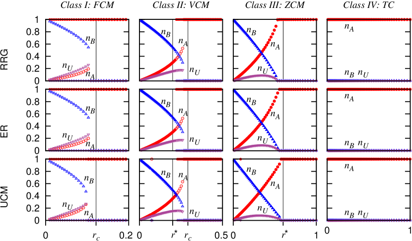
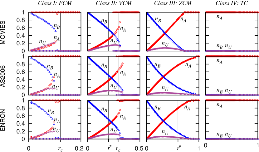
Figure 5: (color online) Stationary densities of nodes in the various states as a function of the external bias $r$ for three types of synthetic networks and three real networks described in the text. Empty (filled) symbols refer to the $n_{B}=1$, $n_{A}=0$ ($n_{B}=0.01$, $n_{A}=0.99$) initial condition. Red circles, blue upward triangles, violet downward triangles represent $n_{A}$, $n_{B}$, and $n_{U}$, respectively. The values of $\varphi_{2}=0.1$ and $\gamma_{2}=0.5$ are fixed. From left to right the values of the pair $(\varphi_{1},\gamma_{1})$ are $(-0.5,-0.4)$, $(-0.5,0.1)$, $(-0.5,0.3)$ and $(0.1,-0.5)$, corresponding respectively to classes I, II, III and IV according to the MF classification scheme. Notice that in class I, $r^{*}\approx 1$ for AS2006, but since $r$ is a rate there is still an extended consensus region for $r>r^{*}$.

V.1 Simulations on synthetic networks

In Fig. 5 (upper panel) we plot the stationary value of the densities as a function of $r$ when the interaction pattern is given by three synthetic networks of size $N=20000$: a Random Regular Graph (RRG) where each node has 10 neighbors; an Erdös-Rényi(ER) graph of average degree 10; a network built using the Uncorrelated Configuration Model (UCM) with minimum degree $3$ and degree distribution decaying as $k^{-2.5}$. For all these cases, predictions are very well matched by numerical simulations.

V.2 Simulations on real networks

A tougher test of the MF results is provided by simulations performed on real–world networks, incorporating additional topological features such as clustering and correlations. In Fig. 5 (lower panel) we report results for: a network of size $N=81860$ representing movie actor collaborations obtained from the Internet Movie Database (MOVIES) (average degree $\langle k\rangle=89.53$, fluctuations $\langle k^{2}\rangle/\langle k\rangle=594.91$); a network of size $N=24608$ representing connections of Internet Autonomous Systems in 2006 (AS2006) (average degree $\langle k\rangle=4.05$, fluctuations $\langle k^{2}\rangle/\langle k\rangle=259.94$) ; the largest connected component (size $N=33696$) of the Enron email exchange network (ENRON) (average degree $\langle k\rangle=10.02$, fluctuations $\langle k^{2}\rangle/\langle k\rangle=140.07$) Leskovec and Krevl (2014).

Also in these cases numerical simulations agree well with the outcome of the MF approach: the behavior in each of the classes qualitatively reproduces the analytical predictions, with only (expected) variations in the position of transition points. The only variation in this respect concerns class I. In this case it turns out that for very small values of the rate $r$ the state with overwhelming majority of $B$ is dynamically reached even starting from $n_{B}$ as low as $0.01$, at odds with the MF prediction.

VI DISCUSSION AND CONCLUSIONS

We finally discuss some interesting and nontrivial consequences that follow from the classification scheme derived within the MF approach.

Although the parameters regulating the interactions with undecided agents have a marginal role in determining the collective behavior, the presence itself of the $U$ state is crucial in several respects. In the absence of the third, undecided state, the system would either converge to total consensus on opinion $A$ (Class IV)– when asymmetric interactions favor $A$, or exhibit a continuous transition between consensus and pluralism (Class III) – when asymmetric interactions favor $B$ Colaiori et al. (2015).

Several models in the literature that allow for a third state require $U$ to be a necessary intermediate step when changing opinion Marvel et al. (2012); Castelló et al. (2006). Our results imply that such systems undergo a discontinuous transition by varying the media exposure: $U$ being a necessary intermediate step requires $\alpha_{1}=\alpha_{2}=0$, giving $\varphi_{1}\leq 0$, $\gamma_{1}\leq 0$; therefore these models always fall in Class I. The condition for a model to be in Class I is however more general, only excluding average gain of $A$ or $B$ in $A-B$ interactions.

Within our framework consensus is always achieved, whatever the interactions, for strong enough media exposure. Then a natural question arises: is consensus stable upon removal of the media pressure? The answer to this question is different for different classes. In FCM class, once the consensus is reached, it is kept also when the media exposure is removed. In ZCM class dissenters nucleate as soon as the media exposure is lowered below the threshold needed to reach consensus ($r<r_{c}$). VCM class shows interesting hysteretic behavior: once consensus is reached with a sufficiently high media exposure ($r>r_{c}$), it is kept when lowering the media pressure that however cannot be completely turned off: below $r^{*}$ consensus on opinion $A$ becomes unstable and any infinitesimal perturbation causes an abrupt transition to a pluralistic state.

Finally, a markedly counter–intuitive fact emerges from our analysis, namely the possibility for $B$ states to survive, and even become the majority, also when both the external forcing and the interaction rules are biased against them. Examples are systems in the FCM class that have $\gamma_{1}<\varphi_{1}$ (more $B$ than $A$ states are lost in $A-B$ interactions), and $\varphi_{2}>\gamma_{2}$ (individuals in $A$ state have more success than those in $B$ state in convincing undecided individuals). In this case, both the external pressure and the rules of peer interactions favor $A$, yet for small values of $r$ and suitable initial conditions a stationary state with $n_{B}>0$ is reached. Here the role of the third state is crucial: although the peer interaction rules are asymmetric in favor of the $A$ state, the rate at which they occur allows the $B$ state to be favored on average not (b).

Analytical predictions derived in MF are well matched by numerical simulations performed both on synthetic and real networks: the collective behavior for sample models in each of the four classes qualitatively reproduces the analytical predictions. The only observed deviation from MF concerns models in class I on some real topologies. In this case, for very small values of the rate $r$, even when the initial state has $n_{B}$ as low as $0.01$, the state with overwhelming majority of $B$ is dynamically reached while MF would predict that total consensus is achieved for suitably small values of $n_{B}$ in the initial condition. This could reflect topological features such as clustering or correlations present in the networks.

In conclusion, we have shown how four qualitatively distinct kinds of collective dynamics emerge from the interplay between mass media and social influence, and categorized a very extensive set of opinion dynamics models accordingly. The four classes are non–degenerate in the sense that they occupy a finite region of the parameter space. The macroscopic behavior is independent of many details and essentially determined by the outcome of direct interactions among agents holding opposite opinions. While the existence of undecided individuals is crucial, the parameters that define their interactions only participate in locating the fixed points and the line separating classes II and III. Nontrivial effects, including dependence on initial conditions and history–dependence are observed.

The existence of a pluralistic state is desirable in many circumstances, but it could lead to a deadlock when unanimous agreement is required. Assuming very general interactions among peers we give conditions for a pluralistic state to exist and survive an external pressure under the schematic hypothesis that people generally tend to conform to the message conveyed by the media. An interesting direction for further research would include within our framework more sophisticated descriptions of how public opinion is shaped by media, such as the “two–step flow” model Katz and Lazarsfeld (1955); Lazarsfeld et al. (1968) accounting for the role of opinion leaders or as in more recent theories Dodds and Watts (2007) focusing on information cascades triggered by a critical mass of easily influenced individuals.

Appendix A: Generalization to models with asymmetric roles

In the main text we considered generic rules for the peer interactions, but we assumed symmetric roles for the two interacting partners. However we mentioned that our mean–field analysis holds more generally, including cases where the interaction partners have distinct roles (e.g. speaker/listener), as often considered in the literature. We here introduce a further generalization of our model that allows for asymmetric roles, for which all the results derived in mean–field still hold. This consists in replacing the peer interactions with those in Table 2.

S      L		$\,AA\,$	$\,BB\,$	$\,UU\,$	$AU$	$UA$	$BU$	$UB$	$\,AB\,$	$\,BA\,$
$A-A$		$1$	$0$	$0$	$0$	$0$	$0$	$0$	$0$	$0$
$B-B$		$0$	$1$	$0$	$0$	$0$	$0$	$0$	$0$	$0$
$U-U$		$0$	$0$	$1$	$0$	$0$	$0$	$0$	$0$	$0$
$A-U$		$\psi_{2}$	$0$	$0$	$1\!-\!\psi_{2}$	$0$	$0$	$0$	$0$	$0$
$U-A$		$\omega_{2}$	$0$	$0$	$0$	$1\!-\!\omega_{2}$	$0$	$0$	$0$	$0$
$B-U$		$0$	$\delta_{2}$	$0$	$0$	$0$	$1\!-\!\delta_{2}$	$0$	$0$	$0$
$U-B$		$0$	$\epsilon_{2}$	$0$	$0$	$0$	$0$	$1\!-\!\epsilon_{2}$	$0$	$0$
$A-B$		$\lambda_{1}$	$\lambda_{2}$	$\lambda_{3}$	$\lambda_{4}$	$\lambda_{5}$	$\lambda_{6}$	$\lambda_{7}$	$\lambda_{8}$	$\lambda_{9}$
$B-A$		$\mu_{1}$	$\mu_{2}$	$\mu_{3}$	$\mu_{4}$	$\mu_{5}$	$\mu_{6}$	$\mu_{7}$	$\mu_{8}$	$\mu_{9}$

Table 2: Each row in the table corresponds to an interaction between a speaker, leading the conversation, and a listener, and each column to a possible outcome, given by an ordered couple (speaker,listener). Elements in the table indicate the probabilities of each possible outcome for the given interaction. In the last two rows $\sum_{i=1}^{9}\lambda_{i}=1$, and $\sum_{i=1}^{9}\mu_{i}=1$.

The very complicated system defined by the interactions in Table 2 is still described in mean–field by Eqs. (1) once we properly define the coefficients in Eqs. (1) as functions of the 22 parameters in Table 2. In particular, we have $\varphi_{2}=(\psi_{2}+\omega_{2})/2$, $\gamma_{2}=(\delta_{2}+\epsilon_{2})/2$, $\varphi_{1}=(\lambda_{1}+\mu_{1}-\lambda_{2}-\mu_{2}-\lambda_{3}-\mu_{3}-\lambda_{5}-\mu_{5})/2$, and $\gamma_{1}=(-\lambda_{1}-\mu_{1}+\lambda_{2}+\mu_{2}-\lambda_{3}-\mu_{3}-\lambda_{4}-\mu_{4})/2$. We could also allow agents to exchange their state in an $A-U$ interaction giving $UA$ as outcome (and similarly for $U-A$, $B-U$, and $U-B$ interactions): our analysis and results would still hold, however this goes beyond our interpretation of agents in state $U$ as having no opinion or information to convey.

We note that the irrelevance of the distinction between roles holds in mean–field in full generality: a model allowing for asymmetric roles is always equivalent at the mean–field level to its symmetrized version, the outcome of an interaction in the symmetrized model being defined as the average result of two asymmetric interactions with exchanged roles.

Appendix B: Analytical details of the mean–field analysis

We present here a detailed derivation of the phase diagram discussed in the main text. The general model is described by Eqs. (1) for the densities of agents in $A$ and $B$ states, the density $n_{U}$ of undecided agents being $n_{U}=1-n_{A}-n_{B}$. Stationary solutions are given by the intersections of the two conic sections ${\cal C}_{1}$ and ${\cal C}_{2}$ in Eqs. (2).

Excluding the cases $\varphi_{2}=0$ and $\gamma_{2}=0$ that will be discussed separately, and defining $\varphi=(\varphi_{1}-\varphi_{2})/\varphi_{2}$ and $\gamma=(\gamma_{1}-\gamma_{2})/\gamma_{2}$ we rewrite Eqs. (2) as:

$$\!\left\{\begin{array}[]{lr}\!\!n_{A}\left(n_{A}-\varphi n_{B}+r/(2\varphi_{2})-1\right)=r/(2\varphi_{2})&\,\,\,{\cal C}_{1}\!\!\\ \!\!n_{B}\left(\gamma n_{A}-n_{B}+1-r/(2\gamma_{2})\right)=0&\,\,\,{\cal C}_{2}\!\!.\end{array}\!\!\right.$$ (3)

Since physically relevant solutions must belong to the domain $n_{A}\geq 0$, $n_{B}\geq 0$, $n_{A}+n_{B}\leq 1$, only the upper branch ${\cal C}_{1}^{+}$ of the hyperbola ${\cal C}_{1}$ matters:

$$n_{A}=\left(\varphi n_{B}+1-r/(2\varphi_{2})+\sqrt{\Delta_{1}}\right)/2\,\,\,\,\,\,{\cal C}_{1}^{+}\!\!,$$ (4)

where $\Delta_{1}=(\varphi n_{B}+1-r/(2\varphi_{2}))^{2}+2r/\varphi_{2}$. The conic section ${\cal C}_{2}$ is degenerate and factorizes in the two lines:

$$\begin{array}[]{lr}n_{B}=0&\,\,{\cal R}_{1}\\ n_{A}=n_{B}/\gamma+(r/(2\gamma_{2})-1)/\gamma&\,\,{\cal R}_{2}\!.\end{array}$$ (5)

${\cal C}_{1}$ and ${\cal R}_{1}$ always have two intersections: $P_{1}=[n_{B}=0,n_{A}=1]$, corresponding to total consensus on opinion $A$, and $P_{2}=[n_{B}=0,n_{A}=-r/(2\varphi_{2})]$, that is always outside of the the physical region. Therefore, the parameter dependence of the system that differentiates the four classes of behavior is entirely determined by possible additional solutions given by the intersections between ${\cal C}_{1}^{+}$ and ${\cal R}_{2}$.

The slope of the line ${\cal R}_{2}$ is $m_{{\cal R}_{2}}=1/\gamma$, independent of $r$, and fixed once we fix the model parameters. For large $r$ the intercept of ${\cal R}_{2}$ tends to either $\pm\infty$, depending on the sign of $\gamma$. This implies that, independent on the value of the parameters, full consensus on $A$ (the point $P_{1}$) is the only stationary solution for large $r$. As $r$ decreases, ${\cal R}_{2}$ translates towards the physical region, while ${\cal C}_{1}^{+}$ becomes more and more squeezed towards its asymptotes $n_{A}=0$, and $n_{A}=\varphi n_{B}-r/(2\varphi_{2})+1$ and degenerates into their product as $r\rightarrow 0$. In order to understand if and when other solutions appear, it is useful to analyze first the behavior in the limit of no bias.

Limit of no bias ($r\rightarrow 0$)

We now consider the limit of no bias ($r\rightarrow 0$). In such a limit ${\cal R}_{2}$ has equation $n_{A}=n_{B}/\gamma-1/\gamma$, and ${\cal C}_{1}$ degenerates into the product of its asymptotes $n_{A}=0$ and $n_{A}=\varphi n_{B}+1$:

$$\left\{\begin{array}[]{lr}n_{A}(n_{A}-\varphi n_{B}-1)=0&\,\,\,{\cal C}_{1}\!\!\\ n_{B}(\gamma n_{A}-n_{B}+1)=0&\,\,\,{\cal C}_{2}\!\!.\end{array}\right..$$ (6)

In this case ${\cal C}_{2}$ and ${\cal C}_{1}$ have four intersections: $P_{1}=[n_{B}=0,n_{A}=1]$, $P_{2}=[n_{B}=0,n_{A}=0]$ (intersections of ${\cal R}_{1}$ with the degenerate hyperbola), and $Q_{1}=[n_{B}=1,n_{A}=0]$, $Q_{2}=[n_{B}^{*},n_{A}^{*}]$ (intersections of ${\cal R}_{2}$ with the degenerate hyperbola), where

$$\begin{array}[]{l}n_{A}^{*}=(1+\varphi)/(1-\varphi\gamma)\\ n_{B}^{*}=(1+\gamma)/(1-\varphi\gamma)\,.\end{array}$$ (7)

$Q_{2}$ is the only fixed point that depends on the model parameters: it falls inside the physical region for $\varphi_{1}\leq 0$, $\gamma_{1}\leq 0$, and outside in all other cases. This can be proven by noting that the conditions $\varphi_{1}\leq 0$, $\gamma_{1}\leq 0$ translate into $\varphi\leq-1$, and $\gamma\leq-1$, which also give $\varphi\gamma\geq 1$. Therefore $(1+\varphi)$, $(1+\gamma)$ and $(1-\varphi\gamma)$ are all negative, implying $n_{A}^{*}\geq 0$, $n_{B}^{*}\geq 0$. Moreover $n_{A}^{*}+n_{B}^{*}=(2+\varphi+\gamma)/(1-\varphi\gamma)=1+(1+\varphi+\gamma+\varphi\gamma)/(1-\varphi\gamma)=1+(1+\varphi)(1+\gamma)/(1-\varphi\gamma)\leq 1$. In the region $\varphi_{1}>0$, $\gamma_{1}<0$, $n_{A}^{*}$ and $n_{B}^{*}$ have opposite sign, therefore one of the two has to be negative, and the point $Q_{2}$ falls outside the physical region. The same reasoning holds for $\varphi_{1}<0$, $\gamma_{1}>0$. Stability analysis trivially gives that the fixed point $P_{2}$ (with eigenvalues $2\varphi_{2}$ and $2\gamma_{2}$) is always repulsive. The fixed point $P_{1}$ (with eigenvalues $2\gamma_{1}$ and $-2\varphi_{2}$) is attractive for $\gamma_{1}<0$ and a saddle point for $\gamma_{1}>0$, while the fixed point $Q_{1}$ (with eigenvalues $-2\gamma_{2}$ and $2\varphi_{1}$) is attractive for $\varphi_{1}<0$ and a saddle point for $\varphi_{1}>0$. When physically relevant (for $\varphi_{1}\leq 0$, $\gamma_{1}\leq 0$), the fixed point $Q_{2}$ is always a saddle point. These results are summarized in the first column of Fig. 2.

Case $\varphi_{1}\geq 0$

For $\varphi_{1}\geq 0$ the upper branch ${\cal C}_{1}^{+}$ of the hyperbola only crosses the physical region in the point $P_{1}$, therefore in that case the status of total consensus on opinion $A$ is the only fixed point (see Fig. 2, fourth row). This can be proven by looking at the slope of the tangent ${\cal T}$ to ${\cal C}_{1}^{+}$ in $P_{1}$. From Eq. (2) the equation of ${\cal T}$ is

$$n_{A}=\varphi/(1+r/(2\varphi_{2}))n_{B}+1\,\,\,\,\,\,\,\,\,\,\,{\cal T}.$$ (8)

${\cal C}_{1}^{+}$ enters the physical region only when the angular coefficient $m_{{\cal T}}=\varphi/(1+r/(2\varphi_{2}))$ of ${\cal T}$ is $m_{{\cal T}}<-1$, but this condition is never met for $\varphi_{1}\geq 0$. This proves that in the region $\varphi_{1}\geq 0$ of the parameter space corresponding to Class IV models, no transition occurs (see the phase diagram shown in Fig. (1(a))). In what follows we therefore restrict our analysis to the case $\varphi_{1}<0$ ($\varphi<-1$).

Saddle–node bifurcation line

For $\varphi_{1}<0$ it is always $m_{{\cal T}}<-1$, therefore ${\cal C}_{1}^{+}$ goes through the physical region. We want to determine under what conditions a saddle–node bifurcation occurs, i.e. two additional physical solutions (interceptions of ${{\cal C}_{1}}$ and ${{\cal R}_{2}}$) appear for a critical value of the bias $r=r_{c}$. In general when a straight line crosses an hyperbola, the two intersections either lie on the same branch or one on each branch, depending on the slope of the straight line relative to the slope of the asymptotes. In our case, for any $r$ the slopes of the hyperbola asymptotes are $0$ and $\varphi$, while the slope of ${{\cal R}_{2}}$ is $1/\gamma$. Therefore we must distinguish the two following cases:
$(a)$ For $\varphi<1/\gamma<0$ the line ${\cal R}_{2}$ either intercepts the same branch of the hyperbola in two points $Q_{1}$ and $Q_{2}$ (possibly coincident), or it has no intersections at all.
$(b)$ For $1/\gamma<\varphi$ or $1/\gamma>0$ the line ${\cal R}_{2}$ always intercepts the hyperbola in two points, one on each branch.

The equation for the intercepts is obtained from Eq. (3):

$$\Gamma n_{A}^{2}-n_{A}B(r)+r/(2\varphi_{2})=0$$ (9)

where $B(r)=r/(2\varphi_{2})(1+\varphi\varphi_{2}/\gamma_{2})-(1+\varphi)$ and $\Gamma=\varphi\gamma-1$. If $\Gamma<0$ (case $(b)$) the discriminant $\Delta=B(r)^{2}-4\Gamma r/(2\varphi_{2})$ is positive for any value of $r$. In this case there is no saddle–node bifurcation. If instead $\Gamma>0$ (case $(a)$) $\Delta$ is positive (i.e. there are two intersections) for $r\leq r_{c}$ given by the equation

$$r_{c}^{2}A^{2}-4r_{c}\varphi_{2}(A(1+\varphi)+2\Gamma)+4\varphi_{2}^{2}(1+\varphi)^{2}=0$$ (10)

where $A=1+\varphi\varphi_{2}/\gamma_{2}$.

At $r=r_{c}$, the two solutions $Q_{1}$ and $Q_{2}$ of Eq. (9) coincide in $n_{A}=B(r_{c})/2\Gamma=\sqrt{r_{c}/(2\varphi_{2}\Gamma)}$. For the saddle–node bifurcation to have a physical relevance the two coincident solutions $Q_{1}=Q_{2}$ must appear inside the physical region. Requiring $n_{A}<1$ implies $r_{c}/(2\varphi_{2})<\Gamma$. Solving Eq. (10) for $r_{c}$ and replacing its value in the previous inequality gives, after some algebra, the condition $\gamma_{1}<\gamma_{1}^{*}$, where

$$\gamma_{1}^{*}=\varphi_{1}\gamma_{2}/(\varphi_{1}-\varphi_{2}\gamma_{2})\,.$$ (11)

Therefore a discontinuous physical transition always occurs for $\varphi_{1}<0$ and $\gamma_{1}<\gamma_{1}^{*}$. For $\gamma_{1}>\gamma_{1}^{*}$ the two intersections appear instead outside the physical region. The saddle–node bifurcation line is shown in Fig. (1(b)), where $r_{c}$ is plotted versus $\gamma_{1}$ for fixed negative $\varphi_{1}$. As discussed in the folowing, when $r$ is further lowered, the two intersections might exit the physical region.

Transcritical bifurcation line

From the previous analysis of the case $r\rightarrow 0$ we see that, in the case $\varphi_{1}<0$, $\gamma_{1}<0$, for any value of $r<r_{c}$ down to $0$ there are two attractive physical fixed points, $P_{1}=[0,1]$ (consensus on opinion $A$) and $Q_{1}$ (pluralism), separated by a saddle-node $Q_{2}$ also inside the physical region (Fig. 2, first row). We denote models in this parameter region as belonging to Class I or “Finite Critical Mass” models.

In the region $\varphi_{1}<0$, $\gamma_{1}>0$ instead, we find that for vanishing $r$ the system is always driven to the attractive point $Q_{1}=[1,0]$ (consensus on opinion $B$), and that the point $Q_{2}$ always falls outside the physical region. However, very different behaviors occur for finite $r$ depending on $\gamma_{1}$ being below or above the value $\gamma_{1}^{*}$:
$(1)$ When $0<\gamma_{1}<\gamma_{1}^{*}$, two fixed points $Q_{1}=Q_{2}$ appear in the physical region at $r=r_{c}$ through a saddle–node bifurcation, as discussed above. Lowering $r$, $Q_{1}$ moves to the right (high $n_{B}$), and $Q_{2}$ moves to the left (low $n_{B}$). In contrast to what happens for $\gamma_{1}<0$, at some finite value $r=r^{*}$ the fixed point $Q_{2}$ collides with $P_{1}=[0,1]$ and then exits the physical region (Fig. 2, second row). When $P_{1}$ and $Q_{2}$ collide, they exchange stability: for $r^{*}<r<r_{c}$ $P_{1}$ and $Q_{1}$ are both stable, and $Q_{2}$ is a saddle point; as $Q_{2}$ crosses $P_{1}$ and exits the physical region, $P_{1}$ becomes unstable, leaving $Q_{1}$ as the only stable point in the physical region. Therefore in this case (Class II models), lowering $r$, an unstable fixed point exits the physical region at $r=r^{*}$. The condition for $r^{*}$ can be obtained by imposing that ${\cal R}_{2}$ in Eq. (5) goes through $P_{1}$ for $r=r^{*}$, yielding

$$r^{*}=2\gamma_{1}\,.$$ (12)

$(2)$ When $\gamma_{1}>\gamma_{1}^{*}$ instead it is the point $Q_{1}$ that enters the physical region when lowering $r$: this happens either because two coincident intercepts arise outside the physical region and then one moves inside ($\Gamma>0$), or because only one intercept with the upper branch exists ($\Gamma<0$), and enters the physical region at some $r>0$. In either case, $Q_{1}$ collides with $P_{1}$ at some $r=r^{*}$. When $Q_{1}$ and $P_{1}$ collide they exchange stability (transcritical bifurcation). In this case, for $r>r^{*}$, $Q_{1}$ is outside the physical region and the fixed point $P_{1}$ is stable (Fig. 2, third row). For $r<r^{*}$ $Q_{1}$ (pluralism) enters the physical region and becomes stable, while $P_{1}$ (consensus on opinion $A$) becomes unstable. There is only one stable fixed point for any value of $r$. In this case (Class III models), the transition occurring at $r^{*}$ is continuous. The transcritical bifurcation line is determined as before $r^{*}=2\gamma_{1}$ for all $\gamma_{1}>0$, and is always below the saddle–node bifurcation line, as shown in Fig. (1(b)).

Exactly at $\gamma_{1}=\gamma_{1}^{*}$, the two bifurcations coincide: $r_{c}=r^{*}$, the double intersection appears exactly when $Q_{1}=Q_{2}=P_{1}$, therefore $Q_{2}$ immediately leaves the physical region as $r$ is lowered below $r^{*}$. The transition is continuous.

Special cases

$\gamma_{2}=0:$

In this case, from Eqs. (2) it turns out that the straight line ${\cal R}_{2}$ is horizontal: $n_{A}=r/(2\gamma_{1})$. From this expression it is clear that for $\gamma_{1}<0$ there is no stationary solution other than $P_{1}$ (consensus on $A$) in the physical region. Hence no transition occurs for models in Class I. The limit $\gamma_{2}\to 0$ of Eq. (11) yields $\gamma_{1}^{*}=0$ implying that the parameter space corresponding to Class II shrinks to zero. We conclude that for $\gamma_{2}=0$ no transition occurs, apart the case $\varphi_{1}<0$ and $\gamma_{1}>0$ (Class III), for which the usual continuous transition takes place.

$\varphi_{2}=0:$

In this case, the equation for the hyperbola ${\cal C}_{1}$ becomes $n_{A}(-\varphi_{1}n_{B}+r/2)=r/2$. One of the asymptotes of ${\cal C}_{1}$ becomes vertical, but nothing unusual happens, and the general analysis still holds.

References

- Buchanan (2008) M. Buchanan, The social atom: Why the rich get richer, cheaters get caught, and your neighbor usually looks like you (Bloomsbury Publishing USA, 2008).
- Asch (1955) S. E. Asch, in Readings about the social animal (Worth Publishers New York, NY, 1955), vol. 193, pp. 17–26.
- Lorenz et al. (2011) J. Lorenz, H. Rauhut, F. Schweitzer, and D. Helbing, Proceedings of the National Academy of Sciences 108, 9020 (2011).
- Castellano et al. (2009) C. Castellano, S. Fortunato, and V. Loreto, Rev. Mod. Phys. 81, 591 (2009).
- Sen and Chakrabarti (2013) P. Sen and B. K. Chakrabarti, Sociophysics: an introduction (Oxford University Press, 2013).
- González-Avella et al. (2005) J. C. González-Avella, M. G. Cosenza, and K. Tucci, Phys. Rev. E 72, 065102 (2005).
- González-Avella et al. (2010) J. C. González-Avella, M. G. Cosenza, V. M. Eguíluz, and M. San Miguel, New Journal of Physics 12, 013010 (2010).
- Peres and Fontanari (2011) L. R. Peres and J. F. Fontanari, EPL (Europhysics Letters) 96, 38004 (2011).
- Carletti et al. (2006) T. Carletti, D. Fanelli, S. Grolli, and A. Guarino, EPL (Europhysics Letters) 74, 222 (2006).
- Vaz Martins et al. (2010) T. Vaz Martins, M. Pineda, and R. Toral, EPL (Europhysics Letters) 91, 48003 (2010).
- Quattrociocchi et al. (2014) W. Quattrociocchi, G. Caldarelli, and A. Scala, Scientific reports 4 (2014).
- Pineda and Buendía (2015) M. Pineda and G. Buendía, Physica A: Statistical Mechanics and its Applications 420, 73 (2015).
- Bordogna and Albano (2007) C. M. Bordogna and E. V. Albano, Journal of Physics: Condensed Matter 19, 065144 (2007).
- Crokidakis (2012) N. Crokidakis, Physica A: Statistical Mechanics and its Applications 391, 1729 (2012).
- Michard and Bouchaud (2005) Q. Michard and J.-P. Bouchaud, The European Physical Journal B-Condensed Matter and Complex Systems 47, 151 (2005).
- Mobilia (2003) M. Mobilia, Physical Review Letters 91, 028701 (2003).
- Xie et al. (2011) J. Xie, S. Sreenivasan, G. Korniss, W. Zhang, C. Lim, and B. K. Szymanski, Physical Review E 84, 011130 (2011).
- Vallacher and Nowak (1994) R. R. Vallacher and A. Nowak, Dynamical Systems in Social Psychology (AcademicPress, San Diego, California, 1994).
- Vazquez et al. (2003) F. Vazquez, P. L. Krapivsky, and S. Redner, Journal of Physics A: Mathematical and General 36, L61 (2003).
- de la Lama et al. (2006) M. S. de la Lama, I. G. Szendro, J. R. Iglesias, and H. S. Wio, The European Physical Journal B - Condensed Matter and Complex Systems 51, 435 (2006).
- Castelló et al. (2006) X. Castelló, V. M. Eguíluz, and M. San Miguel, New Journal of Physics 8, 308 (2006).
- Colaiori et al. (2015) F. Colaiori, C. Castellano, C. F. Cuskley, V. Loreto, M. Pugliese, and F. Tria, Physical Review E 91, 012808 (2015).
- Strogatz (2001) S. H. Strogatz, Nonlinear dynamics and chaos: with applications to physics, biology, chemistry, and engineering (Westview Press, 2001).
- Dodds and Watts (2004) P. S. Dodds and D. J. Watts, Physical Review Letters 92, 218701 (2004).
- not (a) We actually simulate a discrete–time dynamics. Since we are interested in stationary properties of the system, this is perfectly equivalent to simulating the continuous dynamics considered above.
- Leskovec and Krevl (2014) J. Leskovec and A. Krevl, SNAP Datasets: Stanford large network dataset collection, http://snap.stanford.edu/data (2014).
- Marvel et al. (2012) S. A. Marvel, H. Hong, A. Papush, and S. H. Strogatz, Phys. Rev. Lett. 109, 118702 (2012).
- not (b) The probability of turning into in a single interaction is small compared to the probability of turning into in a single interaction. However, for suitable initial conditions, interactions occurs more frequently, so that, on average, they compensate the advantage that the state has both in interactions, and due to the media bias.
- Katz and Lazarsfeld (1955) E. Katz and P. F. Lazarsfeld, Personal Influence; the Part Played by People in the Flow of Mass Communications (Glencoe, Ill., Free Press, 1955).
- Lazarsfeld et al. (1968) P. F. Lazarsfeld, B. Berelson, and H. Gaudet, The People’s Choice: How the Voter Makes Up His Mind in a Presidential Campaign (New York: Columbia University Press, 1968).
- Dodds and Watts (2007) P. S. Dodds and D. J. Watts, Journal of Consumer Research 23, 441 (2007).