Optical flow with fractional order regularization: variational model and solution method

Abstract

An optical flow variational model is proposed for a sequence of images defined on a domain in $\mathbb{R}^{2}$. We introduce a regularization term given by the $L^{1}$ norm of a fractional differential operator. To solve the minimization problem we apply the split Bregman method. Extensive experimental results, with performance evaluation, are presented to demonstrate the effectiveness of the new model and method and to show that our algorithm performs favorably in comparison to another existing method. We also discuss the influence of the order $\alpha$ of the fractional operator in the estimation of the optical flow, for $0\leq\alpha\leq 2$. We observe that the values of $\alpha$ for which the method performs better depends on the geometry and texture complexity of the image. Some extensions of our algorithm are also discussed.

1 Introduction

Optical flow is a tool for detecting and analyzing motion in a sequence of images. The underlying idea is to depict the displacement of patterns in the image sequence as a vector field, named the optical flow vector field, generating the corresponding displacement function. In their seminal paper, Horn and Schunck [12] suggested a variational method for the computation of the optical flow vector field. In this approach the goal is to minimise an energy functional consisting of a similarity term (or data term) and a regularity term:

$$\operatorname*{argmin}_{u\in\cal{H}}E({\bf u})=\operatorname*{argmin}_{{\bf u}\in\cal{H}}({\cal{R}}({\bf u})+{\cal{S}}({\bf u})).$$

The space $\cal{H}$ denotes an admissible space of vector fields, $\cal{R}$ denotes the regularity term for the vector field ${\bf u}$, and $\cal{S}$ denotes the similarity term that depends on the data image sequence. In particular the functional is of the form [12]

$$E(\mathbf{u})=\beta^{2}\int_{\Omega}(|\nabla u_{1}|^{2}+|\nabla u_{2}|^{2})d\Omega+\int_{\Omega}(I_{1}(\mathbf{x}+\mathbf{u}(\mathbf{x}))-I_{0}(\mathbf{x}))^{2}d\Omega.$$ (1)

Here, $I_{0}$ and $I_{1}$ is the image pair, ${\bf u}=(u_{1}({\bf x}),u_{2}({\bf x}))^{T}$ is the two-dimensional displacement field and $\beta$ is a fixed parameter. The first term (regularization term) penalizes high variations in ${\bf u}$ to obtain smooth displacement fields. The second term (data term) is also known as the optical flow constraint. It assumes, that the intensity values of $I_{0}({\bf x})$ do not change during its motion to $I_{1}({\bf x}+{\bf u}({\bf x}))$. Horn and Schunck [12] observed that $\beta^{2}$ plays a significant role only for areas where the brightness gradient is small, preventing haphazard adjustments to the estimated flow velocity. Disadvantages of this model consist of not preserving discontinuities in the flow field and of not handling outliers efficiently. To overcome the difficulties presented by the Horn-Schunck functional, several extensions and improvements have been developed [20].

In [21] the optical flow model proposed consists in considering an $L^{1}$ norm in the regularizing term and the similarity term is substantially changed by introducing an auxiliary variable ${\bf v}$. The process is a result of first changing the quadratic factors that appeared in the classical method (1), obtaining an energy functional which is the sum of the total variation of ${\bf u}$ and an $L^{1}$ term:

$$E({\bf u})=\int_{\Omega}|\nabla{\bf u}|d\Omega+\lambda\int_{\Omega}|\rho(\mathbf{u})|d\Omega,$$ (2)

where $|\nabla{\bf u}|=|\nabla u_{1}|+|\nabla u_{2}|$ and the image residual denoted by $\rho(\mathbf{u})$ (we omitted the explicit dependency on $\mathbf{u}^{0}$ and $\mathbf{x}$) is given by

$$\rho(\mathbf{u})=\nabla I_{1}(\mathbf{x}+\mathbf{u^{0}}).(\mathbf{u}-\mathbf{u}^{0})+I_{1}(\mathbf{x}+\mathbf{u}^{0})-I_{0}(\mathbf{x}).$$ (3)

The vector ${\bf u}^{0}$ is a given disparity map and the functional was obtained for a fixed ${\bf u}^{0}$ and using the linear approximation for $I_{1}({\bf x}+{\bf u})$ near ${\bf x}+{\bf u}^{0}$.

Secondly, a convex relaxation term is introduced [21] in order to minimize this energy functional efficiently obtaining

$$E_{\theta}(\mathbf{u},\mathbf{v})=\int_{\Omega}\left\{|\nabla{\bf u}|+\frac{1}{2\theta}|\mathbf{u}-\mathbf{v}|^{2}+\lambda|\rho(\mathbf{v})|\right\}d\Omega,$$ (4)

where $\theta$ is a small constant, such that ${\bf v}$ is a close approximation of ${\bf u}$. Setting $\theta$ very small forces the minimum of $E_{\theta}$ to occur when ${\bf u}$ and ${\bf v}$ are nearly equal, reducing the energy (4) to the original energy (2).

Many approaches for optical flow computation replace the nonlinearity intensity profile $I_{1}({\bf x}+{\bf u})$ by a first Taylor approximation to linearize the problem locally as in the case presented above. Since such approximations are only valid for small motions, in the presence of large displacements, the method fails when the gradient of the image is not smooth enough. This means that additional techniques are required to determine the optical flow correctly. Therefore an iterative warping is applied in the implementation to compensate for image nonlinearities. A multiscale strategy is also included to allow disparities between the images.

In this work we propose an optical flow model for a sequence of images defined on a domain in $\mathbb{R}^{2}$ which consists of a modification of the model introduced in [21], by considering for the regularization term the $L^{1}$ norm of a fractional derivative operator [9]. The numerical method developed to solve the minimization problem involves a multiscale strategy [14] and the split Bregman method described in [11]. The effectiveness of the new model and numerical approach is shown by presenting experimental results that use the test sequences available in the Middlebury benchmark database designed by [2]. We also compare its performance with other existing numerical method.

In the next section we present the variational method and in Section 3 we describe the numerical approach which includes the split Bregman method, Euler Lagrange equations, a shrinkage operator, a thresholding operator and finite differences. In Section 4 several experiments are shown and we end with some conclusions and general comments in Section 5.

2 Problem formulation

We propose a generalised method that involves fractional derivatives in the regularisation term. Recently fractional derivatives have been brouhgt to the field of image processing and fractional differentiation based methods have been demonstrating advantages over already existing methods, see for instance [8, 9, 16, 22]. We start to introduce the definition of fractional derivative.

The left Riemann-Liouville derivative of order $\alpha$, for a scalar function $u$, is defined by

$$D_{-}^{\alpha}u(t)=\frac{1}{\Gamma(m-\alpha)}\frac{d^{m}}{dt^{m}}\int_{a}^{t}u(\tau)(t-\tau)^{m-\alpha-1}d\tau,\quad m-1<\alpha<m,$$ (5)

for $a\leq t\leq b$, where $m$ is a positive integer and $\Gamma$ denotes the Gamma function

$${\Gamma(z)=\int_{0}^{\infty}x^{z-1}{\rm e}^{-x}dx},$$

that satisfies the property $\Gamma(z+1)=z\Gamma(z)$. In this work we are interested in $0\leq\alpha\leq 2$. When $\alpha$ goes to $m$ the operator $D_{-}^{\alpha}u(t)$ becomes the integer order derivative $u^{(m)}(t)$. Hence, the fractional derivative is seen as a generalization of the classical derivative.

The motivation to include the fractional operator has to do with its capability to change continuously the regularization operator depending on the choice of the value of $\alpha$. In particular, for $\alpha=0,1,2$ it represents the function, the first order derivative and the second order derivative respectively. This allows to choose the most suitable $\alpha$ (regularization operator) for different types of images according to its high or low texture, the presence of motion discontinuities, flat, corners or edges.

Let $u$ be a scalar function defined in $[a,b]\times[c,d]$. For $(x,y)\in(a,b)\times(c,d)$, we define

$$D_{x-}^{\alpha}u(x,y)=\frac{1}{\Gamma(m-\alpha)}\frac{d^{m}}{dx^{m}}\int_{a}^{x}u(\tau,y)(x-\tau)^{m-\alpha-1}d\tau$$ (6)

$$D_{y-}^{\alpha}u(x,y)=\frac{1}{\Gamma(m-\alpha)}\frac{d^{m}}{dy^{m}}\int_{c}^{y}u(x,\tau)(y-\tau)^{m-\alpha-1}d\tau.$$ (7)

The left Riemann-Liouville fractional operator $\nabla_{-}^{\alpha}u$ denotes $\nabla_{-}^{\alpha}u=(D^{\alpha}_{x-}u,D^{\alpha}_{y-}u)$ with euclidean norm $|\nabla_{-}^{\alpha}u|=\sqrt{(D^{\alpha}_{x-}u)^{2}+(D^{\alpha}_{y-}u)^{2}}.$

A generalised form of the energy (4) is

$$E^{\alpha}_{\theta}(\mathbf{u},\mathbf{v})=\int_{\Omega}\left\{|\nabla_{-}^{\alpha}{\bf u}|+\frac{1}{2\theta}|\mathbf{u}-\mathbf{v}|^{2}+\lambda|\rho(\mathbf{v})|\right\}d\Omega,$$ (8)

where ${\bf u}({\bf x})=(u_{1}({\bf x}),u_{2}({\bf x}))$ and $|\nabla_{-}^{\alpha}{\bf u}|=|\nabla_{-}^{\alpha}u_{1}|+|\nabla_{-}^{\alpha}u_{2}|.$ The minimisation of the energy $E^{\alpha}_{\theta}$ can be performed by alternating steps [21] and updating either $\mathbf{u}$ or $\mathbf{v}$ at each iteration, that is, first we fix $\mathbf{v}$, and solve

$$\min_{\bf u}\int_{\Omega}\left\{|\nabla_{-}^{\alpha}{\bf u}|+\frac{1}{2\theta}|\mathbf{u}-\mathbf{v}|^{2}\right\}d\Omega,$$ (9)

and secondly we fix $\mathbf{u}$ and solve

$$\min_{\mathbf{v}}\int_{\Omega}\left\{\frac{1}{2\theta}|\mathbf{u}-\mathbf{v}|^{2}+\lambda|\rho(\mathbf{v})|\right\}d\Omega.$$ (10)

If v is fixed, the functional is convex in u. Therefore, a global minimizer u can be computed efficiently. If u is fixed, the functional has only a pointwise dependency on v. Therefore, it can be minimized globally with respect to v by a complete search.

Note that when $\alpha=1$ we get $\nabla_{-}^{1}{\bf u}=\nabla{\bf u}$ and in this case problem (8) reverts to problem (4). A way to solve (9) was proposed in [7] (for the case $\alpha=1$) which uses a dual formulation of (9) to derive an efficient and globally convergent scheme. In our work to solve this equation we use the split Bregman tecnhique [11]. Equation (10) is solved using the approach presented in [18, 21] and in Section 3.3 we report briefly this known tecnhique.

3 Numerical method

In this section we describe our proposal on how to estimate the optical flow by solving the two minimisation problems presented in the previous section. It consists essentially in the application of the split Bregman technique, the derivation of Euler Lagrange equations and the use of finite difference approximations. The first minimisation problem is discussed, in section 3.1, for the particular case $\alpha=1$ and then the general case, for $0\leq\alpha\leq 2$, is described in section 3.2. The second minimization problem does not depend on $\alpha$ and therefore is solved equally for all cases and presented in section 3.3. In section 3.4 we describe in detail the implementation of the algorithm.

3.1 Solving problem (9) with split Bregman method for $\alpha=1$

Consider the minimization problem (9) when $\alpha=1$. To find its solution we can solve the following problem: for any fixed $(v_{1},v_{2})$, search for $u_{\ell}$, $\ell=1,2$

$$\min_{u_{\ell}}\int_{\Omega}\left\{|\nabla u_{\ell}|+\frac{1}{2\theta}|u_{\ell}-v_{\ell}|^{2}\right\}d\Omega,\quad\ell=1,2.$$ (11)

We propose to solve this problem with split Bregman method, since (11) belongs to the general class of problems discussed in [11], $\displaystyle{\min_{u}\{\|\phi(u)\|_{L^{1}(\Omega)}+H(u)\}},$ where $\|\cdot\|_{L^{1}(\Omega)}$ denotes the $L^{1}$ norm and both $\|\phi(u)\|_{L^{1}(\Omega)}$ and $H(u)$ are convex functions. A brief explanation of the split Bregman method is given in what follows.

We first replace problem (11) by the constrained optimization problem

$$\min_{u_{\ell}}\left\{\|d_{\ell}\|_{L^{1}(\Omega)}+\frac{1}{2\theta}\|u_{\ell}-v_{\ell}\|_{L^{2}(\Omega)}^{2}\right\},\quad\ell=1,2$$ (12)

subject to $d_{\ell}=\nabla u_{\ell}$, $\ell=1,2$. Then to get an unconstrained problem, a $L^{2}$ penalty term is added

$$\min_{d_{\ell},u_{\ell}}\left\{\|d_{\ell}\|_{L^{1}(\Omega)}+\frac{1}{2\theta}\|u_{\ell}-v_{\ell}\|_{L^{2}(\Omega)}+\frac{\lambda_{\ell}}{2}\|d_{\ell}-\nabla u_{\ell}\|_{L^{2}(\Omega)}^{2}\right\}.$$ (13)

The problem is then modified to get exact enforcement of the constraint using a Bregman iteration [5]. This leads to the split Bregman method that consists of solving the following problem. For $k=1,2,\dots$; $\ \ \ell=1,2$

$$\left\{\begin{array}[]{l}(u_{\ell}^{k+1},d_{\ell}^{k+1})=\displaystyle{\min_{d_{\ell},u_{\ell}}}\left\{\|d_{\ell}\|_{L^{1}(\Omega)}+\frac{1}{2\theta}\|u_{\ell}-v_{\ell}\|_{L^{2}(\Omega)}^{2}+\frac{\lambda_{\ell}}{2}\|d_{\ell}-\nabla u_{\ell}-b_{\ell}^{k}\|_{L^{2}(\Omega)}^{2}\right\}\\ \\ b_{\ell}^{k+1}=b_{\ell}^{k}-d_{\ell}^{k+1}+\nabla u_{\ell}^{k+1}.\end{array}\right.$$ (14)

Problem (14) is solved by alternate iterative minimization, meaning that two steps are performed. First for a fixed $d_{\ell}$ the minimization is done with respect to $u_{\ell}$, that is,

$$u_{\ell}^{k+1}=\min_{u_{\ell}}\left\{\frac{1}{2\theta}\|u_{\ell}-v_{\ell}\|_{L^{2}(\Omega)}^{2}+\frac{\lambda_{\ell}}{2}\|d_{\ell}^{k}-\nabla u_{\ell}-b_{\ell}^{k}\|_{L^{2}(\Omega)}^{2}\right\}.$$ (15)

Secondly, for a fixed $u_{\ell}$ the minimization is done with respect to $d_{\ell}$, that is,

$$d_{\ell}^{k+1}=\min_{d_{\ell}}\left\{\|d_{\ell}\|_{L^{1}(\Omega)}+\frac{\lambda_{\ell}}{2}\|d_{\ell}-\nabla u_{\ell}^{k+1}-b_{\ell}^{k}\|_{L^{2}(\Omega)}^{2}\right\}.$$ (16)

To solve (15) we derive the optimality condition for $u_{\ell}^{k+1}$, that consists on the following Euler-Lagrange equations. For $\ell=1,2$,

$$\left(\frac{1}{\theta}-\lambda_{\ell}\Delta\right)u_{\ell}^{k+1}=\frac{1}{\theta}v_{\ell}-\lambda_{\ell}\ {\rm div}(d_{\ell}^{k}-b_{\ell}^{k})\qquad\mbox{in}\ \Omega$$ (17)

and subject to the natural boundary conditions

$$\frac{\partial u_{\ell}}{\partial\eta}=(d_{\ell}^{k}-b_{\ell}^{k})\cdot\eta\qquad\mbox{on}\ \partial\Omega.$$ (18)

Here, $\Delta$ and ${\rm div}$ denote the Laplace and divergent operators respectively, “$\cdot$” denotes the inner product in ${\rm I\kern-1.69998ptR}^{2}$ and $\eta$ is the unit outward normal to $\partial\Omega$.

We use finite differences to approximate the derivatives and since the resulting system is diagonally dominant, it can be solved efficiently with the Gauss-Seidel iterative method. The solution $(u_{\ell})_{i,j}^{k+1}$ at each pixel $(i,j)$ in $\Omega$ is given by

$$(u_{\ell})_{i,j}^{k+1}=\frac{1}{\displaystyle{{1}/{\theta}}+4\lambda_{\ell}}\left[\lambda_{\ell}(U_{\ell})^{k+1}_{i,j}+\frac{1}{\theta}(v_{\ell})_{i,j}-\lambda_{\ell}\ \mbox{div}(d^{k}-b^{k})_{i,j}\right],$$ (19)

where $(U_{\ell})^{k+1}_{i,j}$ denotes $(U_{\ell})^{k+1}_{i,j}:=(u_{\ell})_{i-1,j}^{k}+(u_{\ell})_{i+1,j}^{k+1}+(u_{\ell})_{i,j-1}^{k}+(u_{\ell})_{i,j+1}^{k+1}$ and to approximate the divergence operator backward finite differences have been applied leading to

$$\mbox{div}(d^{k}-b^{k})_{i,j}=2d_{i,j}^{k}-d_{i-1,j}^{k}-d_{i,j-1}^{k}-2b_{i,j}^{k}+b_{i-1,j}^{k}+b_{i,j-1}^{k}.$$

To solve (16) a shrinkage operation can be used at each point $(i,j)$ such that

$$d_{\ell}^{k+1}=shrink\left(\nabla u_{\ell}^{k+1}+b_{\ell}^{k},\frac{1}{\lambda_{\ell}}\right),$$ (20)

where

$$\quad\displaystyle{shrink(x,\gamma)=\frac{x}{|x|}\ \max(|x|-\gamma,0)},\ z,\gamma\in{\rm I\kern-1.69998ptR}.$$

3.2 Solving problem (9) with split Bregman method for $0\leq\alpha\leq 2$

In this section we solve the minimization problem (9) for $0\leq\alpha\leq 2$, that is, for any fixed $(v_{1},v_{2})$, we search for the minimizer $(u_{1},u_{2})$ of the problem

$$\min_{u_{\ell}}\int_{\Omega}\left\{|\nabla_{-}^{\alpha}u_{\ell}|+\frac{1}{2\theta}|u_{\ell}-v_{\ell}|^{2}\right\}d\Omega,\quad\ell=1,2.$$ (21)

Similarly to what we have done in the previous section, we first replace (21) by the constrained optimization problem

$$\min_{u_{\ell}}\left\{\|d_{\ell}\|_{L^{1}(\Omega)}+\frac{1}{2\theta}\|u_{\ell}-v_{\ell}\|_{L^{2}(\Omega)}^{2}\right\},\quad\ell=1,2$$ (22)

now subject to $d_{\ell}=\nabla_{-}^{\alpha}u_{\ell}$, $\ell=1,2$. Then to get an unconstrained problem a $L^{2}$ penalty term is added

$$\min_{d_{\ell},u_{\ell}}\left\{\|d_{\ell}\|_{L^{1}(\Omega)}+\frac{1}{2\theta}\|u_{\ell}-v_{\ell}\|_{L^{2}(\Omega)}+\frac{\lambda_{\ell}}{2}\|d_{\ell}-\nabla_{-}^{\alpha}u_{\ell}\|_{L^{2}(\Omega)}^{2}\right\}.$$ (23)

The problem is then modified to get exact enforcement of the constraint using a Bregman iteration [5]. This leads to the split Bregman method that consists of solving the following problem. For $k=1,2,\dots$; $\ \ \ell=1,2$

$$\left\{\begin{array}[]{l}(u_{\ell}^{k+1},d_{\ell}^{k+1})=\displaystyle{\min_{d_{\ell},u_{\ell}}}\left\{\|d_{\ell}\|_{L^{1}(\Omega)}+\frac{1}{2\theta}\|u_{\ell}-v_{\ell}\|_{L^{2}(\Omega)}^{2}+\frac{\lambda_{\ell}}{2}\|d_{\ell}-\nabla_{-}^{\alpha}u_{\ell}-b_{\ell}^{k}\|_{L^{2}(\Omega)}^{2}\right\}\\ \\ b_{\ell}^{k+1}=b_{\ell}^{k}-d_{\ell}^{k+1}+\nabla_{-}^{\alpha}u_{\ell}^{k+1}.\end{array}\right.$$ (24)

A solution to problem (24) can be obtained by alternate iterative minimization. First for a fixed $d_{\ell}$ the minimization is done with respect to $u_{\ell}$, that is,

$$u_{\ell}^{k+1}=\min_{u_{\ell}}\left\{\frac{1}{2\theta}\|u_{\ell}-v_{\ell}\|_{L^{2}(\Omega)}^{2}+\frac{\lambda_{\ell}}{2}\|d_{\ell}^{k}-\nabla_{-}^{\alpha}u_{\ell}-b_{\ell}^{k}\|_{L^{2}(\Omega)}^{2}\right\}.$$ (25)

Secondly for a fixed $u_{\ell}$ the minimization is done with respect to $d_{\ell}$, that is,

$$d_{\ell}^{k+1}=\min_{d_{\ell}}\left\{\|d_{\ell}\|_{L^{1}(\Omega)}+\frac{\lambda_{\ell}}{2}\|d_{\ell}-\nabla_{-}^{\alpha}u_{\ell}^{k+1}-b_{\ell}^{k}\|_{L^{2}(\Omega)}^{2}\right\}.$$ (26)

For this problem, the rectangular domain $[a,b]\times[c,d]$ is an extension of the image pixels domain, obtained by padding around the image. Dirichlet boundary conditions, for $u_{\ell}$, $\ell=1,2$, are imposed on the padding region.

We introduce now the definition of right fractional derivative and the property of integration by parts, since they will be needed in what follows. The right Riemann-Liouville derivative or order $\alpha$, for a scalar function $u$, for $a\leq t\leq b$, is defined by

$$D_{+}^{\alpha}u(t)=\frac{(-1)^{m}}{\Gamma(m-\alpha)}\frac{d^{m}}{dt^{m}}\int_{t}^{b}u(\tau)(\tau-t)^{m-\alpha-1}d\tau,\quad m-1\leq\alpha\leq m.$$

The spaces of functions $I_{a^{+}}^{\alpha}(L_{p})$ and $I_{b^{-}}^{\alpha}(L_{p})$ for $\alpha>0$ and $1\leq p<\infty$ are defined by

$$I_{a^{+}}^{\alpha}(L_{p}) = \left\{f:f(x)=\frac{1}{\Gamma(\alpha)}\int_{a}^{x}\frac{\phi(t)}{(x-t)^{1-\alpha}}dt,\ x>a,\ \phi\in L_{p}(a,b)\right\}$$ (27)

$$I_{b^{-}}^{\alpha}(L_{p}) = \left\{f:f(x)=\frac{1}{\Gamma(\alpha)}\int_{x}^{b}\frac{\psi(t)}{(t-x)^{1-\alpha}}dt,\ x<b,\ \psi\in L_{p}(a,b)\right\},$$ (28)

where $L_{p}$ denotes the space of $p$ integrable functions in $(a,b)$. We have the following integration by parts result.

Theorem 1

([13, page 76], [17, pages 34,46]): Let $\alpha>0$, $p\geq 1$, $q\geq 1$, and $1/p+1/q\leq 1+\alpha$ ($p\neq 1,q\neq 1$ in the case when $1/p+1/q=1+\alpha$). If $f\in I_{b-}^{\alpha}(L_{p})$ and $g\in I_{a+}^{\alpha}(L_{q})$ then

$$\int_{a}^{b}f(x)(D_{-}^{\alpha}g)(x)dx=\int_{a}^{b}g(x)(D_{+}^{\alpha}f)(x)dx.$$

See Theorem 2.3 of [17] on page 43, for necessary and sufficient conditions for $f\in I_{a^{+}}^{\alpha}(L_{1})$ and Theorem 2.4 on page 45, to see what happens if $f\notin I_{a^{+}}^{\alpha}(L_{1})$.

Let $u$ be a scalar function defined in $[a,b]\times[c,d]$. For $(x,y)\in(a,b)\times(c,d)$, we define

$$D_{x+}^{\alpha}u(x,y)=\frac{(-1)^{m}}{\Gamma(m-\alpha)}\frac{d^{m}}{dx^{m}}\int_{x}^{b}u(\tau,y)(\tau-x)^{m-\alpha-1}d\tau$$ (29)

$$D_{y+}^{\alpha}u(x,y)=\frac{(-1)^{m}}{\Gamma(m-\alpha)}\frac{d^{m}}{dy^{m}}\int_{y}^{d}u(x,\tau)(\tau-y)^{m-\alpha-1}d\tau.$$ (30)

The fractional derivatives $D_{x-}^{\alpha}u$ and $D_{y-}^{\alpha}u$ have been defined previously in (6) and (7) respectively.

Using the integration by parts property, the optimality condition for $u_{\ell}$, $\ell=1,2$ is given by the differential equation

$$\frac{1}{\theta}u_{\ell}+\lambda_{\ell}\left[D^{\alpha}_{x+}D^{\alpha}_{x-}u_{\ell}+D^{\alpha}_{y+}D^{\alpha}_{y-}u_{\ell}\right]=\frac{1}{\theta}v_{\ell}+\lambda_{\ell}\left[D^{\alpha}_{x+}(d_{1\ell}^{k}-b_{1\ell}^{k})+D^{\alpha}_{y+}(d_{2\ell}^{k}-b_{2\ell}^{k})\right].$$ (31)

A discussion on the solutions of the fractional Euler-Lagrange equations can be seen in [1] or for a more recent work, we refer also, for instance, to [6].

To approximate the fractional derivatives we use a standard discretization [15]. Let $(i,j)$ denote an arbitrary pixel in the image domain. Then, for $i=0,1,\dots,N_{x}$ and $j=0,1,\dots,N_{y}$,

$$D^{\alpha}_{x-}u(i,j)\approx\sum_{k=0}^{i}w_{k}^{(\alpha)}u(i-k,j), D^{\alpha}_{x+}u(i,j)\approx\sum_{k=0}^{N_{x}-i}w_{k}^{(\alpha)}u(i+k,j)$$ (32)

$$D^{\alpha}_{y-}u(i,j)\approx\sum_{k=0}^{j}w_{k}^{(\alpha)}u(i,j-k), D^{\alpha}_{y+}u(i,j)\approx\sum_{k=0}^{N_{y}-j}w_{k}^{(\alpha)}u(i,j+k),$$ (33)

where the coefficients $w_{k}^{(\alpha)}$ can be obtained by the recurrence formula

$$w_{0}^{(\alpha)}=1,\quad w_{k}^{(\alpha)}=\left(1-\frac{\alpha+1}{k}\right)w_{k-1}^{(\alpha)},\quad k=1,2,\cdots,N.$$

A recent discussion on the order of accuracy of the previous discretizations can be seen for instance in [19].

An approximation for the composition of the operators that appear in (31) is

$$D^{\alpha}_{x+}D^{\alpha}_{x-}u(i,j)\approx\sum_{k=i}^{N_{x}}w_{k-i}^{(\alpha)}\sum_{p=0}^{k}w_{p}^{(\alpha)}u(k-p,j), D^{\alpha}_{y+}D^{\alpha}_{y-}u(i,j)\approx\sum_{k=j}^{N_{y}}w_{k-j}^{(\alpha)}\sum_{p=0}^{k}w_{p}^{(\alpha)}u(i,k-p).$$ (34)

Hence, a discrete version of (31) can be represented by

$$(u_{\ell})_{i,j}^{k+1} = \frac{\lambda_{\ell}}{a_{\ell}}\left[\sum_{p=i}^{N_{x}}w^{(\alpha)}_{p-i}\sum_{\ell=0,\ell\neq i}^{p}w^{(\alpha)}_{\ell}u^{k}_{\ell-i,j}+\sum_{p=j}^{N_{y}}w^{(\alpha)}_{p-j}\sum_{\ell=0,\ell\neq j}^{p}w^{(\alpha)}_{\ell}u^{k}_{i,\ell-j}+\frac{1}{\theta\lambda_{\ell}}(v_{\ell})_{i,j}\right.$$

$$\left.+\sum_{p=0}^{N_{x}-i}w^{(\alpha)}_{p}(d_{1}^{k}-b_{1}^{k})_{i+p,j}+\sum_{p=0}^{N_{y}-j}w^{(\alpha)}_{p}(d_{2}^{k}-b_{2}^{k})_{i,j+p}\right],$$

for

$$\ a_{\ell}=\displaystyle{\frac{1}{\theta}+\lambda_{\ell}\left(\sum_{p=i}^{N_{x}-1}(w^{(\alpha)}_{p-i})^{2}+\sum_{p=j}^{N_{y}-1}(w^{(\alpha)}_{p-j})^{2}\right).}$$

To solve (26) a shrinkage operation can be used at each point $(i,j)$, similarly to what has been done in (20), that is,

$$d_{\ell}^{k+1}=shrink\left(\nabla_{-}^{\alpha}u_{\ell}^{k+1}+b_{\ell}^{k},\frac{1}{\lambda_{\ell}}\right).$$ (36)

3.3 Solving problem (10)

The second minimization problem (10) is solved by the same method presented in [18, 21], where the solution is given by the following thresholding step:

$$\mathbf{v}^{k+1}=\mathbf{u}^{k+1}+TH(\mathbf{u}^{k+1},\mathbf{u}^{0}),$$ (37)

with the thresholding operator

$${\rm TH}(\mathbf{u},\mathbf{u}^{0})=\left\{\begin{array}[]{ll}\lambda\theta\nabla I_{1}(\mathbf{x}+\mathbf{u}^{0})&{\rm if}\ \rho(\mathbf{u})<-\lambda\theta|\nabla I_{1}(\mathbf{x}+\mathbf{u}^{0})|^{2}\\ -\lambda\theta\nabla I_{1}(\mathbf{x}+\mathbf{u}^{0})&{\rm if}\ \rho(\mathbf{u})>\lambda\theta|\nabla I_{1}(\mathbf{x}+\mathbf{u}^{0})|^{2}\\ -\rho(\mathbf{u}){\displaystyle\frac{\nabla I_{1}(\mathbf{x}+\mathbf{u}^{0})}{|\nabla I_{1}(\mathbf{x}+\mathbf{u}^{0})|^{2}}}&{\rm if}\ \rho(\mathbf{u})\leq\lambda\theta|\nabla I_{1}(\mathbf{x}+\mathbf{u}^{0})|^{2}.\end{array}\right.$$ (38)

The input of the algorithm is a pair of images $I_{0}({\bf x})$ and $I_{1}({\bf x})$ with ${\bf x}=(i,j)$ the pixel index. The output is a vector field ${\bf u}({\bf x})=(u_{1}({\bf x}),u_{2}({\bf x}))$. The residual $\rho(\mathbf{u})$ is a scalar field, that is, a gray valued image. The vector field ${\bf u}^{0}$ must be close to ${\bf u}$. It is given by the enclosing multiscale procedure and it is zero at the coarsest level. The gradient of the image $\nabla I_{1}$ is approximated with central differences along each direction and at the borders Neumann boundary conditions are assumed. To warp the image $I_{1}$ by a flow field ${\bf u}^{0}$, we evaluate $I_{1}({\bf x}+{\bf u}^{0}({\bf x}))$ using bicubic interpolation. A more detailed information about the implementation of the algorithm is given in the next section.

3.4 Implementation of the proposed algorithm

A variety of approaches have been used to improve the convergence rate of optical flow algorithms. We apply a coarse to fine strategy, common to many optical flow algorithms, that consists of building image pyramids [4, 10, 18]. The optical flow is first computed on the top level (fewest pixels) and then upsampled and used to initialize the estimate at the next level. Computation at the higher levels in the pyramid involves fewer unknows and therefore is faster. The initialization at each level from the previous level also means that fewer iterations are required at each level to reach a certain accuracy. Incremental warping of the flow between pyramid levels helps to keep the flow update at any given level small (fewer pixels) and when combined with incremental warping and updating within a level, the method becomes very effective.

To create the pyramid of images we follow a standard strategy [14]. The pyramid is built by convolving the images with a Gaussian with standard deviation $\sigma(\eta)$, $G_{\sigma(\eta)}$, that is,

$$I^{s}(\eta\mathbf{x})=G_{\sigma(\eta)}\ast I^{s-1}(\mathbf{x}),$$ (39)

where we assume $\sigma(\eta)=\sigma_{0}\sqrt{\eta^{-2}-1}$, $\sigma_{0}=0.6$ and $s=1,\dots,N_{scales}$ (the number of scales). After the convolution, the images are sampled using bicubic interpolation.

We recall that the input of the algorithm is a pair of images $I_{0}(\mathbf{x})$ and $I_{1}(\mathbf{x})$, with $\mathbf{x}=(i,j)$ the pixel index and the output is a vector field $\mathbf{u}(\mathbf{x})=(u_{1}(\mathbf{x}),u_{2}(\mathbf{x}))$. The computation of $\rho(\mathbf{u})$ involves a warping of $I_{1}$ and $\nabla I_{1}$, by the deformation $\mathbf{u}^{0}$, and the approximation field $\mathbf{u}^{0}$ is computed by the multiscale scheme being zero at the coarsest level. A stopping criterion, for successive values of $\mathbf{u}$, $\mathbf{u^{k+1}}$ and $\mathbf{u^{k}}$, is used for cessation of the algorithm before the default number of iterations, that is,

$$\frac{1}{N_{x}N_{y}}\sum_{i,j}(u^{k+1}_{1}(i,j)-u^{k}_{1}(i,j))^{2}+(u^{k+1}_{2}(i,j)-u^{k}_{2}(i,j))^{2}<\epsilon^{2},$$ (40)

where $\epsilon$ is the stopping criteria threshold.

We describe the main algorithm in Algorithm 1, where the pyramidal structure is handled and calls the function described in Algorithm 2. Algorithm 2 computes the optical flow at different scales by calling Algorithm 3 or Algorithm 4. Algorithm 3 is the function split-Bregman-1, related to the model that has the gradient as the regularising term and Algorithm 4 is the function split-Bregman-alpha, related to the model that considers the fractional operator as the regularising term. The method that calls the algorithm split-Bregman-1 is hereafter denoted by TV-L1-SB method and the one that calls the algorithm split-Bregman-alpha named the TV-L1-SB-alpha method.

Algorithm 1 Main Algorithm – Create the Pyramidal Structure

Input: $I_{0},I_{1}$, $\lambda,\theta,\epsilon,\eta,N_{scales},N_{warps},N_{maxitr}$

Output: Optical flow $\mathbf{u}=(u_{1},u_{2})$.

Normalize images between $0$ and $255$ and convolve the images with a Gaussian of $\sigma_{0}=0.6$

Create the pyramid of images $I^{s}$ using $\eta$ (with $s=1,...,N_{scales}$)

$(u_{1}^{N_{scales}},u_{2}^{N_{scales}})=(0,0)$

for $s=N_{scales}$ to $1$ do

Optical-Flow-SB ($I_{0},I_{1},\mathbf{u}^{0},\theta,\lambda_{\ell},\epsilon,N_{warps},N_{maxitr}$)

if $s>1$ then

$u^{s-1}(\mathbf{x})=\frac{1}{\eta}\mathbf{u}^{s}(\mathbf{x}/\eta)$

end

end

Algorithm 2 Optical-Flow-SB ($I_{0},I_{1},\mathbf{u}^{0},\theta,\lambda_{\ell},\epsilon,N_{warps},N_{maxitr}$)

Compute the optical flow at different scales

for $w=1$ to $N_{warps}$ do

Compute $I_{1}(\mathbf{x}+\mathbf{u}^{0}),\nabla I_{1}(\mathbf{x}+\mathbf{u}^{0})$ using bicubic interpolation

while $n<N_{maxitr}$ and stopping_criterion $>\epsilon$ do

$\mathbf{v}=\mathbf{u}+TH(\mathbf{u},\mathbf{u}^{0})$

$u_{1}=$ split-Bregman-alpha $(v_{1},\theta,\lambda_{1},\alpha)$ or split-Bregman-1 $(v_{1},\theta,\lambda_{1})$

$u_{2}=$ split-Bregman-alpha $(v_{2},\theta,\lambda_{2},\alpha)$ or split-Bregman-1 $(v_{2},\theta,\lambda_{2})$

end

end

Algorithm 3 split-Bregman-1 $(v,\theta,\lambda_{\ell})$

Compute the split-Bregman iteration for the gradient regularization term

Fix TOL and $u^{0}=v,$ $d^{0}=b^{0}=0$

while $|u^{k}-u^{k-1}|>$TOL do

$u^{k+1}=\displaystyle\frac{1}{\frac{1}{\theta}+4\lambda_{\ell}}\Big{[}\lambda_{\ell}U^{k}+\frac{1}{\theta}v-\lambda_{\ell}\mbox{div}(d^{k}-b^{k})\Big{]}$

$\frac{\partial u^{k+1}}{\partial n}=(d^{k}-b^{k})\cdot n\quad$ in $\partial\Omega$,

$d^{k+1}=shrink\left(\nabla u^{k+1}+b^{k},\frac{1}{\lambda_{SB}}\right)$,

$b^{k+1}=b^{k}+\nabla u^{k+1}-d^{k+1}$.

end

Algorithm 4 split-Bregman-alpha $(v,\theta,\lambda_{\ell},\alpha)$

Compute the split-Bregman iteration for the fractional regularization term

Fix TOL and $u^{0}=v,$ $d^{0}=b^{0}=0$

while $|u^{k}-u^{k-1}|>$ TOL do

$\displaystyle{u_{i,j}^{k+1}=\frac{\lambda_{\ell}}{a_{\ell}}\left[\sum_{p=i}^{N_{x}}w^{(\alpha)}_{p-i}\sum_{\ell=0,\ell\neq i}^{p}w^{(\alpha)}_{\ell}u^{k}_{\ell-i,j}+\sum_{p=j}^{N_{y}}w^{(\alpha)}_{p-j}\sum_{\ell=0,\ell\neq j}^{p}w^{(\alpha)}_{\ell}u^{k}_{i,\ell-j}\right.}$

$\displaystyle{\left.+\frac{1}{\theta\lambda_{\ell}}(v_{\ell})_{i,j}+\sum_{p=0}^{N_{x}-i}w^{(\alpha)}_{p}(d_{1}^{k}-b_{1}^{k})_{i+p,j}+\sum_{p=0}^{N_{y}-j}w^{(\alpha)}_{p}(d_{2}^{k}-b_{2}^{k})_{i,j+p}\right]},$

$u^{k+1}=0\quad$ in $\partial\Omega$

$d^{k+1}=shrink\left(D_{-}^{\alpha}u^{k+1}+b^{k},\frac{1}{\lambda_{SB}}\right)$

$b^{k+1}=b^{k}+D_{-}^{\alpha}u^{k+1}-d^{k+1}$

end

The algorithm depends on several parameters. Therefore for a better understanding of the algorithm written in this section, we give a brief overview of the role of each parameter.

The data attachment weight $\lambda$ is a relevant parameter and it determines the smoothness of the output. The smaller this parameter is, the smoother the solutions we obtain. It depends on the range of motions of the images, so its value should be adapted to each image sequence. The tightness $\theta$ serves as a link between the attachment and the regularization terms. It should have a small value in order to maintain both parts in correspondence. The penalty parameters in split Bregman iteration $\lambda_{\ell},\ \ell=1,2$ are used in order to holding the penalty constraint. The choice of these parameters are related with the value choosen for $\theta$ in order to reach a faster convergence. The stopping criteria threshold $\epsilon$ is a trade-off between precision and running time. A small value will yield more accurate solutions at the expense of a slower convergence. The downsampling factor $\eta$ is used in order to downscale the original images to create the pyramidal structure and ranges values between $0$ and $1$. The number of scales $N_{scales}$ is used to create the pyramid of images. The number of warps $N_{warps}$ represents the number of times that $I_{1}(\mathbf{x}+\mathbf{u}_{0})$ and $\nabla I_{1}(\mathbf{x}+\mathbf{u}_{0})$ are computed per scale. It affects the running time. The parameter $\alpha$ of the fractional operator affects the regularisation operator and ranges values between $0$ and $2$.

4 Experimental results

The numerical method has been implemented and applied to different image sequences and all the results presented here uses two frames of a sequence of images as input. First we discuss the TV-L1-SB method by comparing the resulting computing flow with the one obtained by a method given in [18] and, based in an evaluation methodology well established by now, we notice that in general the TV-L1-SB method performs better. The second section discusses the effect of the fractional regularisation operator. It is shown that the parameter $\alpha$ should be adjusted depending on the geometry or texture complexity of the various regions of the image.

There are several parameters involved in the algorithm, that we list in Table 1 with a short explanation and the range of the best values discussed in the next section.

Parameter Description Range of values $\lambda$ data attachment weight [0.1   1] $\theta$ tightness [0.1   1] $\epsilon$ stopping threshold 0.01 $\eta$ zoom factor 0.5 $N_{scales}$ number of scales [3  5] $N_{warps}$ number of warps [3  5] $\lambda_{SB}$ split-Bregman parameter $\lambda_{SB}=\lambda_{1}=\lambda_{2}$ [1  10] $\alpha$ order of fractional operator [0  2]

Table 1: Parameters involved in the numerical methods

4.1 Performance of the TV-L1-SB method

In this section the goal is to show the advantage of applying the split Bregman technique in the determination of the optical flow. To that end, we consider a very recent numerical method, used to solve the same optical flow model, presented in [18]. The method of [18] is hereafter named the TV-L1 method and we compare its performance with the TV-L1-SB method. The TV-L1-SB method, described in section 3.1 and 3.3, differs essentially from the TV-L1 method in the application of the split Bregman method to solve the first minimisation problem (9).

To show the performance of both numerical methods we use a test sequence of different images from the Middlebury database, displayed in Figure 1.

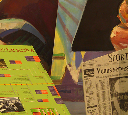
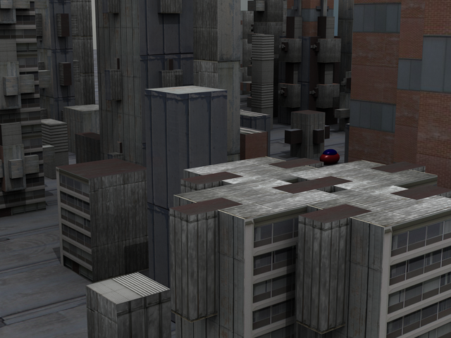
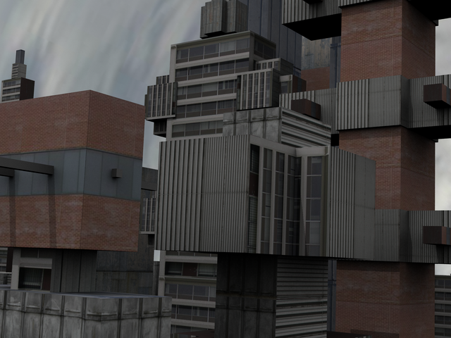
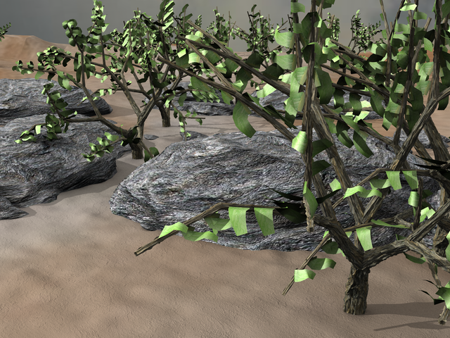
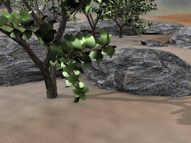
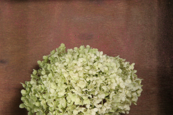
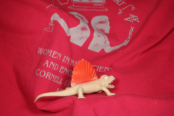
Figure 1: Image sequences from the Middlebury database. One frame of each sequence is displayed. Top and from left to right: Venus, Urban2, Urban3, Rubber Whale; Bottom and from left to right: Grove3, Grove2, Hydrangea, Dimetrodon.

The most common used measure of performance for optical flow is the angular error (AE) between a flow vector $(u_{1},u_{2})$ and the ground truth flow $(gt_{1},gt_{2})$. It is the angle in $3D$ between $(u_{1},u_{2},1)$ and $(gt_{1},gt_{2},1)$. The AE is calculated by the following formula:

$${\rm AE}={\arccos}\left(\frac{1+u_{1}\times gt_{1}+u_{2}\times gt_{2}}{\sqrt{1+u_{1}^{2}+u_{2}^{2}}\sqrt{1+gt_{1}^{2}+gt_{2}^{2}}}\right).$$ (41)

The popularity of this measure is due to the seminal work by Barron et al [3]. This measure provides a relative measure of performance that avoids the divide by zero problem for zero flows. Errors in large flows are penalized less in AE than errors in small flows. The AE also contains an arbitrary scaling constant $1$ to convert the units from pixels to degrees.

A complementar measure is usually used, which is, the End Point Error (EPE) defined by

$${\rm EPE}=\sqrt{(u_{1}-gt_{1})^{2}+(u_{2}-gt_{2})^{2}}.$$ (42)

This measure may be more appropriate for some applications. Therefore we report both herein.

These measures are computed at each pixel and consequently the corresponding averages of AE (AAE) and of EPE (AEPE) are used. In some cases the standard deviations of AE (SDAE) will be also presented.

In the next experiments some of the values of the parameters in our model are chosen to be the values for which the TV-L1 method performs better, according to [18], in order to compare its performance with the performance of the TV-L1-SB method. Regarding the choice of the parameters $\lambda_{\ell}$, $\ell=1,2$, associated with split Bregman method, we assume

$$\lambda_{SB}=\lambda_{1}=\lambda_{2}.$$

Note that the parameters $\lambda_{\ell}$, $\ell=1,2$ are related, respectively, with the flow velocity $u_{\ell},\ell=1,2$. In [11] the authors have found that for a faster convergence a good choice for the split Bregman parameter, $\lambda_{SB}$, can be $\lambda_{SB}={2}/{\theta}.$ For the TV-L1-SB method this seems to be also a suitable choice.

We start with some discussion about the choice of the split Bregman parameter $\lambda_{SB}$. Figure 2 displays the results of the experiments done for the Rubber-Whale sequence (see Figure 1). It shows the performance of the TV-L1-SB method for different values of $\lambda_{SB}$ when $\theta=0.4$ and for different data attachment weights $\lambda$. The tightness parameter $\theta=0.4$ is chosen according to [18] as mentioned previously. It can be seen that the TV-L1-SB method performs better for the set of split Bregman values, $1\leq\lambda_{SB}\leq 10$, reaching its best between $3$ and $10$.

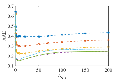
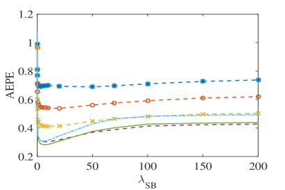
Figure 2: Performance of the TV-L1-SB method for the Rubber Whale sequence: $\theta=0.4$ and $Nwraps=Nscales=5$. The method performs better for values of the split Bregman parameter $3\leq\lambda_{SB}\leq 10$. Plots for different values of the data attachment weight $\lambda$: $\lambda=0.03(\--*)$; $\lambda=0.05(\--o)$; $\lambda=0.1(\--\times)$; $\lambda=0.3(\--\--)$; $\lambda=0.5(\--)$; $\lambda=1(\--\cdot\--)$.

In Table 2 we compare the TV-L1-SB method with the TV-L1 method for the image sequences presented in Figure 1. For each image sequence we have chosen the parameters $\lambda$ (data attachment weight) and $\theta$ (tightness) for which the TV-L1 method performs better. The split Bregman parameter $\lambda_{SB}$ needed in the TV-L1-SB method is assumed to be $10$ for all image sequences. The results point out the TV-L1-SB method performs better than the TV-L1 method.

Method AAE AEPE SDAE Data Method AAE AEPE SDAE Data Grove2 6 scales RubberWhale 4 scales TV-L1 0.7070 2.1876 0.4351 $\lambda=0.3$ TV-L1 0.2281 0.4155 0.2724 $\lambda=0.4$ TV-L1-SB 0.5443 1.7974 0.4283 $\theta=0.3$ TV-L1-SB 0.1530 0.2905 0.2406 $\theta=0.4$ Grove3 4 scales Hydrangea 4 scales TV-L1 0.5856 2.8451 0.4803 $\lambda=0.5$ TV-L1 0.4185 2.1619 0.2798 $\lambda=0.1$ TV-L1-SB 0.4198 2.4920 0.3984 $\theta=0.4$ TV-L1-SB 0.3107 1.9487 0.2049 $\theta=0.8$ Urban2 6 scales Dimetrodon 5 scales TV-L1 0.6623 7.4200 0.5477 $\lambda=0.5$ TV-L1 0.4282 1.1511 0.3109 $\lambda=0.3$ TV-L1-SB 0.5319 7.1988 0.4941 $\theta=0.3$ TV-L1-SB 0.3356 1.0051 0.2724 $\theta=0.3$ Urban3 5 scales Venus 4 scales TV-L1 0.9403 6.4110 0.6624 $\lambda=0.9$ TV-L1 0.6693 2.8136 0.4318 $\lambda=0.4$ TV-L1-SB 0.7890 5.9711 0.6606 $\theta=0.7$ TV-L1-SB 0.4629 2.4105 0.3757 $\theta=0.6$

Table 2: Errors AAE, AEPE and SDAE for the TV-L1 method and the TV-L1-SB method for the sequence of images presented in Figure 1.

To have a more complete perspective between the differences on the performance of both methods we exhibit in Figures 3 and 4 additional results, with different values of $\theta$ and $\lambda$ in the Rubber Whale case and for $\lambda_{SB}=10$. The results confirm the TV-L1-SB method presents smaller errors in general. By running these experiments we have observed that the TV-L1-SB method is slower if the split Bregman parameter $\lambda_{SB}$ is very far away from the estimate $2/\theta$. We have executed the algorithm for a fixed $\lambda_{SB}=10$ and as $\theta$ becomes larger the method becomes slower, suggesting the parameter $\lambda_{SB}$ should be adjusted depending on $\theta$, for a faster convergence. We did not adjust the parameter $\lambda_{SB}$ to plot Figures 3 and 4 to emphasize the effect of only changing the data attachment weight parameter $\lambda$ and tightness parameter $\theta$.

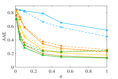
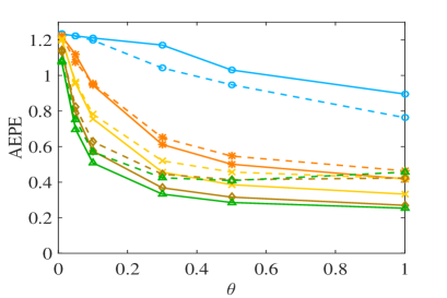
Figure 3: Errors AAE and AEPE for the Rubber Whale sequence. The tightness parameter $\theta$ changes and $Nwraps=5$, $Nscales=4$. The TV-L1 method is represented by the dashed lines $(\--\--)$ and the TV-L1-SB method by the solid lines $(\--)$. The different values of the data attachment weight $\lambda$ are marked by different symbols: $\lambda=0.01(o)$, $\lambda=0.05(*)$, $\lambda=0.1(\times)$, $\lambda=0.2(\diamond)$, $\lambda=0.3(\ \hat{}\ )$.

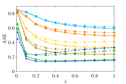
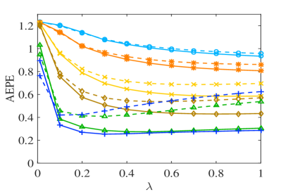
Figure 4: Errors AAE and AEPE for the Rubber Whale sequence: The data attachment weight parameter $\lambda$ changes and $Nwraps=5$, $Nscales=4$. The TV-L1 method is represented by the dashed lines $(\--\--)$ and the TV-L1-SB method by the solid lines $(\--)$. The different values of the tightness parameter $\theta$ are marked with different symbols: $\theta=0.01(o)$, $\theta=0.02(*)$, $\theta=0.05(\times)$, $\theta=0.1(\diamond)$, $\theta=0.5(\ \hat{}\ )$, $\theta=1(\ +\ )$.

4.2 The effect of the fractional regularization operator

The main purpose of this section is to present the effect of the parameter $\alpha$ in the estimation of the optical flow. Only partial regions of the image are used in order to show efficiently the influence of $\alpha$. Three main regions are considered: with edges, corners and flat that can also present high or low texture and motion discontinuities.

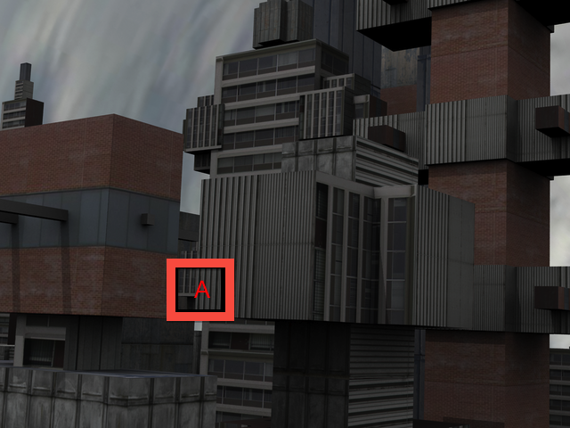
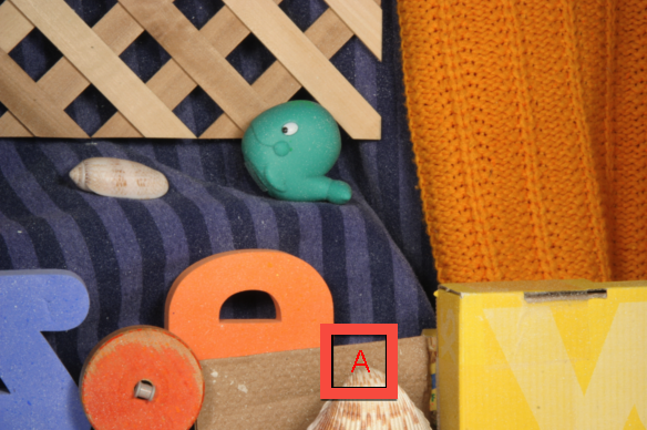
Figure 5: The regions considered for each image sequence are marked as regions A (red) or B (blue). From left to right: Grove2 (Regions A and B), Urban3 (Region A), Hydrangea (Regions A and B) and Rubber Whale (Region A).

We start to discuss the results for the image sequences considered the most difficult from the Middleburry database, which are Grove and Urban. For these data images the optical flow methods usually perform worst. As described in [2] Grove contains a close up view of a tree, with a substantial parallax and motion discontinuities and Urban contains the image of a city with substantial motion discontinuities, a large motion range and an independently moving object. We consider the image sequences Grove2 and Urban3 displayed in Figure 5.

For the sequence Grove2 we have selected two types of regions for discussion: one represents a flat region (marked as region B) and the other one represents a region with edges and a parallax effect (marked as region A). We assume $N_{wraps}=5$, $N_{scales}=5$ and the tightness parameter $\theta$ and the data attachment weight parameter $\lambda$ are chosen according to Table 2, that is, $\theta=0.3$ and $\lambda=0.3$. In Figures 6(a) and 6(b) we report the errors for the optical flow computed in the two regions of Grove2 for different values of $\alpha$. We have also done tests for different values of the split Bregman parameter, $\lambda_{SB}$, in particular with values between $1$ and $10$. In Figure 6(a), related to the region A marked in Figure 5, we only plot the results for the split Bregman parameter $\lambda_{SB}=5$, the value for which we have obtained the best results. It is shown the best result, represented by the smallest errors, have been reached at $\alpha=1.2$ for the error AAE and at $\alpha=1.4$ for the error AEPE. In general, the best results are for values of $\alpha$ between $1$ and $1.5$. In Figure 6(b), we show what happens for the flat region, region B of Grove2. The best results in this case have been obtained for $\lambda_{SB}=7$ and the errors AAE and AEPE are smaller for $\alpha=0$.

We turn now to the image sequence Urban3. In this image we have selected only a region, region A, with corners and edges. In Figure 6(c) we plot the results for this region, when $\lambda=0.9$ and $\theta=0.7$. The best $\lambda_{SB}$ value is in this case $1$. We remind the value of $\lambda_{SB}$ seems to be related to the value of $\theta$, that is, it should be close to $2/\theta$. The best results are attained for $\alpha$ between $1.5$ and $2$ and in particular for $\alpha=1.5$. The variations of the errors in terms of $\alpha$ are not smooth as in the case of the sequence Grove2 for the region A shown in Figure 6(a).

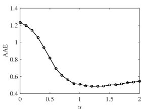
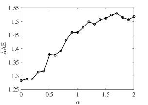
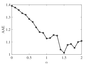
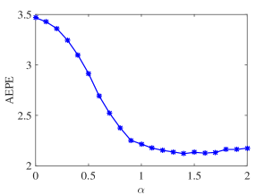
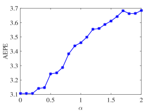
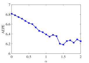
(a)                                                   (b)                                                   (c)

Figure 6: (a) Grove2 – Part A. For $\lambda=0.3$ and $\theta=0.3$. Best results for $\lambda_{SB}=5$. AAE: best result for $\alpha=1.2$. AEPE: best result for $\alpha=1.4$; (b) Grove2 – Part B. For $\lambda=0.3$ and $\theta=0.3$. Best results for $\lambda_{SB}=7$. AAE: best result for $\alpha=0$. AEPE: best result for $\alpha=0$; (c) Urban3 – Part A. For $\lambda=0.9$ and $\theta=0.7$. Best results for $\lambda_{SB}=1$. AAE: best result for $\alpha=1.5$. AEPE: best result for $\alpha=1.5$.

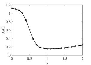
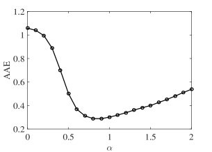
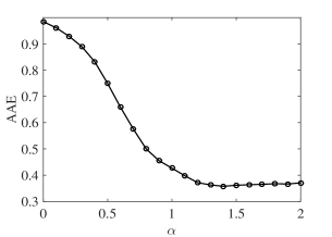
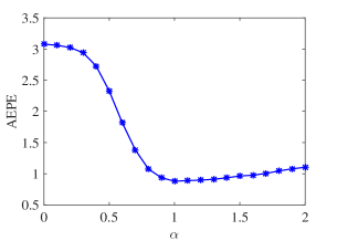
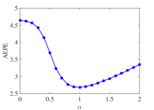
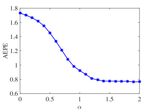
(a)                                                   (b)                                                   (c)

Figure 7: (a) Hydrangea – PartA. For $\lambda=0.1$ and $\theta=0.8$. Best results for $\lambda_{SB}=3$. AAE: best result for $\alpha=1$. AEPE: best result for $\alpha=1$; (b) Hydrangea – PartB. For $\lambda=0.1$ and $\theta=0.8$. Best results for $\lambda_{SB}=10$. AAE: best result for $\alpha=0.9$. AEPE: best result for $\alpha=1$; (c) Rubber Whale – PartA. For $\lambda=0.4$ and $\theta=0.4$. Best results for $\lambda_{SB}=2$. AAE: best result for $\alpha=1.4$. AEPE: best result for $\alpha=1.4$.

In Figure 7 we present the results for two other sequences: Hydrangea, Figures 7(a) and 7(b), and Rubber Whale, Figure 7(c). The regions analysed are marked in Figure 5. For Hydrangea, regions A and B, the errors are smaller for values of $\alpha$ around $1$ and for Rubber Whale, region A, the smaller errors are for $1.4$. In the Rubber Whale case although the best value is reached at $\alpha=1.4$ and not $\alpha=1$, we note that for these values of $\alpha$ the differences between the errors are less relevant than for the sequences Grove2 and Urban3.

We have seen that for flat regions the best $\alpha$ is close to $0$, see Figure 6(b), for edges is between $1$ and $1.5$, see Figures 6(a) and 7(c), and for corners between $1.5$ and $2$, see Figure 6(c). Additionally the results for the most difficult datasets, Grove2 and Urban3, highlights the advantage of using the fractional order $\alpha$, by presenting significantly smaller errors for values of $\alpha$ that are different from $1$.

5 Final Remarks

We have presented and tested a new algorithm to solve an optical flow model. The novelty of this work is twofold: there is the inclusion of a regularisation operator which uses fractional derivatives and the application of the split Bregman technique.

It is difficult to recover accurately motion fields and these difficulties arise from scene geometry and texture complexity. We have seen that the parameter $\alpha$, related to the order of the fractional regularisation operator, can be adjusted to deal with different regions. This motivates a future work, to further explore the potential of the proposed approach, that is to build a feature based algorithm. This algorithm would present a robust approach that integrates region tracking, that is, it would be able to detect a priori the type of structures the image presents and to adjust the parameter $\alpha$ accordingly. Additionally, faster iterative methods can be developed to solve the iterative system related to the fractional Euler-Lagrange equation.

References

• [1] O.P. Agrawal, Formulation of Euler-Lagrange equations for fractional variational problems, J. Math. Anal. Appl. 272 (2002) 368–379.
• [2] S. Baker, D. Scharstein, J.P. Lewis, S. Roth, M.J. Black, R. Szeliski, A database and evaluation methodology for optical flow, Int. J. Comput. Vis. 92 (2011) 1–31.
• [3] J. Barron, D. Fleet, S. Beauchemin, Performance of optical flow tecnhiques, Int. J. Comput. Vis. 12 (1994) 43–77.
• [4] M. Black, P. Anandan, The robust estimation of multiple motions: Parametric and piecewise-smooth flow fields, Comput. Vis. Image Und. 63 (1996) 75–104.
• [5] L.M. Bregman, The relaxation method of finding the common point of convex sets and its application to the solution of problems in convex programming, USSR Computational Mathematics and Mathematical Physics 7 (1967) 200-217.
• [6] L. Bourdin, J. Cresson, I. Greff, P. Inizan, Variational integrator for fractional Euler-Lagrange equations, Appl. Numer. Math. 71 (2015) 14–23.
• [7] A. Chambolle An algorithm for total variation minimization and applications. J. Math. Imaging Vis. 20 (2004) 89–97.
• [8] R.H. Chan, A. Lanza, S. Morigi, F. Sgallari, An adaptive strategy for the restoration of textured images using fractional order regularization, Numer. Math. Theor. Meth. Appl. 6 (2013) 276–296.
• [9] D. Chen, H. Sheng, YQ. Chen, D. Xue, Fractional-order variational optical flow model for motion estimation, Phil. Trans. R. Soc. A 371 (2013) 20120148.
• [10] W. Enkelman, Investigations of multigrid algorithms for the estimation of optical flow fields in image sequences. In Proceeding of the workshop on motion: representations and analysis (1986) 81–87.
• [11] T. Goldstein, S. Osher. The split Bregman method for L1-regularized problems, SIAM J. Imaging Sci. 2 (2009) 323 – 343.
• [12] B. K. P. Horn, B. G. Schunck. Determining optical flow, Artif. Intell. 17 (1981) 185–203.
• [13] A.A. Kilbas, H.M. Srivastava, J.J. Trujillo. Theory and applications of fractional differential equations, Elsevier, 2006.
• [14] E. Meinhardt-Llopis, J. Sánchez Pérez, D. Kondermann. Horn-Schunck optical flow with a multi-scale strategy. Image Processing On Line 3 (2013) 151–172.
• [15] I. Podlubny, Fractional Differential Equations, Academic Press, San Diego, 1999.
• [16] P. D. Romero, F. V. Candela, Blind deconvolution models regularized by fractional powers of the Laplacian, J. Math. Imaging Vis. 32 (2008)181-191.
• [17] S.G. Samko, A.A. Kilbas, O.I. Marichev, Fractional Integrals and derivatives: theory and applications, Gordon and Breach Science Publishers, 1993.
• [18] J. Sánchez, E. Meinhardt-Llopis, G. Facciolo, TV-L1 optical flow estimation, Image Processing On Line 3 (2013) 137–150.
• [19] E. Sousa, How to approximate the fractional derivative of order $1<\alpha\leq 2$, Int. J. Bifurcation Chaos 22 (2012) 1250075.
• [20] J. Weickert, A. Bruhn, T. Brox, N. Papenberg. A survey on variational optic flow methods for small displacements, In Mathematical Models for Registration and Applications to Medical Imaging Math. Ind. 10, O. Scherzer, ed., Springer, Berlin, Heidelberg (2006) 103–136.
• [21] C. Zach, T. Pock, and H. Bischof. A duality based approach for realtime TV-L1 optical flow. In Ann. Symp. German Association Patt. Recogn, (2007) 214–223.
• [22] J. Zhang, Z. Wei, L. Xiao, Adaptive fractional-order multi-scale method for image denoising, J. Math. Imaging Vis. 43 (2012) 39–49.