Sublabel–Accurate Relaxation of Nonconvex Energies

Abstract

We propose a novel spatially continuous framework for convex relaxations based on functional lifting. Our method can be interpreted as a sublabel–accurate solution to multilabel problems. We show that previously proposed functional lifting methods optimize an energy which is linear between two labels and hence require (often infinitely) many labels for a faithful approximation. In contrast, the proposed formulation is based on a piecewise convex approximation and therefore needs far fewer labels – see Fig. 1. In comparison to recent MRF-based approaches, our method is formulated in a spatially continuous setting and shows less grid bias. Moreover, in a local sense, our formulation is the tightest possible convex relaxation. It is easy to implement and allows an efficient primal-dual optimization on GPUs. We show the effectiveness of our approach on several computer vision problems.

1 Introduction

Energy minimization methods have become the central paradigm for solving practical problems in computer vision. The energy functional can often be written as the sum of a data fidelity and a regularization term. One of the most popular regularizers is the total variation (${TV}$) due to its many favorable properties [4]. Hence, an important class of optimization problems is given as

$$\underset{u:\Omega\rightarrow\Gamma}{\min}\leavevmode\nobreak\ \int_{\Omega}\rho(x,u(x))\leavevmode\nobreak\ \mathrm{d}x+\lambda\leavevmode\nobreak\ {TV}(u),$$ (1)

defined for functions $u$ with finite total variation, arbitrary, possibly nonconvex dataterms $\rho:\Omega\times\Gamma\rightarrow\mathbb{R}$, label spaces $\Gamma$ which are closed intervals in $\mathbb{R}$, $\Omega\subset\mathbb{R}^{d}$, and $\lambda\in\mathbb{R}^{+}$. The multilabel interpretation of the dataterm is that $\rho(x,u(x))$ represents the costs of assigning label $u(x)$ to point $x$. For (weakly) differentiable functions $TV(u)$ equals the integral over the norm of the derivative, and therefore favors a spatially coherent label configuration. The difficultly of minimizing the nonconvex energy (1) has motivated researchers to develop convex reformulations.

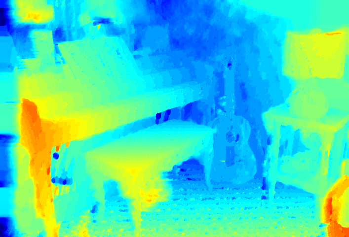
(a)

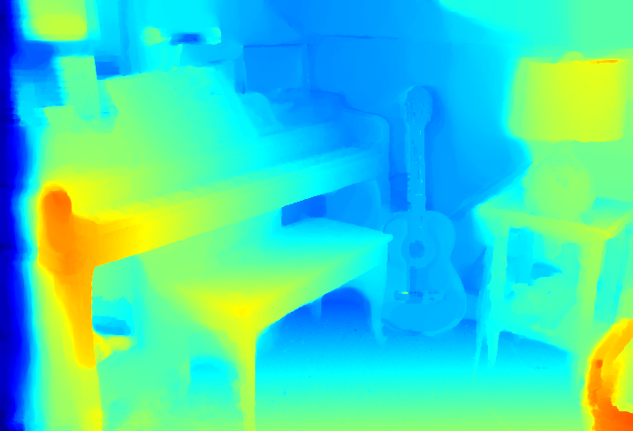
(b)

Figure 1: We propose a convex relaxation for the variational model (1), which opposed to existing functional lifting methods [17, 18] allows continuous label spaces even after discretization. Our method (here applied to stereo matching) avoids label space discretization artifacts, while saving on memory and runtime.

Convex representations of (1) and more general related energies have been studied in the context of the calibration method for the Mumford-Shah functional [1]. Based on these works, relaxations for the piecewise constant [15] and piecewise smooth Mumford-Shah functional [16] have been proposed. Inspired by Ishikawa’s graph-theoretic globally optimal solution to discrete variants of (1), continuous analogues have been considered by Pock et al. in [17, 18]. Continuous relaxations for multilabeling problems with finite label spaces $\Gamma$ have also been studied in [11].

Interestingly, the discretization of the aforementioned continuous relaxations is very similar to the linear programming relaxations proposed for MAP inference in the Markov Random Field (MRF) community [10, 22, 24, 26]. Both approaches ultimately discretize the range $\Gamma$ into a finite set of labels. A closer analysis of these relaxations reveals, however, that they are not well-suited to represent the continuous valued range that we face in most computer vision problems such as stereo matching or optical flow. More specifically, the above relaxations are not designed to assign meaningful cost values to non-integral configurations. As a result, a large number of labels is required to achieve a faithful approximation. Solving real-world vision problems therefore entails large optimization problems with high memory and runtime requirement. To address this problem, Zach and Kohli [27], Zach [25] and Fix and Agarwal [7] introduced MRF-based approaches which retain continuous label spaces after discretization. For manifold-valued labels, this issue was addressed by Lellmann et al. [12], however with the sole focus on the regularizer.

1.1 Contributions

We propose the first sublabel–accurate convex relaxation of nonconvex problems in a spatially continuous setting. It exhibits several favorable properties:

• In contrast to existing spatially continuous lifting approaches [17, 18], the proposed method provides substantially better solutions with far fewer labels – see Fig. 1. This provides savings in runtime and memory.

• In Sec. 3 we show that the functional lifting methods [17, 18] are a special case of the proposed framework.

• In Sec. 3 we show that, in a local sense, our formulation is the tightest convex relaxation which takes dataterm and regularizer into account separately. It is unknown whether this “local convex envelope” property also holds for the discrete approach [27].

• Our formulation is compact and requires only half the amount of variables for the dataterm than the formulation in [27]. We prove that the sublabel–accurate total variation can be represented in a very simple way, introducing no overhead compared to [17, 18]. In contrast, the regularizer in [27] is much more involved.

• Since our method is derived in a spatially continuous setting, the proposed approach easily allows different gradient discretizations. In contrast to [25, 27] the regularizer is isotropic leading to noticeably less grid bias.

2 Notation and Mathematical Preliminaries

We make heavy use of the convex conjugate, which is given as $f^{*}(y)=\sup_{x\in\mathbb{R}^{n}}\leavevmode\nobreak\ \langle y,x\rangle-f(x)$ for functions $f:\mathbb{R}^{n}\rightarrow\mathbb{R}\cup\{\infty\}$. The biconjugate $f^{**}$ denotes its convex envelope, i.e. the largest lower-semicontinuous convex under-approximation of $f$. For a set $C$ we denote by $\delta_{C}$ the function which maps any element from $C$ to $0$ and is $\infty$ otherwise. For a comprehensive introduction to convex analysis, we refer the reader to [19]. Vector valued functions $\boldsymbol{u}:\Omega\to\mathbb{R}^{k}$ are written in bold symbols. If it is clear from the context, we will drop the $x\in\Omega$ inside the functions, e.g., we write $\rho(u)$ for $\rho(x,u(x))$.

3 Functional Lifting

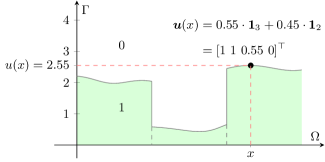
Figure 2: Lifted representation. Instead of optimizing over the function $u:\Omega\rightarrow\Gamma$, we optimize over all possible graph functions $\boldsymbol{u}:\Omega\rightarrow\mathbb{R}^{k}$ (in this example $k=4$). The central idea behind our approach is the finite dimensional representation of $\boldsymbol{u}$ at every point $x\in\Omega$.

(a)

(b)

Figure 3: We show the nonconvex energy $\rho(u)$ at a fixed point $x\in\Omega$ (red dashed line in both plots) from the stereo matching experiment in Fig. 9 over the full range of $270$ disparities. The black dots indicate the positions of the labels and the black curves show the approximations used by the respective methods. Fig. 3a: The baseline lifting method [17] uses a piecewise linear approximation with labels as nodes. Fig. 3b: The proposed method uses an optimal piecewise convex approximation. As we can see, the piecewise convex approximation is closer to the original nonconvex energy and therefore more accurate.

To derive a convex representation of (1), we rely on the framework of functional lifting. The idea is to reformulate the optimization problem in a higher dimensional space, in which the convex envelope approximates the nonconvex energy better than the one of the original low dimensional energy. We start by sampling the range $\Gamma$ at $L=k+1$ labels $\gamma_{1}<\ldots<\gamma_{L}\in\Gamma$. This partitions the range into $k$ intervals $\Gamma_{i}=[\gamma_{i},\gamma_{i+1}]$ so that $\Gamma=\Gamma_{1}\cup\ldots\cup\Gamma_{k}$. Clearly, any value in the range of $u:\Omega\to\Gamma$ can be written as

$$u(x)=\gamma_{i}^{\alpha}:=\gamma_{i}+\alpha(\gamma_{i+1}-\gamma_{i}),$$ (2)

for $\alpha\in[0,1]$ and some label index $1\leq i\leq k$. We represent such a value in the range $\Gamma$ by a $k$-dimensional vector

$$\boldsymbol{u}(x)=\mathbf{1}_{i}^{\alpha}:=\alpha\mathbf{1}_{i}+(1-\alpha)\mathbf{1}_{i-1},$$ (3)

where $\mathbf{1}_{i}$ denotes a vector starting with $i$ ones followed by $k-i$ zeros. We call $\boldsymbol{u}:\Omega\to\mathbb{R}^{k}$ the lifted representation of $u$, representing the graph of $u$. This notation is depicted in Fig. 2 for $k=4$. Back-projecting the lifted $\boldsymbol{u}(x)$ to the range of $u$ using the layer cake formula yields a one-to-one correspondence between $u(x)=\gamma_{i}^{\alpha}$ and $\boldsymbol{u}(x)=\mathbf{1}_{i}^{\alpha}$ via

$$u(x)=\gamma_{1}+\sum_{i=1}^{k}{\boldsymbol{u}}_{i}(x)(\gamma_{i+1}-\gamma_{i}).$$ (4)

We now formulate problem (1) in terms of such graph functions, a technique that is common in the theory of Cartesian currents [8].

3.1 Convexification of the Dataterm

For now, we consider a fixed $x\in\Omega$. Then the dataterm from (1) is a possibly nonconvex real-valued function (cf. Fig. 3) that we seek to minimize over a compact interval $\Gamma$:

$$\underset{u\in\Gamma}{\min}\leavevmode\nobreak\ \rho(u).$$ (5)

Due to the one-to-one correspondence between $\gamma_{i}^{\alpha}$ and $\mathbf{1}_{i}^{\alpha}$ it is clear that solving problem (5) is equivalent to finding a minimizer of the lifted energy:

$$\boldsymbol{\rho}(\boldsymbol{u})=\underset{1\leq i\leq k}{\min}\leavevmode\nobreak\ \boldsymbol{\rho}_{i}(\boldsymbol{u}),$$ (6)

$$\boldsymbol{\rho}_{i}(\boldsymbol{u})=\begin{cases}\rho(\gamma_{i}^{\alpha}),\qquad&\text{if }\leavevmode\nobreak\ \boldsymbol{u}=\mathbf{1}_{i}^{\alpha},\leavevmode\nobreak\ \alpha\in[0,1],\\ \infty,&\text{else.}\end{cases}$$ (7)

Note that the constraint in (7) is essentially the nonconvex special ordered set of type 2 (SOS2) constraint [3]. More precisely, we demand that the derivative $\partial_{\gamma}\boldsymbol{u}$ is zero, except for two neighboring elements, which add up to one. In the following proposition, we derive the tightest convex relaxation of $\boldsymbol{\rho}$.

Proposition 1.

The convex envelope of (6) is given as:

$$\boldsymbol{\rho}^{**}(\boldsymbol{u})=\underset{\boldsymbol{v}\in\mathbb{R}^{k}}{\sup}\leavevmode\nobreak\ \langle\boldsymbol{u},\boldsymbol{v}\rangle-\underset{1\leq i\leq k}{\max}\leavevmode\nobreak\ \boldsymbol{\rho}_{i}^{*}(\boldsymbol{v}),$$ (8)

where the conjugate of the individual $\boldsymbol{\rho}_{i}$ is

$$\boldsymbol{\rho}_{i}^{*}(\boldsymbol{v})=c_{i}(\boldsymbol{v})+\rho_{i}^{*}\left(\frac{\boldsymbol{v}_{i}}{\gamma_{i+1}-\gamma_{i}}\right),$$ (9)

with $c_{i}(\boldsymbol{v})=\langle\mathbf{1}_{i-1},\boldsymbol{v}\rangle-\frac{\gamma_{i}}{\gamma_{i+1}-\gamma_{i}}$ and $\rho_{i}=\rho+\delta_{\Gamma_{i}}$.

Proof.

See appendix. ∎

The above proposition reveals that the convex relaxation implicitly convexifies the dataterm $\rho$ on each interval $\Gamma_{i}$. The equality $\rho_{i}^{*}=\rho_{i}^{***}$ implies that starting with $\rho_{i}$ yields exactly the same convex relaxation as starting with $\rho_{i}^{**}$.

Corollary 1.

If $\rho$ is linear on each $\Gamma_{i}$, then the convex envelopes of $\boldsymbol{\rho}(\boldsymbol{u})$ and $\boldsymbol{\sigma}(\boldsymbol{u})$ coincide, where the latter is:

$$\boldsymbol{\sigma}(\boldsymbol{u})=\begin{cases}\rho(\gamma_{i}^{\alpha}),\qquad&\text{if }\leavevmode\nobreak\ \exists i:\;\boldsymbol{u}=\mathbf{1}_{i}^{\alpha},\leavevmode\nobreak\ \alpha\in\{0,1\},\\ \infty,&\text{else.}\end{cases}$$ (10)

Proof.

Consider an additional constraint $\delta_{\{\gamma_{i},\gamma_{i+1}\}}$ for each $\rho_{i}$, which corresponds to selecting $\alpha\in\{0,1\}$ in (7). The fact that our relaxation is independent of whether we choose $\rho_{i}$ or $\rho_{i}^{**}$, along with the fact that the convex hull of two points is a line, yields the assertion. ∎

For the piecewise linear case, it is possible to find an explicit form of the biconjugate.

Proposition 2.

Let us denote by $\textbf{r}\in\mathbb{R}^{k}$ the vector with

$$\textbf{r}_{i}=\rho(\gamma_{i+1})-\rho(\gamma_{i}),\ \ 1\leq i\leq k.$$ (11)

Under the assumptions of Prop. 1, one obtains:

$$\boldsymbol{\sigma}^{**}(\boldsymbol{u})=\begin{cases}\rho(\gamma_{1})+\langle\boldsymbol{u},\textbf{r}\rangle,\qquad&\text{if }\leavevmode\nobreak\ \boldsymbol{u}_{i}\geq\boldsymbol{u}_{i+1},\boldsymbol{u}_{i}\in[0,1],\\ \infty,&\text{else.}\end{cases}$$ (12)

Proof.

See appendix. ∎

Up to an offset (which is irrelevant for the optimization), one can see that (12) coincides with the dataterm of [15], the discretizations of [17, 18], and – after a change of variable – with [11]. This not only proves that the latter is optimizing a convex envelope, but also shows that our method naturally generalizes the work from piecewise linear to arbitrary piecewise convex energies. Fig. 3a and Fig. 3b illustrate the difference of $\boldsymbol{\sigma}^{**}$ and $\boldsymbol{\rho}^{**}$ on the example of a nonconvex stereo matching cost.

Because our method allows arbitrary convex functions on each $\Gamma_{i}$, we can prove that, for the two label case, our approach optimizes the convex envelope of the dataterm.

Proposition 3.

In the case of binary labeling, i.e., $L=2$, the convex envelope of (6) reduces to

$$\boldsymbol{\rho}^{**}(\boldsymbol{u})=\rho^{**}\left(\gamma_{1}+\boldsymbol{u}(\gamma_{2}-\gamma_{1})\right),\text{ with }\boldsymbol{u}\in[0,1].$$ (13)

Proof.

See appendix. ∎

3.2 A Lifted Representation of the Total Variation

We now want to find a lifted convex formulation that emulates the total variation regularization in (1). We follow [5] and define an appropriate integrand of the functional

$$TV(\boldsymbol{u})=\int_{\Omega}\boldsymbol{\Phi}(x,D\boldsymbol{u}),$$ (14)

where the distributional derivative $D\boldsymbol{u}$ is a finite $\mathbb{R}^{k\times d}$-valued Radon measure [2]. We define

$$\boldsymbol{\Phi}(\boldsymbol{g})=\underset{1\leq i\leq j\leq k}{\min}\leavevmode\nobreak\ \boldsymbol{\Phi}_{i,j}(\boldsymbol{g}).$$ (15)

The individual $\boldsymbol{\Phi}_{i,j}:\mathbb{R}^{k\times d}\to\mathbb{R}\cup\{\infty\}$ are given by:

$$\boldsymbol{\Phi}_{i,j}(\boldsymbol{g})=\begin{cases}\left|\gamma_{i}^{\alpha}-\gamma_{j}^{\beta}\right|\cdot|\nu|_{2},\qquad&\text{ if }\boldsymbol{g}=(\mathbf{1}_{i}^{\alpha}-\mathbf{1}_{j}^{\beta})\leavevmode\nobreak\ \nu^{\mathsf{T}},\\ \infty,&\text{ else,}\end{cases}$$ (16)

for some $\alpha,\beta\in[0,1]$ and $\nu\in\mathbb{R}^{d}$. The intuition is that $\Phi_{i,j}$ penalizes a jump from $\gamma_{i}^{\alpha}$ to $\gamma_{j}^{\beta}$ in the direction of $\nu$. Since $\boldsymbol{\Phi}$ is nonconvex we compute the convex envelope.

Proposition 4.

The convex envelope of (15) is

$$\boldsymbol{\Phi}^{**}(\boldsymbol{g})=\underset{\boldsymbol{q}\in\mathcal{K}}{\sup}\leavevmode\nobreak\ \langle\boldsymbol{q},\boldsymbol{g}\rangle,$$ (17)

where $\mathcal{K}\subset\mathbb{R}^{k\times d}$ is given as:

$$\mathcal{K}=\left\{\boldsymbol{q}\in\vphantom{\left|\boldsymbol{q}^{\mathsf{T}}(\mathbf{1}_{i}^{\alpha}-\mathbf{1}_{j}^{\beta})\right|_{2}}\right. \mathbb{R}^{k\times d}\leavevmode\nobreak\ \Big{|}\leavevmode\nobreak\$$ (18)

$$\left|\boldsymbol{q}^{\mathsf{T}}(\mathbf{1}_{i}^{\alpha}-\mathbf{1}_{j}^{\beta})\right|_{2}\leq\left|\gamma_{i}^{\alpha}-\gamma_{j}^{\beta}\right|,$$

$$\left.\vphantom{\left|\boldsymbol{q}^{\mathsf{T}}(\mathbf{1}_{i}^{\alpha}-\mathbf{1}_{j}^{\beta})\right|_{2}}\forall\leavevmode\nobreak\ 1\leq i\leq j\leq k,\leavevmode\nobreak\ \forall\alpha,\beta\in[0,1]\right\}.$$

Proof.

See appendix. ∎

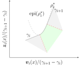
(a)

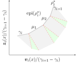
(b)

Figure 4: Illustration of the epigraph projection. In the left subfigure the projection onto the epigraph of the conjugate of a convex quadratic $\rho_{i}$ is shown. In the right subfigure the piecewise linear case is illustrated. In the both cases all points that lie in the gray sets are orthogonally projected onto the respective linear parts whereas the points that lie in the green sets are projected onto the parabolic part (in the quadratic case) respectively the kinks (in the piecewise linear case). In the piecewise linear case the green sets are normal cones. The red dashed lines correspond to the boundary cases. $\gamma_{i}$, $\gamma_{i+1}$, $\mu_{1}$, $\mu_{2}$ are the slopes of the segments of $\rho_{i}^{*}$ respectively the (sub-)label positions of $\rho_{i}$.

The set $\mathcal{K}$ from Eq. (36) involves infinitely many constraints which makes numerical optimization difficult. As the following proposition reveals, the infinite number of constraints can be reduced to only linearly many, allowing to enforce the constraint $\boldsymbol{q}\in\mathcal{K}$ exactly.

Proposition 5.

In case the labels are ordered, i.e., $\gamma_{1}<\gamma_{2}<\ldots<\gamma_{L}$, then the constraint set $\mathcal{K}$ from Eq. (36) is equal to

$$\mathcal{K}=\{\boldsymbol{q}\in \mathbb{R}^{k\times d}\leavevmode\nobreak\ \mid\leavevmode\nobreak\ |\boldsymbol{q}_{i}|_{2}\leq\gamma_{i+1}-\gamma_{i},\leavevmode\nobreak\ \forall i\}.$$ (19)

Proof.

See appendix. ∎

This shows that the proposed regularizer coincides with the total variation from [5], where it has been derived based on (16) for $\alpha$ and $\beta$ restricted to $\{0,1\}$. Prop. 19 together with Prop. 13 show that for $k=1$ our formulation amounts to unlifted ${TV}$ optimization with a convexified dataterm.

4 Numerical Optimization

(a)

(b)

(c)

(d)

(e)

(f)

Figure 5: Denoising comparison. We compare the proposed method to the baseline method [17] on the convex ROF problem. We show the time in seconds required for each method to produce a solution within a certain energy gap to the optimal solution. As the baseline method optimizes a piecewise linear approximation of the quadratic dataterm, it fails to reach that optimality gap even for $L=256$ (indicated by $t=\infty$). In contrast, while the proposed lifting method can solve a large class of non-convex problems, it is almost as efficient as direct methods on convex problems.

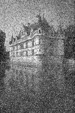
(a)

(b)

(c)

(d)

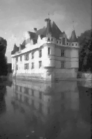
(e)

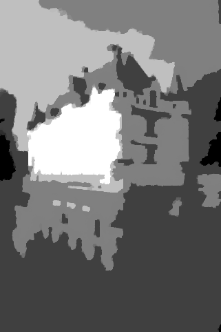
(f)

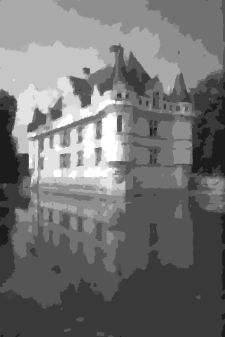
(g)

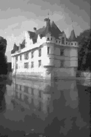
(h)

Figure 6: Denoising using a robust truncated quadratic dataterm. The top row shows the input image along with the result obtained by our approach for a varying number of labels $L$. The bottom row illustrates the results obtained by the baseline method [17]. The energy of the final solution as well as the total runtime are given below each image.

Discretizing $\Omega\subset\mathbb{R}^{d}$ as a $d$-dimensional Cartesian grid, the relaxed energy minimization problem becomes

$$\min_{\boldsymbol{u}:\Omega\to\mathbb{R}^{k}}\sum_{x\in\Omega}\boldsymbol{\rho}^{**}(x,\boldsymbol{u}(x))+\boldsymbol{\Phi}^{**}(x,\nabla\boldsymbol{u}(x)),$$ (20)

where $\nabla$ denotes a forward-difference operator with $\nabla\boldsymbol{u}:\Omega\to\mathbb{R}^{k\times d}$. We rewrite the dataterm given in equation (8) by replacing the pointwise maximum over the conjugates $\boldsymbol{\rho}_{i}^{*}$ with a maximum over a real number $q\in\mathbb{R}$ and obtain the following saddle point formulation of problem (20):

$$\min_{\boldsymbol{u}:\Omega\to\mathbb{R}^{k}}\max_{\begin{subarray}{c}(\boldsymbol{v},q)\in\mathcal{C}\\[1.42262pt] \boldsymbol{p}:\Omega\to\mathcal{K}\end{subarray}}\langle\boldsymbol{u},\boldsymbol{v}\rangle-\sum_{x\in\Omega}q(x)+\langle\boldsymbol{p},\nabla\boldsymbol{u}\rangle,$$ (21)

$$\mathcal{C}=\{ (\boldsymbol{v},q):\Omega\to\mathbb{R}^{k}\times\mathbb{R}\mid q(x)\geq\boldsymbol{\rho}_{i}^{*}(\boldsymbol{v}(x)),\ \forall x,\forall i\}.$$ (22)

We numerically compute a minimizer of problem (21) using a first-order primal-dual method [6, 16] with diagonal preconditioning [14] and adaptive steps [9]. It basically alternates between a gradient descent step in the primal variable and a gradient ascent step in the dual variable. Subsequently the dual variables are orthogonally projected onto the sets $\mathcal{C}$ respectively $\mathcal{K}$. The projection onto the set $\mathcal{K}$ is a simple $\ell_{2}$-ball projection. To simplify the projection onto $\mathcal{C}$, we transform the $k$-dimensional epigraph constraints in (22) into $1$-dimensional scaled epigraph constraints by introducing an additional variable $z:\Omega\to\mathbb{R}^{k}$ with:

$$\boldsymbol{z}_{i}(x)=\left[q(x)-c_{i}\left(\boldsymbol{v}(x)\right)\right]\left(\gamma_{i+1}-\gamma_{i}\right).$$ (23)

Using equation (9) we can now rewrite the constraints in (22) as

$$\frac{\boldsymbol{z}_{i}(x)}{\gamma_{i+1}-\gamma_{i}}\geq\rho_{i}^{*}\left(\frac{\boldsymbol{v}_{i}(x)}{\gamma_{i+1}-\gamma_{i}}\right).$$ (24)

We implement the newly introduced equality constraints (23) introducing a Lagrange multiplier $\boldsymbol{s}:\Omega\to\mathbb{R}^{k}$. It remains to discuss the orthogonal projections onto the epigraphs of the conjugates $\rho_{i}^{*}$. Currently we support quadratic and piecewise linear convex pieces $\rho_{i}$. For the piecewise linear case, the conjugate $\rho_{i}^{*}$ is a piecewise linear function with domain $\mathbb{R}$. The slopes correspond to the $x$-positions of the sublabels and the intercepts correspond to the function values at the sublabel positions.

The conjugates as well as the epigraph projections of both, a quadratic and a piecewise linear piece are depicted in Fig. 4. For the quadratic case, the projection onto the epigraph of a parabola is computed using [23, Appendix B.2].

(a)

(b)

(c)

(d)

(e)

(f)

(g)

(h)

(i)

(j)

(k)

(l)

Figure 7: Comparison to the MRF approach presented in [27]. The first row shows DC-Linear, second row DC-MRF and third row our results for $4$, $8$, $16$ and $32$ convex pieces on the truncated quadratic energy (26). Below the figures we show the final nonconvex energy. We achieve competitive results while using a more compact representation and generalizing to isotropic regularizers.

5 Experiments

We implemented the primal-dual algorithm in CUDA to run on GPUs. For $d=2$, our implementation of the functional lifting framework [17], which will serve as a baseline method, requires $4N(L-1)$ optimization variables, while the proposed method requires $6N(L-1)+N$ variables, where $N$ is the number of points used to discretize the domain $\Omega\subset\mathbb{R}^{d}$. As we will show, our method requires much fewer labels to yield comparable results, thus, leading to an improvement in accuracy, memory usage, and speed.

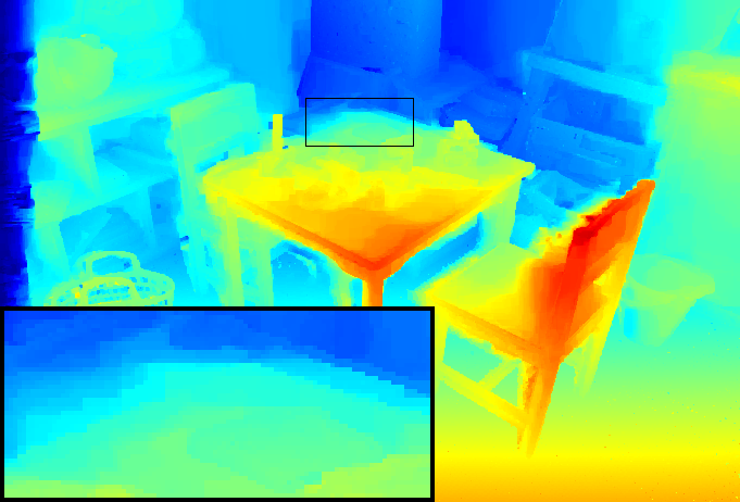
(a)

(b)

Figure 8: We compare the proposed relaxation with anistropic regularizer to isotropic regularization on the stereo matching example. Using an anisotropic formulation as in [27] leads to grid bias.

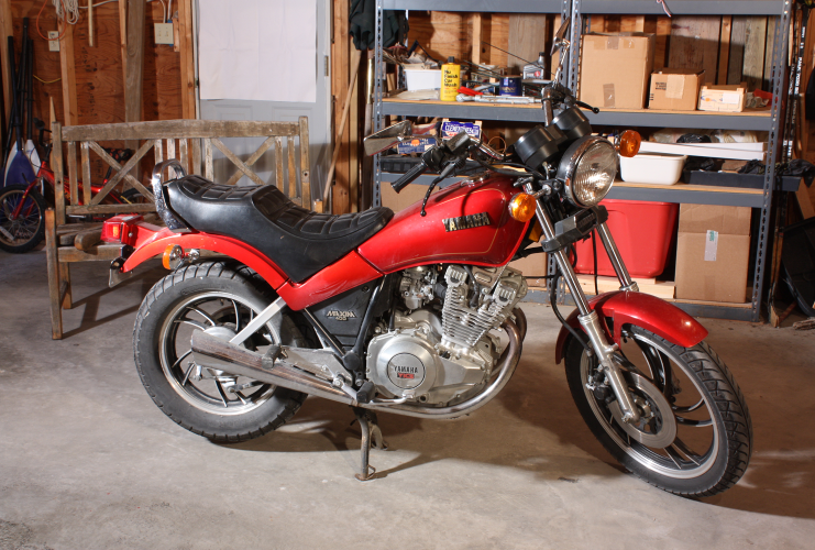
(a) One of the input images

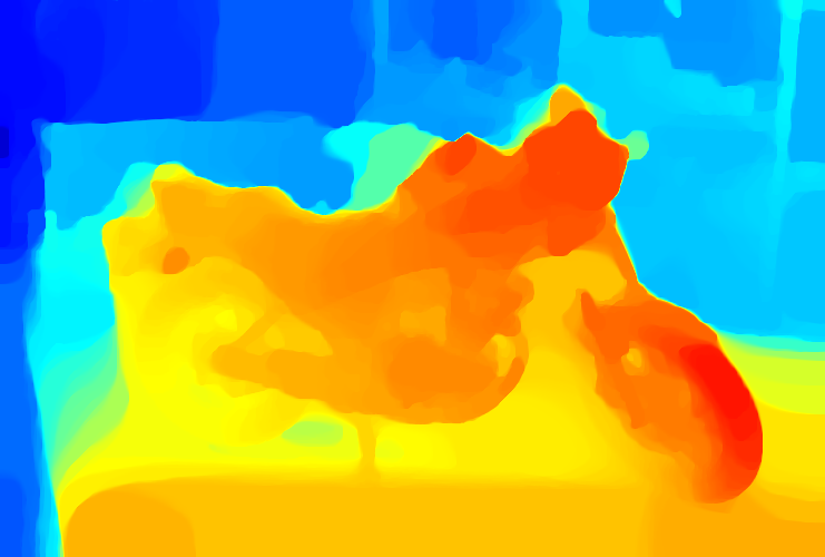
(b) Proposed ($L=2$)

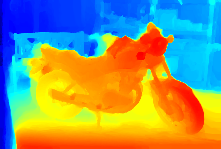
(c) Proposed ($L=4$)

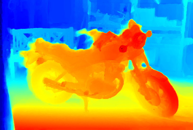
(d) Proposed ($L=8$)

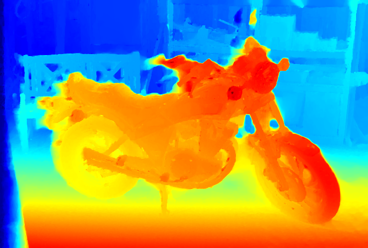
(e) Proposed ($L=16$)

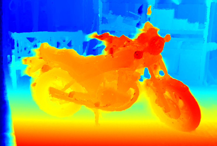
(f) Proposed ($L=32$)

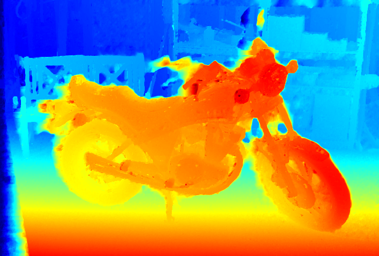
(g) Baseline ($L=270$)

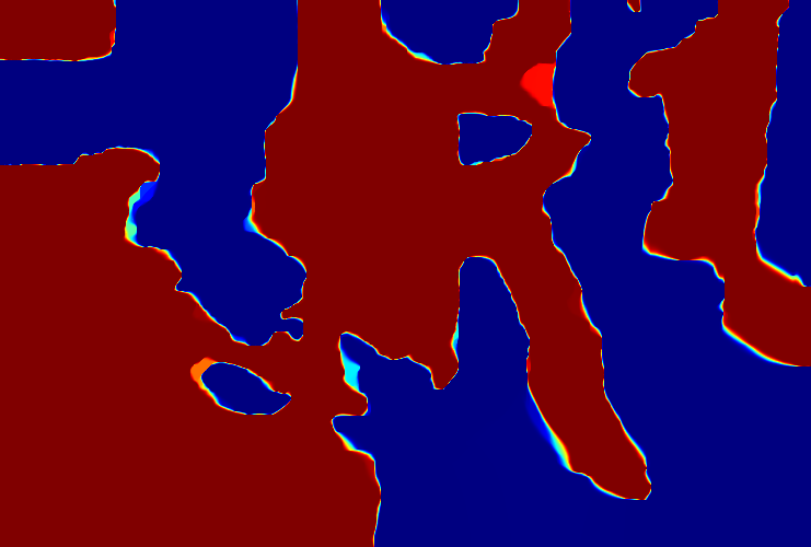
(h) Baseline ($L=2$)

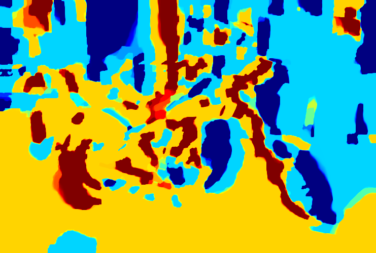
(i) Baseline ($L=4$)

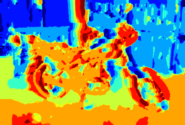
(j) Baseline ($L=8$)

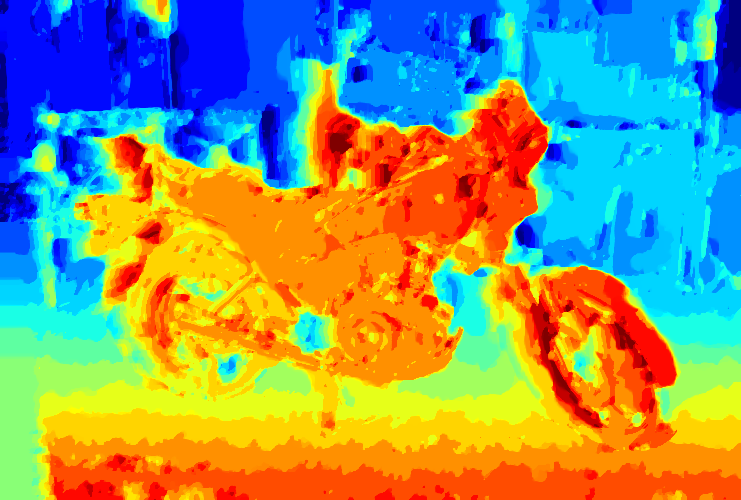
(k) Baseline ($L=16$)

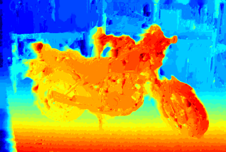
(l) Baseline ($L=32$)

Figure 9: Stereo comparison. We compare the proposed method to the baseline method on the example of stereo matching. The first column shows one of the two input images and below the baseline method with the full number of labels. The proposed relaxation requires much fewer labels to reach a smooth depth map. Even for $L=32$, the label space discretization of the baseline method is strongly visible, while the proposed method yields a smooth result already for $L=8$.

5.1 Rudin-Osher-Fatemi Model

As a proof of concept, we first evaluate the novel relaxation on the well-known Rudin-Osher-Fatemi (ROF) model [20]. It corresponds to (1) with the following dataterm:

$$\rho(x,u(x))=\left(u(x)-f(x)\right)^{2},$$ (25)

where $f:\Omega\rightarrow\mathbb{R}$ denotes the input data. While there is no practical use in applying convex relaxation methods to an already convex problem such as the ROF model, the purpose of this is two-fold. Firstly, it allows us to measure the overhead introduced by our method by comparing it to standard convex optimization methods which do not rely on functional lifting. Secondly, we can experimentally verify that the relaxation is tight for a convex dataterm.

In Fig. 5 we solve (25) directly using the primal-dual algorithm [9], using the baseline functional lifting method [17] and using our proposed algorithm. First, the globally optimal energy was computed using the direct method with a very high number of iterations. Then we measure how long each method took to reach this global optimum to a fixed tolerance.

The baseline method fails to reach the global optimum even for $256$ labels. While the lifting framework introduces a certain overhead, the proposed method finds the same globally optimal energy as the direct unlifted optimization approach and generalizes to nonconvex energies.

5.2 Robust Truncated Quadratic Dataterm

The quadratic dataterm in (25) is often not well suited for real-world data as it comes from a pure Gaussian noise assumption and does not model outliers. We now consider a robust truncated quadratic dataterm:

$$\rho(x,u(x))=\frac{\alpha}{2}\min\left\{(u(x)-f(x))^{2},\nu\right\}.$$ (26)

To implement (26), we use a piecewise polynomial approximation of the dataterm. In Fig. 6 we degraded the input image with additive Gaussian and salt and pepper noise. The parameters in (26) were chosen as $\alpha=25$, $\nu=0.025$ and $\lambda=1$. The proposed method requires significantly less labels to find lower energies than the baseline method.

5.3 Comparison to the Method of Zach and Kohli

We remark that Prop. 18 and Prop. 19 hold for arbitrary convex one-homogeneous functionals $\phi(\nu)$ instead of $|\nu|_{2}$ in equation (16). In particular, they hold for the anisotropic total variation $\phi(\nu)=|\nu|_{1}$. This generalization allows us to directly compare our convex relaxation to the MRF approach of Zach and Kohli [27]. In Fig. 7 we show the results of optimizing the two models entitled “DC-Linear” and “DC-MRF” proposed in [27], and of our proposed method with anisotropic regularization on the robust truncated denoising energy (26). We picked the parameters as $\alpha=0.2$, $\nu=500$, and $\lambda=1$. The label space is also chosen as $\Gamma=[0,256]$ as described in [27].

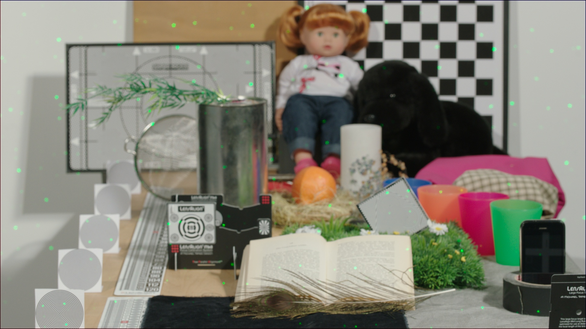
(a) One of the input images

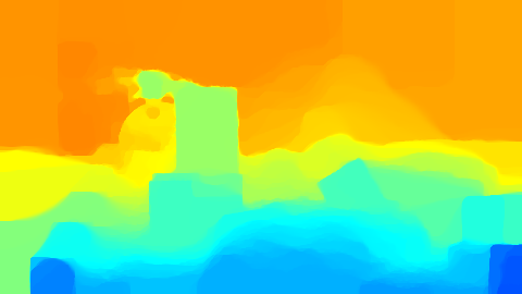
(b) Proposed ($L=2$)

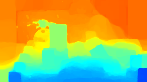
(c) Proposed ($L=4$)

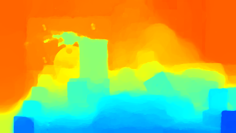
(d) Proposed ($L=8$)

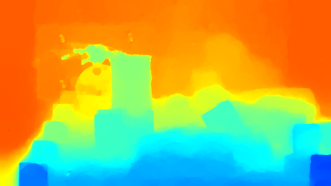
(e) Proposed ($L=16$)

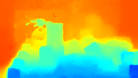
(f) Proposed ($L=32$)

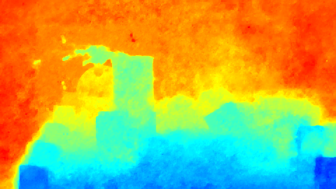
(g) Baseline ($L=374$)

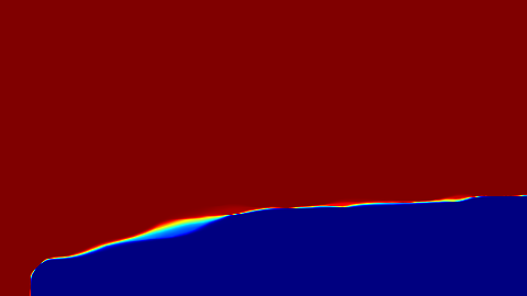
(h) Baseline ($L=2$)

(i) Baseline ($L=4$)

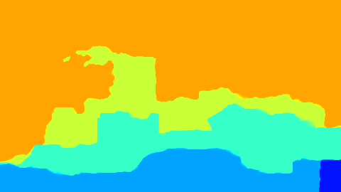
(j) Baseline ($L=8$)

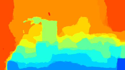
(k) Baseline ($L=16$)

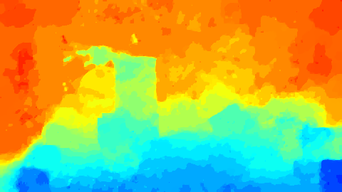
(l) Baseline ($L=32$)

Figure 10: Depth from focus comparison. We compare our method to the baseline approach on the problem of depth from focus. First column: one of the 374 differently focused input images and the baseline method for full number of labels. Following columns: proposed relaxation (top row) vs. baseline (bottom row) for 2, 4, 8, 16 and 32 labels each.

Overall, all the energies are better than the ones reported in [27]. It can be seen from Fig. 7 that the proposed relaxation is competitive to the one proposed in [27]. In addition, The proposed relaxation uses a more compact representation and extends to isotropic regularizers. To illustrate the advantages of isotropic regularizations, Fig. 8a and Fig. 8b show a comparison of our proposed method for isotropic and anisotropic regularization in the next section.

5.4 Stereo Matching

Given a pair of rectified images, the task of finding a correspondence between the two images can be formulated as an optimization problem over a scalar field $u:\Omega\rightarrow\Gamma$ where each point $u(x)\in\Gamma$ denotes the displacement along the epipolar line associated with each $x\in\Omega$. The overall cost functional fits Eq. (1). In our experiments, we computed $\rho(x,u(x))$ for $270$ disparities on the Middlebury stereo benchmark [21] in a $4\times 4$ patch using a truncated sum of absolute gradient differences. For the dataterm of the proposed relaxation, we convexify the matching cost $\rho$ in each range $\Gamma_{i}$ by numerically computing the convex envelope using the gift wrapping algorithm.

The first row in Fig. 9 shows the result of the proposed relaxation using the convexified energy between two labels. The second row shows the baseline approach using the same amount of labels. Even for $L=2$, the proposed method produces a reasonable depth map while the baseline approach basically corresponds to a two region segmentation.

5.5 Phase Unwrapping

Many sensors such as time-of-flight cameras or interferometric synthetic aperture radar (SAR) yield cyclic data lying on the circle ${{\mathcal{S}}^{1}}$. Here we consider the task of total variation regularized unwrapping. As is shown on the left in Fig. 11, the dataterm is a nonconvex function where each minimum corresponds to a phase shift by $2\pi$:

$$\rho\left(x,u(x)\right)=d_{{{\mathcal{S}}^{1}}}\left(u(x),f(x)\right)^{2}.$$ (27)

For the experiments, we approximated the nonconvex energy by quadratic pieces as depicted in Fig. 11. The label space is chosen as $\Gamma=[0,4\pi]$ and the regularization parameter was set to $\lambda=0.005$. Again, it is visible in Fig. 11 that the baseline method shows label space discretization and fails to unwrap the depth map correctly if the number of labels is chosen too low. The proposed method yields a smooth unwrapped result using only $8$ labels.

5.6 Depth From Focus

In depth from focus the task is to recover the depth of a scene, given a stack of images each taken from a constant position but in a different focal setting, so that in each image only the objects of a certain depth are sharp. We achieve this by estimating the depth of a point by locally maximizing its contrast over the set of images. We compute the cost by using the modified Laplacian function [13] as a contrast measure. Similar to the stereo experiments, we convexify the cost on each label range by computing the convex hull. The results are shown in Fig. 10. While the baseline method clearly shows the label space discretization, the proposed approach yields a smooth depth map. Since the proposed method uses a convex lower bound of the lifted energy, the regularizer has slightly more influence on the final result. This explains why the resulting depth maps in Fig. 10 and Fig. 9 look overall less noisy.

6 Conclusion

(a) Piecewise convex energy

(b) Input image

(c) Ground truth

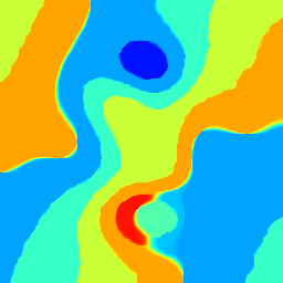
(d) Baseline ($L=8$)

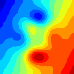
(e) Baseline ($L=16$)

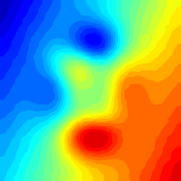
(f) Baseline ($L=32$)

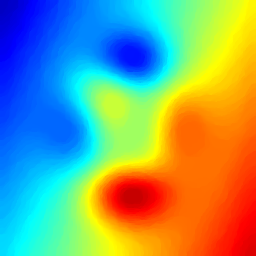
(g) Proposed ($L=8$)

Figure 11: We show the piecewise convex approximation of the phase unwrapping energy, followed by the cyclic input image and the unwrapped ground truth. With only 8 labels, the proposed method already yields a smooth reconstruction. The baseline method fails to unwrap the heightmap correctly using $8$ labels, and for $16$ and $32$ labels, the discretization is still noticable.

In this work we proposed a tight convex relaxation that can be interpreted as a sublabel–accurate formulation of classical multilabel problems. We showed that the local convex envelope involves infinitely many constraints, however we proved that it suffices to consider linearly many of those. The final formulation is a simple saddle-point problem that admits fast primal-dual optimization. Our method maintains sublabel accuracy even after discretization and for that reason outperforms existing spatially continuous methods. Interesting directions for future work include higher dimensional label spaces, manifold valued data and more general regularizers.

Appendix A Appendix

Proof of Proposition 1.

The proof follows from a direct calculation. We start with the definition of the biconjugate:

$$\boldsymbol{\rho}^{**}(\boldsymbol{u}) =\underset{\boldsymbol{v}\in\mathbb{R}^{k}}{\sup}\leavevmode\nobreak\ \langle\boldsymbol{u},\boldsymbol{v}\rangle-\left(\underset{1\leq i\leq k}{\min}\leavevmode\nobreak\ \boldsymbol{\rho}_{i}(\boldsymbol{u})\right)^{*}$$ (28)

$$=\underset{\boldsymbol{v}\in\mathbb{R}^{k}}{\sup}\leavevmode\nobreak\ \langle\boldsymbol{u},\boldsymbol{v}\rangle-\underset{1\leq i\leq k}{\max}\leavevmode\nobreak\ \boldsymbol{\rho}_{i}^{*}(\boldsymbol{u}).$$

This shows the first equation inside the proposition. For the individual $\boldsymbol{\rho}_{i}^{*}$ we again start with the definition of the convex conjugate:

$$\boldsymbol{\rho}_{i}^{*}(\boldsymbol{v}) =\underset{\alpha\in[0,1]}{\sup}\leavevmode\nobreak\ \langle\alpha\mathbf{1}_{i}+(1-\alpha)\mathbf{1}_{i-1},\boldsymbol{v}\rangle-$$ (29)

$$\qquad\qquad\qquad\rho(\alpha\gamma_{i+1}+(1-\alpha)\gamma_{i})$$

$$=\underset{\alpha\in[0,1]}{\sup}\leavevmode\nobreak\ \langle\mathbf{1}_{i-1},\boldsymbol{v}\rangle+\alpha\boldsymbol{v}_{i}-\rho(\gamma_{i}^{\alpha}).$$

Applying the substitution $\gamma_{i}^{\alpha}=\alpha\gamma_{i+1}+(1-\alpha)\gamma_{i}$ and consequently $\alpha=\frac{\gamma_{i}^{\alpha}-\gamma_{i}}{\gamma_{i+1}-\gamma_{i}}$ yields:

$$\boldsymbol{\rho}_{i}^{*}(\boldsymbol{v})=\underset{\gamma_{i}^{\alpha}\in\Gamma_{i}}{\sup}\leavevmode\nobreak\ \langle\mathbf{1}_{i-1},\boldsymbol{v}\rangle+\frac{\gamma_{i}^{\alpha}-\gamma_{i}}{\gamma_{i+1}-\gamma_{i}}\boldsymbol{v}_{i}-\rho(\gamma_{i}^{\alpha})$$ (30)

$$= \langle\mathbf{1}_{i-1},\boldsymbol{v}\rangle-\frac{\gamma_{i}}{\gamma_{i+1}-\gamma_{i}}\boldsymbol{v}_{i}+\underset{\gamma_{i}^{\alpha}\in\Gamma_{i}}{\sup}\leavevmode\nobreak\ \gamma_{i}^{\alpha}\frac{\boldsymbol{v}_{i}}{\gamma_{i+1}-\gamma_{i}}-\rho(\gamma_{i}^{\alpha})$$

$$= \langle\mathbf{1}_{i-1},\boldsymbol{v}\rangle-\frac{\gamma_{i}}{\gamma_{i+1}-\gamma_{i}}\boldsymbol{v}_{i}+(\rho+\delta_{\Gamma_{i}})^{*}\left(\frac{\boldsymbol{v}_{i}}{\gamma_{i+1}-\gamma_{i}}\right)$$

$$= :c_{i}(\boldsymbol{v})+\rho_{i}^{*}\left(\frac{\boldsymbol{v}_{i}}{\gamma_{i+1}-\gamma_{i}}\right).$$

∎

Proof of Proposition 2.

It is easy to see that

$$\boldsymbol{\sigma}^{*}(\boldsymbol{v})=\max_{i\in\{1,...,L\}}\left(\sum_{l=1}^{i-1}\boldsymbol{v}_{l}-\rho(\gamma_{i})\right).$$

To compute the biconjugate, we write any input argument $\boldsymbol{u}=\sum_{i=1}^{k}\mu_{i}\mathbf{1}_{i+1}$, and use $\boldsymbol{\sigma}^{**}=\boldsymbol{\rho}^{**}$ to obtain

$$\boldsymbol{\rho}^{**}(\boldsymbol{u}) =\sup_{\boldsymbol{v}}\langle\boldsymbol{u},\boldsymbol{v}\rangle-\max_{i\in\{1,...,L\}}\left(\sum_{l=1}^{i-1}\boldsymbol{v}_{l}-\rho(\gamma_{i})\right)$$

$$=\sup_{\boldsymbol{v}}\sum_{i=1}^{k}\mu_{i}\sum_{l=1}^{i}\boldsymbol{v}_{l}-\max_{i\in\{1,...,L\}}\left(\sum_{l=1}^{i-1}\boldsymbol{v}_{l}-\rho(\gamma_{i})\right).$$

Instead of taking the supremum of all $\boldsymbol{v}$, we might as well take the supremum over all vectors p with $\textbf{p}_{i}=\sum_{l=1}^{i}\boldsymbol{v}_{l}$. Care has to be taken of the first summand in the second term of the above formulation. We obtain

$$\sup_{\boldsymbol{v}}\sum_{i=1}^{k}\mu_{i}\sum_{l=1}^{i}\boldsymbol{v}_{l}-\max_{i\in\{1,...,L\}}\left(\sum_{l=1}^{i-1}\boldsymbol{v}_{l}-\rho(\gamma_{i})\right),$$

$$= \sup_{\textbf{p}}\sum_{i=1}^{k}\mu_{i}\textbf{p}_{i}-\max_{i\in\{2,...,L\}}\max(\textbf{p}_{i-1}-\rho(\gamma_{i}),-\rho(\gamma_{1})),$$

$$= \sup_{\textbf{p}}\sum_{i=1}^{k}\mu_{i}\textbf{p}_{i}-\max_{i\in\{1,...,k\}}\max(\textbf{p}_{i}-\rho(\gamma_{i+1}),-\rho(\gamma_{1})),$$

$$= \sum_{i=1}^{k}\mu_{i}\;\rho(\gamma_{i+1})$$

$$+\sup_{\textbf{p}}\sum_{i=1}^{k}\mu_{i}\textbf{p}_{i}-\max_{i\in\{1,...,k\}}\max(\textbf{p}_{i},-\rho(\gamma_{1})),$$

Note that for any $\mu_{i}$ being negative, the supremum immediately yields infinity by taking $\textbf{p}_{i}\rightarrow-\infty$. Similarly, if $\sum_{i=1}^{k}\mu_{i}>1$ yields infinity by taking all $\textbf{p}_{i}\rightarrow\infty$. For $\mu_{i}\geq 0$ for all $i$, and $\sum_{i=1}^{k}\mu_{i}\leq 1$, we know that $\sum_{i=1}^{k}\mu_{i}\textbf{p}_{i}\leq(\max_{i}\textbf{p}_{i})\sum_{i=1}^{k}\mu_{i}$. Since equality can be obtained by choosing $\textbf{p}_{l}=\max_{i}\textbf{p}_{i}$ for all $l$, we can reduce the above supremum to

$$\sup_{z}\left(z\sum_{i=1}^{k}\mu_{i}-\max(z,-\rho(\gamma_{1}))\right)=\left(1-\sum_{i=1}^{k}\mu_{i}\right)\rho(\gamma_{1}),$$

where we used that the supremum over $z$ is attained at $z=-\rho(\gamma_{1})$ (still assuming that $\sum_{i=1}^{k}\mu_{i}\leq 1$). Let us now undo our change of variable. It is easy to see that $\mu_{k}=\boldsymbol{u}_{k}$, and $\mu_{i}=\boldsymbol{u}_{i}-\boldsymbol{u}_{i+1}$ for $i=1,...,k-1$. The latter leads to

$$\sum_{i=1}^{k}\mu_{i}\;\rho(\gamma_{i+1})+\left(1-\sum_{i=1}^{k}\mu_{i}\right)\rho(\gamma_{1})$$

$$=\rho(\gamma_{k+1})\boldsymbol{u}_{k}+\sum_{i=1}^{k-1}(\boldsymbol{u}_{i}-\boldsymbol{u}_{i+1})\;\rho(\gamma_{i+1})+(1-\boldsymbol{u}_{1})\rho(\gamma_{1})$$

$$=\rho(\gamma_{1})+\langle\boldsymbol{u},\textbf{r}\rangle,$$

for $\textbf{r}_{i}=\rho(\gamma_{i+1})-\rho(\gamma_{i})$. Considering the aforementioned constraints of $\mu_{i}\geq 0$, and $\sum_{i=1}^{k}\mu_{i}\leq 1$, we finally find

$$\boldsymbol{\rho}^{**}(\boldsymbol{u})=\begin{cases}\rho(\gamma_{1})+\langle\boldsymbol{u},\textbf{r}\rangle&\text{if }\leavevmode\nobreak\ 1\geq\boldsymbol{u}_{1}\geq...\geq\boldsymbol{u}_{k}\geq 0,\\ \infty,&\text{else.}\end{cases}$$

∎

Proof of Proposition 3.

For the special case $k=1$ the biconjugate from (28) is just:

$$\boldsymbol{\rho}^{**}(\boldsymbol{u})=\underset{\boldsymbol{v}\in\mathbb{R}}{\sup}\leavevmode\nobreak\ \boldsymbol{u}\boldsymbol{v}-\boldsymbol{\rho}_{1}^{*}(\boldsymbol{v})=\boldsymbol{\rho}_{1}^{**}(\boldsymbol{u}).$$ (31)

Now using the first line in (30), $\boldsymbol{\rho}_{1}^{**}$ becomes:

$$\boldsymbol{\rho}_{1}^{**}(\boldsymbol{u}) =\underset{\boldsymbol{v}\in\mathbb{R}}{\sup}\leavevmode\nobreak\ \boldsymbol{u}\boldsymbol{v}-\underset{\gamma\in\Gamma}{\sup}\leavevmode\nobreak\ \frac{\gamma-\gamma_{1}}{\gamma_{2}-\gamma_{1}}\boldsymbol{v}-\rho(\gamma)$$ (32)

$$=\underset{\boldsymbol{v}\in\mathbb{R}}{\sup}\leavevmode\nobreak\ \boldsymbol{v}\left(\boldsymbol{u}+\frac{\gamma_{1}}{\gamma_{2}-\gamma_{1}}\right)-\underset{\gamma\in\Gamma}{\sup}\leavevmode\nobreak\ \gamma\frac{\boldsymbol{v}}{\gamma_{2}-\gamma_{1}}-\rho(\gamma)$$

$$=\underset{\boldsymbol{v}\in\mathbb{R}}{\sup}\leavevmode\nobreak\ \boldsymbol{v}\left(\boldsymbol{u}+\frac{\gamma_{1}}{\gamma_{2}-\gamma_{1}}\right)-\rho^{*}\left(\frac{\boldsymbol{v}}{\gamma_{2}-\gamma_{1}}\right)$$

$$=\underset{\tilde{\boldsymbol{v}}\in\mathbb{R}}{\sup}\leavevmode\nobreak\ \tilde{\boldsymbol{v}}(\gamma_{1}+\boldsymbol{u}(\gamma_{2}-\gamma_{1}))-\rho^{*}(\tilde{\boldsymbol{v}})$$

$$=\rho^{**}(\gamma_{1}+\boldsymbol{u}(\gamma_{2}-\gamma_{1})),$$

where we used $\text{dom}(\rho)=\Gamma$ as well as the substitution $\boldsymbol{v}=(\gamma_{2}-\gamma_{1})\tilde{\boldsymbol{v}}$. ∎

Proof of Proposition 4.

We compute the individual conjugate as:

$$\boldsymbol{\Phi}_{i,j}^{*}(\boldsymbol{q})=\underset{\boldsymbol{g}\in\mathbb{R}^{d\times k}}{\sup}\langle g,\boldsymbol{q}\rangle-\boldsymbol{\Phi}_{i,j}(\boldsymbol{q})$$ (33)

$$=\underset{\alpha,\beta\in[0,1]}{\sup}\leavevmode\nobreak\ \underset{\nu\in\mathbb{R}^{d}}{\sup}\leavevmode\nobreak\ \langle\boldsymbol{q},(\mathbf{1}_{i}^{\alpha}-\mathbf{1}_{j}^{\beta})\nu^{\mathsf{T}}\rangle-\left|\gamma_{i}^{\alpha}-\gamma_{j}^{\beta}\right||\nu|_{2}$$

$$=\underset{\alpha,\beta\in[0,1]}{\sup}\leavevmode\nobreak\ \underset{\nu\in\mathbb{R}^{d}}{\sup}\leavevmode\nobreak\ \langle\boldsymbol{q}^{\mathsf{T}}(\mathbf{1}_{i}^{\alpha}-\mathbf{1}_{j}^{\beta}),\nu\rangle-\left|\gamma_{i}^{\alpha}-\gamma_{j}^{\beta}\right||\nu|_{2}$$

$$=\underset{\alpha,\beta\in[0,1]}{\sup}\leavevmode\nobreak\ \underset{\nu\in\mathbb{R}^{d}}{\sup}\leavevmode\nobreak\ \langle\boldsymbol{q}^{\mathsf{T}}(\mathbf{1}_{i}^{\alpha}-\mathbf{1}_{j}^{\beta}),\nu\rangle-\left|\gamma_{i}^{\alpha}-\gamma_{j}^{\beta}\right||\nu|_{2}.$$

The inner maximum over $\nu$ is the conjugate of the $\ell_{2}$-norm scaled by $\left|\gamma_{i}^{\alpha}-\gamma_{j}^{\beta}\right|$ evaluated at $\boldsymbol{q}^{\mathsf{T}}\left(\mathbf{1}_{i}^{\alpha}-\mathbf{1}_{j}^{\beta}\right)$. This yields:

$$\boldsymbol{\Phi}_{i,j}^{*}(\boldsymbol{q})=\begin{cases}0,&\text{if }\leavevmode\nobreak\ \left|\boldsymbol{q}^{\mathsf{T}}\left(\mathbf{1}_{i}^{\alpha}-\mathbf{1}_{j}^{\beta}\right)\right|_{2}\leq\left|\gamma_{i}^{\alpha}-\gamma_{j}^{\beta}\right|,\\ \leavevmode\nobreak\ &\hskip 99.58464pt\forall\alpha,\beta\in[0,1],\\ \infty,&\text{else.}\end{cases}$$ (34)

For the overall biconjugate we have:

$$\boldsymbol{\Phi}^{**}(\boldsymbol{g}) =\underset{\boldsymbol{q}\in\mathbb{R}^{k\times d}}{\sup}\leavevmode\nobreak\ \langle\boldsymbol{q},\boldsymbol{g}\rangle-\underset{1\leq i,j\leq k}{\max}\leavevmode\nobreak\ \boldsymbol{\Phi}_{i,j}^{*}(\boldsymbol{q})$$ (35)

$$=\underset{\boldsymbol{q}\in\mathcal{K}}{\sup}\leavevmode\nobreak\ \langle\boldsymbol{q},\boldsymbol{g}\rangle.$$

Since we have the $\max$ over all $1\leq i,j\leq k$ conjugates, the set $\mathcal{K}$ is given as the intersection of the sets described by the individual indicator functions $\boldsymbol{\Phi}_{i,j}$:

$$\mathcal{K}=\left\{\boldsymbol{q}\in\vphantom{\left|\boldsymbol{q}^{\mathsf{T}}(\mathbf{1}_{i}^{\alpha}-\mathbf{1}_{j}^{\beta})\right|_{2}}\right. \mathbb{R}^{k\times d}\leavevmode\nobreak\ \mid\leavevmode\nobreak\$$ (36)

$$\left|\boldsymbol{q}^{\mathsf{T}}(\mathbf{1}_{i}^{\alpha}-\mathbf{1}_{j}^{\beta})\right|_{2}\leq\left|\gamma_{i}^{\alpha}-\gamma_{j}^{\beta}\right|,$$

$$\left.\vphantom{\left|\boldsymbol{q}^{\mathsf{T}}(\mathbf{1}_{i}^{\alpha}-\mathbf{1}_{j}^{\beta})\right|_{2}}\forall\leavevmode\nobreak\ 1\leq i\leq j\leq k,\leavevmode\nobreak\ \forall\alpha,\beta\in[0,1]\right\}.$$

∎

Proof of Proposition 5.

First we rewrite (36) by expanding the matrix-vector product into sums:

$$\left|\sum_{l=j}^{i-1}\boldsymbol{q}_{l}+\alpha\boldsymbol{q}_{i}-\beta\boldsymbol{q}_{j}\right|_{2}\leq\left|\gamma_{i}^{\alpha}-\gamma_{j}^{\beta}\right|,$$ (37)

$$\forall\leavevmode\nobreak\ 1\leq j\leq i\leq k,\leavevmode\nobreak\ \forall\alpha,\beta\in[0,1].$$

Since the other cases for $1\leq i\leq j\leq k$ in (36) are equivalent to (37), it is enough to consider (37) instead of (36).

Let $\gamma_{1}<\gamma_{2}<\ldots<\gamma_{L}$. We show the equivalences:

(37)

$\Leftrightarrow$

$$\left|\sum_{l=j}^{i}\boldsymbol{q}_{l}\right|_{2}\leq\gamma_{i+1}-\gamma_{j},\leavevmode\nobreak\ \forall\leavevmode\nobreak\ 1\leq j\leq i\leq k.$$ (38)

$\Leftrightarrow$

$$|\boldsymbol{q}_{i}|_{2}\leq\gamma_{i+1}-\gamma_{i},\leavevmode\nobreak\ \forall\leavevmode\nobreak\ 1\leq i\leq k.$$ (39)

The direction “(37) $\Rightarrow$ (38)” follows by setting $\alpha=1$ and $\beta=0$ in (37), and “(38) $\Rightarrow$ (39)” follows by setting $i=j$ in (38).

The direction “(39) $\Rightarrow$ (38)” can be proven by a quick calculation:

$$\left|\sum_{l=j}^{i}\boldsymbol{q}_{l}\right|_{2}\leq\sum_{l=j}^{i}|\boldsymbol{q}_{l}|_{2}\leq\sum_{l=j}^{i}\gamma_{l+1}-\gamma_{l}=\gamma_{i+1}-\gamma_{j}.$$ (40)

It remains to show “(38) $\Rightarrow$ (37)”. We start with the case $j=i$:

$$|\alpha\boldsymbol{q}_{i}-\beta\boldsymbol{q}_{i}|_{2} =|\alpha-\beta||\boldsymbol{q}_{i}|_{2}$$ (41)

$$\leq|\alpha-\beta|(\gamma_{i+1}-\gamma_{i})$$

$$=|(\gamma_{i+1}-\gamma_{i})\alpha-(\gamma_{i+1}-\gamma_{i})\beta|$$

$$=|(\alpha-\beta)(\gamma_{i+1}-\gamma_{i})|=|\gamma_{i}^{\alpha}-\gamma_{i}^{\beta}|.$$

Now let $j<i$. Since $\gamma_{j}<\gamma_{i}$ it also holds that $\gamma_{j}^{\beta}\leq\gamma_{i}^{\alpha}$, thus it is equivalent to show (37) without the absolute value on the right hand side.

First we show that “(38) $\Rightarrow$ (37)” for $\beta\in\{0,1\}$ and $\alpha\in[0,1]$:

$$\left|\sum_{l=j+1}^{i-1}\boldsymbol{q}_{l}+\alpha\boldsymbol{q}_{i}+(1-\beta)\boldsymbol{q}_{j}\right|_{2}$$ (42)

$$\leq\left|\sum_{l=j+1}^{i-1}\boldsymbol{q}_{l}+(1-\beta)\boldsymbol{q}_{j}\right|_{2}+\alpha|\boldsymbol{q}_{i}|_{2}$$

$$\overset{\text{for }\beta=0\text{ or }\beta=1}{\leq}\gamma_{i}-\gamma_{j}^{\beta}+\alpha(\gamma_{i+1}-\gamma_{i})$$

$$=\gamma_{i}^{\alpha}-\gamma_{j}^{\beta}.$$

Using a similar argument we show that, using the above, “(38) $\Rightarrow$ (37)” for all $\alpha,\beta\in[0,1]$.

$$\left|\sum_{l=j+1}^{i-1}\boldsymbol{q}_{l}+\alpha\boldsymbol{q}_{i}+(1-\beta)\boldsymbol{q}_{j}\right|_{2}$$ (43)

$$\leq\left|\sum_{l=j+1}^{i-1}\boldsymbol{q}_{l}+\alpha\boldsymbol{q}_{i}\right|_{2}+(1-\beta)|\boldsymbol{q}_{j}|_{2}$$

$$\overset{\text{using }\eqref{eq:temp},\beta=1}{\leq}\gamma_{i}^{\alpha}-\gamma_{j+1}+(1-\beta)(\gamma_{j+1}-\gamma_{j})$$

$$=\gamma_{i}^{\alpha}-\gamma_{j}^{\beta}.$$

∎

References

- [1] G. Alberti, G. Bouchitté, and G. D. Maso. The calibration method for the Mumford-Shah functional and free-discontinuity problems. Calc. Var. Partial Dif., 3(16):299–333, 2003.
- [2] L. Ambrosio, N. Fusco, and D. Pallara. Functions of Bounded Variation and Free Discontinuity Problems. Oxford University Press, 2000.
- [3] E. Beale and J. Tomlin. Special facilities in a general mathematical programming system for nonconvex problems using ordered sets of variables. Proceedings of the fifth international conference on operational research, pages 447–454, 1970.
- [4] A. Chambolle, V. Caselles, D. Cremers, M. Novaga, and T. Pock. An introduction to total variation for image analysis. Theoretical foundations and numerical methods for sparse recovery, 9:263–340, 2010.
- [5] A. Chambolle, D. Cremers, and T. Pock. A convex approach to minimal partitions. SIAM Journal on Imaging Sciences, 5(4):1113–1158, 2012.
- [6] E. Esser, X. Zhang, and T. Chan. A general framework for a class of first order primal-dual algorithms for convex optimization in imaging science. SIAM Journal on Imaging Sciences, 3(4):1015–1046, 2010.
- [7] A. Fix and S. Agarwal. Duality and the continuous graphical model. In Computer Vision – ECCV 2014, volume 8691 of Lecture Notes in Computer Science, pages 266–281. Springer International Publishing, 2014.
- [8] M. Giaquinta, G. Modica, and J. Souček. Cartesian currents in the calculus of variations I, II., volume 37-38 of Ergebnisse der Mathematik und ihrer Grenzgebiete. 3. Springer-Verlag, Berlin, 1998.
- [9] T. Goldstein, E. Esser, and R. Baraniuk. Adaptive Primal-Dual Hybrid Gradient Methods for Saddle-Point Problems. arXiv Preprint, 2013.
- [10] H. Ishikawa. Exact optimization for Markov random fields with convex priors. IEEE Trans. Pattern Analysis and Machine Intelligence, 25(10):1333–1336, 2003.
- [11] J. Lellmann and C. Schnörr. Continuous multiclass labeling approaches and algorithms. SIAM J. Imaging Sciences, 4(4):1049–1096, 2011.
- [12] J. Lellmann, E. Strekalovskiy, S. Koetter, and D. Cremers. Total variation regularization for functions with values in a manifold. In ICCV, December 2013.
- [13] S. K. Nayar and Y. Nakagawa. Shape from focus. IEEE Trans. Pattern Anal. Mach. Intell., 16(8):824–831, Aug. 1994.
- [14] T. Pock and A. Chambolle. Diagonal preconditioning for first order primal-dual algorithms in convex optimization. In ICCV, pages 1762–1769, 2011.
- [15] T. Pock, A. Chambolle, H. Bischof, and D. Cremers. A convex relaxation approach for computing minimal partitions. In CVPR, pages 810–817, 2009.
- [16] T. Pock, D. Cremers, H. Bischof, and A. Chambolle. An algorithm for minimizing the piecewise smooth Mumford-Shah functional. In ICCV, 2009.
- [17] T. Pock, D. Cremers, H. Bischof, and A. Chambolle. Global solutions of variational models with convex regularization. SIAM J. Imaging Sci., 3(4):1122–1145, 2010.
- [18] T. Pock, T. Schoenemann, G. Graber, H. Bischof, and D. Cremers. A convex formulation of continuous multi-label problems. In European Conference on Computer Vision (ECCV), Marseille, France, October 2008.
- [19] R. T. Rockafellar. Convex Analysis. Princeton University Press, 1996.
- [20] L. I. Rudin, S. Osher, and E. Fatemi. Nonlinear total variation based noise removal algorithms. Physica D: Nonlinear Phenomena, 60(1):259–268, 1992.
- [21] D. Scharstein, H. Hirschmüller, Y. Kitajima, G. Krathwohl, N. Nešić, X. Wang, and P. Westling. High-resolution stereo datasets with subpixel-accurate ground truth. In German Conference on Pattern Recognition, volume 8753, pages 31–42. Springer, 2014.
- [22] M. Schlesinger. Sintaksicheskiy analiz dvumernykh zritelnikh signalov v usloviyakh pomekh (Syntactic analysis of two-dimensional visual signals in noisy conditions). Kibernetika, 4:113–130, 1976.
- [23] E. Strekalovskiy, A. Chambolle, and D. Cremers. Convex relaxation of vectorial problems with coupled regularization. SIAM Journal on Imaging Sciences, 7(1):294–336, 2014.
- [24] T. Werner. A linear programming approach to max-sum problem: A review. IEEE Trans. Pattern Anal. Mach. Intell., 29(7):1165–1179, July 2007.
- [25] C. Zach. Dual decomposition for joint discrete-continuous optimization. In AISTATS, pages 632–640, 2013.
- [26] C. Zach, C. Hane, and M. Pollefeys. What is optimized in tight convex relaxations for multi-label problems? In CVPR, pages 1664–1671, 2012.
- [27] C. Zach and P. Kohli. A convex discrete-continuous approach for markov random fields. In ECCV, volume 7577, pages 386–399. Springer Berlin Heidelberg, 2012.