Primordial non-Gaussianities of gravitational waves beyond Horndeski

Abstract

We clarify the features of primordial non-Gaussianities of tensor perturbations in Gao’s unifying framework of scalar-tensor theories. The general Lagrangian is given in terms of the ADM variables so that the framework maintains spatial covariance and includes the Horndeski theory and Gleyzes-Langlois-Piazza-Vernizzi (GLPV) generalization as specific cases. It is shown that the GLPV generalization does not give rise to any new terms in the cubic action compared to the case of the Horndeski theory, but four new terms appear in more general theories beyond GLPV. We compute the tensor 3-point correlation functions analytically by treating the modification to the dispersion relation as a perturbation. The relative change in the 3-point functions due to the modified dispersion relation is only mildly configuration-dependent. When the effect of the modified dispersion relation is small, there is only a single cubic term generating squeezed non-Gaussianity, which is the only term present in general relativity. The corresponding non-Gaussian amplitude has a fixed and universal feature, and hence offers a “consistency relation” for primordial tensor modes in a quite wide class of single-field inflation models. All the other cubic interactions are found to give peaks at equilateral shapes.

I Introduction

Inflation Guth:1980zm ; Sato:1980yn ; Starobinsky:1980te , the accelerated expansion of the early universe, is an almost perfect idea for generating seeds for structure formation as well as resolving several issues in standard Big Bang cosmology. Valuable information about the physics of inflation is carried by the power spectrum and bispectrum of primordial perturbations. The properties of the primordial curvature perturbations, ${\cal R}$, can be explored through observations of CMB anisotropies Ade:2015lrj and are characterized primarily by the amplitude and the spectral index, which can be translated to information about the shape of the inflaton potential. Some nonstandard inflation models predict strongly non-Gaussian curvature perturbations Chen:2006nt , and hence can be constrained by the bispectrum of ${\cal R}$ Ade:2015ava . In addition to the curvature perturbations, tensor modes, i.e., gravitational waves, are also produced during the phase of the inflationary expansion. Currently, we have only an upper bound on the tensor-to-scalar ratio $r$, but primordial gravitational waves could be a smoking gun of inflation if observed in future experiments of direct detection or CMB B-mode polarization measurements.

In this paper, we study primordial non-Gaussianity of gravitational waves from inflation. After the seminal work by Maldacena who computed not only the scalar 3-point correlation function but also the tensor 3-point function Maldacena:2002vr , several authors have investigated non-Gaussian signatures of primordial tensor modes Maldacena:2011nz ; Soda:2011am ; McFadden:2011 ; Gao:2011vs ; Gao:2012ib ; Huang:2013epa ; Bzowski:2011ab ; Zhu:2013fja ; Cook:2013xea ; Sreenath:2013xra ; Noumi:2014zqa ; Sreenath:2014nka ; Fu:2015vja ; Chowdhury:2015cma . As tensor non-Gaussianity could in principle be measured e.g., via the bispectrum of B-mode fluctuations, it offers us yet another discriminant among an enormous number of different inflation models. The purpose of the present paper is therefore to clarify the features of primordial tensor non-Gaussianities within a framework involving as many inflation models as possible.

Generalized G-inflation Kobayashi:2011nu is the general framework to study single-field inflation models based on the Horndeski theory Horndeski:1974wa ; Deffayet:2011gz , which is the most general scalar-tensor theory with second-order field equations and thus is free from Ostrogradsky ghost instabilities. Within this generalized G-inflation framework, the general form of the power spectra of curvature and tensor perturbations has been obtained in Ref. Kobayashi:2011nu , and the cubic interactions of ${\cal R}$ have been derived in Refs. Gao:2011qe ; DeFelice:2011uc ; RenauxPetel:2011sb ; Ribeiro:2011ax ; DeFelice:2013ar to evaluate primordial non-Gaussianity of the curvature perturbations. Tensor 3-point interactions in the Horndeski theory have been classified completely in Ref. Gao:2011vs and it has been shown that there are only two independent contributions: the “standard” one that is present already in general relativity and generates squeezed non-Gaussianity, and the other “nonstandard” one predicting equilateral non-Gaussianity that arises from the coupling between the Einstein tensor and derivatives of the scalar field. In particular, the former contribution has the fixed non-Gaussian amplitude irrespective of an underlying model.

Recently, it was noticed that the Horndeski theory can further be generalized to higher derivative theories that nevertheless preserve the same propagating degrees of freedom, i.e., two polarizations of gravitational waves and one scalar, and hence remain free of the Ostrogradsky ghost, giving Gleyzes-Langlois-Piazza-Vernizzi (GLPV) generalization of the Horndeski theory Gleyzes:2014dya ; Gleyzes:2014qga . The GLPV theory was then extended to a more general, unifying framework of scalar-tensor theory by Gao Gao:2014soa . Linear cosmological perturbations in this general class of models have been investigated in Refs. Gleyzes:2014dya ; Gleyzes:2014qga ; Gao:2014soa ; Kase:2014cwa ; DeFelice:2014bma ; DeFelice:2015isa ; Fujita:2015ymn and non-Gaussianity of the curvature perturbations in Ref. Fasiello:2014aqa . In this paper, we determine the non-Gaussian features of primordial tensor perturbations in Gao’s unifying framework of general scalar-tensor theories.

This paper is organized as follows. In the next section, we give a brief review of Gao’s unifying framework and extract the terms relevant to tensor perturbations out of all the possible terms. In Sec. III, the linear theory of the tensor perturbations is presented to give the primordial power spectrum. Then we move to the cubic action and compute the 3-point correlation functions of tensor modes in Sec. IV. We put rough constraints on non-Gaussianities of tensor modes from CMB observations in Sec. V. Finally, Sec. VI is devoted to discussions and conclusions.

II General Lagrangian for tensor perturbations

Let us begin with a brief review on the unifying framework of scalar-tensor theories. The most general scalar-tensor theory with second-order field equations is given by the Horndeski Lagrangian Horndeski:1974wa . As shown in Ref. Kobayashi:2011nu , it turns out that the Horndeski Lagrangian can be written equivalently in the modern form of the generalized Galileon Deffayet:2011gz as

$$\frac{{\cal L}_{H}}{\sqrt{-g}}=G_{2}(\phi,X)-G_{3}(\phi,X)\Box\phi+G_{4}(\phi,X)R^{(4)}+G_{5}(\phi,X)G_{\mu\nu}^{(4)}\nabla^{\mu}\nabla^{\nu}\phi\cdots,$$ (1)

where $R^{(4)}$ and $G_{\mu\nu}^{(4)}$ are the (four-dimensional) Ricci scalar and the Einstein tensor, respectively, and we have four arbitrary functions of $\phi$ and $X:=-g^{\mu\nu}\partial_{\mu}\phi\partial_{\nu}\phi/2$. Performing an ADM decomposition by taking $\phi=\;$const hypersurfaces as constant time hypersurfaces, one obtains the Lagrangian of the form

$$\frac{{\cal L}_{H}}{\sqrt{-g}} =A_{2}(t,N)+A_{3}(t,N)K+A_{4}(t,N)\left(K^{2}-K_{ij}K^{ij}\right)+B_{4}(t,N)R$$

$$\quad+A_{5}(t,N)\left(K^{3}-3KK_{ij}K^{ij}+2K_{ij}K^{jk}K_{k}^{i}\right)+B_{5}(t,N)K^{ij}\left(R_{ij}-\frac{1}{2}g_{ij}R\right),$$ (2)

where $K_{ij}$ and $R_{ij}$ are the extrinsic and intrinsic curvature tensors on the constant $\phi$ hypersurfaces. The functions of $\phi$ and $X\;(=\dot{\phi}^{2}/2N^{2})$ in the covariant Lagrangian (1) are now regarded as the functions of the time coordinate $t$ and the Lapse function $N$ in the ADM language. We thus should have four functions of $t$ and $N$, and indeed $A_{4}$, $A_{5}$, $B_{4}$, and $B_{5}$ obey

$$A_{4}=-B_{4}-N\frac{\partial B_{4}}{\partial N},\quad A_{5}=\frac{N}{6}\frac{\partial B_{5}}{\partial N},$$ (3)

leaving four arbitrary functions as expected. This is the unitary gauge description of the Horndeski theory which is particularly useful in the study of cosmology.

The scalar degree of freedom is apparently hidden in the unitary gauge description. However, variation of (2) with respect to $N$ yields a second-class constraint eliminating one degree of freedom rather than two. This fact signifies the presence of the scalar degree of freedom. One notices here that the relations (3) play no role when counting the degrees of freedom. Therefore, the degrees of freedom remain the same even if one liberates $A_{4}$ and $A_{5}$ from (3) and considers the theory with six arbitrary functions of $t$ and $N$. This trick was first used by Gleyzes et al. Gleyzes:2014dya to construct the GLPV scalar-tensor theory beyond Horndeski. Since the GLPV theory is more general than Horndeski, the covariant equations of motion are of higher order in general. Nevertheless, the true propagating degrees of freedom are one scalar and two tensors as in the Horndeski theory Gleyzes:2014dya ; Lin:2014jga ; Gleyzes:2014qga . (Note, however, that counting the degrees of freedom using the unitary gauge Lagrangian involves subtle points Deffayet:2015qwa ; Langlois:2015cwa .) See also Refs. Zumalacarregui:2013pma ; Ohashi:2015fma for attempts to extend the Horndeski theory in different directions.

The GLPV theory can further be generalized while retaining the number of propagating degrees of freedom as demonstrated by Gao Gao:2014soa ; Gao:2014fra . The key is to notice that one no longer needs to impose the specific combinations of $K_{ij}$ and $R_{ij}$ as presented in Eq. (2). Now one arrives at the unifying framework of scalar-tensor theories which is given by the sum of three dimensional scalars composed of $K_{ij}$, $R_{ij}$, and $a_{i}:=\partial_{i}\ln N$, with coefficients depending on $t$ and $N$:

$$\frac{{\cal L}}{\sqrt{-g}} =d_{0}(t,N)+d_{1}(t,N)R+d_{2}R^{2}+\cdots+d_{4}a_{i}a^{i}+\cdots+\left(a_{0}+a_{1}R+\cdots\right)K$$

$$\quad+\left(a_{2}R^{ij}+\cdots\right)K_{ij}+b_{1}K^{2}+b_{2}K_{ij}K^{ij}+\cdots+c_{1}K^{3}+c_{2}KK_{ij}K^{ij}+c_{3}K_{ij}K^{jk}K_{k}^{i}+\cdots.$$ (4)

The “six-parameter” subclass of the above Lagrangian with

$$a_{0}=A_{3},\quad-2a_{1}=a_{2}=B_{5},\quad b_{1}=-b_{2}=A_{4},$$

$$c_{1}=-c_{2}/3=c_{3}/2=A_{5},\quad d_{0}=A_{2},\quad d_{1}=B_{4},$$

$${\rm others}\;=0,$$ (5)

corresponds to the GLPV theory. By imposing the further restrictions (3) we have the “four-parameter” subclass which reproduces the Horndeski theory. Even (the healthy extension of) Hořva gravity Horava:2009uw ; Blas:2009qj is included within this framework. Among possible terms Gao considers 28 operators satisfying the requirements that (i) there are no derivatives higher than two when going back to the covariant Lagrangian and (ii) the number of second-order derivative operators does not exceed three Gao:2014soa . We shall work in Gao’s framework to cover a fairly wide range of single-field inflation models, and evaluate all possible tensor 3-point functions. As explained below, the number of operators that are relevant to tensor perturbations is in fact not as large as 28.

Let us now simplify the Lagrangian before computing the quadratic and cubic terms of tensor perturbations. We define the tensor perturbations $h_{ij}$ by

$$\textrm{d}s^{2} =-\textrm{d}t^{2}+\gamma_{ij}\textrm{d}x^{i}\textrm{d}x^{j}$$

$$=-\textrm{d}t^{2}+a^{2}\left(e^{h}\right)_{ij}\textrm{d}x^{i}\textrm{d}x^{j},$$ (6)

where $(e^{h})_{ij}=\delta_{ij}+h_{ij}+(1/2)h_{ik}h_{kj}+\cdots$ and $h_{ij}$ is transverse and traceless. We simply have $\sqrt{-g}=a^{3}$ with this definition. As a consequence of the traceless and transverse nature of $h_{ij}$, the trace of the extrinsic curvature tensor, $K\sim\gamma^{ij}\partial_{t}\gamma_{ij}$, can be written solely in terms of the background quantities. One sees that the intrinsic curvature scalar $R$ does not contain any first-order terms up to total derivatives. These facts lead us to the following 14 terms that are relevant to the tensor perturbations:

$$\frac{{\cal L}}{\sqrt{-g}} = \left(a_{1}R+a_{4}R_{i}^{j}R_{j}^{i}\right)K+\left(a_{2}R_{i}^{j}+a_{7}R_{i}^{k}R_{k}^{j}\right)K_{j}^{i}+b_{3}RK^{2}+\left(b_{2}+b_{4}R\right)K_{i}^{j}K_{j}^{i}$$ (7)

$$+\left(b_{5}KK_{i}^{j}+b_{6}K_{i}^{k}K_{k}^{j}\right)R_{j}^{i}+c_{2}KK_{i}^{j}K_{j}^{i}+c_{3}K_{i}^{j}K_{j}^{k}K_{k}^{i}+d_{1}R+d_{3}R_{i}^{j}R_{j}^{i}+d_{7}R_{i}^{j}R_{j}^{k}R_{k}^{i}.$$

Here, the coefficients may be regarded as the functions of $t$ since we have set $N=1$. It is convenient to split the extrinsic curvature into the background and perturbation parts as

$$K_{i}^{j}=H\delta_{i}^{j}+\delta K_{i}^{j},$$ (8)

where $H:=\dot{a}/a$ and

$$\delta K_{i}^{j}=\frac{1}{2}\dot{h}_{ij}+\frac{1}{4}\left(h_{ik}\dot{h}_{kj}-\dot{h}_{ik}h_{kj}\right)+\mathcal{O}(h^{3}),$$ (9)

with a dot standing for differentiation with respect to $t$. It can be seen directly that $\delta K_{i}^{j}$ is traceless, $\delta K_{i}^{i}=0$. Substituting Eq. (8) to the Lagrangian (7) and extracting the perturbations, we obtain

$$\frac{{\cal L}}{\sqrt{-g}} = \widetilde{d}_{1}R+\widetilde{d}_{3}R_{i}^{j}R_{j}^{i}+d_{7}R_{i}^{j}R_{j}^{k}R_{k}^{i}+\widetilde{b}_{2}\delta K_{i}^{j}\delta K_{j}^{i}+c_{3}\delta K_{i}^{j}\delta K_{j}^{k}\delta K_{k}^{i}$$ (10)

$$+\widetilde{a}_{2}R_{i}^{j}\delta K_{j}^{i}+a_{7}R_{i}^{j}R_{j}^{k}\delta K_{k}^{i}+b_{6}R_{i}^{j}\delta K_{j}^{k}\delta K_{k}^{i},$$

where the coefficients are defined as

$$\widetilde{d}_{1} = d_{1}+\left(3a_{1}+a_{2}\right)H+\left(9b_{3}+3b_{4}+3b_{5}+b_{6}\right)H^{2},$$ (11)

$$\widetilde{d}_{3} = d_{3}+\left(3a_{4}+a_{7}\right)H,$$ (12)

$$\widetilde{b}_{2} = b_{2}+3\left(c_{2}+c_{3}\right)H,$$ (13)

$$\widetilde{a}_{2} = a_{2}+\left(3b_{5}+2b_{6}\right)H.$$ (14)

Those coefficients are determined once the concrete form of the Lagrangian is fixed and the background cosmological evolution is obtained. The reduced Lagrangian (10) is sufficient for deriving the most general quadratic and cubic Lagrangians for the tensor perturbations within Gao’s unifying framework of scalar-tensor theories.

In the GLPV subclass, we have only four non-vanishing coefficients, $\widetilde{d}_{1}$, $\widetilde{b}_{2}$, $c_{3}$, and $\widetilde{a}_{2}$, all of which are arbitrary. In the Horndeski case, $\widetilde{b}_{2}$ and $c_{3}$ are fixed by $\widetilde{d}_{1}$ and $\widetilde{a}_{2}$ via the relations (3), and hence we have essentially two functional degrees of freedom, though all four of these coefficients are still non-vanishing. Thus, even if one generalizes the Horndeski theory to GLPV, no new terms appear in the Lagrangian for the tensor perturbations, though the coefficients can be chosen more freely in the GLPV theory. The other four terms appear for the first time when going to Gao’s framework. In particular, the $a_{7}$ and $b_{6}$ terms are completely new, while the $\widetilde{d}_{3}$ and $d_{7}$ terms can be found in the specific case of Hořava gravity as well.

III Primordial power spectrum with modified dispersion relation

III.1 Linear theory

From Eq. (10) we obtain the quadratic action for the tensor perturbations Gao:2014soa ; DeFelice:2014bma ; Fujita:2015ymn :

$$S = \frac{1}{8}\int\textrm{d}t\textrm{d}^{3}x\;a^{3}\left[\mathcal{G}_{T}\dot{h}_{ij}^{2}-\frac{\mathcal{F}_{T}}{a^{2}}\left(\partial_{k}h_{ij}\right)^{2}+2\frac{\tilde{d}_{3}}{a^{4}}\left(\partial^{2}h_{ij}\right)^{2}\right],$$ (15)

where

$$\mathcal{G}_{T}:=2\widetilde{b}_{2},\quad\mathcal{F}_{T}:=2\widetilde{d_{1}}+\dot{\widetilde{a}}_{2}+H\widetilde{a}_{2}.$$ (16)

The third term modifies the dispersion relation. This term is absent in the Horndeski theory and even in its GLPV generalization, but it appears in more general theories in the unifying framework. The goal of this section is to present the power spectrum of primordial tensor modes with the modified dispersion relation. Primordial perturbations with this type of the dispersion relation have been studied e.g., in Refs. Martin:2002kt ; Ashoorioon:2011eg ; Kobayashi:2015gga , with an emphasis on the curvature perturbation.

Before calculating the linear solution and the power spectrum, let us comment on the stability conditions derived from the quadratic action (15). It is required that $\mathcal{G}_{T}>0$ to avoid ghost instabilities. We also impose the condition

$$\widetilde{d}_{3}\leq 0$$ (17)

in order for the modes with high momenta to be stable. If ${\cal F}_{T}>0$ then the tensor perturbations are stable at low momenta as well. (However, in fact ${\cal F}_{T}$ can be negative for a short period provided that $\widetilde{d}_{3}<0$, because the instability grows only at low momenta and hence is not catastrophic.)

We move to the Fourier space,

$$h_{ij}(t,{\bf x})=\int\frac{\textrm{d}^{3}k}{(2\pi)^{3}}\tilde{h}_{ij}(t,{\bf k})e^{i\mathbf{k}\cdot\mathbf{x}},$$ (18)

and solve the equation of motion for $\widetilde{h}_{ij}(t,\mathbf{k})$,

$$\frac{1}{a^{2}}\frac{\textrm{d}}{\textrm{d}\eta}\left(a^{2}{\cal G}_{T}\frac{\textrm{d}}{\textrm{d}\eta}\widetilde{h}_{ij}\right)+\left({\cal F}_{T}k^{2}-\frac{2\widetilde{d}_{3}}{a^{2}}k^{4}\right)\widetilde{h}_{ij}=0,$$ (19)

where we have introduced the conformal time defined by $\textrm{d}\eta=\textrm{d}t/a$.

To obtain an exact solution to Eq. (19) and manipulate the non-Gaussianity in a tractable way, we make the following assumptions on the background quantities. First, the background cosmological evolution is assumed to be exact de Sitter, so that the scale factor is given by $a=1/H(-\eta)$. Second, ${\cal F}_{T}$, ${\cal G}_{T}$, $\widetilde{d}_{3}$, and also the other coefficients in the Lagrangian (10) are all assumed to be constant. The second assumption is natural and consistent in view of the first assumption, though strictly speaking the coefficients of the terms involving $R_{ij}$, i.e., $\widetilde{d}_{1}$, $\widetilde{d}_{3}$, $\cdots$, can be dependent on time as the background evolution is insensitive to those coefficients and is determined by the terms constructed only from $K_{ij}$.

With the above assumptions, the dispersion relation can be written as

$$\omega^{2}=c_{h}^{2}k^{2}+\epsilon^{2}k^{4}\eta^{2},$$ (20)

where we defined the dimensionless quantities

$$c_{h}^{2}:=\frac{{\cal F}_{T}}{{\cal G}_{T}},\quad\epsilon^{2}:=-2H^{2}\frac{\widetilde{d}_{3}}{{\cal G}_{T}}.$$ (21)

The normalized mode solution to the perturbation equation (19) is given in terms of the Whittaker function $W$ by

$$\psi_{\mathbf{k}}(\eta)=\frac{\sqrt{2}}{a}\frac{e^{-\pi c_{h}^{2}/8\epsilon}}{\sqrt{-\mathcal{G}_{T}\epsilon k^{2}\eta}}W\left(\frac{ic_{h}^{2}}{4\epsilon},\frac{3}{4},-i\epsilon k^{2}\eta^{2}\right).$$ (22)

In the case of the standard dispersion relation, $\epsilon\to 0$, which is the case for the GLPV theory as well as Horndeski, we have

$$\psi_{\mathbf{k}}\to\frac{\sqrt{\pi}}{a}\sqrt{\frac{-\eta}{{\cal G}_{T}}}H_{3/2}^{(1)}(-c_{h}k\eta)$$ (23)

up to a phase factor, where $H_{3/2}^{(1)}$ is the Hankel function of the first kind. Thus, the familiar mode function is reproduced. For $\epsilon k^{2}\eta^{2}\gg 1$ with $\epsilon\neq 0$, $(a\sqrt{{\cal G}_{T}}/2)\psi_{\mathbf{k}}$ reduces to the positive frequency WKB solution,

$$\frac{a\sqrt{{\cal G}_{T}}}{2}\psi_{\mathbf{k}}\approx\frac{1}{\sqrt{2\omega}}\exp\left[-i\int^{\eta}\omega(\eta^{\prime})\textrm{d}\eta^{\prime}\right],$$ (24)

with $\omega\approx-\epsilon k^{2}\eta$, showing that $(a\sqrt{{\cal G}_{T}}/2)\psi_{\mathbf{k}}$ is indeed canonically normalized. In the opposite, superhorizon limit, $-k\eta\to 0$, we find

$$\psi_{\mathbf{k}}\to\sqrt{\frac{\pi}{2}}\frac{e^{-\pi c_{h}^{2}/8\epsilon}}{\Gamma(5/4-ic_{h}^{2}/4\epsilon)}\frac{H}{{\cal G}_{T}^{1/2}\epsilon^{3/4}k^{3/2}}$$ (25)

up to a phase factor.

Using the mode function $\psi_{\mathbf{k}}$, the quantized tensor perturbation can be expanded as

$$\widetilde{h}_{ij}(t,{\bf k})=\sum_{s}\left[\psi_{\bf k}e_{ij}^{(s)}({\bf k})a_{s}({\bf k})+\psi^{\ast}_{-{\bf k}}e_{ij}^{\ast(s)}(-{\bf k})a_{s}^{\dagger}(-{\bf k})\right],$$ (26)

where the transverse and traceless polarization tensor with the helicity states $s=\pm 2$, $e_{ij}^{(s)}({\bf k})$, is normalized as $e_{ij}^{(s)}({\bf k})e_{ij}^{\ast(s^{\prime})}({\bf k})=\delta_{ss^{\prime}}$ and has the properties such that $e_{ij}^{\ast(s)}({\bf k})=e_{ij}^{(-s)}({\bf k})=e_{ij}^{(s)}({\bf-k})$. The commutation relation is given by $[a_{s}({\bf k}),~{}a_{s^{\prime}}^{\dagger}({\bf k}^{\prime})]=(2\pi)^{3}\delta_{ss^{\prime}}\delta^{(3)}({\bf k}-{\bf k}^{\prime})$. Now we are ready to compute the primordial power spectrum. First we define ${\cal P}_{ij,kl}(\mathbf{k})$ by

$$\langle\widetilde{h}_{ij}({\bf k})\widetilde{h}_{kl}({\bf k}^{\prime})\rangle=(2\pi)^{3}\delta^{(3)}({\bf k}+{\bf k}^{\prime})\mathcal{P}_{ij,kl}({\bf k}).$$ (27)

We have

$$\mathcal{P}_{ij,kl}({\bf k})=\left|\psi_{\bf k}\right|^{2}\Pi_{ij,kl}({\bf k}),$$ (28)

with

$$\Pi_{ij,kl}({\bf k}):=\sum_{s}e_{ij}^{(s)}({\bf k})e_{kl}^{\ast(s)}({\bf k}).$$ (29)

The power spectrum, $\mathcal{P}_{h}:=(k^{3}/2\pi^{2})\mathcal{P}_{ij,ij}$, is then given by

$$\mathcal{P}_{h}(k)=2\frac{H^{2}}{\pi^{2}}\frac{\mathcal{G}_{T}^{1/2}}{\mathcal{F}_{T}^{3/2}}|F(\epsilon/c_{h}^{2})|^{2},$$ (30)

where we defined

$$F(x):=\frac{\sqrt{\pi}}{2}\frac{x^{-3/4}e^{-\pi/(8x)}}{\Gamma(5/4-i/(4x))}.$$ (31)

Since $|F(x)|=1-5x^{2}/8+{\cal O}(x^{4})$, the above expression includes, as the $x\to 0$ limit, the general result with the standard dispersion relation derived from generalized G-inflation Kobayashi:2011nu .

III.2 Small $\epsilon$ expansion of the mode function with modified dispersion relation

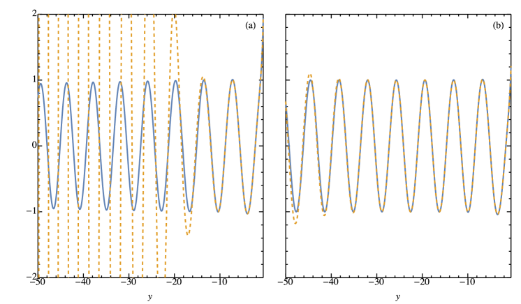
Figure 1: The real part of the exact solution (22) (solid lines) versus that of the approximate expression (32) (dashed lines) as functions of $y\,(=c_{h}k\eta)$. We take (a) $\delta=10^{-2}$ and (b) $\delta=10^{-3}$. It can be seen that the approximation is good for $\delta\times y^{2}\lesssim 1$.

In the next section we compute the 3-point functions by means of the in-in formalism Maldacena:2002vr . To do so, one has to integrate products of $\psi_{\mathbf{k}}$ with respect to time. Unfortunately, this turns out to be impossible in an analytic way if one directly uses $\psi_{\mathbf{k}}$ written in terms of the Whittaker function. Therefore, we assume that the modification to the dispersion relation is small, and expand $\psi_{\mathbf{k}}$ in terms of $\epsilon$. The approximation allows us to calculate the 3-point functions analytically in a perturbative manner.

To second order in $\epsilon$, we find, up to a phase factor,

$$\frac{a{\sqrt{{\cal G}_{T}}}}{2}\psi_{\mathbf{k}}=F(\delta)\frac{e^{-iy+i\delta y^{2}/2}}{\sqrt{2c_{h}k}}\left[-\frac{i}{y}+1-\frac{\delta}{2}\left(y+iy^{2}\right)-\delta^{2}\left(\frac{5}{12}y^{2}+\frac{i}{24}y^{3}+\frac{1}{8}y^{4}\right)+{\cal O}(\delta^{3})\right],$$ (32)

where $y:=c_{h}k\eta$ and $\delta:=\epsilon/c_{h}^{2}$. The approximation is valid as long as $\delta\times y^{2}=\epsilon k^{2}\eta^{2}\lesssim 1$, as is clearly seen from Fig. 1. We use this formula in the following calculations of the 3-point functions of the tensor perturbations. The same approximation was used in Ref. Ashoorioon:2011eg to evaluate the effects of nonstandard dispersion relations on non-Gaussianities of the curvature perturbations.

IV Cubic interactions and 3-point correlation functions

IV.1 The cubic action

Expanding Eq. (10) to third order in $h_{ij}$, we obtain the following cubic action,

$$S = \int\textrm{d}t\textrm{d}^{3}x\,a^{3}\biggl{\{}\frac{c_{3}}{8}\dot{h}_{i}^{j}\dot{h}_{j}^{k}\dot{h}_{k}^{i}+\frac{\mathcal{F}_{T}}{4a^{2}}\left(h_{ik}h_{jl}-\frac{1}{2}h_{ij}h_{kl}\right)h_{ij,kl}+\frac{a_{7}}{8a^{4}}\dot{h}_{k}^{i}\partial^{2}h_{j}^{k}\partial^{2}h_{i}^{j}-\frac{b_{6}}{8a^{2}}\dot{h}_{k}^{i}\dot{h}_{j}^{k}\partial^{2}h_{i}^{j}$$ (33)

$$\qquad\qquad\quad+\frac{\widetilde{d}_{3}}{a^{4}}\partial^{2}h_{ij}\left[\frac{1}{2}h_{ik,l}h_{jl,k}+h_{kl}\left(h_{ik,lj}-\frac{1}{4}h_{kl,ij}-\frac{1}{2}h_{ij,kl}\right)\right]-\frac{d_{7}}{8a^{6}}\partial^{2}h_{i}^{j}\partial^{2}h_{j}^{k}\partial^{2}h_{k}^{i}\biggr{\}}.$$

At this stage, several comments are in order. It is easy to see that $\widetilde{b}_{2}\delta K_{i}^{j}\delta K_{j}^{i}$ does not contribute to the cubic action. It is also noted that $\widetilde{d}_{1}R$ and $\widetilde{a}_{2}R_{i}^{j}\delta K_{j}^{i}$ give rise to the identical terms even at cubic order, leading to the single combination having the coefficient ${\cal F}_{T}$. We are thus left with the above 6 combinations out of the 8 terms in Eq. (10). If the gravitational sector of the theory is described only by the Einstein-Hilbert term, only the terms with the coefficient ${\cal F}_{T}$ remain, and therefore all the other terms signal theories beyond general relativity.

Now let us look at the Horndeski and GLPV subclass by taking $a_{7}=b_{6}=\widetilde{d}_{3}=d_{7}=0$:

$$S\to\int\textrm{d}t\textrm{d}^{3}x\,a^{3}\biggl{[}\frac{c_{3}}{8}\dot{h}_{i}^{j}\dot{h}_{j}^{k}\dot{h}_{k}^{i}+\frac{\mathcal{F}_{T}}{4a^{2}}\left(h_{ik}h_{jl}-\frac{1}{2}h_{ij}h_{kl}\right)h_{ij,kl}\biggr{]}.$$ (34)

As shown in Ref. Gao:2011vs , we have two independent cubic interactions in the Horndeski theory. Those correspond to the two contributions displayed in the above action. We see that no new contributions appear and we have only the above two even in the GLPV theory beyond Horndeski. Thus, we conclude that the tensor bispectrum in the GLPV theory reduces to a combination of the shapes obtained within the Horndeski theory Gao:2011vs .

The other four interaction terms newly appear in Gao’s framework. Among them the $\widetilde{d}_{3}$ and $d_{7}$ terms have also been studied in the context of Hořava gravity Huang:2013epa , though the modification of the mode function due to the nonstandard dispersion relation has been ignored for simplicity. It is worth noting that in the case of the standard dispersion relation, $\widetilde{d}_{3}=0$, the $b_{6}$ term can be recast in the form of the $c_{3}$ term by the use of the linear equation of motion and integration by parts.

IV.2 3-point correlation functions

We turn to evaluate the 3-point correlation functions of the tensor modes. Although some of the 3-point functions have already been obtained in the literature Gao:2011vs ; Huang:2013epa , below we present all the results for completeness. We also evaluate the corrections arising from the nonstandard dispersion relation. Using the in-in formalism Maldacena:2002vr , the 3-point functions can be computed as

$$\langle\widetilde{h}_{i_{1}j_{1}}({\bf k}_{1})\widetilde{h}_{i_{2}j_{2}}({\bf k}_{2})\widetilde{h}_{i_{3}j_{3}}({\bf k}_{3})\rangle=-i\int_{t_{0}}^{t}\textrm{d}t^{\prime}\left\langle\left[\widetilde{h}_{i_{1}j_{1}}(t,{\bf k}_{1})\widetilde{h}_{i_{2}j_{2}}(t,{\bf k}_{2})\widetilde{h}_{i_{3}j_{3}}(t,{\bf k}_{3}),~{}H_{\mathrm{int}}(t^{\prime})\right]\right\rangle,$$ (35)

where $H_{\rm int}$ is the interaction Hamiltonian obtained from the cubic action (33). Actually, integration with respect to time is to be performed using the conformal time rather than $t$ from $\eta=-\infty$ to $\eta=0$. As mentioned earlier, this cannot be done analytically using the exact mode function written in terms of the Whittaker function (22). To make this step feasible, we use instead the approximate expression (32).

For convenience we introduce the non-Gaussian amplitude ${\cal A}_{i_{1}j_{1}i_{2}j_{2}i_{3}j_{3}}$ defined by Gao:2011vs

$$\langle\widetilde{h}_{i_{1}j_{1}}({\bf k}_{1})\widetilde{h}_{i_{2}j_{2}}({\bf k}_{2})\widetilde{h}_{i_{3}j_{3}}({\bf k}_{3})\rangle=(2\pi)^{7}\delta^{(3)}(\mathbf{k}_{1}+\mathbf{k}_{2}+\mathbf{k}_{3})\frac{\mathcal{P}_{h}^{2}}{k_{1}^{3}k_{2}^{3}k_{3}^{3}}\mathcal{A}_{i_{1}j_{1}i_{2}j_{2}i_{3}j_{3}},$$ (36)

where $\mathcal{A}_{i_{1}j_{1}i_{2}j_{2}i_{3}j_{3}}$ is written as a sum of each contribution, which we compute to order $\epsilon^{2}$. It turns out that the corrections due to the nonstandard dispersion relation start at ${\cal O}(\epsilon^{2})$, so that we write

$$\mathcal{A}_{i_{1}j_{1}i_{2}j_{2}i_{3}j_{3}}=\sum_{\bullet=c_{3},a_{7},\cdots}\left(\mathcal{A}^{(\bullet)}_{i_{1}j_{1}i_{2}j_{2}i_{3}j_{3}}+\frac{\epsilon^{2}}{c_{h}^{4}}\mathcal{C}^{(\bullet)}_{i_{1}j_{1}i_{2}j_{2}i_{3}j_{3}}\right),$$ (37)

where $\bullet=c_{3},a_{7},\cdots$ denotes the corresponding term in the cubic action.

First, the non-Gaussian amplitude arising from the cubic interaction with the coefficient ${\cal F}_{T}$ is given by

$${\cal A}_{i_{1}j_{1}i_{2}j_{2}i_{3}j_{3}}^{({\cal F}_{T})} =\widetilde{\cal A}\left\{\Pi_{i_{1}j_{1},ik}({\bf k}_{1})\Pi_{i_{2}j_{2},jl}({\bf k}_{2})\left[k_{3k}k_{3l}\Pi_{i_{3}j_{3},ij}({\bf k}_{3})-\frac{1}{2}k_{3i}k_{3k}\Pi_{i_{3}j_{3},jl}({\bf k}_{3})\right]+\mathrm{5~{}permutations~{}of~{}1,2,3}\right\},$$ (38)

$${\cal C}_{i_{1}j_{1}i_{2}j_{2}i_{3}j_{3}}^{({\cal F}_{T})} =\widetilde{\cal C}\biggl{\{}\Pi_{i_{1}j_{1},ik}({\bf k}_{1})\cdots\biggr{\}},$$ (39)

where in ${\cal C}_{i_{1}j_{1}i_{2}j_{2}i_{3}j_{3}}^{({\cal F}_{T})}$ the structure constructed from $\Pi_{ij,kl}$ is identical to that in ${\cal A}_{i_{1}j_{1}i_{2}j_{2}i_{3}j_{3}}^{({\cal F}_{T})}$ and

$$\widetilde{\mathcal{A}} =\frac{K_{t}}{16}\left(-1+\frac{K_{2}}{K^{2}_{t}}+\frac{K_{3}}{K^{3}_{t}}\right),$$ (40)

$$\widetilde{\cal C} =\frac{K_{t}}{8}\left(1-\frac{K_{2}}{K^{2}_{t}}+3\frac{K_{3}}{K^{3}_{t}}-2\frac{K_{2}^{2}}{K^{4}_{t}}-6\frac{K_{2}K_{3}}{K^{5}_{t}}+6\frac{K_{3}^{2}}{K^{6}_{t}}\right).$$ (41)

Here, we introduced the notations $K_{t}:=k_{1}+k_{2}+k_{3}$, $K_{2}:=k_{1}k_{2}+k_{2}k_{3}+k_{3}k_{1}$, and $K_{3}:=k_{1}k_{2}k_{3}$. Note that ${\cal A}_{i_{1}j_{1}i_{2}j_{2}i_{3}j_{3}}^{({\cal F}_{T})}$ is the only term present in the case of general relativity. Interestingly, this term has the fixed and universal form and is insensitive to an underlying theory and the inflationary energy scale. This result strengthens the statement originally made in the Horndeski theory in Ref. Gao:2011vs .

The concrete expressions for the other amplitudes are obtained as

$$\mathcal{A}^{(c_{3})}_{i_{1}j_{1}i_{2}j_{2}i_{3}j_{3}} =\frac{3c_{3}}{8}\frac{H}{\mathcal{G}_{T}}\cdot\frac{K_{3}^{2}}{K^{3}_{t}}\Pi_{123},$$ (42)

$$\mathcal{A}^{(a_{7})}_{i_{1}j_{1}i_{2}j_{2}i_{3}j_{3}} =\frac{3a_{7}}{8}\frac{H^{3}}{\mathcal{G}_{T}c_{h}^{4}}\cdot\frac{K_{3}^{2}}{K^{3}_{t}}\left(3+4\frac{K_{2}}{K^{2}_{t}}\right)\Pi_{123},$$ (43)

$$\mathcal{A}^{(b_{6})}_{i_{1}j_{1}i_{2}j_{2}i_{3}j_{3}} =-\frac{3b_{6}}{4}\frac{H^{2}}{\mathcal{G}_{T}c_{h}^{2}}\cdot\frac{K_{3}^{2}}{K^{3}_{t}}\Pi_{123},$$ (44)

$$\mathcal{A}^{(d_{7})}_{i_{1}j_{1}i_{2}j_{2}i_{3}j_{3}} =\frac{3d_{7}}{2}\frac{H^{4}}{\mathcal{G}_{T}c_{h}^{6}}\cdot\frac{K_{3}^{2}}{K^{3}_{t}}\left(1+3\frac{K_{2}}{K^{2}_{t}}+15\frac{K_{3}}{K^{3}_{t}}\right)\Pi_{123},$$ (45)

and

$$\mathcal{C}^{(c_{3})}_{i_{1}j_{1}i_{2}j_{2}i_{3}j_{3}} =\mathcal{A}^{(c_{3})}_{i_{1}j_{1}i_{2}j_{2}i_{3}j_{3}}\cdot 2\left(1-12\frac{K_{2}}{K^{2}_{t}}+15\frac{K_{3}}{K^{3}_{t}}\right),$$ (46)

$$\mathcal{C}^{(a_{7})}_{i_{1}j_{1}i_{2}j_{2}i_{3}j_{3}} =\mathcal{A}^{(a_{7})}_{i_{1}j_{1}i_{2}j_{2}i_{3}j_{3}}\cdot 2\left(27-14\frac{K_{2}}{K^{2}_{t}}+30\frac{K_{3}}{K^{3}_{t}}-240\frac{K_{2}^{2}}{K^{4}_{t}}+210\frac{K_{2}K_{3}}{K^{5}_{t}}\right)\left(3+4\frac{K_{2}}{K_{t}^{2}}\right)^{-1},$$ (47)

$$\mathcal{C}^{(b_{6})}_{i_{1}j_{1}i_{2}j_{2}i_{3}j_{3}} =\mathcal{A}^{(b_{6})}_{i_{1}j_{1}i_{2}j_{2}i_{3}j_{3}}\cdot 2\left(7-29\frac{K_{2}}{K^{2}_{t}}+30\frac{K_{3}}{K^{3}_{t}}\right),$$ (48)

$$\mathcal{C}^{(d_{7})}_{i_{1}j_{1}i_{2}j_{2}i_{3}j_{3}} =\mathcal{A}^{(d_{7})}_{i_{1}j_{1}i_{2}j_{2}i_{3}j_{3}}\cdot 20\left(1+3\frac{K_{2}}{K^{2}_{t}}+51\frac{K_{3}}{K^{3}_{t}}-18\frac{K_{2}^{2}}{K^{4}_{t}}-126\frac{K_{2}K_{3}}{K^{5}_{t}}+126\frac{K_{3}^{2}}{K^{6}_{t}}\right)\left(1+3\frac{K_{2}}{K^{2}_{t}}+15\frac{K_{3}}{K^{3}_{t}}\right)^{-1},$$ (49)

where we introduced the shortened notation for the common factor: $\Pi_{123}:=\Pi_{i_{1}j_{1},ij}({\bf k}_{1})\Pi_{i_{2}j_{2},jk}({\bf k}_{2})\Pi_{i_{3}j_{3},ki}({\bf k}_{3})$. We see that ${\cal A}_{i_{1}j_{1}i_{2}j_{2}i_{3}j_{3}}^{(c_{3})}$ and ${\cal A}_{i_{1}j_{1}i_{2}j_{2}i_{3}j_{3}}^{(b_{6})}$ have the same momentum dependences as expected. Finally, the $\widetilde{d}_{3}$ term itself is a small correction of ${\cal O}(\epsilon^{2})$ in our approximation, so that ${\cal A}_{i_{1}j_{1}i_{2}j_{2}i_{3}j_{3}}^{(\widetilde{d}_{3})}=0$ and

$$\mathcal{C}^{(\widetilde{d}_{3})}_{i_{1}j_{1}i_{2}j_{2}i_{3}j_{3}} =\frac{1}{4K_{t}}\left[1+\frac{K_{2}}{K^{2}_{t}}+3\frac{K_{3}}{K^{3}_{t}}\right]\biggl{\{}-k_{3}^{2}\Pi_{i_{3}j_{3},ij}(\mathbf{k}_{3})\biggl{[}\frac{1}{2}\Pi_{i_{2}j_{2},jl}(\mathbf{k}_{2})\Pi_{i_{1}j_{1},ik}(\mathbf{k}_{1})k_{2l}k_{1k}$$

$$\quad+\Pi_{i_{2}j_{2},kl}\left(\Pi_{i_{1}j_{1},ik}k_{1l}k_{1j}-\frac{1}{4}\Pi_{i_{1}j_{1},kl}k_{1i}k_{1j}-\frac{1}{2}\Pi_{i_{1}j_{1},ij}k_{1k}k_{1l}\right)\biggr{]}+\mathrm{5~{}permutations~{}of~{}1,2,3}\bigg{\}}.$$ (50)

Let us investigate the 3-point correlation functions between each polarization mode of gravitational waves. The two polarization modes are expressed as

$$\xi^{(s)}({\bf k})=\tilde{h}_{ij}({\bf k})e_{ij}^{\ast(s)}({\bf k}).$$ (51)

For the 3-point functions $\langle\xi^{(s_{1})}\xi^{(s_{2})}\xi^{(s_{3})}\rangle$ its amplitude can be evaluated by computing

$$\left\{\begin{array}[]{c}\mathcal{A}^{s_{1}s_{2}s_{3}}_{(\bullet)}\\ \mathcal{C}^{s_{1}s_{2}s_{3}}_{(\bullet)}\end{array}\right\}=e_{i_{1}j_{1}}^{\ast(s_{1})}({\bf k}_{1})e_{i_{2}j_{2}}^{\ast(s_{2})}({\bf k}_{2})e_{i_{3}j_{3}}^{\ast(s_{3})}({\bf k}_{3})\times\left\{\begin{array}[]{c}\mathcal{A}_{i_{1}j_{1}i_{2}j_{2}i_{3}j_{3}}^{(\bullet)}\\ \mathcal{C}_{i_{1}j_{1}i_{2}j_{2}i_{3}j_{3}}^{(\bullet)}\end{array}\right\}.$$ (56)

It is straightforward to obtain the following amplitudes,

$$\mathcal{A}^{s_{1}s_{2}s_{3}}_{({\cal F}_{T})} =\widetilde{\mathcal{A}}\cdot F^{s_{1}s_{2}s_{3}}_{({\rm GR})},$$ (57)

$$\mathcal{A}^{s_{1}s_{2}s_{3}}_{(c_{3})} =\frac{3c_{3}}{8}\frac{H}{\mathcal{G}_{T}}\cdot\frac{K_{3}^{2}}{K^{3}_{t}}F^{s_{1}s_{2}s_{3}}_{({\rm H})},$$ (58)

$$\mathcal{A}^{s_{1}s_{2}s_{3}}_{(a_{7})} =\frac{3a_{7}}{8}\frac{H^{3}}{\mathcal{G}_{T}c_{h}^{4}}\cdot\frac{K_{3}^{2}}{K^{3}_{t}}\left(3+4\frac{K_{2}}{K^{2}_{t}}\right)F^{s_{1}s_{2}s_{3}}_{({\rm H})},$$ (59)

$$\mathcal{A}^{s_{1}s_{2}s_{3}}_{(b_{6})} =-\frac{3b_{6}}{4}\frac{H^{2}}{\mathcal{G}_{T}c_{h}^{2}}\cdot\frac{K_{3}^{2}}{K^{3}_{t}}F^{s_{1}s_{2}s_{3}}_{({\rm H})},$$ (60)

$$\mathcal{A}^{s_{1}s_{2}s_{3}}_{(d_{7})} =\frac{3d_{7}}{2}\frac{H^{4}}{\mathcal{G}_{T}c_{h}^{6}}\cdot\frac{K_{3}^{2}}{K^{3}_{t}}\left(1+3\frac{K_{2}}{K^{2}_{t}}+15\frac{K_{3}}{K^{3}_{t}}\right)F^{s_{1}s_{2}s_{3}}_{({\rm H})},$$ (61)

and

$$\mathcal{C}^{s_{1}s_{2}s_{3}}_{{\cal F}_{T}} =\widetilde{\cal C}\cdot F_{({\rm GR})}^{s_{1}s_{2}s_{3}},$$ (62)

$$\mathcal{C}^{s_{1}s_{2}s_{3}}_{(c_{3})} =\mathcal{A}^{s_{1}s_{2}s_{3}}_{(c_{3})}\cdot 2\left(1-12\frac{K_{2}}{K^{2}_{t}}+15\frac{K_{3}}{K^{3}_{t}}\right),$$ (63)

$$\mathcal{C}^{s_{1}s_{2}s_{3}}_{(a_{7})} =\mathcal{A}^{s_{1}s_{2}s_{3}}_{(a_{7})}\cdot 2\left(27-14\frac{K_{2}}{K^{2}_{t}}+30\frac{K_{3}}{K^{3}_{t}}-240\frac{K_{2}^{2}}{K^{4}_{t}}+210\frac{K_{2}K_{3}}{K^{5}_{t}}\right)\left(3+4\frac{K_{2}}{K_{t}^{2}}\right)^{-1},$$ (64)

$$\mathcal{C}^{s_{1}s_{2}s_{3}}_{(b_{6})} =\mathcal{A}^{s_{1}s_{2}s_{3}}_{(b_{6})}\cdot 2\left(7-29\frac{K_{2}}{K^{2}_{t}}+30\frac{K_{3}}{K^{3}_{t}}\right),$$ (65)

$$\mathcal{C}^{s_{1}s_{2}s_{3}}_{(d_{7})} =\mathcal{A}^{s_{1}s_{2}s_{3}}_{(d_{7})}\cdot 20\left(1+3\frac{K_{2}}{K^{2}_{t}}+51\frac{K_{3}}{K^{3}_{t}}-18\frac{K_{2}^{2}}{K^{4}_{t}}-126\frac{K_{2}K_{3}}{K^{5}_{t}}+126\frac{K_{3}^{2}}{K^{6}_{t}}\right)\left(1+3\frac{K_{2}}{K^{2}_{t}}+15\frac{K_{3}}{K^{3}_{t}}\right)^{-1},$$ (66)

$$\mathcal{C}^{s_{1}s_{2}s_{3}}_{(\widetilde{d}_{3})} =\frac{1}{4K_{t}}\left(1+\frac{K_{2}}{K^{2}_{t}}+3\frac{K_{3}}{K^{3}_{t}}\right)F^{s_{1}s_{2}s_{3}}_{(\widetilde{d}_{3})},$$ (67)

where we defined

$$F^{+++}_{({\rm GR})} := \frac{1}{128}\cdot\frac{K^{8}_{t}}{K_{3}^{2}}\left(1-4\frac{K_{2}}{K^{2}_{t}}+8\frac{K_{3}}{K^{3}_{t}}\right),$$ (68)

$$F^{+++}_{({\rm H})} := \frac{1}{64}\cdot\frac{K^{6}_{t}}{K_{3}^{2}}\left(1-4\frac{K_{2}}{K^{2}_{t}}+8\frac{K_{3}}{K^{3}_{t}}\right),$$ (69)

$$F^{+++}_{({\widetilde{d}_{3}})} := \frac{1}{256}\cdot\frac{K^{10}_{t}}{K_{3}^{2}}\left(1-10\frac{K_{2}}{K^{2}_{t}}+28\frac{K_{3}}{K^{3}_{t}}+24\frac{K_{2}^{2}}{K^{4}_{t}}-128\frac{K_{2}K_{3}}{K^{5}_{t}}+160\frac{K_{3}^{2}}{K^{6}_{t}}\right),$$ (70)

and when spins are mixed the corresponding functions can be derived from $F^{++-}_{({\rm GR},{\rm H},\widetilde{d}_{3})}(k_{1},k_{2},k_{3})=F^{+++}_{({\rm GR},{\rm H},\widetilde{d}_{3})}(k_{1},k_{2},-k_{3})$. Note the relations

$$F^{+++}_{({\rm GR})} = \frac{K^{2}_{t}}{2}F^{+++}_{({\rm H})},$$ (71)

$$F^{+++}_{({\widetilde{d}_{3}})} = \frac{K^{10}_{t}}{4}\left(1-6\frac{K_{2}}{K^{2}_{t}}+20\frac{K_{3}}{K^{3}_{t}}\right)F^{+++}_{({\rm H})}.$$ (72)

Since theories in Gao’s framework do not violate the parity symmetry, we have the properties $F^{++-}_{({\rm GR},{\rm H},\widetilde{d}_{3})}=F^{--+}_{({\rm GR},{\rm H},\widetilde{d}_{3})}$ and $F^{---}_{({\rm GR},{\rm H},\widetilde{d}_{3})}=F^{+++}_{({\rm GR},{\rm H},\widetilde{d}_{3})}$. In the equilateral configuration, we have

$$F^{++-}_{({\rm H})}=F^{+-+}_{({\rm H})}=F^{-++}_{({\rm H})}=\frac{1}{9}F^{+++}_{({\rm H})},$$ (73)

$$F^{++-}_{({\rm GR})}=F^{+-+}_{({\rm GR})}=F^{-++}_{({\rm GR})}=\frac{1}{81}F^{+++}_{({\rm GR})},$$ (74)

$$F^{++-}_{(\widetilde{d}_{3})}=F^{+-+}_{(\widetilde{d}_{3})}=F^{-++}_{(\widetilde{d}_{3})}=\frac{13}{189}F^{+++}_{(\widetilde{d}_{3})},$$ (75)

while in the squeezed limit ${\bf k}_{3}\to 0$ we find

$$F_{({\rm GR},\widetilde{d}_{3})}^{+++}\approx F_{({\rm GR},\widetilde{d}_{3})}^{++-}\approx-\frac{k_{1}^{2}}{2},$$ (76)

$$F_{({\rm GR})}^{+-+}\approx F_{({\rm GR})}^{-++}\approx-\frac{k_{3}^{4}}{32k_{1}^{2}},$$ (77)

$$F_{(\widetilde{d}_{3})}^{+-+}\approx F_{(\widetilde{d}_{3})}^{-++}\approx-\frac{7k_{3}^{4}}{32k_{1}^{2}}.$$ (78)

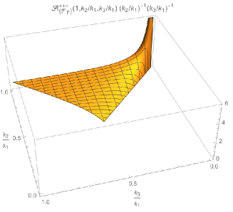
Figure 2: $\mathcal{A}^{+++}_{({\cal F}_{T})}(1,k_{2}/k_{1},k_{3}/k_{1})(k_{2}/k_{1})^{-1}(k_{3}/k_{1})^{-1}$ as a function of $k_{2}/k_{1}$ and $k_{3}/k_{1}$. The plot is normalized to 1 for equilateral configurations $k_{2}/k_{1}=k_{3}/k_{1}=1$.

Figure 3: $\mathcal{A}^{+++}_{(c_{3})}(1,k_{2}/k_{1},k_{3}/k_{1})(k_{2}/k_{1})^{-1}(k_{3}/k_{1})^{-1}$ as a function of $k_{2}/k_{1}$ and $k_{3}/k_{1}$. The plot is normalized to 1 for equilateral configurations $k_{2}/k_{1}=k_{3}/k_{1}=1$.

Figure 4: $\mathcal{A}^{+++}_{(a_{7})}(1,k_{2}/k_{1},k_{3}/k_{1})(k_{2}/k_{1})^{-1}(k_{3}/k_{1})^{-1}$ as a function of $k_{2}/k_{1}$ and $k_{3}/k_{1}$. The plot is normalized to 1 for equilateral configurations $k_{2}/k_{1}=k_{3}/k_{1}=1$.

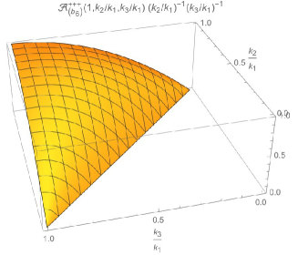
Figure 5: $\mathcal{A}^{+++}_{(b_{6})}(1,k_{2}/k_{1},k_{3}/k_{1})(k_{2}/k_{1})^{-1}(k_{3}/k_{1})^{-1}$ as a function of $k_{2}/k_{1}$ and $k_{3}/k_{1}$. The plot is normalized to 1 for equilateral configurations $k_{2}/k_{1}=k_{3}/k_{1}=1$.

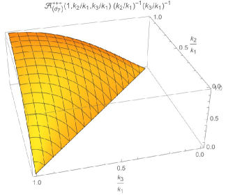
Figure 6: $\mathcal{A}^{+++}_{(d_{7})}(1,k_{2}/k_{1},k_{3}/k_{1})(k_{2}/k_{1})^{-1}(k_{3}/k_{1})^{-1}$ as a function of $k_{2}/k_{1}$ and $k_{3}/k_{1}$. The plot is normalized to 1 for equilateral configurations $k_{2}/k_{1}=k_{3}/k_{1}=1$.

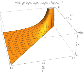
Figure 7: $\mathcal{A}^{++-}_{({\cal F}_{T})}(1,k_{2}/k_{1},k_{3}/k_{1})(k_{2}/k_{1})^{-1}(k_{3}/k_{1})^{-1}$ as a function of $k_{2}/k_{1}$ and $k_{3}/k_{1}$. The plot is normalized to 1 for equilateral configurations $k_{2}/k_{1}=k_{3}/k_{1}=1$.

Figure 8: $\mathcal{A}^{++-}_{(c_{3})}(1,k_{2}/k_{1},k_{3}/k_{1})(k_{2}/k_{1})^{-1}(k_{3}/k_{1})^{-1}$ as a function of $k_{2}/k_{1}$ and $k_{3}/k_{1}$. The plot is normalized to 1 for equilateral configurations $k_{2}/k_{1}=k_{3}/k_{1}=1$.

Figure 9: $\mathcal{A}^{++-}_{(a_{7})}(1,k_{2}/k_{1},k_{3}/k_{1})(k_{2}/k_{1})^{-1}(k_{3}/k_{1})^{-1}$ as a function of $k_{2}/k_{1}$ and $k_{3}/k_{1}$. The plot is normalized to 1 for equilateral configurations $k_{2}/k_{1}=k_{3}/k_{1}=1$.

Figure 10: $\mathcal{A}^{++-}_{(b_{6})}(1,k_{2}/k_{1},k_{3}/k_{1})(k_{2}/k_{1})^{-1}(k_{3}/k_{1})^{-1}$ as a function of $k_{2}/k_{1}$ and $k_{3}/k_{1}$. The plot is normalized to 1 for equilateral configurations $k_{2}/k_{1}=k_{3}/k_{1}=1$.

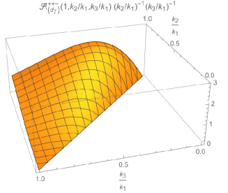
Figure 11: $\mathcal{A}^{++-}_{(d_{7})}(1,k_{2}/k_{1},k_{3}/k_{1})(k_{2}/k_{1})^{-1}(k_{3}/k_{1})^{-1}$ as a function of $k_{2}/k_{1}$ and $k_{3}/k_{1}$. The plot is normalized to 1 for equilateral configurations $k_{2}/k_{1}=k_{3}/k_{1}=1$.

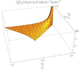
Figure 12: $\mathcal{C}^{+++}_{({\cal F}_{T})}(1,k_{2}/k_{1},k_{3}/k_{1})(k_{2}/k_{1})^{-1}(k_{3}/k_{1})^{-1}$ as a function of $k_{2}/k_{1}$ and $k_{3}/k_{1}$. The plot is normalized to 1 for equilateral configurations $k_{2}/k_{1}=k_{3}/k_{1}=1$.

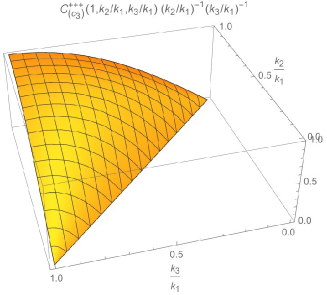
Figure 13: $\mathcal{C}^{+++}_{(c_{3})}(1,k_{2}/k_{1},k_{3}/k_{1})(k_{2}/k_{1})^{-1}(k_{3}/k_{1})^{-1}$ as a function of $k_{2}/k_{1}$ and $k_{3}/k_{1}$. The plot is normalized to 1 for equilateral configurations $k_{2}/k_{1}=k_{3}/k_{1}=1$.

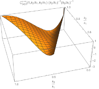
Figure 14: $\mathcal{C}^{+++}_{(a_{7})}(1,k_{2}/k_{1},k_{3}/k_{1})(k_{2}/k_{1})^{-1}(k_{3}/k_{1})^{-1}$ as a function of $k_{2}/k_{1}$ and $k_{3}/k_{1}$. The plot is normalized to 1 for equilateral configurations $k_{2}/k_{1}=k_{3}/k_{1}=1$.

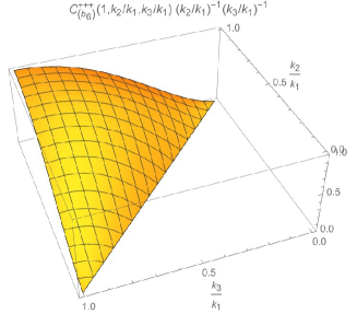
Figure 15: $\mathcal{C}^{+++}_{(b_{6})}(1,k_{2}/k_{1},k_{3}/k_{1})(k_{2}/k_{1})^{-1}(k_{3}/k_{1})^{-1}$ as a function of $k_{2}/k_{1}$ and $k_{3}/k_{1}$. The plot is normalized to 1 for equilateral configurations $k_{2}/k_{1}=k_{3}/k_{1}=1$. .

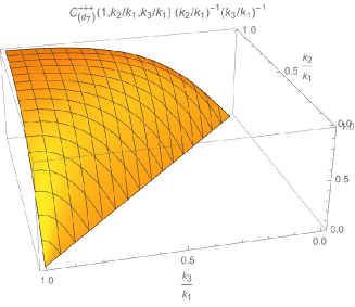
Figure 16: $\mathcal{C}^{+++}_{(d_{7})}(1,k_{2}/k_{1},k_{3}/k_{1})(k_{2}/k_{1})^{-1}(k_{3}/k_{1})^{-1}$ as a function of $k_{2}/k_{1}$ and $k_{3}/k_{1}$. The plot is normalized to 1 for equilateral configurations $k_{2}/k_{1}=k_{3}/k_{1}=1$.

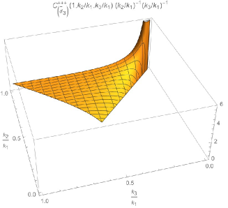
Figure 17: $\mathcal{C}^{+++}_{(\widetilde{d}_{3})}(1,k_{2}/k_{1},k_{3}/k_{1})(k_{2}/k_{1})^{-1}(k_{3}/k_{1})^{-1}$ as a function of $k_{2}/k_{1}$ and $k_{3}/k_{1}$. The plot is normalized to 1 for equilateral configurations $k_{2}/k_{1}=k_{3}/k_{1}=1$.

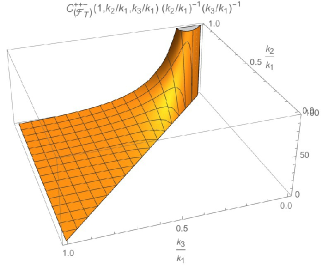
Figure 18: $\mathcal{C}^{++-}_{({\cal F}_{T})}(1,k_{2}/k_{1},k_{3}/k_{1})(k_{2}/k_{1})^{-1}(k_{3}/k_{1})^{-1}$ as a function of $k_{2}/k_{1}$ and $k_{3}/k_{1}$. The plot is normalized to 1 for equilateral configurations $k_{2}/k_{1}=k_{3}/k_{1}=1$.

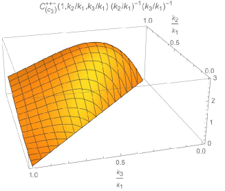
Figure 19: $\mathcal{C}^{++-}_{(c_{3})}(1,k_{2}/k_{1},k_{3}/k_{1})(k_{2}/k_{1})^{-1}(k_{3}/k_{1})^{-1}$ as a function of $k_{2}/k_{1}$ and $k_{3}/k_{1}$. The plot is normalized to 1 for equilateral configurations $k_{2}/k_{1}=k_{3}/k_{1}=1$.

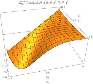
Figure 20: $\mathcal{C}^{++-}_{(a_{7})}(1,k_{2}/k_{1},k_{3}/k_{1})(k_{2}/k_{1})^{-1}(k_{3}/k_{1})^{-1}$ as a function of $k_{2}/k_{1}$ and $k_{3}/k_{1}$. The plot is normalized to 1 for equilateral configurations $k_{2}/k_{1}=k_{3}/k_{1}=1$.

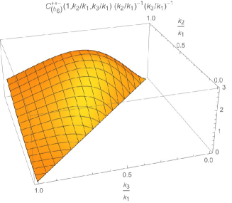
Figure 21: $\mathcal{C}^{++-}_{(b_{6})}(1,k_{2}/k_{1},k_{3}/k_{1})(k_{2}/k_{1})^{-1}(k_{3}/k_{1})^{-1}$ as a function of $k_{2}/k_{1}$ and $k_{3}/k_{1}$. The plot is normalized to 1 for equilateral configurations $k_{2}/k_{1}=k_{3}/k_{1}=1$.

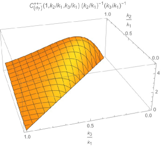
Figure 22: $\mathcal{C}^{++-}_{(d_{7})}(1,k_{2}/k_{1},k_{3}/k_{1})(k_{2}/k_{1})^{-1}(k_{3}/k_{1})^{-1}$ as a function of $k_{2}/k_{1}$ and $k_{3}/k_{1}$. The plot is normalized to 1 for equilateral configurations $k_{2}/k_{1}=k_{3}/k_{1}=1$.

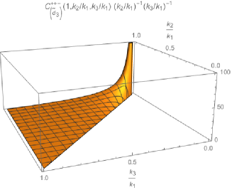
Figure 23: $\mathcal{C}^{++-}_{(\widetilde{d}_{3})}(1,k_{2}/k_{1},k_{3}/k_{1})(k_{2}/k_{1})^{-1}(k_{3}/k_{1})^{-1}$ as a function of $k_{2}/k_{1}$ and $k_{3}/k_{1}$. The plot is normalized to 1 for equilateral configurations $k_{2}/k_{1}=k_{3}/k_{1}=1$.

The configuration dependences of all the “$+++$” and “$++-$” amplitudes and the corresponding ${\cal O}(\epsilon^{2})$ corrections are shown in Figs. 2–23. At leading order in $\epsilon$ expansion, we find that only the contribution from ${\cal F}_{T}$ term, i.e., ${\cal A}_{({\cal F}_{T})}^{+++}$, peaks in the squeezed limit, while all the other ${\cal A}_{(\bullet)}^{+++}$’s peak in the equilateral configuration. We emphasize again that ${\cal A}_{({\cal F}_{T})}^{+++}$ is a fixed and universal feature even for single-field inflation models beyond Horndeski. In other words, it is impossible to suppress or enhance ${\cal A}_{({\cal F}_{T})}^{+++}$ even in the present general framework beyond Horndeski as long as the effect of the modified dispersion relation is small. It would therefore be of great interest to explore this “consistency relation” with CMB B-mode observations such as LiteBIRD Matsumura:2013aja . When spins are mixed, the momentum dependences of ${\cal A}_{(\bullet)}^{++-}\;(\bullet=c_{3},a_{7},b_{6},d_{7})$ are similar to each other and their peaks are located between the equilateral and squeezed configurations. As for the corrections of ${\cal O}(\epsilon^{2})$, it can be seen that they have momentum dependences similar to their leading order counterparts, namely, the relative changes in the amplitudes have mild momentum dependences, as is also the case for the curvature perturbation Ashoorioon:2011eg . However, ${\cal C}_{(\widetilde{d}_{3})}^{+++}$ shows the peak at a squeezed shape, breaking the uniqueness of ${\cal A}_{({\cal F}_{T})}^{+++}$’s momentum dependence at this order. Therefore, it would be interesting to investigate the case where the effect of the modification to the dispersion relation cannot be treated perturbatively.

V Constraints from CMB observations

We can roughly estimate the constraints on the parameters of the theory by comparing the results obtained in the previous section with the Planck results Ade:2015ava ; Ade:2015lrj . Schematically, one has

$$\frac{\langle hhh\rangle}{\langle hh\rangle\langle hh\rangle}\sim\sum\frac{{\cal A}_{(\bullet)}^{s_{1}s_{2}s_{3}}}{k_{1}k_{2}k_{3}}=\sum\frac{{\cal A}_{(\bullet)}^{s_{1}s_{2}s_{3}}(1,k_{2}/k_{1},k_{3}/k_{1})}{(k_{2}/k_{1})(k_{3}/k_{1})},$$ (79)

where the quantities in the right hand side are presented in the previous section. It is reasonable to assume that

$$\langle hhh\rangle\lesssim\langle\mathcal{R}\mathcal{R}\mathcal{R}\rangle,$$ (80)

where ${\cal R}$ is the curvature perturbation. (Otherwise, the dominant source of non-Gaussianity in the CMB comes from the tensor modes, but if so $\langle hhh\rangle$ can be constrained directly from CMB observations.) Then, using the tensor-to-scalar ratio $r=\langle hh\rangle/\langle{\cal R}{\cal R}\rangle$ and the nonlinearity parameters $f_{\rm NL}^{\cal R}$, we have

$$\frac{{\mathcal{A}}_{(\bullet)}^{s_{1}s_{2}s_{3}}}{k_{1}k_{2}k_{3}}\lesssim\frac{\langle\mathcal{R}\mathcal{R}\mathcal{R}\rangle}{\langle hh\rangle\langle hh\rangle}=\frac{1}{r^{2}}\frac{\langle\mathcal{R}\mathcal{R}\mathcal{R}\rangle}{\langle\mathcal{R}\mathcal{R}\rangle\langle\mathcal{R}\mathcal{R}\rangle}\sim\frac{f_{\mathrm{NL}}^{\mathcal{R}}}{r^{2}},$$ (81)

where we have made the second assumption that different ${\mathcal{A}}_{(\bullet)}^{s_{1}s_{2}s_{3}}$’s do not cancel each other. Thus, we obtain the constraint

$$\frac{{\mathcal{A}}_{(\bullet)}^{s_{1}s_{2}s_{3}}}{k_{1}k_{2}k_{3}}\lesssim\frac{f_{\mathrm{NL}}^{\mathcal{R}}}{r^{2}}\sim 10^{3}\left(\frac{r}{0.1}\right)^{-2}\left(\frac{f_{\mathrm{NL}}^{\mathcal{R}}}{10}\right),$$ (82)

which is translated to

$$\frac{c_{3}H}{{\cal G}_{T}},\;\frac{a_{7}H^{3}}{{\cal G}_{T}c_{h}^{4}},\;\frac{b_{6}H^{2}}{{\cal G}_{T}c_{h}^{2}},\;\frac{d_{7}H^{4}}{{\cal G}_{T}c_{h}^{6}}\lesssim 10^{3}\left(\frac{r}{0.1}\right)^{-2}\left(\frac{f_{\mathrm{NL}}^{\mathcal{R}}}{10}\right),$$ (83)

or, equivalently,

$$\frac{c_{3}c_{h}}{H},\;\frac{a_{7}H}{c_{h}^{3}},\;\frac{b_{6}}{c_{h}},\;\frac{d_{7}H^{2}}{c_{h}^{5}}\lesssim 10^{13}\left(\frac{r}{0.1}\right)^{-3}\left(\frac{{\cal P}_{\cal R}}{10^{-9}}\right)^{-1}\left(\frac{f_{\mathrm{NL}}^{\mathcal{R}}}{10}\right),$$ (84)

where ${\cal P}_{\cal R}$ is the power spectrum of the curvature perturbation. Note the mass dimensions of the coefficients: $[c_{3}]=1,~{}[b_{6}]=0,~{}[a_{7}]=-1,$ and $[d_{7}]=-2$. Thus, the current constraints are very weak.

VI Discussions and Conclusions

In this paper, we have clarified primordial non-Gaussianities of tensor modes by computing the tensor 3-point functions within the unifying framework of scalar-tensor theories Gao:2014soa . The framework includes the Horndeski theory and recent GLPV generalization as specific cases. We have shown that no new terms appear in the cubic Lagrangian even if one goes to the GLPV theory beyond Horndeski. In more general theories beyond GLPV, we have found four new interactions, one of which is related to the modification of the dispersion relation in the linear theory. The impact of this modification of the dispersion relation can be parametrized using a small parameter $\epsilon$, and we have computed the 3-point functions analytically by treating $\epsilon$ as a small expansion parameter. Two of the four new terms beyond GLPV have already been studied to leading order in $\epsilon$ in the context of Hořava gravity Huang:2013epa , and our results are in agreement with those in Ref. Huang:2013epa where they overlap. In Ref. Gao:2011vs it was found that there are only two independent terms in the cubic Lagrangian within Horndeski: the standard one present already in general relativity generating squeezed non-Gaussianity with the fixed amplitude and the other nonstandard one predicting equilateral non-Gaussianity. We have strengthened this statement by showing that at leading order in the $\epsilon$ expansion the squeezed non-Gaussianity is only generated by this “standard” cubic term and has the fixed amplitude, ${\cal A}_{({\cal F}_{T})}^{+++}$, even in the general unifying framework of scalar-tensor theories. At leading order in $\epsilon$ all the other non-Gaussian amplitudes peak at equilateral shapes. The “standard” interaction is quite likely to be present in the cubic Lagrangian because it can easily be generated from the term linear in the Ricci scalar. The fixed and universal nature of ${\cal A}_{({\cal F}_{T})}^{+++}$ thus provides us the “consistency relation” in the primordial tensor sector. Any detection of the equilateral tensor non-Gaussianity would imply the nonstandard interactions between gravity and the scalar degree of freedom, though it is difficult to distinguish among different contributions. Note that the inverse is not true; even in the absence of equilateral non-Gaussianity, gravity could be modified significantly from general relativity, because one can consider various nonstandard interactions that do not affect the tensor sector, as well as $R_{i}^{j}\delta K_{j}^{i}$.

We have found that the effects of the modified dispersion relation appear in the non-Gaussian amplitudes at ${\cal O}(\epsilon^{2})$. The momentum dependences of the correction $\mathcal{C}_{(\bullet)}^{s_{1}s_{2}s_{3}}$ are similar to their leading order counterparts $\mathcal{A}_{(\bullet)}^{s_{1}s_{2}s_{3}}$. It should be noted that the correction to the squeezed non-Gaussianity, $\mathcal{C}_{({\cal F}_{T})}^{s_{1}s_{2}s_{3}}$, breaks its fixed and universal nature. Therefore, detection of squeezed tensor non-Gaussianity whose amplitude is different from ${\cal A}_{({\cal F}_{T})}^{+++}$ would imply a significant higher order term in the dispersion relation or the tensor modes of non-inflationary origin.

Let us mention here some other sources of gravitational waves from the early universe, as it would be interesting to explore tensor non-Gaussian signatures of such origin in order to contrast them with the results in this paper. A spectator scalar field other than inflaton can produce gravitational waves Biagetti:2013kwa , though it is difficult to expect large amplitudes Biagetti:2014asa ; Fujita:2014oba . Large tensor modes are produced, e.g., by self-ordering of multi-component scalar fields after a global phase transition JonesSmith:2007ne ; Fenu:2009qf ; Giblin:2011yh ; Figueroa:2012kw ; Kuroyanagi:2015esa . Vector fields can also source gravitational waves during inflation Mukohyama:2014gba ; Barnaby:2010vf . We hope that we will come back to the issue of non-Gaussian signatures of those gravitational waves in future publications.

Finally, it should be noted that by construction the present analysis does not cover multi-field inflation models. Though the multi-field effects in the tensor sector are expected to be small, it would be interesting to investigate whether one can discriminate single- and multi-field models using primordial non-Gaussianity of tensor modes.

Appendix A Disformal transformation

Let us investigate the transformation properties of the quadratic and cubic actions under the disformal transformation,

$$\hat{g}_{\mu\nu}=A(\phi,X)g_{\mu\nu}+B(\phi,X)\partial_{\mu}\phi\partial_{\nu}\phi.$$ (85)

It is more convenient to write this in the unitary gauge as

$$\hat{g}_{\mu\nu}=e^{2\alpha}\left[g_{\mu\nu}+\left(1-e^{2\beta}\right)n_{\mu}n_{\nu}\right],$$ (86)

where $n_{\mu}$ is the unit normal to the constant time hypersurfaces, $n_{\mu}=(-N,0)$. Since we are interested in the tensor perturbations on a cosmological background, we may only consider the case where both $\alpha$ and $\beta$ are functions of time and do not fluctuate. Under the above disformal transformation, the ADM variables transform as

$$\hat{\gamma}_{ij}=e^{2\alpha}\gamma_{ij},\quad\hat{N}=e^{\alpha+\beta}N,\quad\hat{N}^{i}=N^{i},$$ (87)

yielding

$$\hat{K}_{i}^{j} =e^{-\alpha-\beta}\left(K_{i}^{j}+\frac{\dot{\alpha}}{N}\delta_{i}^{j}\right),$$ (88)

$$\hat{R}_{i}^{j} =e^{-2\alpha}R_{i}^{j}.$$ (89)

Substituting these to the Lagrangian (10), we find that the disformal transformation maintains the form of the Lagrangian for the tensor perturbations:

$$\frac{{\cal L}}{\sqrt{-g}}\to\frac{{\cal L}}{\sqrt{-\hat{g}}} = \hat{d}_{1}\hat{R}+\hat{d}_{3}\hat{R}_{i}^{j}\hat{R}_{j}^{i}+\hat{d}_{7}\hat{R}_{i}^{j}\hat{R}_{j}^{k}\hat{R}_{k}^{i}+\hat{b}_{2}\hat{\delta K}_{i}^{j}\hat{\delta K}_{j}^{i}+\hat{c}_{3}\hat{\delta K}_{i}^{j}\hat{\delta K}_{j}^{k}\hat{\delta K}_{k}^{i}$$ (90)

$$+\hat{a}_{2}\hat{R}_{i}^{j}\hat{\delta K}_{j}^{i}+\hat{a}_{7}\hat{R}_{i}^{j}\hat{R}_{j}^{k}\hat{\delta K}_{k}^{i}+\hat{b}_{6}\hat{R}_{i}^{j}\hat{\delta K}_{j}^{k}\hat{\delta K}_{k}^{i},$$

where

$$\hat{d}_{1}=e^{-2\alpha-\beta}\widetilde{d}_{1},\quad\hat{d}_{3}=e^{-\beta}\widetilde{d}_{3},\quad\hat{d}_{7}=e^{2\alpha-\beta}d_{7},\quad\hat{b}_{2}=e^{-2\alpha+\beta}b_{2},$$

$$\hat{c}_{3}=e^{-\alpha+2\beta}c_{3},\quad\hat{a}_{2}=e^{-\alpha}\widetilde{a}_{2},\quad\hat{a}_{7}=e^{\alpha}a_{7},\quad\hat{b}_{6}=e^{\beta}b_{6},$$ (91)

and we dropped the terms that are irrelevant to the tensor perturbations. This, in particular, implies that

$${\cal G}_{T}\to\hat{\cal G}_{T}=e^{-2\alpha+\beta}{\cal G}_{T},\quad{\cal F}_{T}\to\hat{\cal F}_{T}=e^{-2\alpha-\beta}{\cal F}_{T}.$$ (92)

Using the two time-dependent functions $\alpha$ and $\beta$, one can fit ${\cal G}_{T}$ and ${\cal F}_{T}$ to the standard form, i.e., $\hat{\cal G}_{T}=\hat{\cal F}_{T}=M_{\textrm{Pl}}^{2}$ Creminelli:2014wna . However, the higher order term in the dispersion relation cannot be removed Fujita:2015ymn . It is also clear that one cannot make further simplifications in the cubic action by the use of the disformal transformation.

References

• (1) A. H. Guth, “The Inflationary Universe: A Possible Solution to the Horizon and Flatness Problems,” Phys. Rev. D 23, 347 (1981). doi:10.1103/PhysRevD.23.347
• (2) K. Sato, “First Order Phase Transition of a Vacuum and Expansion of the Universe,” Mon. Not. Roy. Astron. Soc.  195, 467 (1981).
• (3) A. A. Starobinsky, “A New Type of Isotropic Cosmological Models Without Singularity,” Phys. Lett. B 91, 99 (1980). doi:10.1016/0370-2693(80)90670-X
• (4) P. A. R. Ade et al. [Planck Collaboration], “Planck 2015 results. XX. Constraints on inflation,” arXiv:1502.02114 [astro-ph.CO].
• (5) X. Chen, M. x. Huang, S. Kachru and G. Shiu, “Observational signatures and non-Gaussianities of general single field inflation,” JCAP 0701, 002 (2007) [hep-th/0605045].
• (6) P. A. R. Ade et al. [Planck Collaboration], “Planck 2015 results. XVII. Constraints on primordial non-Gaussianity,” arXiv:1502.01592 [astro-ph.CO].
• (7) J. M. Maldacena, “Non-Gaussian features of primordial fluctuations in single field inflationary models,” JHEP 0305, 013 (2003) [astro-ph/0210603].
• (8) J. M. Maldacena and G. L. Pimentel, “On graviton non-Gaussianities during inflation,” JHEP 1109, 045 (2011) [arXiv:1104.2846 [hep-th]].
• (9) J. Soda, H. Kodama and M. Nozawa, “Parity Violation in Graviton Non-gaussianity,” JHEP 1108, 067 (2011) [arXiv:1106.3228 [hep-th]].
• (10) P. McFadden and K. Skenderis, “Cosmological 3-point correlators from holography,” JCAP 1106, 030 (2011) [arXiv:1104.3894[hep-th]].
• (11) X. Gao, T. Kobayashi, M. Yamaguchi and J. Yokoyama, “Primordial non-Gaussianities of gravitational waves in the most general single-field inflation model,” Phys. Rev. Lett.  107, 211301 (2011) [arXiv:1108.3513 [astro-ph.CO]].
• (12) X. Gao, T. Kobayashi, M. Shiraishi, M. Yamaguchi, J. Yokoyama and S. Yokoyama, “Full bispectra from primordial scalar and tensor perturbations in the most general single-field inflation model,” PTEP 2013, 053E03 (2013) [arXiv:1207.0588 [astro-ph.CO]].
• (13) Y. Huang, A. Wang, R. Yousefi and T. Zhu, “Primordial non-Gaussianity of gravitational waves in Hořava-Lifshitz gravity,” Phys. Rev. D 88, no. 2, 023523 (2013) [arXiv:1304.1556 [hep-th]].
• (14) A. Bzowski, P. McFadden and K. Skenderis, “Holographic predictions for cosmological 3-point functions,” JHEP 1203, 091 (2012) doi:10.1007/JHEP03(2012)091 [arXiv:1112.1967 [hep-th]].
• (15) T. Zhu, W. Zhao, Y. Huang, A. Wang and Q. Wu, “Effects of parity violation on non-gaussianity of primordial gravitational waves in Hořava-Lifshitz gravity,” Phys. Rev. D 88, 063508 (2013) doi:10.1103/PhysRevD.88.063508 [arXiv:1305.0600 [hep-th]].
• (16) J. L. Cook and L. Sorbo, “An inflationary model with small scalar and large tensor nongaussianities,” JCAP 1311, 047 (2013) doi:10.1088/1475-7516/2013/11/047 [arXiv:1307.7077 [astro-ph.CO]].
• (17) V. Sreenath, R. Tibrewala and L. Sriramkumar, “Numerical evaluation of the three-point scalar-tensor cross-correlations and the tensor bi-spectrum,” JCAP 1312, 037 (2013) doi:10.1088/1475-7516/2013/12/037 [arXiv:1309.7169 [astro-ph.CO]].
• (18) T. Noumi and M. Yamaguchi, “Non-Gaussianities of primordial perturbations and tensor sound speed,” arXiv:1403.6065 [hep-th].
• (19) V. Sreenath and L. Sriramkumar, “Examining the consistency relations describing the three-point functions involving tensors,” JCAP 1410, no. 10, 021 (2014) doi:10.1088/1475-7516/2014/10/021 [arXiv:1406.1609 [astro-ph.CO]].
• (20) T. F. Fu and Q. G. Huang, “The four-point correlation function of graviton during inflation,” JHEP 1507, 132 (2015) doi:10.1007/JHEP07(2015)132 [arXiv:1502.02329 [hep-th]].
• (21) D. Chowdhury, V. Sreenath and L. Sriramkumar, “The tensor bi-spectrum in a matter bounce,” JCAP 1511, no. 11, 002 (2015) doi:10.1088/1475-7516/2015/11/002 [arXiv:1506.06475 [astro-ph.CO]].
• (22) T. Kobayashi, M. Yamaguchi and J. Yokoyama, “Generalized G-inflation: Inflation with the most general second-order field equations,” Prog. Theor. Phys.  126, 511 (2011) [arXiv:1106.0723 [hep-th]].
• (23) G. W. Horndeski, “Second-order scalar-tensor field equations in a four-dimensional space,” Int. J. Theor. Phys.  10, 363 (1974).
• (24) C. Deffayet, X. Gao, D. A. Steer and G. Zahariade, “From k-essence to generalised Galileons,” Phys. Rev. D 84, 064039 (2011) [arXiv:1103.3260 [hep-th]].
• (25) X. Gao and D. A. Steer, “Inflation and primordial non-Gaussianities of ’generalized Galileons’,” JCAP 1112, 019 (2011) doi:10.1088/1475-7516/2011/12/019 [arXiv:1107.2642 [astro-ph.CO]].
• (26) A. De Felice and S. Tsujikawa, “Inflationary non-Gaussianities in the most general second-order scalar-tensor theories,” Phys. Rev. D 84, 083504 (2011) doi:10.1103/PhysRevD.84.083504 [arXiv:1107.3917 [gr-qc]].
• (27) S. Renaux-Petel, “On the redundancy of operators and the bispectrum in the most general second-order scalar-tensor theory,” JCAP 1202, 020 (2012) doi:10.1088/1475-7516/2012/02/020 [arXiv:1107.5020 [astro-ph.CO]].
• (28) R. H. Ribeiro and D. Seery, “Decoding the bispectrum of single-field inflation,” JCAP 1110, 027 (2011) doi:10.1088/1475-7516/2011/10/027 [arXiv:1108.3839 [astro-ph.CO]].
• (29) A. De Felice and S. Tsujikawa, “Shapes of primordial non-Gaussianities in the Horndeski’s most general scalar-tensor theories,” JCAP 1303, 030 (2013) doi:10.1088/1475-7516/2013/03/030 [arXiv:1301.5721 [hep-th]].
• (30) J. Gleyzes, D. Langlois, F. Piazza and F. Vernizzi, “Healthy theories beyond Horndeski,” Phys. Rev. Lett.  114, no. 21, 211101 (2015) [arXiv:1404.6495 [hep-th]].
• (31) J. Gleyzes, D. Langlois, F. Piazza and F. Vernizzi, “Exploring gravitational theories beyond Horndeski,” JCAP 1502, 018 (2015) [arXiv:1408.1952 [astro-ph.CO]].
• (32) X. Gao, “Unifying framework for scalar-tensor theories of gravity,” Phys. Rev. D 90, no. 8, 081501 (2014) [arXiv:1406.0822 [gr-qc]].
• (33) R. Kase and S. Tsujikawa, “Effective field theory approach to modified gravity including Horndeski theory and Hořava-Lifshitz gravity,” Int. J. Mod. Phys. D 23, no. 13, 1443008 (2015) doi:10.1142/S0218271814430081 [arXiv:1409.1984 [hep-th]].
• (34) A. De Felice and S. Tsujikawa, “Inflationary gravitational waves in the effective field theory of modified gravity,” Phys. Rev. D 91, no. 10, 103506 (2015) doi:10.1103/PhysRevD.91.103506 [arXiv:1411.0736 [hep-th]].
• (35) A. De Felice, K. Koyama and S. Tsujikawa, “Observational signatures of the theories beyond Horndeski,” JCAP 1505, no. 05, 058 (2015) doi:10.1088/1475-7516/2015/05/058 [arXiv:1503.06539 [gr-qc]].
• (36) T. Fujita, X. Gao and J. Yokoyama, “Spatially covariant theories of gravity: disformal transformation, cosmological perturbations and the Einstein frame,” arXiv:1511.04324 [gr-qc].
• (37) M. Fasiello and S. Renaux-Petel, “Non-Gaussian inflationary shapes in $G^{3}$ theories beyond Horndeski,” JCAP 1410, no. 10, 037 (2014) doi:10.1088/1475-7516/2014/10/037 [arXiv:1407.7280 [astro-ph.CO]].
• (38) C. Lin, S. Mukohyama, R. Namba and R. Saitou, “Hamiltonian structure of scalar-tensor theories beyond Horndeski,” JCAP 1410, no. 10, 071 (2014) [arXiv:1408.0670 [hep-th]].
• (39) C. Deffayet, G. Esposito-Farese and D. A. Steer, “Counting the degrees of freedom of generalized Galileons,” Phys. Rev. D 92, 084013 (2015) [arXiv:1506.01974 [gr-qc]].
• (40) D. Langlois and K. Noui, “Degenerate higher derivative theories beyond Horndeski: evading the Ostrogradski instability,” arXiv:1510.06930 [gr-qc].
• (41) M. Zumalacárregui and J. García-Bellido, “Transforming gravity: from derivative couplings to matter to second-order scalar-tensor theories beyond the Horndeski Lagrangian,” Phys. Rev. D 89, 064046 (2014) doi:10.1103/PhysRevD.89.064046 [arXiv:1308.4685 [gr-qc]].
• (42) S. Ohashi, N. Tanahashi, T. Kobayashi and M. Yamaguchi, “The most general second-order field equations of bi-scalar-tensor theory in four dimensions,” JHEP 1507, 008 (2015) doi:10.1007/JHEP07(2015)008 [arXiv:1505.06029 [gr-qc]].
• (43) X. Gao, “Hamiltonian analysis of spatially covariant gravity,” Phys. Rev. D 90, no. 10, 104033 (2014) [arXiv:1409.6708 [gr-qc]].
• (44) P. Hořva, “Quantum Gravity at a Lifshitz Point,” Phys. Rev. D 79, 084008 (2009) [arXiv:0901.3775 [hep-th]].
• (45) D. Blas, O. Pujolas and S. Sibiryakov, “Consistent Extension of Hořva Gravity,” Phys. Rev. Lett.  104, 181302 (2010) [arXiv:0909.3525 [hep-th]].
• (46) A. Ashoorioon, D. Chialva and U. Danielsson, “Effects of Nonlinear Dispersion Relations on Non-Gaussianities,” JCAP 1106, 034 (2011) [arXiv:1104.2338 [hep-th]].
• (47) J. Martin and R. H. Brandenberger, “The Corley-Jacobson dispersion relation and transPlanckian inflation,” Phys. Rev. D 65, 103514 (2002) [hep-th/0201189].
• (48) T. Kobayashi, M. Yamaguchi and J. Yokoyama, “Galilean Creation of the Inflationary Universe,” JCAP 1507, no. 07, 017 (2015) [arXiv:1504.05710 [hep-th]].
• (49) T. Matsumura et al., “Mission design of LiteBIRD,” Journal of Low Temperature Physics September 2014, Volume 176, Issue 5-6, pp 733-740 doi:10.1007/s10909-013-0996-1 [arXiv:1311.2847 [astro-ph.IM]].
• (50) N. Arkani-Hamed, P. Creminelli, S. Mukohyama and M. Zaldarriaga, “Ghost inflation,” JCAP 0404, 001 (2004) doi:10.1088/1475-7516/2004/04/001 [hep-th/0312100].
• (51) M. Biagetti, M. Fasiello and A. Riotto, “Enhancing Inflationary Tensor Modes through Spectator Fields,” Phys. Rev. D 88, 103518 (2013) [arXiv:1305.7241 [astro-ph.CO]].
• (52) M. Biagetti, E. Dimastrogiovanni, M. Fasiello and M. Peloso, “Gravitational Waves and Scalar Perturbations from Spectator Fields,” JCAP 1504, 011 (2015) doi:10.1088/1475-7516/2015/04/011 [arXiv:1411.3029 [astro-ph.CO]].
• (53) T. Fujita, J. Yokoyama and S. Yokoyama, “Can a spectator scalar field enhance inflationary tensor mode?,” PTEP 2015, 043E01 (2015) [arXiv:1411.3658 [astro-ph.CO]].
• (54) K. Jones-Smith, L. M. Krauss and H. Mathur, “A Nearly Scale Invariant Spectrum of Gravitational Radiation from Global Phase Transitions,” Phys. Rev. Lett.  100, 131302 (2008) doi:10.1103/PhysRevLett.100.131302 [arXiv:0712.0778 [astro-ph]].
• (55) E. Fenu, D. G. Figueroa, R. Durrer and J. Garcia-Bellido, “Gravitational waves from self-ordering scalar fields,” JCAP 0910, 005 (2009) doi:10.1088/1475-7516/2009/10/005 [arXiv:0908.0425 [astro-ph.CO]].
• (56) J. T. Giblin, Jr., L. R. Price, X. Siemens and B. Vlcek, “Gravitational Waves from Global Second Order Phase Transitions,” JCAP 1211, 006 (2012) doi:10.1088/1475-7516/2012/11/006 [arXiv:1111.4014 [astro-ph.CO]].
• (57) D. G. Figueroa, M. Hindmarsh and J. Urrestilla, “Exact Scale-Invariant Background of Gravitational Waves from Cosmic Defects,” Phys. Rev. Lett.  110, no. 10, 101302 (2013) doi:10.1103/PhysRevLett.110.101302 [arXiv:1212.5458 [astro-ph.CO]].
• (58) S. Kuroyanagi, T. Hiramatsu and J. Yokoyama, “Reheating signature in the gravitational wave spectrum from self-ordering scalar fields,” arXiv:1509.08264 [astro-ph.CO].
• (59) S. Mukohyama, R. Namba, M. Peloso and G. Shiu, “Blue Tensor Spectrum from Particle Production during Inflation,” JCAP 1408, 036 (2014) [arXiv:1405.0346 [astro-ph.CO]].
• (60) N. Barnaby and M. Peloso, “Large Nongaussianity in Axion Inflation,” Phys. Rev. Lett.  106, 181301 (2011) [arXiv:1011.1500 [hep-ph]].
• (61) P. Creminelli, J. Gleyzes, J. Noreña and F. Vernizzi, “Resilience of the standard predictions for primordial tensor modes,” Phys. Rev. Lett.  113, no. 23, 231301 (2014) doi:10.1103/PhysRevLett.113.231301 [arXiv:1407.8439 [astro-ph.CO]].