Dissipation enabled efficient excitation transfer from a single photon to a single quantum emitter

Abstract

We propose a scheme for triggering a dissipation dominated highly efficient excitation transfer from a single photon wave packet to a single quantum emitter. This single photon induced optical pumping turns dominant dissipative processes, such as spontaneous photon emission by the emitter or cavity decay, into valuable tools for quantum information processing and quantum communication. It works for an arbitrarily shaped single photon wave packet with sufficiently small bandwidth provided a matching condition is satisfied which balances the dissipative rates involved. Our scheme does not require additional laser pulses or quantum feedback and does not rely on high finesse optical resonators. In particular, it can be used to enhance significantly the coupling of a single photon to a single quantum emitter implanted in a one dimensional waveguide or even in a free space scenario. We demonstrate the usefulness of our scheme for building a deterministic quantum memory and a deterministic frequency converter between photonic qubits of different wavelengths.

I Introduction

Achieving highly efficient excitation transfer from a single photon to a material quantum system with the possibility of a controlled manipulation of the resulting quantum state is a crucial prerequisite for advancing quantum technology with potential applications ranging from quantum communication Kimble and computation Nielsen to fundamental tests of quantum mechanics hensen2015experimental . Coherent quantum processes provide powerful tools for such an excitation transfer on the single photon level.

With the help of electromagnetically induced transparency fleischhauer2000dark ; phillips2001storage , for example, a single photon wave packet of quite arbitrary pulse shape can be stored in a collective excitation of a macroscopically large number of atoms phillips2001storage or in a solid de2008solid . However, the controlled manipulation of the resulting macroscopic excitation for purposes of quantum information processing is highly challenging. In contrast, excitation transfer from a single photon to a single quantum emitter, such as a trapped atom, offers the advantage that the resulting quantum state can be manipulated with high accuracy Cirac1997 ; Ritter ; duan2004scalable ; reiserer2013nondestructive ; reiserer2014quantum ; kalb2015heralded . Based on coherent processes an early protocol suitable for scalable photonic quantum information processing has been proposed by Cirac et al. Cirac1997 and has been implemented experimentally by Ritter et al.Ritter . However, this protocol requires detailed knowledge of shape and of arrival time of the photon wave packet for triggering an appropriate coherent laser-induced process. A coherent scheme overcoming the complications of such a conditional pulse shaping has been proposed by Duan and Kimble duan2004scalable . It takes advantage of a trapped atom’s state dependent frequency shift of the cavity mode which results in a phase flip of an incoming single photon reflected by the cavity. This scheme has been used to build a nondestructive photon detector reiserer2013nondestructive , a quantum gate between a matter and a photonic qubit reiserer2014quantum , and a quantum memory for the heralded storage of a single photonic qubit kalb2015heralded . However, for the heralded storage of a single photonic qubit the outgoing photon has to be measured and quantum feedback has to be applied. Thus, the efficiency is limited by the efficiency of the single photon detector.

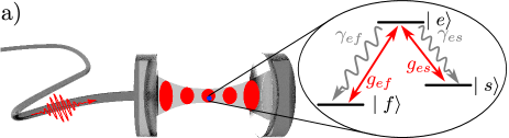
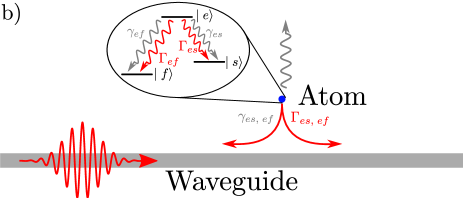
Figure 1: (a): Schematic representation of a fiber and cavity based scenario. A single three level atom is trapped inside the cavity and a single photon is propagating through the fiber. (b): Schematic representation of a three level atom coupled to the evanescent field surrounding a one dimensional waveguide with a single photon propagating along this waveguide.

The natural question arises whether it is possible to achieve highly efficient excitation transfer from a single photon with a rather arbitrary pulse shape to a single quantum emitter also in a way that the challenging complications arising from conditional tailoring of laser pulses and from imperfections affecting postselective photon detection processes can be circumvented. We present such a scheme which is capable of accomplishing basic tasks of quantum information processing, such as implementing a deterministic single atom quantum memory or a deterministic frequency converter for a photonic qubit. Contrary to previous proposals based on coherent quantum processes our scheme is enabled by an appropriate balancing of dissipative processes, such as spontaneous photon emission and cavity decay. It is demonstrated that this way a single photon wave packet of rather arbitrary shape can trigger a highly efficient excitation transfer to a material quantum emitter. For photon wave packets with sufficiently small bandwidths the high efficiency of this excitation transfer is independent of the photon wave packet’s shape.

This single photon induced optical pumping happer1972optical does not require an optical resonator and is applicable to various scenarios including highly efficient coupling of a single atom to a single photon propagating in a one dimensional waveguide, such as a nanowire akimov2007generation ; schuller2010plasmonics , or a nanofiber vetsch2010optical , or in a coplanar waveguide (circuit QED) you2011atomic , or even in free space maiwald2012collecting ; fischer2014efficient . A schematic representation of a suitable cavity and fiber based scenario as well as a schematic representation of an atom coupled to the evanescent field surrounding a one dimensional waveguide is depicted in Fig. 1 (a) and (b).

The scheme presented in this article paves the way to scalable quantum communication networks, as it relaxes the requirements on the synchronization of the nodes of the network, i.e. detailed knowledge on the arrival time and shape of the photons is not required, and it is not limited by the efficiency of single photon detectors.

The body of this article is divided into four parts. In Sec. II we introduce the Hamiltonians for modeling the dynamics for a fiber and cavity based scenario as well as for a waveguide or free space scenario. Based on these models, we analyze the dynamics of these systems in Sec. III, and derive the conditions for triggering an efficient excitation transfer. A key step in the derivation of these analytical results is an adiabatic approximation. In Sec. IV, we supplement these analytical results by a numerical investigation. We show that our scheme allows to trigger an efficient state transfer also with photons of a finite bandwidth. Finally, in Sec. V we show possible application of our scheme for building a deterministic quantum memory and a deterministic frequency converter between photonic qubits of different wavelengths.

II Quantum optical model

Let us start by considering a fiber and cavity based system as schematically depicted in Fig. 1 (a). A three level atom is interacting resonantly with two modes of a surrounding high finesse cavity. A photon propagating through a fiber can enter this cavity by transmission through a mirror of the single-sided cavity. Spontaneous decay of the three level atom is modeled by coupling to the continua of electromagnetic field modes orthogonal to the modes of the resonant cavity and of the fiber. We assume that the dipole and rotating wave approximations are applicable. In the interaction picture the Hamiltonian reads

$$\hat{H}_{\text{int}}^{\text{cavity}}(t)/\hbar = \left[ig_{es}\hat{a}_{es}^{\text{C}\dagger}\mid s\rangle\langle e\mid+ig_{ef}\hat{a}_{ef}^{\text{C}\dagger}\mid f\rangle\langle e\mid+\text{H.c.}\right]$$

$$+\left[\sqrt{2\kappa_{es}}\hat{a}^{\text{F}_{es}}(t)\hat{a}_{es}^{\text{C}\dagger}+\text{H.c.}\right]$$

$$+\left[\sqrt{2\kappa_{ef}}\hat{a}^{\text{F}_{ef}}(t)\hat{a}_{ef}^{\text{C}\dagger}+\text{H.c.}\right]$$

$$-\frac{1}{\hbar}\left[e^{-i\omega_{es}\left(t-t_{0}\right)}\mathbf{d}_{es}\cdot\hat{\mathbf{E}}_{\text{B}_{es}}^{-}(t)\mid s\rangle\langle e\mid+\text{H.c.}\right]$$

$$-\frac{1}{\hbar}\left[e^{-i\omega_{ef}\left(t-t_{0}\right)}\mathbf{d}_{ef}\cdot\hat{\mathbf{E}}_{\text{B}_{ef}}^{-}(t)\mid f\rangle\langle e\mid+\text{H.c.}\right],$$

$\hat{a}_{es}^{\text{C}}$ and $\hat{a}_{ef}^{\text{C}}$ being the annihilation operators of the cavity modes. These modes couple resonantly to the atomic transitions $\mid e\rangle\leftrightarrow\mid s\rangle$ and $\mid e\rangle\leftrightarrow\mid f\rangle$ with the atomic transition frequencies $\omega_{es}$ and $\omega_{ef}$ and the corresponding vacuum Rabi-frequencies $g_{es}$ and $g_{ef}$. These couplings are either due to different polarizations or different frequencies of the cavity modes. Strictly speaking, the modes in the cavity are not modes but isolated resonances, i.e. bound states in the continuum, as they have a finite spectral width, which is determined by the corresponding cavity loss rates $2\kappa_{es}$ and $2\kappa_{ef}$. In the following we assume that the photons in the cavity dominantly leak out through one mirror of the single-sided cavity directly into the fiber. We take this into account by using a Fano-Anderson-type model fano1935sullo ; fano1961effects ; anderson1961localized . Hereby, the coupling between cavity modes and fiber modes can be described by collective annihilation operators of the fiber gardiner2004quantum , i.e.

$$\sqrt{2\kappa_{k}}\hat{a}^{\text{F}_{k}}(t) = \sum_{j\in\text{F}_{k}}c_{j}\hat{a}_{j}e^{-i\left(\omega_{j}-\omega_{k}\right)(t-t_{0})}\text{ for }k\in\left\{es,ef\right\}$$

with $\hat{a}_{j}~{}(j\in\text{F}_{es}(\text{F}_{ef}))$ describing the orthogonal fiber modes with frequencies $\omega_{j}$ coupling to the cavity mode described by the annihilation operator $\hat{a}_{es}^{\text{C}}$ ($\hat{a}_{ef}^{\text{C}}$). The coupling of the atomic transition $\mid e\rangle\leftrightarrow\mid s\rangle$ ($\mid e\rangle\leftrightarrow\mid f\rangle$) to the electromagnetic background modes $\text{B}_{es}$ ($\text{B}_{ef}$) is characterized by the electric field operator whose negative frequency parts is denoted $\hat{\mathbf{E}}_{\text{B}_{es}}^{-}(t)$ ($\hat{\mathbf{E}}_{\text{B}_{ef}}^{-}(t)$) and the dipole matrix element $\mathbf{d}_{es}$ ($\mathbf{d}_{ef}$).

As it turns out, our scheme can also be applied in the absence of a cavity. It can be used to couple a photon propagating along a waveguide to a quantum emitter placed in the vicinity of a waveguide as depicted in Fig. 1 (b). This can even be generalized to coupling a photon propagating in free space to a single atom or ion. In the interaction picture, the Hamiltonian describing the dynamics of a three level atom coupling to a photon propagating along a one dimensional waveguide or in free space is of a similar form and reads

$$\hat{H}_{\text{int}}^{\text{wg}}(t) = -\left[e^{-i\omega_{es}\left(t-t_{0}\right)}\mathbf{d}_{es}\cdot\mathbf{\hat{E}}^{-}(\mathbf{x}_{A},t)\mid s\rangle\langle e\mid+\text{H.c.}\right]$$

$$-\left[e^{-i\omega_{ef}\left(t-t_{0}\right)}\mathbf{d}_{ef}\cdot\mathbf{E}^{-}(\mathbf{x}_{A},t)\mid f\rangle\langle e\mid+\text{H.c.}\right]\,.$$

Hereby, $\hat{\mathbf{E}}^{-}(\mathbf{x}_{A},t)$ and $\hat{\mathbf{E}}^{+}(\mathbf{x}_{A},t)$ are the negative and positive frequency parts of the electric field operator. The detailed description of the waveguide or the free space scenario at hand is encoded in the structure of the modes entering the field operator $\hat{\mathbf{E}}^{\pm}(\mathbf{x}_{A},t)$. For analyzing the waveguide scenario we will assume that we can split the set of modes of the electromagnetic radiation field into four subsets of orthogonal mode functions, i.e. solutions of the Helmholtz equation with appropriate boundary conditions, corresponding to the four photonic reservoirs $\text{F}_{es}$, $\text{F}_{ef}$, $\text{B}_{es}$, and $\text{B}_{ef}$. The reservoirs $\text{F}_{es}$ and $\text{F}_{ef}$ involve the modes describing the propagation of photons along the waveguide, with the reservoir $\text{F}_{es}$ coupling to the transition $\mid e\rangle\leftrightarrow\mid s\rangle$ and with the reservoir $\text{F}_{ef}$ coupling to the transition $\mid e\rangle\leftrightarrow\mid f\rangle$. The reservoirs $\text{B}_{es}$ and $\text{B}_{ef}$ correspond to the modes describing the propagation of photons not guided by the waveguide. They are used to model the emission of photons out of the waveguide and are also grouped according to their coupling to the transitions $\mid e\rangle\leftrightarrow\mid s\rangle$ and $\mid e\rangle\leftrightarrow\mid f\rangle$. Accordingly, we can decompose the electric field operator

$$\mathbf{\hat{E}}^{\pm}(\mathbf{x},t)=\mathbf{\hat{E}}_{\text{F}_{es}}^{\pm}(\mathbf{x},t)+\mathbf{\hat{E}}_{\text{F}_{ef}}^{\pm}(\mathbf{x},t)+\mathbf{\hat{E}}_{\text{B}_{es}}^{\pm}(\mathbf{x},t)+\mathbf{\hat{E}}_{\text{B}_{ef}}^{\pm}(\mathbf{x},t)$$

into four parts corresponding to these four reservoirs. In general, the splitting of the set of modes into the four reservoirs listed above is connected with some approximations, as effects such as the damping of photons propagating along the waveguide are not described by this ansatz. However, our model allows us to take the most important loss effect, the emission of a photon by the atom out of the waveguide into account. Furthermore, a more detailed model, transcending the splitting of the set of modes into the four reservoirs requires detailed knowledge of the structure of the mode functions and, hence, depends on the details of the experimental setup under consideration. As we intend to discuss general waveguide scenarios our subsequent discussion is based on the model introduced above which allows us to take the most important physical effects into account.

III Dynamics and conditions for an efficient excitation transfer

In this section we investigate the dynamics of the quantum optical model of Sec. II. We derive a set of conditions for triggering an efficient state transfer of the atom by a single incoming photon.

III.1 Cavity

We start with the cavity and fiber based scenario described by the Hamiltonian $\hat{H}_{\text{int}}^{\text{cavity}}(t)$ of Eq. (LABEL:H_cavity). We consider an initial state $\mid\psi(t_{0})\rangle$ in which a single photon with frequencies centered around $\omega_{es}$ is propagating though the fiber towards the left mirror. The remaining parts of the radiation field are assumed to be in the vacuum state and the atom is initially prepared in state $\mid s\rangle$, i.e.

$$\mid\psi(t_{0})\rangle=\mid s\rangle\mid\psi_{\text{in}}\rangle^{\text{F}_{es}}\mid 0\rangle^{\text{F}_{ef}}\mid 0\rangle_{es}^{\text{C}}\mid 0\rangle_{ef}^{\text{C}}\mid 0\rangle^{\text{B}_{es}}\mid 0\rangle^{\text{B}_{ef}}.$$

The initial state of the single photon propagating through the fiber is denoted $\mid\psi_{\text{in}}\rangle^{\text{F}_{es}}$ and $\mid 0\rangle_{es}^{\text{C}}$, $\mid 0\rangle_{ef}^{\text{C}}$, $\mid 0\rangle^{\text{F}_{ef}}$ $\mid 0\rangle^{\text{B}_{es}}$ $\mid 0\rangle^{\text{B}_{ef}}$ are the vacuum states of the cavity modes, of the initially unoccupied fiber modes and of the modes of the electromagnetic background. By applying the methods developed in mollow1975pure ; comment_Fano ; gardiner2004quantum the dynamics of the pure quantum state $\mid\psi_{\text{P}}(t)\rangle$ can be described by the equation

$$\frac{d}{dt}\mid\psi_{\text{P}}(t)\rangle=-i\hat{G}\mid\psi_{\text{P}}(t)\rangle+\mid S\rangle\sqrt{2\kappa_{es}}f_{\text{in}}(t)\;$$ (2)

with the non-Hermitian generator

$$\hat{G} = i\left[g_{es}\mid S\rangle\langle E\mid+g_{ef}\mid F\rangle\langle E\mid-\text{H.c.}\right]-$$

$$i\kappa_{es}\mid S\rangle\langle S\mid-i\kappa_{ef}\mid F\rangle\langle F\mid-i\frac{\gamma_{ef}+\gamma_{es}}{2}\mid E\rangle\langle E\mid.$$

The anti-Hermitian part of $\hat{G}$ describes the depletion of the population out of the subspace spanned by $\ket{S}$, $\ket{E}$, $\ket{F}$. The atomic and photonic excitations inside the cavity are described by the orthonormal quantum states

$$\mid E\rangle \equiv \mid e\rangle\mid 0\rangle^{\text{F}_{es}}\mid 0\rangle^{\text{F}_{ef}}\mid 0\rangle_{es}^{\text{C}}\mid 0\rangle_{ef}^{\text{C}}\mid 0\rangle^{\text{B}_{es}}\mid 0\rangle^{\text{B}_{ef}},$$

$$\mid S\rangle \equiv \mid s\rangle\mid 0\rangle^{\text{F}_{es}}\mid 0\rangle^{\text{F}_{ef}}\mid 1\rangle_{es}^{\text{C}}\mid 0\rangle_{ef}^{\text{C}}\mid 0\rangle^{\text{B}_{es}}\mid 0\rangle^{\text{B}_{ef}},$$

$$\mid F\rangle \equiv \mid f\rangle\mid 0\rangle^{\text{F}_{es}}\mid 0\rangle^{\text{F}_{ef}}\mid 0\rangle_{es}^{\text{C}}\mid 1\rangle_{ef}^{\text{C}}\mid 0\rangle^{\text{B}_{es}}\mid 0\rangle^{\text{B}_{ef}}.$$

The inhomogeneity of Eq. (2) with amplitude

$$if_{\text{in}}(t) = {}^{\text{F}_{es}}\langle 0\mid\hat{a}^{\text{F}_{es}}(t)\mid\psi_{\text{in}}\rangle^{\text{F}_{es}}$$ (4)

characterizes the incoming single photon. The spontaneous decay rates of the dipole transitions $\mid e\rangle\leftrightarrow\mid s\rangle$ and $\mid e\rangle\leftrightarrow\mid f\rangle$ are denoted $\gamma_{es}$ and $\gamma_{ef}$. A schematic representation of the coupling of the states $\mid E\rangle$, $\mid S\rangle$ and $\mid F\rangle$ among each other as well as their couplings to the reservoirs $\text{F}_{es}$, $\text{F}_{ef}$, $\text{B}_{es}$, and $\text{B}_{ef}$ as described by Eq. (2) is illustrated in Fig. 2.

Figure 2: Schematic representation of the couplings between the states $\mid E\rangle$, $\mid S\rangle$ and $\mid F\rangle$ as well as their couplings to the reservoirs $\text{F}_{es}$, $\text{F}_{ef}$, $\text{B}_{es}$, and $\text{B}_{ef}$.

In appendix A, we derive an equation similar to Eq. (2) for the waveguide scenario in the absence of a cavity. The derivation of Eq. (2) follows the same lines.

The solution of Eq. (2) is given by

$$\mid\psi_{\text{P}}(t)\rangle=\sqrt{2\kappa_{es}}\int_{t_{0}}^{t}e^{-i\hat{G}(t^{\prime}-t_{0})}\mid S\rangle f_{\text{in}}(t^{\prime})dt^{\prime}\,.$$ (5)

We concentrate on the adiabatic dynamical regime in which the bandwidth of the incoming single photon wave packet, i.e.

$$\Delta\omega=\sqrt{\int_{\mathbb{R}}\mid\frac{d}{dt}f_{\text{in}}(t)\mid^{2}dt/\int_{\mathbb{R}}\mid f_{\text{in}}(t)\mid^{2}dt}\,,$$ (6)

is much smaller than the eigenfrequencies of the generator $\hat{G}$, i.e.

$$\Delta\omega\ll\kappa_{es},~{}\left|\frac{\kappa_{es}+(\gamma_{es}+\gamma_{ef})/2}{2}\pm\right.$$ (7)

$$\left.\left[\left(\frac{\kappa_{es}-(\gamma_{es}+\gamma_{ef})/2}{2}\right)^{2}-\mid g_{es}\mid^{2}-\mid g_{ef}\mid^{2}\right]^{1/2}\right|.$$

Such small bandwidth photons can be produced by the method introduced in Cirac1997 and implemented in kuhn2002deterministic ; Ritter . In this dynamical regime bender1999advanced , we arrive at the approximate result

$$\frac{\mid\psi_{\text{P}}(t)\rangle}{\sqrt{2\kappa_{es}}} = f_{\text{in}}(t)\int_{0}^{\infty}e^{-i\hat{G}t^{\prime}}\mid S\rangle dt^{\prime}=-if_{\text{in}}(t)\hat{G}^{-1}\mid S\rangle$$

if the initial state has been prepared long before the wave packet arrives at the cavity, i.e. $t_{0}\rightarrow-\infty$. Long after the photon has left the cavity again, i.e. for $t\to~{}\infty$ the atomic transition probability $P_{\mid s\rangle\rightarrow\mid f\rangle}$ between initial and final states $\mid s\rangle$ and $\mid f\rangle$ is given by

$$P_{\mid s\rangle\rightarrow\mid f\rangle} = \int_{\mathbb{R}}\left[2\kappa_{ef}\mid\langle F\mid\psi_{\text{P}}(t^{\prime})\rangle\mid^{2}\right.$$

$$\left.+\gamma_{ef}\mid\langle E\mid\psi_{\text{P}}(t^{\prime})\rangle\mid^{2}\right]dt^{\prime}=\eta\int_{\mathbb{R}}\mid f_{\text{in}}(t)\mid^{2}dt$$

with the efficiency

$$\eta = \frac{4\chi_{es}\chi_{ef}}{\left(\chi_{es}+\chi_{ef}\right)^{2}}\frac{2C_{es}}{1+2C_{es}}\,,$$ (9)

the transition rates $\chi_{k}=\gamma_{k}\left(1+2C_{k}\right)$, and the cooperativity parameters $C_{k}=\left|g_{k}\right|^{2}/(\kappa_{k}\gamma_{k})$ for $k\in\left\{es,ef\right\}$. Hereby, $\int_{t_{0}}^{t}\mid f_{\text{in}}(t^{\prime})\mid^{2}dt^{\prime}$ is the probability that in the time interval $[t_{0},t]$ the single photon has arrived at the left mirror (not necessarily entering the cavity). Provided the photon has arrived at the left mirror (during the time interval $[t_{0},\infty)$) the probability of the resulting excitation transfer to state $\mid f\rangle$ equals the efficiency $\eta$. For an efficiency close to unity it is required that

$$\chi_{es} = \chi_{ef},~{}1\ll C_{es}.$$ (10)

The equality of the transition rates may be viewed as an optical impedance matching condition. The second requirement implies that for unit efficiency the atom should not decay from state $\mid e\rangle$ back to state $\mid s\rangle$ by photon emission into the electromagnetic background. Interestingly, the optimal efficiency achievable is limited by the spontaneous decay $\mid e\rangle\rightarrow\mid s\rangle$ only and not by photon emission into the background modes coupling to the transition $\mid e\rangle\leftrightarrow\mid f\rangle$. If the spontaneous decay rate $\gamma_{ef}$ is sufficiently large we do not even require any coupling of the transition $\mid e\rangle\leftrightarrow\mid f\rangle$ to one of the cavity modes in order to achieve unit efficiency. Realistic parameters for optical cavities reiserer2013nondestructive ; reiserer2014quantum ; kalb2015heralded result in efficiencies of roughly $92\%$ provided the impedance matching condition is fulfilled. The high efficiency of the scheme can be explained by a destructive interference of the photons getting reflected by the cavity and the photons which couple into the cavity, interact with the atom and leak out back to the reservoir $F_{es}$.

It might be of interest for experimental implementations to take the background induced radiative decay of the excited state $\mid e\rangle$ to states other than $\mid s\rangle$ and $\mid f\rangle$ into account. By doing so, we obtain the following efficiency for triggering a state transfer (i.e. not finding the atom in the state $\mid s\rangle$ after $t\rightarrow\infty$),

$$\eta = \frac{4\chi_{es}\left(\chi_{ef}+\gamma_{eo}\right)}{\left(\chi_{es}+\chi_{ef}+\gamma_{eo}\right)^{2}}\frac{2C_{es}}{1+2C_{es}}$$ (11)

with $\gamma_{eo}$ being the spontaneous decay rate of the state $\mid e\rangle$ to states other than $\mid s\rangle$ and $\mid f\rangle$. Hence, the rate $\chi_{ef}$ is effectively replaced by $\chi_{ef}+\gamma_{eo}$. The efficiency for triggering a state transfer and finding the atom finally in state $\mid f\rangle$ is given by

$$\eta_{\mid s\rangle\rightarrow\mid f\rangle} = \eta\frac{\chi_{ef}}{\chi_{ef}+\gamma_{eo}}\,.$$ (12)

III.2 Waveguide and free space

Optimizing this excitation transfer by balancing the relevant dissipation induced rates as described by condition (10) is not only applicable to fiber and cavity based scenarios. Our scheme can also be applied to couple a quantum emitter to a single photon propagating through a one dimensional waveguide or even in free space. In the following we assume that initially a single photon resonantly coupling to the atomic transition $\mid e\rangle\leftrightarrow\mid s\rangle$ is propagating along a waveguide. Furthermore, the radiative background as well as the modes of the reservoir $\text{F}_{ef}$ are assumed to be initially in the vacuum state with the atom being initially prepared in the state $\mid s\rangle$. Thus, the pure initial state is give by

$$\mid\psi(t_{0})\rangle=\mid s\rangle\mid\psi_{\text{in}}\rangle^{\text{F}_{es}}\mid 0\rangle^{\text{F}_{ef}}\mid 0\rangle^{\text{B}_{es}}\mid 0\rangle^{\text{B}_{ef}}$$

with $\mid\psi_{\text{in}}\rangle^{\text{F}_{es}}$ being the initial state of the single photon propagating through the waveguide. As the number of excitations is a conserved quantity, in the rotating wave approximation the time evolution of the quantum state of the system is of the form

$$\mid\psi(t)\rangle = \psi_{e}(t)\mid e\rangle\mid 0\rangle^{\text{F}_{es}}\mid 0\rangle^{\text{F}_{ef}}\mid 0\rangle^{\text{B}_{es}}\mid 0\rangle^{\text{B}_{ef}}$$ (13)

$$+\mid s\rangle\mid\psi_{es}(t)\rangle^{\text{F}_{es},\text{B}_{es}}\mid 0\rangle^{\text{F}_{ef}}\mid 0\rangle^{\text{B}_{ef}}$$

$$+\mid f\rangle\mid\psi_{ef}(t)\rangle^{\text{F}_{ef},\text{B}_{ef}}\mid 0\rangle^{\text{F}_{es}}\mid 0\rangle^{\text{B}_{es}}\,$$

with $\psi_{e}(t)$ being the probability amplitude of finding the atom in the excited state and with the (unnormalized) state $\mid\psi_{es}(t)\rangle^{\text{F}_{es},\text{B}_{es}}$ ($\mid\psi_{ef}(t)\rangle^{\text{F}_{ef},\text{B}_{ef}}$) describing a single photon in the reservoir $\text{F}_{es}$, $\text{B}_{es}$ ($\text{F}_{ef}$, $\text{B}_{ef}$). We can derive the following differential equation characterizing the probability amplitude of finding the atom in an excited state

$$\frac{d}{dt}\psi_{e}(t) = -\frac{1}{2}\left(\Gamma_{es}+\Gamma_{ef}+\gamma_{es}+\gamma_{ef}\right)\psi_{e}(t)$$ (14)

$$+i\sqrt{\Gamma_{es}}f_{in}(t)\;,$$

with

$$\sqrt{\Gamma_{es}}f_{in}(t)=\frac{1}{\hbar}e^{i\omega_{es}\left(t-t_{0}\right)}\langle 0\mid\mathbf{d}_{es}^{*}\cdot\left(\mathbf{E}_{es}^{-}\right(\mathbf{x}_{A},t))^{\dagger}\mid\psi_{\text{in}}\rangle^{\text{F}_{es}}$$ (15)

describing the influence of the incoming single photon wave packet. Hereby, the relevant matter field couplings in the absence of a cavity are characterized by the rates of spontaneous photon exchange through the waveguide caused by the transitions $\mid e\rangle\leftrightarrow\mid s\rangle$ and $\mid e\rangle\leftrightarrow\mid f\rangle$, say $\Gamma_{es}$ and $\Gamma_{ef}$, and by the analogous rates $\gamma_{es}$ and $\gamma_{ef}$ of spontaneous photon emission out of the waveguide into orthogonal modes of the electromagnetic background. The derivation of Eq. (14) can be found in Appendix A. Its solution is given by the integral representation

$$\psi_{e}(t)= i\sqrt{\Gamma_{es}}\int_{t_{0}}^{t}e^{-\left(\Gamma_{es}+\gamma_{es}+\Gamma_{ef}+\gamma_{ef}\right)\left(t-t^{\prime}\right)/2}f_{in}(t^{\prime})\;.$$

In the following, we again focus on the adiabatic dynamical regime in which the bandwidth of the incoming single photon wave packet $\Delta\omega$ is much smaller than the total spontaneous decay rate of the excited state, i.e.,

$$\Delta\omega\ll\left(\Gamma_{es}+\gamma_{es}+\Gamma_{ef}+\gamma_{ef}\right)/2.$$ (17)

In this adiabatic regime the probability amplitude of finding the atom in the excited state follows the temporal profile of the incoming single photon wave packet. Thus, after a partial integration we obtain from Eq. (LABEL:psi) the approximate result

$$\psi_{e}(t) =i\frac{2\sqrt{\Gamma_{es}}}{\Gamma_{es}+\gamma_{es}+\Gamma_{ef}+\gamma_{ef}}f_{in}(t)\;$$ (18)

if the initial state has been prepared long before the photon wave packet arrives at the atom, i.e., $t_{0}\rightarrow-\infty$. As discussed in the case of a cavity, we can use the above result to evaluate the probability for triggering an efficient excitation transfer from state $\mid s\rangle$ to state $\mid f\rangle$. Long after the photon has left the atom again, i.e. for $t\to~{}\infty$, the corresponding atomic transition probability is given by

$$P_{\mid s\rangle\rightarrow\mid f\rangle} = \left(\Gamma_{ef}+\gamma_{ef}\right)\int_{\mathbb{R}}\left|\langle e\mid\psi(t^{\prime})\rangle\right|^{2}$$ (19)

$$= \eta\int_{\mathbb{R}}\left|f_{\text{in}}(t^{\prime})\right|^{2}dt^{\prime}\;.$$ (20)

It is possible to achieve

$$\int_{\mathbb{R}}\left|f_{\text{in}}(t^{\prime})\right|^{2}dt^{\prime}=1$$ (21)

in a chiral waveguide petersen2014chiral ; lin2013polarization ; mitsch2014quantum or in a non-chiral waveguide if one side of the waveguide is terminated by a mirror causing constructive interference of the electric fields of the incoming and reflected wave packet at the position of the atom. In general the presence of a mirror, results in non Markovian effects. However, if the distance of the atom to the mirror is small compared to $c/\left(\Gamma_{es}+\gamma_{es}+\Gamma_{ef}+\gamma_{ef}\right)$ with $c$ being the speed of light these non Markovian effects can be neglected. The corresponding efficiency for triggering the state transfer is given by

$$\eta = \frac{4\chi_{es}\chi_{ef}}{\left(\chi_{es}+\chi_{ef}\right)^{2}}\frac{\Gamma_{es}}{\Gamma_{es}+\gamma_{es}}$$ (22)

with

$$\chi_{es} = \gamma_{es}+\Gamma_{es}\;,$$ (23)

$$\chi_{ef} = \gamma_{ef}+\Gamma_{ef}\;$$ (24)

in analogy to the transition rates discussed in the fiber and cavity based scenarios. Note the close similarity to Eq. (9) describing the efficiency for the cavity and fiber based scenario. Optimal state transfer in the absence of a cavity is achievable if

$$\chi_{es} = \chi_{ef},~{}\gamma_{es}\ll\Gamma_{es}.$$ (25)

The emission of photons by the atom into the waveguide is enhanced by confining the field propagating along the waveguide to subwavelength length scales. For realistic experimental parameters goban2014atom , we obtain a transfer efficiency of $32\%$ (provided the impedance matching condition is satisfied).

The free space scenario without any waveguides can be described by interpreting the modes $\text{F}_{ef}$ as the only modes which couple to the atomic transition $\mid e\rangle\leftrightarrow\mid f\rangle$ so that $\gamma_{ef}=0$. In such a case the continuum $\text{F}_{es}$ may be interpreted as the modes by which the three level system is excited by the incoming single photon with the rate $\Gamma_{es}$. Consequently, the background modes $\text{B}_{es}$ have to be interpreted as the additional orthogonal background modes to which the atomic transition $\mid e\rangle\leftrightarrow\mid s\rangle$ can also decay with rate $\gamma_{es}$. In a free space scenario, perfect excitation of the transition $\mid s\rangle\to\mid e\rangle$ stobinska2009perfect corresponds to the case $\gamma_{es}=0$ in which unit efficiency is achievable for the state transfer $\mid s\rangle\to\mid f\rangle$ provided the impedance matching condition $\Gamma_{es}=\Gamma_{ef}$ is fulfilled . The condition $\gamma_{es}=0$ requires the incoming photon impinging on the atom forming an inward moving dipole wave which couples to the dipole allowed transition $\mid s\rangle\rightarrow\mid e\rangle$ in an optimal way ($\gamma_{es}\ll\Gamma_{es}$ can be realized by using a parabolic mirror fischer2014efficient ). In free space, the impedance matching condition can be fulfilled in two electron atoms with strict LS-coupling, for example. A suitable candidate is ${}^{40}\text{Ca}$. It has a nuclear spin of $I=0$ and suitable level schemes can be found within the triplet manifolds with the electron spin $S=1$. A possible level scheme is

$$\mid s\rangle \equiv \mid 3p^{6}3d4s\;^{3}D\;J=3\;m_{J}=1\rangle\,,$$

$$\mid f\rangle \equiv \mid 3p^{6}3d4s\;^{3}D\;J=3\;m_{J}=-1\rangle\,,$$

$$\mid e\rangle \equiv \mid 3p^{6}3d4p\;^{3}D\;J=3\;m_{J}=0\rangle\,.$$

This scheme is suitable as the decay from state $\mid e\rangle$ to $\mid 3p^{6}3d4s\;^{3}D\;J=3\;m_{J}=0\rangle$ is not dipole allowed and the decay rates $\Gamma_{es}$ and $\Gamma_{ef}$ are equal. The only limiting factor stems from the decay of $\mid e\rangle$ to the manifold $3p^{6}3d4s\;^{3}D\;J=2$. However the decay rate from $\mid e\rangle$ to the manifold $3p^{6}3d4s\;^{3}D\;J=2$ is suppressed by a factor of $8$, as compared to the decay rate to the manifold $3p^{6}3d4s\;^{3}D\;J=3$ kostlin1964beitrag . It might be possible to find more favorable level schemes in other multi-electron atoms or isotopes with a different nuclear spin. As the decay of the excited state $\mid e\rangle$ to states other than $\mid s\rangle$ and $\mid f\rangle$ is a limiting factor, a quantitative description of this effect is of interest. In close similarity to the fiber and cavity based scenario, we obtain the following efficiency for triggering a state transfer (i.e. not finding the atom in the state $\mid s\rangle$ after $t\rightarrow\infty$),

$$\eta = \frac{4\chi_{es}\left(\chi_{ef}+\gamma_{eo}\right)}{\left(\chi_{es}+\chi_{ef}+\gamma_{eo}\right)^{2}}\frac{\Gamma_{es}}{\Gamma_{es}+\gamma_{es}}$$ (26)

with $\gamma_{eo}$ being the spontaneous decay rate of the state $\mid e\rangle$ into states other than $\mid s\rangle$ and $\mid f\rangle$. Hence, the rate $\chi_{ef}$ is effectively replaced by $\chi_{ef}+\gamma_{eo}$. The efficiency for triggering a state transfer and finding the atom finally in state $\mid f\rangle$ is given by

$$\eta_{\mid s\rangle\rightarrow\mid f\rangle} = \eta\frac{\chi_{ef}}{\chi_{ef}+\gamma_{eo}}\,.$$ (27)

Note, that our scheme is surprisingly robust against deviations from the ideal branching ratio. If we consider a level system in which $\Gamma_{es}$ and $\Gamma_{ef}$ differ by a factor of $2$, for example, our scheme still results in a transfer probability of $P_{\mid s\rangle\rightarrow\mid f\rangle}=\frac{8}{9}\approx 89\%$. In addition, tuning of the spontaneous decay rates may be achieved with the help of additional dressing lasers marzoli1994laser , for example. Thereby, the spontaneous decay rates of the dressed states can be tuned by controlling their overlap with the bare states.

IV Numerical investigation

For demonstrating the independence of this transition probability from the shape of the incoming wave packet, we have numerically evaluated the time evolution for two different temporal envelopes, namely a symmetric Gaussian envelope

$$f_{\text{in}}^{(1)}(t)=\sqrt[4]{2\Delta\omega^{2}/\pi}e^{-\Delta\omega^{2}t^{2}}$$

and an antisymmetric envelope

$$f_{\text{in}}^{(2)}(t)=2\sqrt[4]{2/\pi}\Delta\omega^{3/2}te^{-\frac{1}{3}\Delta\omega^{2}t^{2}}/3^{3/4}\,.$$

They are normalized so that $\int_{\mathbb{R}}\mid f_{\text{in}}^{(1,2)}(t)\mid^{2}dt=1$, i.e. the photon certainly arrives at the left mirror of the cavity (in the fiber and cavity scenario) or in a suitable waveguide implementation (see previous section) the photon certainly arrives at the atom. The results are depicted in Fig. 3 for the cavity scenario and in Fig. 4 for the waveguide scenario.

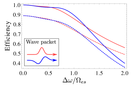
Figure 3: Dependence of the state transfer efficiency $\mid s\rangle\rightarrow\mid f\rangle$ on the bandwidth $\Delta\omega$ of the photonic wave packet for the fiber and cavity scenario (in units of $g_{es}$): The red (or lighter gray) lines are results of the Gaussian envelope $f_{\text{in}}^{1}(t)$ and the blue (or darker gray) lines of the antisymmetric envelope $f_{\text{in}}^{2}(t)$ . The parameters are: $g_{es}=g_{ef}=\kappa_{es}=\kappa_{ef}$ and $\gamma_{es},\gamma_{ef}\rightarrow 0$ (solid lines; i.e. conditions for high transfer efficiencies in (10) are fulfilled), $g_{es}=g_{ef}/\sqrt{2}=\kappa_{es}=\kappa_{ef}$ and $\gamma_{es},\gamma_{ef}\rightarrow 0$ (dashed lines; $2\chi_{es}=\chi_{ef}$ first condition in (10) is violated).

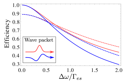
Figure 4: Dependence of the state transfer efficiency $\mid s\rangle\rightarrow\mid f\rangle$ on the bandwidth $\Delta\omega$ of the photonic wave packet for the waveguide scenario (in units of $\Gamma_{es}$): The red (or lighter gray) lines are results of a Gaussian envelope $f_{\text{in}}^{1}(t)$ and the blue (or darker gray) lines of an antisymmetric envelope $f_{\text{in}}^{2}(t)$ . The parameters are $\Gamma_{es}=\Gamma_{ef}$ and $\gamma_{es}=\gamma_{ef}=0$ (solid lines; i.e. conditions for high transfer efficiencies in (25) are fulfilled), $2\Gamma_{es}=\Gamma_{ef}$ and $\gamma_{es}=\gamma_{ef}=0$ (dashed lines; $2\chi_{es}=\chi_{ef}$ first condition in (25) is violated)

The solid lines in Fig. 3 and Fig. 4 correspond to the ideal scenario with high transfer efficiencies as described by Eqs. (10) for the fiber and cavity based scenario and by Eq. (25) for the waveguide scenario. As long as the bandwidth of the incoming photon wave packet is sufficiently small (see Eqs. (7) and (17)) the efficiency of the excitation transfer is close to unity and independent of the shape of the photon wave packet. The dashed lines in Fig. 3 and Fig. 4 describe cases with $2\chi_{es}=\chi_{ef}$ so that a violation of the first condition in Eq. (10) or in Eq. (25) limits the efficiency. If this impedance matching condition is violated the efficiency for triggering a state transfer is always below unity even in the limit of infinitely small bandwidth photons.

V Applications

Our scheme can serve as a basic building block for various tasks of quantum information processing. In this section, we discuss possible applications of our scheme for building a single atom single photon quantum memory and for implementing a deterministic frequency converter of photonic qubits.

V.1 Single atom single photon quantum memory

A photonic qubit stored in a polarization degree of freedom of a photon wave packet, for example, can be converted to a matter qubit and stored in the atomic level structure of the atom (for the reverse process see Cirac1997 ; Ritter ; trautmann2015time ). This can be achieved by using an atom with a level structure depicted in Fig. 5 (a), for example, with the atom initially prepared in state $\mid s\rangle$ and with the qubits states $\mid 0\rangle$ and $\mid 1\rangle$ constituting long lived stable states. If the properties of the photon emitted during this storage process are independent of the state of the initial photonic qubit no information about this photonic input state is transferred to the background or to the fiber modes involved. Thus, the photonic excitation transfer to the material degrees of freedom does not suffer from decoherence. For a cavity this condition can be fulfilled by choosing equal vacuum Rabi frequencies and cavity loss rates for the $\sigma^{\pm}$ transitions, i.e. $g_{\sigma^{-}}=g_{\sigma^{+}}$ and $\kappa_{\sigma^{-}}=\kappa_{\sigma^{+}}$. In the absence of a cavity for this purpose one has to choose equal photon emission rates into the waveguide, i.e. $\Gamma_{\sigma^{-}}=\Gamma_{\sigma^{+}}$. Hence, the scheme can be used to implement a heralded quantum memory with a fidelity close to unity. A deterministic quantum memory with near-unit fidelity can be implemented if the impedance matching conditions are fulfilled and $C_{\sigma_{\pm}}\gg 1$ in case of cavity or $\gamma_{\sigma^{\pm}}\ll\Gamma_{\sigma^{\pm}}$ in the absence of a cavity. Hereby, a coupling of the cavity modes to the $\Pi$ polarized transitions is not required, as these transitions can also be induced by spontaneous decay processes.

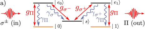
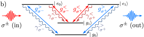
Figure 5: An atomic level structure for converting a polarization encoded photonic qubit encoded into a matter qubit (a) and for converting the frequency of a polarization encoded photonic qubit (b).

A possible level scheme, for the free space scenario can again be found in ${}^{40}\text{Ca}$, for example. The states $\mid 3p^{6}3d4s\;^{3}D\;J=1\;m_{J}=\pm 1\rangle$ could be used to encode the qubit, the states $\mid 3p^{6}3d4p\;^{3}D\;J=1\;m_{J}=\pm 1\rangle$ could serve as intermediate excited states and the state $\mid 3p^{6}3d4s\;^{3}D\;J=1\;m_{J}=0\rangle$ could serve as initial state. In this level scheme all the branching ratios are equal. The limiting factor is the decay to the manifold $3p^{6}3d4s\;^{3}D\;J=2$. The decay rate of the states in the manifold $3p^{6}3d4p\;^{3}D\;J=1$ to the manifold $3p^{6}3d4s\;^{3}D\;J=2$ is suppressed by a factor of $3$, as compared to the decay rate to the manifold $3p^{6}3d4s\;^{3}D\;J=1$ kostlin1964beitrag . However, more favorable level schemes might be found in other atoms, isotopes or artificial atoms. In the waveguide scenario or the cavity scenario the impedance matching condition stated in Eqs. (10) and (25) can not be connected directly to the dipole matrix elements of the optical transitions, as the modification of the mode structure due to the presence of the waveguide or the cavity (vacuum Rabi frequencies and leakage parameters) are also of relevance. However, this also allows for a greater tunability of the systems parameters. Hence, in a cavity or a waveguide it might be easier to fulfill the impedance matching condition than in the free space scenario.

V.2 Frequency converter

Our scheme can also be used for a deterministic frequency converter of photonic qubits. A possible atomic level structure performing frequency conversion of a polarization encoded photonic qubit is depicted in Fig. 5 (b). For converting the frequency of the photon the atom has to be prepared either in state $\mid g_{0}\rangle$ or in state $\mid g_{1}\rangle$ depending on whether the frequencies of the photon should be decreased or increased. For ensuring the emission of the resulting photon into a waveguide the corresponding vacuum Rabi frequencies or emission rates into the waveguide have to be sufficiently large. Hence, for a cavity it is required that $\gamma_{\sigma^{\pm}}^{>}\ll 2\mid g_{\sigma^{\pm}}^{>}\mid^{2}/\kappa_{\sigma^{\pm}}^{>}$ and $\gamma_{\sigma^{\pm}}^{<}\ll 2\mid g_{\sigma^{\pm}}^{<}\mid^{2}/\kappa_{\sigma^{\pm}}^{<}$. In the absence of a cavity, the conditions read $\gamma_{\sigma^{\pm}}^{>}\ll\Gamma_{\sigma^{\pm}}^{>}$ and $\gamma_{\sigma^{\pm}}^{<}\ll\Gamma_{\sigma^{\pm}}^{<}$. In addition to performing a frequency conversion, the fact that only a single atom is involved allows us to perform a nondestructive detection of the photon, by reading out the state of the atom.

VI Conclusions

In conclusion, we have proposed a dissipation dominated scheme for triggering highly efficient excitation transfer from a single photon wave packet of arbitrary shape but small bandwidth to a single quantum emitter. We have shown that by balancing the decay rates characterizing relevant dissipation processes, such as spontaneous photon emission into waveguides or the electromagnetic background, appropriately these processes can be turned into a valuable tool for purposes of quantum information processing. Our scheme offers the advantage that no additional control of the system by additional laser fields or by postselection is required. Thus, the scheme presented in this article paves the way to scalable quantum communication networks as it relaxes the restrictive requirements on the synchronization of the nodes of the network (detailed knowledge on the arrival time and shape of the photons is not required) and as it is not limited by the efficiency of single photon detectors. We have demonstrated that our scheme can be applied to a variety of different scenarios including fiber and cavity based architectures as well as architectures without any optical resonators. It can serve as a basic building block for various protocols relevant for quantum information processing. As examples we have discussed setups for a deterministic single atom single photon quantum memory and a deterministic frequency converter between photonic qubits of different wave lengths which could serve as an interface between several quantum information processing architectures.

Appendix A Derivation for Waveguide

In this appendix, we give a detailed derivation of Eq. (14), which describes the dynamics of the quantum emitter for the waveguide scenario. The derivation of Eq. (2) for the fiber and cavity scenario follows along the same lines. We start our considerations with the Ansatz for the time evolution of the wave function of Eq. (13) The Schrödinger equation induced by the Hamiltonian $\hat{H}_{\text{int}}^{\text{wg}}(t)$ is equivalent to the following set of differential equations

$$\frac{d}{dt}\psi_{e}(t) = \frac{i}{\hbar}\sum_{k\in\{es,ef\}}e^{i\omega_{k}\left(t-t_{0}\right)}\langle 0|^{\text{F}_{k}}\langle 0|^{\text{B}_{k}}\mathbf{d}_{k}^{*}\cdot\left(\mathbf{\hat{E}}_{\text{F}_{k}}^{+}(\mathbf{x}_{A},t)+\mathbf{\hat{E}}_{\text{B}_{k}}^{+}(\mathbf{x}_{A},t)\right)\mid\psi_{k}(t)\rangle^{\text{F}_{k},\text{B}_{k}}\;,$$ (28)

$$\mid\psi_{k}(t)\rangle^{\text{F}_{k},\text{B}_{k}} = \frac{i}{\hbar}e^{-i\omega_{k}\left(t-t_{0}\right)}\mathbf{d}_{k}\cdot\left(\mathbf{\hat{E}}_{\text{F}_{k}}^{-}(\mathbf{x}_{A},t)+\mathbf{\hat{E}}_{\text{B}_{k}}^{-}(\mathbf{x}_{A},t)\right)|0\rangle^{\text{F}_{k}}|0\rangle^{\text{B}_{k}}\psi_{e}(t)\;\text{for }k\in\left\{es,ef\right\}\;.$$ (29)

A general solution of the second equation is of the form

$$\mid\psi_{k}(t)\rangle^{\text{F}_{k},\text{B}_{k}} = \frac{i}{\hbar}\int_{t_{0}}^{t}e^{-i\omega_{k}\left(t^{\prime}-t_{0}\right)}\mathbf{d}_{k}\cdot\left(\mathbf{\hat{E}}_{\text{F}_{k}}^{-}(\mathbf{x}_{A},t^{\prime})+\mathbf{\hat{E}}_{\text{B}_{k}}^{-}(\mathbf{x}_{A},t^{\prime})\right)|0\rangle^{\text{F}_{k}}|0\rangle^{\text{B}_{k}}\psi_{e}(t^{\prime})dt^{\prime}$$

$$+\mid\psi_{k}(t_{0})\rangle^{\text{F}_{k},\text{B}_{k}}\;\text{for }k\in\left\{es,ef\right\}\;.$$

Inserting this expression into Eq. (28) and using the initial condition, i.e.

$$\mid\psi_{es}(t_{0})\rangle^{\text{F}_{ef},\text{B}_{ef}}=\mid\psi_{\text{in}}\rangle^{\text{F}_{es}}\mid 0\rangle^{\text{B}_{ef}}\text{ and }\mid\psi_{ef}(t_{0})\rangle^{\text{F}_{ef},\text{B}_{ef}}=\mid 0\rangle^{\text{F}_{ef}}\mid 0\rangle^{\text{B}_{ef}},$$

we obtain the equivalent integro differential equation

$$\frac{d}{dt}\psi_{e}(t) = -\frac{1}{\hbar^{2}}\sum_{k\in\{es,ef\}}\int_{t_{0}}^{t}e^{i\omega_{k}\left(t-t^{\prime}\right)}\langle 0|^{\text{F}_{k}}\langle 0|^{\text{B}_{k}}\left[\mathbf{d}_{k}^{*}\cdot\left(\mathbf{\hat{E}}_{\text{F}_{k}}^{+}(\mathbf{x}_{A},t)+\mathbf{\hat{E}}_{\text{B}_{k}}^{+}(\mathbf{x}_{A},t)\right)\right]$$

$$\left[\mathbf{d}_{k}\cdot\left(\mathbf{\hat{E}}_{\text{F}_{k}}^{-}(\mathbf{x}_{A},t^{\prime})+\mathbf{\hat{E}}_{\text{B}_{k}}^{-}(\mathbf{x}_{A},t^{\prime})\right)\right]|0\rangle^{\text{F}_{k}}|0\rangle^{\text{B}_{k}}\psi_{e}(t^{\prime})dt^{\prime}$$

$$+\frac{i}{\hbar}e^{i\omega_{es}\left(t-t_{0}\right)}\langle 0|^{\text{F}_{es}}\mathbf{d}_{k}^{*}\cdot\mathbf{\hat{E}}_{\text{F}_{es}}^{+}(\mathbf{x}_{A},t)\mid\psi_{\text{in}}\rangle^{\text{F}_{es}}.$$

Within the framework of the above mentioned approximations this expression yields a complete description of the one photon excitation process of the three level system. In particular, it also describes all possible non Markovian effects. However, it is well known that in the optical regime with spontaneous decay rates much smaller than atomic transition frequencies and for setups in which a photon emitted by an atom does not return to the atom at a later time, such as in free space or in an open waveguide, these non Markovian effects are negligible (see e.g. mollow1975pure for an early free space treatment). Hence, in the absence of such photon recurrence phenomena the above expression simplifies significantly and we obtain

$$\frac{d}{dt}\psi_{e}(t) = -\frac{1}{2}\left(\Gamma_{es}+\Gamma_{ef}+\gamma_{es}+\gamma_{ef}\right)\psi_{e}(t)$$ (30)

$$+i\sqrt{\Gamma_{es}}f_{in}(t)$$

with

$$\sqrt{\Gamma_{es}}f_{in}(t)=\frac{1}{\hbar}e^{i\omega_{es}\left(t-t_{0}\right)}\langle 0\mid\mathbf{d}_{es}^{*}\cdot\left(\mathbf{E}_{es}^{-}\right(\mathbf{x}_{A},t))^{\dagger}\mid\psi_{\text{in}}\rangle^{\text{F}_{es}}$$ (31)

describing the influence of the incoming single photon wave packet. The spontaneous decay rates induced by the reservoir modes $\text{F}_{es}$, $\text{F}_{ef}$, $\text{B}_{es}$, and $\text{B}_{ef}$ are denoted by $\Gamma_{es}$, $\Gamma_{ef}$, $\gamma_{es}$ and $\gamma_{ef}$ . Note that the basic structure of Eq. (30), especially the inhomogeneous term defined in Eq. (31), closely resembles Eq. (2) describing the dynamics in the cavity scenario. In fact, the derivation of both equations follows the same reasoning.

References

- (1) H. J. Kimble, The quantum internet, Nature 453, 1023 (2008).
- (2) M. Nielsen and I. L. Chuang, Quantum Computation and Quantum Information (Cambridge, Univ.Press, 2000).
- (3) B. Hensen et al., Loophole-free bell inequality violation using electron spins separated by 1.3 kilometres, Nature 526, 682 (2015).
- (4) M. Fleischhauer and M. D. Lukin, Dark-state polaritons in electromagnetically induced transparency, Phys. Rev. Lett. 84, 5094 (2000).
- (5) D. F. Phillips, A. Fleischhauer, A. Mair, R. L. Walsworth and M. D. Lukin, Storage of light in atomic vapor, Phys. Rev. Lett. 86, 783 (2001).
- (6) H. De Riedmatten, M. Afzelius, M. U. Staudt, C. Simon and N. Gisin, A solid-state light–matter interface at the single-photon level, Nature 456, 773 (2008).
- (7) J. I. Cirac, P. Zoller, H. J. Kimble and H. Mabuchi, Quantum state transfer and entanglement distribution among distant nodes in a quantum network, Phys. Rev. Lett. 78, 3221 (1997).
- (8) S. Ritter et al., An elementary quantum network of single atoms in optical cavities, Nature 484, 195 (2012).
- (9) L.-M. Duan and H. J. Kimble, Scalable photonic quantum computation through cavity-assisted interactions, Phys. Rev. Lett. 92, 127902 (2004).
- (10) A. Reiserer, S. Ritter and G. Rempe, Nondestructive detection of an optical photon, Science 342, 1349 (2013).
- (11) A. Reiserer, N. Kalb, G. Rempe and S. Ritter, A quantum gate between a flying optical photon and a single trapped atom, Nature 508, 237 (2014).
- (12) N. Kalb, A. Reiserer, S. Ritter and G. Rempe, Heralded storage of a photonic quantum bit in a single atom, Phys. Rev. Lett. 114, 220501 (2015).
- (13) W. Happer, Optical pumping, Revi. Mod. Phys. 44, 169 (1972).
- (14) A. Akimov et al., Generation of single optical plasmons in metallic nanowires coupled to quantum dots, Nature 450, 402 (2007).
- (15) J. A. Schuller et al., Plasmonics for extreme light concentration and manipulation, Nat. Mater. 9, 193 (2010).
- (16) E. Vetsch et al., Optical interface created by laser-cooled atoms trapped in the evanescent field surrounding an optical nanofiber, Phys. Rev. Lett. 104, 203603 (2010).
- (17) J. You and F. Nori, Atomic physics and quantum optics using superconducting circuits, Nature 474, 589 (2011).
- (18) R. Maiwald et al., Collecting more than half the fluorescence photons from a single ion, Phys. Rev. A 86, 043431 (2012).
- (19) M. Fischer et al., Efficient saturation of an ion in free space, Applied Physics B 117, 797 (2014).
- (20) U. Fano, Sullo spettro di assorbimento dei gas nobili presso il limite dello spettro d′arco, Il Nuovo Cimento 12, 154 (1935).
- (21) U. Fano, Effects of configuration interaction on intensities and phase shifts, Phys. Rev. 124, 1866 (1961).
- (22) P. W. Anderson, Localized magnetic states in metals, Phys. Rev. 124, 41 (1961).
- (23) C. Gardiner and P. ZollerQuantum noise Vol. 56 (Springer Science & Business Media, 2004).
- (24) B. Mollow, Pure-state analysis of resonant light scattering: Radiative damping, saturation, and multiphoton effects, Phys. Rev. A 12, 1919 (1975).
- (25) The dynamical model of Eq.(2) is a a Fano-Anderson-type model fano1935sullo ; fano1961effects ; anderson1961localized treated in the pole approximation.
- (26) A. Kuhn, M. Hennrich and G. Rempe, Deterministic single-photon source for distributed quantum networking, Phys. Rev. Lett. 89, 067901 (2002).
- (27) C. M. Bender and S. A. Orszag, Advanced Mathematical Methods for Scientists and Engineers I (Springer Science & Business Media, 1999).
- (28) J. Petersen, J. Volz and A. Rauschenbeutel, Chiral nanophotonic waveguide interface based on spin-orbit interaction of light, Science 346, 67 (2014).
- (29) J. Lin et al., Polarization-controlled tunable directional coupling of surface plasmon polaritons, Science 340, 331 (2013).
- (30) R. Mitsch, C. Sayrin, B. Albrecht, P. Schneeweiss and A. Rauschenbeutel, Quantum state-controlled directional spontaneous emission of photons into a nanophotonic waveguide, Nat. Commun. 5, 5713 (2014).
- (31) A. Goban et al., Atom–light interactions in photonic crystals, Nat. Commun. 5, 3808 (2014).
- (32) M. Stobińska, G. Alber and G. Leuchs, Perfect excitation of a matter qubit by a single photon in free space, Europhys. Lett. 86, 14007 (2009).
- (33) H. Köstlin, Ein Beitrag zur experimentellen Bestimmung von Übergangswahrscheinlichkeiten in der Atomhülle und deren Messung im Spektrum von Kalzium, Zeitschrift für Physik 178, 200 (1964).
- (34) I. Marzoli, J. I. Cirac, R. Blatt and P. Zoller, Laser cooling of trapped three-level ions: Designing two-level systems for sideband cooling, Phys. Rev. A 49, 2771 (1994).
- (35) N. Trautmann, G. Alber, G. S. Agarwal and G. Leuchs, Time-reversal-symmetric single-photon wave packets for free-space quantum communication, Phys. Rev. Lett. 114, 173601 (2015).