Adjusting for Chance Clustering Comparison Measures

Abstract

Adjusted for chance measures are widely used to compare partitions/clusterings of the same data set. In particular, the Adjusted Rand Index (ARI) based on pair-counting, and the Adjusted Mutual Information (AMI) based on Shannon information theory are very popular in the clustering community. Nonetheless it is an open problem as to what are the best application scenarios for each measure and guidelines in the literature for their usage are sparse, with the result that users often resort to using both. Generalized Information Theoretic (IT) measures based on the Tsallis entropy have been shown to link pair-counting and Shannon IT measures. In this paper, we aim to bridge the gap between adjustment of measures based on pair-counting and measures based on information theory. We solve the key technical challenge of analytically computing the expected value and variance of generalized IT measures. This allows us to propose adjustments of generalized IT measures, which reduce to well known adjusted clustering comparison measures as special cases. Using the theory of generalized IT measures, we are able to propose the following guidelines for using ARI and AMI as external validation indices: ARI should be used when the reference clustering has large equal sized clusters; AMI should be used when the reference clustering is unbalanced and there exist small clusters.

Keywords: Clustering Comparisons, Adjustment for Chance, Generalized Information Theoretic Measures

1 Introduction

Clustering comparison measures are used to compare partitions/clusterings of the same data set. In the clustering community (Aggarwal and Reddy, 2013), they are extensively used for external validation when the ground truth clustering is available. A family of popular clustering comparison measures are measures based on pair-counting (Albatineh et al., 2006). This category comprises the well known similarity measures Rand Index (RI) (Rand, 1971) and the Jaccard coefficient (J) (Ben-Hur et al., 2001). Recently, information theoretic (IT) measures have been also extensively used to compare partitions (Strehl and Ghosh, 2003; Vinh et al., 2010). Given the variety of different possible measures, it is very challenging to identify the best choice for a particular application scenario (Wu et al., 2009).

The picture becomes even more complex if adjusted for chance measures are also considered. Adjusted for chance measures are widely used external clustering validation techniques because they improve the interpretability of the results. Indeed, two important properties hold true for adjusted measures: they have constant baseline equal to 0 value when the partitions are random and independent, and they are equal to 1 when the compared partitions are identical. Notable examples are the Adjusted Rand Index (ARI) (Hubert and Arabie, 1985) and the Adjusted Mutual Information (AMI) (Vinh et al., 2009). It is common to see published research that validates clustering solutions against a reference ground truth clustering with the ARI or the AMI. Nonetheless there are still open problems: there are no guidelines for their best application scenarios shown in the literature to date and authors often resort to employing them both and leaving the reader to interpret.

Moreover, some clustering comparisons measures are susceptible to selection bias: when selecting the most similar partition to a given ground truth partition, clustering comparison measures are more likely to select partitions with many clusters (Romano et al., 2014). In Romano et al. (2014) it was shown that it is beneficial to perform statistical standardization to IT measures to correct for this bias. In particular, standardized IT measures help in decreasing this bias when the number of objects in the data set is small. Statistical standardization has not been applied to pair-counting measures yet in the literature. We solve this challenge in the current paper, and provide further results about the utility of measure adjustment by standardization.

In this work, we aim to bridge the gap between the adjustment of pair-counting measures and the adjustment of IT measures. In Furuichi (2006); Simovici (2007) it has been shown that generalized IT measures based on the Tsallis $q$-entropy (Tsallis et al., 2009) are a further generalization of IT measures and some pair-counting measures such as RI. In this paper, we will exploit this useful idea to connect ARI and AMI. Furthermore using the same idea, we can perform statistical adjustment by standardization to a broader class of measures, including pair-counting measures.

A key technical challenge is to analytically compute the expected value and variance for generalized IT measures when the clusterings are random. To solve this problem, we propose a technique applicable to a broader class of measures we name $\mathcal{L}_{\phi}$, which includes generalized IT measures as a special case. This generalizes previous work which provided analytical adjustments for narrower classes: measures based on pair-counting from the family $\mathcal{L}$ (Albatineh et al., 2006), and measures based on the Shannon’s mutual information (Vinh et al., 2009, 2010). Moreover, we define a family of measures $\mathcal{N}_{\phi}$ which generalizes many clustering comparison measures. For measures belonging to this family, the expected value can be analytically approximated when the number of objects is large. Table 1 summarizes the development of this line of work over the past 30 years and positions our contribution.

In summary, we make the following contributions:

• We define families of measures for which the expected value and variance can be computed analytically when the clusterings are random;

• We propose generalized adjusted measures to correct for the baseline property and for selection bias. This captures existing well known measures as special cases;

• We provide insights into the open problem of identifying the best application scenarios for clustering comparison measures, in particular the application scenarios for ARI and AMI.

Figure 1: Families of clustering comparison measures.

Year	Contribution	Reference
1985	Expectation of Rand Index (RI)	(Hubert and Arabie, 1985)
2006	Expectation and variance of $S\in\mathcal{L}$	(Albatineh et al., 2006)
2009	Expectation of Shannon Mutual Information (MI)	(Vinh et al., 2009)
2010	Expectation of Normalized Shannon MI (NMI)	(Vinh et al., 2010)
2014	Variance of Shannon MI	(Romano et al., 2014)
2015	Expectation and variance of $S\in\mathcal{L}_{\phi}$ Asymptotic expectation of $S\in\mathcal{N}_{\phi}$	This Work

Table 1: Survey of analytical computation of measures.

2 Comparing Partitions

Given two partitions (clusterings) $U$ and $V$ of the same data set of $N$ objects, let $\{u_{1},\dots,u_{r}\}$ and $\{v_{1},\dots,v_{c}\}$ be the disjoint sets (clusters) for $U$ and $V$ respectively. Let $|u_{i}|=a_{i}$ for $i=1,\dots,r$ denote the number of objects in the set $u_{i}$ and $|v_{j}|=b_{j}$ for $j=1,\dots,c$ denote the number of objects in $v_{j}$. Naturally, $\sum_{i=1}^{r}a_{i}=\sum_{j=1}^{c}b_{j}=N$. The overlap between the two partitions $U$ and $V$ can be represented in matrix form by a $r\times c$ contingency table $\mathcal{M}$ where $n_{ij}$ represents the number of objects in both $u_{i}$ and $v_{j}$, i.e. $n_{ij}=|u_{i}\cap v_{j}|$. Also, we refer to $a_{i}=\sum_{i=1}^{r}n_{ij}$ as the row marginals and to $b_{j}=\sum_{j=1}^{c}n_{ij}$ as the column marginals. A contingency table $\mathcal{M}$ is shown in Table 2.

		$V$
		$b_{1}$	$\cdots$	$b_{j}$	$\cdots$	$b_{c}$
	$a_{1}$	$n_{11}$	$\cdots$	$\cdot$	$\cdots$	$n_{1c}$
	$\vdots$	$\vdots$		$\vdots$		$\vdots$
$U$	$a_{i}$	$\cdot$		$n_{ij}$		$\cdot$
	$\vdots$	$\vdots$		$\vdots$		$\vdots$
	$a_{r}$	$n_{r1}$	$\cdots$	$\cdot$	$\cdots$	$n_{rc}$

Table 2: $r\times c$ contingency table $\mathcal{M}$ related to two clusterings $U$ and $V$. $a_{i}=\sum_{j}n_{ij}$ are the row marginals and $b_{j}=\sum_{i}n_{ij}$ are the column marginals.

Pair-counting measures between partitions, such as the Rand Index (RI) (Rand, 1971), might be defined using the following quantities: $k_{11}$, the pairs of objects in the same set in both $U$ and $V$; $k_{00}$ the pairs of objects not in the same set in $U$ and not in the same set in $V$; $k_{10}$, the pairs of objects in the same set in $U$ and not in the same set in $V$; and $k_{01}$ the pairs of objects not in the same set in $U$ and in the same set in $V$. All these quantities can be computed using the contingency table $\mathcal{M}$, for example:

$$k_{11}=\frac{1}{2}\sum_{i=1}^{r}\sum_{j=1}^{c}n_{ij}(n_{ij}-1),\quad k_{00}=\frac{1}{2}\Big{(}N^{2}+\sum_{i=1}^{r}\sum_{j=1}^{c}n_{ij}^{2}-\Big{(}\sum_{i=1}^{r}a_{i}^{2}+\sum_{j=1}^{c}b_{j}^{2}\Big{)}\Big{)}$$ (1)

Using $k_{00}$, $k_{11}$, $k_{10}$, and $k_{01}$ it is possible to compute similarity measures, e.g. RI, or distance measures, e.g. the Mirkin index $\mbox{MK}(U,V)\triangleq\sum_{i}a_{i}^{2}+\sum_{j}b_{j}^{2}-2\sum_{i,j}n_{ij}^{2}$, between partitions (Meilă, 2007):

$$\mbox{RI}(U,V)\triangleq(k_{11}+k_{00})/\binom{N}{2},\quad\mbox{MK}(U,V)=2(k_{10}+k_{01})=N(N-1)(1-\mbox{RI}(U,V))$$ (2)

Information theoretic measures are instead defined for random variables but can also be used to compare partitions when the we employ the empirical probability distributions associated to $U$, $V$, and the joint partition $(U,V)$. Let $\frac{a_{i}}{N}$, $\frac{b_{j}}{N}$, and $\frac{n_{ij}}{N}$ be the probability that an object falls in the set $u_{i}$, $v_{j}$, and $u_{i}\cap v_{j}$ respectively. We can therefore define the Shannon entropy with natural logarithms for a partition $V$ as follows: $H(V)\triangleq-\sum_{j}\frac{b_{j}}{N}\ln{\frac{b_{j}}{N}}$. Similarly, we can define the entropy $H(U)$ for the partition $U$, the joint entropy $H(U,V)$ for the joint partition $(U,V)$, and the conditional entropies $H(U|V)$ and $H(V|U)$. Shannon entropy can be used to define the well know mutual information (MI) and employ it to compute similarity between partitions $U$ and $V$:

$$\mbox{MI}(U,V)\triangleq H(U)-H(U|V)=H(V)-H(V|U)=H(U)+H(V)-H(U,V)$$ (3)

On contingency tables, MI is linearly related to $G$-statistics used for likelihood-ratio tests: $G=2N\mbox{MI}$. In Meilă (2007), using the Shannon entropy it was shown that the following distance, namely the variation of information (VI) is a metric:

$$\mbox{VI}(U,V)\triangleq 2H(U,V)-H(U)-H(V)=H(U|V)+H(V|U)=H(U)+H(V)-2\mbox{MI}(U,V)$$ (4)

2.1 Generalized Information Theoretic Measures

Generalized Information Theoretic (IT) measures based on the generalized Tsallis $q$-entropy (Tsallis, 1988) can be defined for random variables (Furuichi, 2006) and also be applied to the task of comparing partitions (Simovici, 2007). Indeed, these measures have also seen recent application in the machine learning community. More specifically, it has been shown that they can act as proper kernels (Martins et al., 2009). Furthermore, empirical studies demonstrated that careful choice of $q$ yields successful results when comparing the similarity between documents (Vila et al., 2011), decision tree induction (Maszczyk and Duch, 2008), and reverse engineering of biological networks (Lopes et al., 2011). It is important to note that the Tsallis $q$-entropy is equivalent to the Harvda-Charvat-Daróczy generalized entropy proposed in Havrda and Charvát (1967); Daróczy (1970). Results available in literature about these generalized entropies are equivalently valid for all the proposed versions.

Given $q\in\mathbb{R}^{+}-\{1\}$, the generalized Tsallis $q$-entropy for a partition $V$ is defined as follows: $H_{q}(V)\triangleq\frac{1}{q-1}\big{(}1-\sum_{i}\big{(}\frac{b_{j}}{N}\big{)}^{q}\big{)}$. Similarly to the case of Shannon entropy, we have the joint $q$-entropy $H_{q}(U,V)$ and the conditional $q$-entropies $H_{q}(U|V)$ and $H_{q}(V|U)$. Conditional $q$-entropy is computed according to a weighted average parametrized in $q$. More specifically the formula for $H_{q}(V|U)$ is:

$$H_{q}(V|U)\triangleq\sum_{i=1}^{r}\Big{(}\frac{a_{i}}{N}\Big{)}^{q}H_{q}(V|u_{i})=\sum_{i=1}^{r}\Big{(}\frac{a_{i}}{N}\Big{)}^{q}\frac{1}{q-1}\Big{(}1-\sum_{j=1}^{c}\Big{(}\frac{n_{ij}}{a_{i}}\Big{)}^{q}\Big{)}$$ (5)

The $q$-entropy reduces to the Shannon entropy computed in nats for $q\rightarrow 1$.

In Furuichi (2006), using the fact that $q>1$ implies $H_{q}(U)\geq H_{q}(U|V)$, it is shown that non-negative MI can be naturally generalized with $q$-entropy when $q>1$:

$$\mbox{MI}_{q}(U,V)\triangleq H_{q}(U)-H_{q}(U|V)=H_{q}(V)-H_{q}(V|U)=H_{q}(U)+H_{q}(V)-H_{q}(U,V)$$ (6)

However, $q$ values smaller than 1 are allowed if the assumption that MI${}_{q}(U,V)$ is always positive can be dropped. In addition, generalized entropic measures can be used to defined the generalized variation of information distance ($\mbox{VI}_{q}$) which tends to VI in Eq. (4) when $q\rightarrow 1$:

$$\mbox{VI}_{q}(U,V)\triangleq H_{q}(U|V)+H_{q}(V|U)=2H_{q}(U,V)-H_{q}(U)-H_{q}(V)=H_{q}(U)+H_{q}(V)-2\mbox{MI}_{q}(U,V)$$ (7)

In Simovici (2007) it was shown that $\mbox{VI}_{q}$ is a proper metric and interesting links were identified between measures for comparing partitions $U$ and $V$. We state these links in Proposition 1 given that they set the fundamental motivation of our paper:

Proposition 1

(Simovici, 2007) When $q=2$ the generalized variation of information, the Mirkin index, and the Rand index are linearly related: $\mbox{\emph{VI}}_{2}(U,V)=\frac{1}{N^{2}}\mbox{\emph{MK}}(U,V)=\frac{N-1}{N}(1-\mbox{\emph{RI}}(U,V))$.

Generalized IT measures are not only a generalization of IT measures in the Shannon sense but also a generalization of pair-counting measures for particular values of $q$.

2.2 Normalized Generalized IT Measures

To allow a more interpretable range of variation, a clustering similarity measure should be normalized: it should achieve its maximum at 1 when $U=V$. An upper bound to the generalized mutual information MI_q is used to obtained a normalized measure. $\mbox{MI}_{q}$ can take different possible upper bounds (Furuichi, 2006). Here, we choose to derive another possible upper bound using Eq. (7) when we use the minimum value of $\mbox{VI}_{q}=0$: $\max{\mbox{MI}_{q}}=\frac{1}{2}(H_{q}(U)+H_{q}(V))$. This upper bound is valid for any $q\in\mathbb{R}^{+}-\{1\}$ and allows us to link different existing measures as we will show in the next sections of the paper. The Normalized Mutual Information with $q$-entropy (NMI_q) is defined as follows:

$$\mbox{NMI}_{q}(U,V)\triangleq\frac{\textup{MI}_{q}(U,V)}{\max{\textup{MI}_{q}(U,V)}}=\frac{\textup{MI}_{q}(U,V)}{\frac{1}{2}\big{(}H_{q}(U)+H_{q}(V)\big{)}}=\frac{H_{q}(U)+H_{q}(V)-H_{q}(U,V)}{\frac{1}{2}\big{(}H_{q}(U)+H_{q}(V)\big{)}}$$ (8)

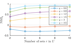
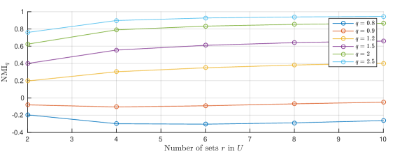
Even if NMI${}_{q}(U,V)$ achieves its maximum 1 when the partitions $U$ and $V$ are identical, NMI${}_{q}(U,V)$ is not a suitable clustering comparison measure. Indeed, it does not show constant baseline value equal to 0 when partitions are random. We explore this through an experiment. Given a dataset of $N=100$ objects, we randomly generate uniform partitions $U$ with $r=2,4,6,8,10$ sets and $V$ with $c=6$ sets independently from each others. The average value of $\mbox{NMI}_{q}$ over $1,000$ simulations for different values of $q$ is shown in Figure 2. It is reasonable to expect that when the partitions are independent, the average value of $\mbox{NMI}_{q}$ is constant irrespectively of the number of sets $r$ of the partition $U$. This is not the case. This behaviour is unintuitive and misleading when comparing partitions.

Figure 2: The baseline value of $\mbox{NMI}_{q}$ between independent partitions is not constant.

Computing the analytical expected value of generalized IT measures under the null hypothesis of random and independent $U$ and $V$ is important; it can be subtracted from the measure itself to adjust its baseline for chance such that their value is 0 when $U$ and $V$ are random. Given Proposition 1, this strategy also allows us to generalize adjusted for chance pair-counting and Shannon IT measures.

3 Baseline Adjustment

In order to adjust the baseline of a similarity measure $S(U,V)$, we have to compute its expected value under the null hypothesis of independent partitions $U$ and $V$. We adopt the assumption used for RI (Hubert and Arabie, 1985) and the Shannon MI (Vinh et al., 2009): partitions $U$ and $V$ are generated independently with fixed number of points $N$ and fixed marginals $a_{i}$ and $b_{j}$; this is also denoted as the permutation or the hypergeometric model of randomness. We are able to compute the exact expected value for a similarity measure in the family $\mathcal{L}_{\phi}$:

Definition 1

Let $\mathcal{L}_{\phi}$ be the family of similarity measures $S(U,V)=\alpha+\beta\sum_{ij}\phi_{ij}(n_{ij})$ where $\alpha$ and $\beta$ do not depend on the entries $n_{ij}$ of the contingency table $\mathcal{M}$ and $\phi_{ij}(\cdot)$ are bounded real functions.

Intuitively, $\mathcal{L}_{\phi}$ represents the class of measures that can be written as a linear combination of $\phi_{ij}(n_{ij})$. A measure between partitions uniquely determines $\alpha$, $\beta$, and $\phi_{ij}$. However, not every choice of $\alpha$, $\beta$, and $\phi_{ij}$ yields a meaningful similarity measure. $\mathcal{L}_{\phi}$ is a superset of the set of $\mathcal{L}$ defined in Albatineh et al. (2006) as the family of measures $S(U,V)=\alpha+\beta\sum_{ij}n_{ij}^{2}$, i.e. $S\in\mathcal{L}$ are special cases of measures in $\mathcal{L}_{\phi}$ with $\phi_{ij}(\cdot)=(\cdot)^{2}$. Figure 1 shows a diagram of the similarity measures discussed in Section 2.1 and their relationships.

Lemma 1

If $S(U,V)\in\mathcal{L}_{\phi}$, when partitions $U$ and $V$ are random:

$$E[S(U,V)]=\alpha+\beta\sum_{ij}E[\phi_{ij}(n_{ij})]\quad\text{ where }\quad E[\phi_{ij}(n_{ij})]\quad\text{ is }\$$ (9)

$$\sum_{n_{ij}=\max\{0,a_{i}+b_{j}-N\}}^{\min\{a_{i},b_{j}\}}\phi_{ij}(n_{ij})\frac{a_{i}!b_{j}!(N-a_{i})!(N-b_{j})!}{N!n_{ij}!(a_{i}-n_{ij})!(b_{j}-n_{ij})!(N-a_{i}-b_{j}+n_{ij})!}$$ (10)

Lemma 1 extends the results in Albatineh and Niewiadomska-Bugaj (2011) showing exact computation of the expected value of measures in the family $\mathcal{L}$. Given that generalized IT measures belong in $\mathcal{L}_{\phi}$ we can employ this result to adjust them.

3.1 Baseline Adjustment for Generalized IT measures

Using Lemma 1 it is possible to compute the exact expected value of $H_{q}(U,V)$, $\mbox{VI}_{q}(U,V)$ and $\mbox{MI}_{q}(U,V)$:

Theorem 1

When the partitions $U$ and $V$ are random:

1. $E[H_{q}(U,V)]=\frac{1}{q-1}\Big{(}1-\frac{1}{N^{q}}\sum_{ij}E[n_{ij}^{q}]\Big{)}$ with $E[n_{ij}^{q}]$ from Eq. (10) with $\phi_{ij}(n_{ij})=n_{ij}^{q}$;

2. $E[\mbox{\emph{MI}}_{q}(U,V)]=H_{q}(U)+H_{q}(V)-E[H_{q}(U,V)]$;

3. $E[\mbox{\emph{VI}}_{q}(U,V)]=2E[H_{q}(U,V)]-H_{q}(U)-H_{q}(V)$.

It is worth noting that this approach is valid for any $q\in\mathbb{R}^{+}-\{1\}$. We can use these expected values to adjust for baseline generalized IT measures. We use the method proposed in Hubert and Arabie (1985) to adjust similarity measures, such as $\mbox{MI}_{q}$, and distance measures, such as $\mbox{VI}_{q}$:

$$\mbox{AMI}_{q}\triangleq\frac{\mbox{MI}_{q}-E[\mbox{MI}_{q}]}{\max{\mbox{MI}_{q}}-E[\mbox{MI}_{q}]}\quad\mbox{AVI}_{q}\triangleq\frac{E[\mbox{VI}_{q}]-\mbox{VI}_{q}}{E[\mbox{VI}_{q}]-\min{\mbox{VI}_{q}}}$$ (11)

$\mbox{VI}_{q}$ is a distance measure, thus $\min{\mbox{VI}_{q}}=0$. For MI_q we use the upper bound $\max{\mbox{MI}_{q}}=\frac{1}{2}\big{(}H_{q}(U)+H_{q}(V)\big{)}$ as for NMI_q in Eq. (8). An exhaustive list of adjusted versions of Shannon MI can be found in Vinh et al. (2010), when the upper bound $\frac{1}{2}(H_{q}(U)+H_{q}(V))$ is used the authors named the adjusted MI as $\mbox{AMI}_{\textup{sum}}$.

It is important to note that this type of adjustment turns distance measures into similarity measures, i.e., $\mbox{AVI}_{q}$ is a similarity measure. It is also possible to maintain both the distance properties and the baseline adjustment using $\mbox{NVI}_{q}\triangleq\mbox{VI}_{q}/E[\mbox{VI}_{q}]$ which can be seen as a normalization of $\mbox{VI}_{q}$ with the stochastic upper bound $E[\mbox{VI}_{q}]$ (Vinh et al., 2009). It is also easy to see that $\mbox{AVI}_{q}=1-\mbox{NVI}_{q}$. The adjustments in Eq. (11) also enable the measures to be normalized. $\mbox{AMI}_{q}$ and $\mbox{AVI}_{q}$ achieve their maximum at 1 when $U=V$ and their minimum is 0 when $U$ and $V$ are random partitions.

According to the chosen upper bound for MI_q, we obtain the nice analytical form shown in Theorem 2. Our adjusted measures quantify the discrepancy between the values of the actual contingency table and their expected value in relation to the maximum discrepancy possible, i.e. the denominator in Eq. (12). It is also easy to see that all measures in $\mathcal{L}_{\phi}$ resemble this form when adjusted.

Theorem 2

Using $E[n_{ij}^{q}]$ in Eq. (10) with $\phi_{ij}(n_{ij})=n_{ij}^{q}$, the adjustments for chance for $\mbox{\emph{MI}}_{q}(U,V)$ and $\mbox{\emph{VI}}_{q}(U,V)$ are:

$$\mbox{\emph{AMI}}_{q}(U,V)=\mbox{\emph{AVI}}_{q}(U,V)=\frac{\sum_{ij}n_{ij}^{q}-\sum_{ij}E[n_{ij}^{q}]}{\frac{1}{2}\Big{(}\sum_{i}a_{i}^{q}+\sum_{j}b_{j}^{q}\Big{)}-\sum_{ij}E[n_{ij}^{q}]}$$ (12)

From now on we only discuss AMI_q, given that it is identical to AVI_q. There are notable special cases for our proposed adjusted generalized IT measures. In particular, the Adjusted Rand Index (ARI) (Hubert and Arabie, 1985) is just equal to AMI₂. ARI is a classic measure, heavily used for validation in social sciences and the most popular clustering validity index.

Corollary 1

It holds true that:
i) $\lim_{q\rightarrow 1}\mbox{\emph{AMI}}_{q}=\lim_{q\rightarrow 1}\mbox{\emph{AVI}}_{q}=\mbox{\emph{AMI}}=\mbox{\emph{AVI}}$ with Shannon entropy;
ii) $\mbox{\emph{AMI}}_{2}=\mbox{\emph{AVI}}_{2}=\mbox{\emph{ARI}}$.

Therefore, using the permutation model we can perform baseline adjustment to generalized IT measures. Our generalized adjusted IT measures are a further generalization of particular well known adjusted measures such as AMI and ARI. It is worth noting, that ARI is equivalent to other well known measures for comparing partitions (Albatineh et al., 2006). Furthermore, there is also a strong connection between ARI and Cohen’s $\kappa$ statistics used to quantify inter-rater agreement (Warrens, 2008).

Computational complexity:

The computational complexity of $\mbox{AMI}_{q}$ in Eq. (12) is dominated by the computation of the sum of the expected value of each cell.

Proposition 2

The computational complexity of $\mbox{\emph{AMI}}_{q}$ is $O(N\cdot\max{\{r,c\}})$.

If all the possible contingency tables $\mathcal{M}$ obtained by permutations were generated, the computational complexity of the exact expected value would be $O(N!)$. However, this can be dramatically reduced using properties of the expected value.

3.2 Experiments on Measure Baseline

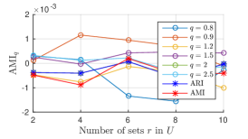
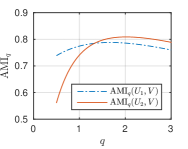
Here we show that our adjusted generalized IT measures have a baseline value of 0 when comparing random partitions $U$ and $V$. In Figure 3 we show the behaviour of $\mbox{AMI}_{q}$, ARI, and AMI on the same experiment proposed in Section 2.2. They are all close to 0 with negligible variation when the partitions are random and independent. Moreover, it is interesting to see the equivalence of $\mbox{AMI}_{2}$ and ARI. On the other hand, the equivalence of $\mbox{AMI}_{q}$ and AMI with Shannon’s entropy is obtained only at the limit $q\rightarrow 1$.

Figure 3: When varying the number of sets for the random partition $U$, the value of $\mbox{AMI}_{q}(U,V)$ is always very close to 0 with negligible variation for any $q$.

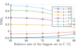
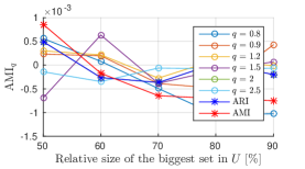
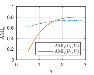
We also point out that $\mbox{NMI}_{q}$ does not show constant baseline when the relative size of the sets in $U$ varies when $U$ and $V$ are random. In Figure 4, we generate random partitions $V$ with $c=6$ sets on $N=100$ points, and random binary partitions $U$ independently. $\mbox{NMI}_{q}(U,V)$ shows different behavior at the variation of the relative size of the biggest set in $U$. This is unintuitive given that the partitions $U$ and $V$ are random and independent. We obtain the desired property of a baseline value of 0 with $\mbox{AMI}_{q}$.

Figure 4: When varying the relative size of one cluster for the random partition $U$, the value of $\mbox{AMI}_{q}(U,V)$ is always very close to 0 with negligible variation for any $q$.

3.3 Large Number of Objects

In this section, we introduce a very general family of measures which includes $\mathcal{L}_{\phi}$. For measures belonging to this family, it is possible to find an approximation of their expected value when the number of objects $N$ is large. This allows us to identify approximations for the expected value of measures in $\mathcal{L}_{\phi}$ as well as for measures not in $\mathcal{L}_{\phi}$, such as the Jaccard coefficient as shown in Figure 1.

Let $\mathcal{N}_{\phi}$ be the family of measures which are non-linear combinations of $\phi_{ij}(n_{ij})$:

Definition 2

Let $\mathcal{N}_{\phi}$ be the family of similarity measures $S(U,V)=\phi(\frac{n_{11}}{N},\dots,\frac{n_{ij}}{N},\dots,\frac{n_{rc}}{N})$ where $\phi$ is a bounded real function as $N$ reaches infinity.

Note that $\mathcal{N}_{\phi}$ is a generalization of $\mathcal{L}_{\phi}$. At the limit of large number of objects $N$, it is possible to compute the expected value of measures in $\mathcal{N}_{\phi}$ under random partitions $U$ and $V$ using only the marginals of the contingency table $\mathcal{M}$:

Lemma 2

If $S(U,V)\in\mathcal{N}_{\phi}$, then $\lim_{N\rightarrow+\infty}E[S(U,V)]=\phi\Big{(}\frac{a_{1}}{N}\frac{b_{1}}{N},\dots,\frac{a_{i}}{N}\frac{b_{j}}{N},\dots,\frac{a_{r}}{N}\frac{b_{c}}{N}\Big{)}$.

In Morey and Agresti (1984) the expected value of the RI was computed using an approximated value based on the multinomial distribution. It turns out this approximated value is equal to what we obtain for RI using Lemma 2. The authors of (Albatineh et al., 2006) noticed that the difference between the approximation and the expected value obtained with the hypergeometric model is small on empirical experiments when $N$ is large. We point out that this is a natural consequence of Lemma 2 given that $\mbox{RI}\in\mathcal{L}_{\phi}\subseteq\mathcal{N}_{\phi}$. Moreover, the multinomial distribution was also used to compute the expected value of the Jaccard coefficient (J) in Albatineh and Niewiadomska-Bugaj (2011), obtaining good results on empirical experiments with many objects. Again, this is a natural consequence of Lemma 2 given that $\mbox{J}\in\mathcal{N}_{\phi}$ but $\mbox{J}\notin\mathcal{L}_{\phi}$.

Generalized IT measures belong in $\mathcal{L}_{\phi}\subseteq\mathcal{N}_{\phi}$. Therefore we can employ Lemma 2. When the number of objects is large, the expected value under random partitions $U$ and $V$ of $H_{q}(U,V)$, MI${}_{q}(U,V)$, and VI${}_{q}(U,V)$ in Theorem 1 depends only on the entropy of the partitions $U$ and $V$:

Theorem 3

It holds true that:

1. $\lim_{N\rightarrow+\infty}E[H_{q}(U,V)]=H_{q}(U)+H_{q}(V)-(q-1)H_{q}(U)H_{q}(V)$;

2. $\lim_{N\rightarrow+\infty}E[\mbox{\emph{MI}}_{q}(U,V)]=(q-1)H_{q}(U)H_{q}(V)$;

3. $\lim_{N\rightarrow+\infty}E[\mbox{\emph{VI}}_{q}(U,V)]=H_{q}(U)+H_{q}(V)-2(q-1)H_{q}(U)H_{q}(V)$.

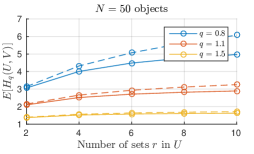
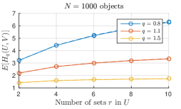
Result i) recalls the property of non-additivity that holds true for random variables (Furuichi, 2006). Figure 5 shows the behaviour of $E[H_{q}(U,V)]$ when the partitions $U$ and $V$ are generated uniformly at random. $V$ has $c=6$ sets and $U$ has $r$ sets. On this case, $H_{q}(U)+H_{q}(V)-(q-1)H_{q}(U)H_{q}(V)$ appears to be a good approximation already for $N=1000$. In particular, the approximation is good when the number of records $N$ is big with regards to the number of cells of the contingency table in Table 2: i.e., when $\frac{N}{r\cdot c}$ is large enough.

(a) Approximation on smaller sample size

(b) Approximation on bigger sample size

Figure 5: $E[H_{q}(U,V)]$ (solid) and their limit value $H_{q}(U)+H_{q}(V)-(q-1)H_{q}(U)H_{q}(V)$ (dashed). The solid line coincides approximately with the dashed one in 4(b) when $N=1000$. The limit value is a good approximation for $E[H_{q}(U,V)]$ when $\frac{N}{r\cdot c}$ is large enough.

4 Application scenarios for AMI_q

In this section we aim to answer to the question: Given a reference ground truth clustering $V$, which is the best choice for $q$ in AMI${}_{q}(U,V)$ to validate the clustering solution $U$? By answering this question, we implicitly identify the application scenarios for ARI and AMI given the results in Corollary 1. This is particularly important for external clustering validation. Nonetheless, there are a number of other applications where the task is to find the most similar partition to a reference ground truth partition: e.g., categorical feature selection (Vinh et al., 2014), decision tree induction (Criminisi et al., 2012), generation of alternative or multi-view clusterings (Müller et al., 2013), or the exploration of the clustering space with the Meta-Clustering algorithm (Caruana et al., 2006; Lei et al., 2014) to list a few.

Different values for $q$ in AMI_q yield to different biases. The source of these biases can be identified analyzing the properties of the $q$-entropy. In Figure 6 we show the $q$-entropy for a binary partition at the variation of the relative size $p$ of one cluster. This can be analytically computed: $H_{q}(p)=\frac{1}{q-1}(1-p^{q}-(1-p)^{q})$. The range of variation for $H_{q}(p)$ is much bigger if $q$ is small. More specifically when $q$ is small, the difference in entropy between an unbalanced partition and a balanced partition is big.

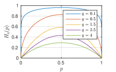
Figure 6: Tsallis $q$-entropy $H_{q}(p)$ for a binary clustering where $p$ is the relative size of one cluster. When $q$ is small, the $q$-entropy varies in bigger range.

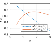
Let us focus on an example. Let $V$ be a reference clustering with 3 clusters of size 50 each, and let $U_{1}$ and $U_{2}$ be two clustering solutions with the same number of clusters and same cluster sizes. The contingency tables for $U_{1}$ and $U_{2}$ are shown on Figure 7.

		$V$
		50	50	50
	50	50	0	0
$U_{1}$	50	0	44	6
	50	0	6	44

		$V$
		50	50	50
	50	48	1	1
$U_{2}$	50	1	46	3
	50	1	3	46

Figure 7: AMI_q with small $q$ prefers the solution $U_{1}$ because there exist one pure cluster: i.e., there is one cluster which contains elements from only one cluster in the reference clustering $V$.

Given that both contingency tables have the same marginals, the only difference between AMI${}_{q}(U_{1},V)$ and AMI${}_{q}(U_{2},V)$ according to Eq. (11) lies in MI_q. Given that both solutions $U_{1}$ and $U_{2}$ are compared against $V$, the only term that varies in $\mbox{MI}_{q}(U,V)=H_{q}(V)-H_{q}(V|U)$ is $H_{q}(V|U)$. In order to identify the clustering solution that maximizes AMI_q we have to analyze the solution that decreases $H_{q}(V|U)$ the most. $H_{q}(V|U)$ is a weighted average of the entropies $H_{q}(V|u_{i})$ computed on the rows of the contingency table as shown in Eq. (5), and this is sensitive to values equal to 0. Given the bigger range of variation of $H_{q}$ for small $q$, small $q$ implies higher sensitivity to row entropies of 0. Therefore, small values of $q$ tends to decrease $H_{q}(V|U)$ much more if the clusters in the solution $V$ are pure: i.e., clusters contain elements from only one cluster in the reference clustering $V$. In other words, AMI_q with small $q$ prefers pure clusters in the clustering solution.

When the marginals in the contingency tables for two solutions are different, another important factor in the computation of AMI_q is the normalization coefficient $\frac{1}{2}(H_{q}(U)+H_{q}(V))$. Balanced solutions $V$ will be penalized more by AMI_q when $q$ is small. Therefore, AMI_q with small $q$ prefers unbalanced clustering solutions. To summarize, AMI_q with small $q$ such as AMI_0.5 or $\mbox{AMI}_{1}=\mbox{AMI}$ with Shannon’s entropy:

• Is biased towards pure clusters in the clustering solutions;

• Prefers unbalanced clustering solutions.

By contrary, AMI_q with bigger $q$ such as AMI_2.5 or $\mbox{AMI}_{2}=\mbox{ARI}$:

• Is less biased towards pure clusters in the clustering solution;

• Prefers balanced clustering solutions.

Given a reference clustering $V$, these biases can guide the choice of $q$ in AMI_q to identify more suitable clustering solutions.

4.1 Use AMI_q with small $q$ such as AMI_0.5 or $\mbox{AMI}_{1}=\mbox{AMI}$ when the reference clustering is unbalanced and there exist small clusters

If the reference cluster $V$ is unbalanced and presents small clusters, AMI_q with small $q$ might prefer more appropriate clustering solutions $U$. For example, in Figure 8 we show two contingency tables associated to two clustering solutions $U_{1}$ and $U_{2}$ for the reference clustering $V$ with 4 clusters of size $[10,10,10,70]$ respectively. When there exist small clusters in the reference $V$ their identification has to be precise in the clustering solution. The solution $U_{1}$ looks arguably better than $U_{2}$ because it shows many pure clusters. In this scenario we advise the use of AMI_0.5 or $\mbox{AMI}_{1}=\mbox{AMI}$ with Shannon’s entropy because it gives more weight to the clustering solution $U_{1}$.

		$V$
		$10$	$10$	$10$	$70$
$U_{1}$	$8$	$8$	$0$	$0$	$0$
	$7$	$0$	$7$	$0$	$0$
	$7$	$0$	$0$	$7$	$0$
	$78$	$2$	$3$	$3$	$70$

		$V$
		$10$	$10$	$10$	$70$
$U_{2}$	$10$	$7$	$1$	$1$	$1$
	$10$	$1$	$7$	$1$	$1$
	$10$	$1$	$1$	$7$	$1$
	$70$	$1$	$1$	$1$	$67$

Figure 8: AMI_q with small $q$ prefers the solution $U_{1}$ because its clusters are pure. When the reference clustering has small clusters their identification in the solution has to be precise. In this scenario we advise the use of AMI_0.5 or $\mbox{AMI}_{1}=\mbox{AMI}$.

4.2 Use AMI_q with big $q$ such as AMI_2.5 or $\mbox{AMI}_{2}=\mbox{ARI}$ when the reference clustering has big equal sized clusters

If $V$ is a reference clustering with big equal size clusters it is less crucial to have precise clusters in the solution. Indeed, precise clusters in the solution penalize the recall of clusters in the reference. In this case, AMI_q with bigger $q$ might prefer more appropriate solutions.

		$V$
		$25$	$25$	$25$	$25$
$U_{1}$	$17$	$17$	$0$	$0$	$0$
	$17$	$0$	$17$	$0$	$0$
	$17$	$0$	$0$	$17$	$0$
	$49$	$8$	$8$	$8$	$25$

		$V$
		$25$	$25$	$25$	$25$
$U_{2}$	$24$	$20$	$2$	$1$	$1$
	$25$	$2$	$20$	$2$	$1$
	$23$	$1$	$1$	$20$	$1$
	$28$	$2$	$2$	$2$	$22$

Figure 9: AMI_q with big $q$ prefers the solution $U_{2}$ because it is less biased to pure clusters in the solution. When the reference clustering has big equal sized clusters their precise identification is less crucial. In this scenario we advise the use of AMI_2.5 or $\mbox{AMI}_{2}=\mbox{ARI}$.

In Figure 9 we show two clustering solutions $U_{1}$ and $U_{2}$ for the reference clustering $V$ with 4 equal size clusters of size 25. The solution $U_{2}$ looks better than $U_{1}$ because each of its clusters identify more elements from particular clusters in the reference. Moreover, $U_{2}$ has to be preferred to $U_{1}$ because it consists in 4 equal sized clusters like for the reference clustering $V$. In this scenario we advise the use of AMI_2.5 or $\mbox{AMI}_{2}=\mbox{ARI}$ because it gives more importance to the solution $U_{2}$.

5 Standardization of Clustering Comparison Measures

Selection of the most similar partition $U$ to a reference partition $V$ is biased according to the chosen similarity measure, the number of sets $r$ in $U$, and their relative size. This phenomena is known as selection bias and it has been extensively studied in decision trees (White and Liu, 1994). Researchers in this area agree that in order to achieve unbiased selection of partitions, distribution properties of similarity measures have to be taken into account (Dobra and Gehrke, 2001; Shih, 2004; Hothorn et al., 2006). Using the permutation model, we proposed in Romano et al. (2014) to analytically standardize the Shannon MI by subtraction of its expected value and division by its standard deviation. In this Section, we discuss how to achieve analytical standardization of measures $S\in\mathcal{L}_{\phi}$.

In order to standardize measures $S(U,V)$ we must analytically compute their variance:

Lemma 3

If $S(U,V)\in\mathcal{L}_{\phi}$, when partitions $U$ and $V$ are random:

$$\mbox{\emph{Var}}(S(U,V))=\beta^{2}\Big{(}E\Big{[}\Big{(}\sum_{ij}\phi_{ij}(n_{ij})\Big{)}^{2}\Big{]}-\Big{(}\sum_{ij}E[\phi_{ij}(n_{ij})]\Big{)}^{2}\Big{)}\text{where }E\Big{[}\Big{(}\sum_{ij}\phi_{ij}(n_{ij})\Big{)}^{2}\Big{]}\text{is }$$

$$\sum_{ij}\sum_{n_{ij}}\phi(n_{ij})P(n_{ij})\cdot\Bigg{[} \phi_{ij}(n_{ij})+\sum_{i^{\prime}\neq i}\sum_{\tilde{n}_{i^{\prime}j}}\phi_{i^{\prime}j}(\tilde{n}_{i^{\prime}j})P(\tilde{n}_{i^{\prime}j})+$$

$$+\sum_{j^{\prime}\neq j}\sum_{\tilde{n}_{ij^{\prime}}}P(\tilde{n}_{ij^{\prime}})\Bigg{(}\phi_{ij^{\prime}}(\tilde{n}_{ij^{\prime}})+\sum_{i^{\prime}\neq i}\sum_{\tilde{\tilde{n}}_{i^{\prime}j^{\prime}}}\phi_{i^{\prime}j^{\prime}}(\tilde{\tilde{n}}_{i^{\prime}j^{\prime}})P(\tilde{\tilde{n}}_{i^{\prime}j^{\prime}})\Bigg{)}\Bigg{]}$$ (13)

where $n_{ij}\sim\mbox{\emph{Hyp}}(a_{i},b_{j},N)$, $\tilde{n}_{i^{\prime}j}\sim\mbox{\emph{Hyp}}(b_{j}-n_{ij},a_{i^{\prime}},N-a_{i})$, $\tilde{n}_{ij^{\prime}}\sim\mbox{\emph{Hyp}}(a_{i}-n_{ij},b_{j^{\prime}},N-b_{j})$, $\tilde{\tilde{n}}_{i^{\prime}j^{\prime}}\sim\mbox{\emph{Hyp}}(a_{i^{\prime}},b_{j^{\prime}}-\tilde{n}_{ij^{\prime}},N-a_{i})$ are hypergeometric random variables.

We can use the expected value to standardize $S\in\mathcal{L}_{\phi}$, such as generalized IT measures.

5.1 Standardization of Generalized IT Measures

The variance under the permutation model of generalized IT measures is:

Theorem 4

Using Eqs. (10) and (13) with $\phi_{ij}(\cdot)=(\cdot)^{q}$, when the partitions $U$ and $V$ are random:

1. $\mbox{\emph{Var}}(H_{q}(U,V))=\frac{1}{(q-1)^{2}N^{2q}}\Big{(}E[(\sum_{ij}n_{ij}^{q})^{2}]-(\sum_{ij}E[n_{ij}^{q}])^{2}\Big{)}$;

2. $\mbox{\emph{Var}}(\mbox{\emph{MI}}_{q}(U,V))=\mbox{\emph{Var}}(H_{q}(U,V))$

3. $\mbox{\emph{Var}}(\mbox{\emph{VI}}_{q}(U,V))=4\mbox{\emph{Var}}(H_{q}(U,V))$

We define the standardized version of the similarity measure $\mbox{MI}_{q}$ (SMI_q), and the standardized version of the distance measure VI_q (SVI_q) as follows:

$$\mbox{SMI}_{q}\triangleq\frac{\mbox{MI}_{q}-E[\mbox{MI}_{q}]}{\sqrt{\mbox{Var}(\mbox{MI}_{q})}},\quad\mbox{SVI}_{q}\triangleq\frac{E[\mbox{VI}]_{q}-\mbox{VI}_{q}}{\sqrt{\mbox{Var}(\mbox{VI}_{q})}},$$ (14)

As for the case of AMI_q and AVI_q, it turns out that SMI_q is equal to SVI_q:

Theorem 5

Using Eqs. (10) and (13) with $\phi_{ij}(\cdot)=(\cdot)^{q}$, the standardized MI${}_{q}(U,V)$ and the standardized VI${}_{q}(U,V)$ are:

$$\mbox{\emph{SMI}}_{q}(U,V)=\mbox{\emph{SVI}}_{q}(U,V)=\frac{\sum_{ij}n_{ij}^{q}-\sum_{ij}E[n_{ij}^{q}]}{\sqrt{E[(\sum_{ij}n_{ij}^{q})^{2}]-(\sum_{ij}E[n_{ij}^{q}])^{2}}}$$ (15)

This formula shows that we are interested in maximizing the difference between the sum of the cells of the actual contingency table and the sum of the expected cells under randomness. However, standardized measures differs from their adjusted counterpart because of the denominator, i.e. the standard deviation of the sums of the cells. Indeed, SMI_q and SVI_q measure the number of standard deviations MI_q and VI_q are from their mean.

There are some notable special cases for particular choices of $q$. Indeed, our generalized standardization of IT measures allows us to generalize also the standardization of pair-counting measures such as the Rand Index. To see this, let us define the Standardized Rand Index (SRI): $\mbox{SRI}\triangleq\frac{\textup{RI}-E[\textup{RI}]}{\sqrt{\textup{Var}(\textup{RI})}}$ and recall that the standardized $G$-statistic is defined as $\mbox{S}G\triangleq\frac{G-E[G]}{\sqrt{\textup{Var}(G)}}$ (Romano et al., 2014):

Corollary 2

It holds true that:
i) $\lim_{q\rightarrow 1}\mbox{\emph{SMI}}_{q}=\lim_{q\rightarrow 1}\mbox{\emph{SVI}}_{q}=\mbox{\emph{SMI}}=\mbox{\emph{SVI}}=\mbox{\emph{S}}G$ with Shannon entropy;
ii) $\mbox{\emph{SMI}}_{2}=\mbox{\emph{SVI}}_{2}=\mbox{\emph{SRI}}$.

Computational complexity:

The computational complexity of $\mbox{SVI}_{q}$ is dominated by computation of the second moment of the sum of the cells defined in Eq. (13):

Proposition 3

The computational complexity of $\mbox{\emph{SVI}}_{q}$ is $O(N^{3}c\cdot\max{\{c,r\}})$.

Note that the complexity is quadratic in $c$ and linear in $r$. This happens because of the way we decided to condition the probabilities in Eq. (13) in the proof of Lemma 3. With different conditions, it is possible to obtain a formula symmetric to Eq. (13) with complexity $O(N^{3}r\cdot\max{\{r,c\}})$ (Romano et al., 2014).

Statistical inference:

All IT measures computed on partitions can be seen as estimators of their true value computed using the random variables associated to the partitions $U$ and $V$. Therefore, SMI_q can be seen as a non-parametric test for independence for MI_q. We formalize this with the following proposition:

Proposition 4

The $p$-value associated to the test for independence between $U$ and $V$ using MI${}_{q}(U,V)$ is smaller than: $\frac{1}{1+\left(\textup{SMI}_{q}(U,V)\right)^{2}}$.

For example, if SMI_q is equal to 4.46 the associated $p$-value is smaller than 0.05. Neural time series data is often analyzed making use of the Shannon MI (e.g. see Chapter 29 in Cohen (2014)). It is common practice to test the independence of two time series by computing SMI via Monte Carlo permutations, sampling from the space of $N!$ cardinality. Our SMI_q can be effectively and efficiently used in this application because it is exact and obtains $O(N^{3}r\cdot\max{\{r,c\}})$ complexity.

5.2 Experiments on Selection Bias

In this section, we evaluate the performance of standardized measures on selection bias correction when partitions $U$ are generated at random and independently from the reference partition $V$. This hypothesis has been employed in previous published research to study selection bias (White and Liu, 1994; Frank and Witten, 1998; Dobra and Gehrke, 2001; Shih, 2004; Hothorn et al., 2006; Romano et al., 2014). In particular, we experimentally demonstrate that NMI_q is biased towards the selection of partitions $U$ with more clusters at any $q$. Therefore, in this scenario it is beneficial to perform standardization. Although the choice of whether performing standardization or not is dependent to the application (Romano et al., 2015). For example, it has been argued that in some cases the selection of clustering solutions should be biased towards solutions with the same number of clusters as in the reference (Amelio and Pizzuti, 2015). In this section we aim to show the effects of selection bias when clusterings are independent and that standardization helps in reducing it. Moreover, we will see in Section 5.3 that it is particularly important to correct for selection bias when the number of records $N$ is small.

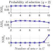
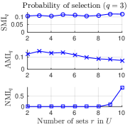
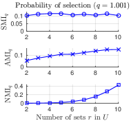
Given a reference partition $V$ on $N=100$ objects with $c=4$ sets, we generate a pool of random partitions $U$ with $r$ ranging from 2 to 10 sets. Then, we use NMI${}_{q}(U,V)$ to select the closest partition to the reference $V$. The plot at the bottom of Figure 10 shows the probability of selection of a partition $U$ with $r$ sets using NMI_q computed on 5000 simulations.

Figure 10: Selection bias towards partitions with different $r$ when compared to a reference $V$. The probability of selection should be uniform when partitions are random. Using SMI_q we achieve close to uniform probability of selection for $q$ equal to $1.001$, $2$ and $3$ respectively.

We do not expect any partition to be the best given that they are all generated at random: i.e., the plot is expected to be flat if a measure is unbiased. Nonetheless, we see that there is a clear bias towards partitions with 10 sets if we use NMI_q with $q$ respectively equal to 1.001, 2, or 3. We can see that the use of the adjusted measures such as AMI_q helps in decreasing this bias, in particular when $q=2$. On this experiment when $q=2$, baseline adjustment seems to be effective in decreasing the selection bias because the variance AMI${}_{2}=\mbox{ARI}$ is almost constant. However for all $q$, using SMI_q we obtain close to uniform probability of selection of each random partition $U$.

5.3 Large Number of Objects

It is likely to expect that the variance of generalized IT measures decreases when partitions are generated on a large number of objects $N$. Here we prove a general result about measures of the family $\mathcal{N}_{\phi}$.

Lemma 4

If $S(U,V)\in\mathcal{N}_{\phi}$, then $\lim_{N\rightarrow+\infty}\mbox{\emph{Var}}(S(U,V))=0$.

Given that generalized IT measures belong in the family $\mathcal{N}_{\phi}$, we can prove the following:

Theorem 6

It holds true that:

$$\lim_{N\rightarrow+\infty}\mbox{\emph{Var}}(H_{q}(U,V))=\lim_{N\rightarrow+\infty}\mbox{\emph{Var}}(\mbox{\emph{MI}}_{q}(U,V))=\lim_{N\rightarrow+\infty}\mbox{\emph{Var}}(\mbox{\emph{VI}}_{q}(U,V))=0$$ (16)

Therefore, SMI_q attains very large values when $N$ is large. In practice of course, $N$ is finite, so the use of SMI_q is beneficial. However, it is less important to correct for selection bias if the number of objects $N$ is big with regards to the number of cells in the contingency table in Table 2: i.e., when $\frac{N}{r\cdot c}$ is large. Indeed, when the number of objects is large AMI_q might be sufficient to avoid selection bias and any test for independence between partitions has high power. In this scenario, SMI_q is not needed and AMI_q might be preferred as it can be computed more efficiently.

6 Conclusion

In this paper, we computed the exact expected value and variance of measures of the family $\mathcal{L}_{\phi}$, which contains generalized IT measures. We also showed how the expected value for measures $S\in\mathcal{N}_{\phi}$ can be computed for large $N$. Using these statistics, we proposed AMI_q and SMI_q to adjust generalized IT measures both for baseline and for selection bias. AMI_q is a further generalization of well known measures for clustering comparisons such as ARI and AMI. This analysis allowed us to provide guidelines for their best application in different scenarios. In particular ARI might be used as external validation index when the reference clustering shows big equal sized clusters. AMI can be used when the reference clustering is unbalanced and there exist small clusters. The standardized SMI_q can instead be used to correct for selection bias among many possible candidate clustering solutions when the number of objects is small. Furthermore, it can also be used to test the independence between two partitions. All code has been made available online.

A Theorem Proofs

See 1

Proof 

$$\mbox{VI}_{q}(U,V) =2H_{q}(U,V)-H_{q}(U)-H_{q}(V)$$

$$=\frac{2}{q-1}\Big{(}1-\sum_{i=1}^{r}\sum_{j=1}^{c}\Big{(}\frac{n_{ij}}{N}\Big{)}^{q}\Big{)}-\frac{1}{q-1}\Big{(}1-\sum_{i=1}^{r}\Big{(}\frac{a_{i}}{N}\Big{)}^{q}\Big{)}-\frac{1}{q-1}\Big{(}1-\sum_{j=1}^{c}\Big{(}\frac{b_{j}}{N}\Big{)}^{q}\Big{)}$$

$$=\frac{1}{(q-1)N^{q}}\Big{(}\sum_{i=1}^{r}a_{i}^{q}+\sum_{j=1}^{c}b_{j}^{q}-2\sum_{i=1}^{r}\sum_{j=1}^{c}n_{ij}^{q}\Big{)}$$

When $q=2$, $\mbox{VI}_{2}(U,V)=\frac{1}{N^{2}}(\sum_{i}a_{i}^{2}+\sum_{j}b_{j}^{2}-2\sum_{i,j}n_{ij}^{2})=\frac{1}{N^{2}}\mbox{MK}(U,V)=\frac{N-1}{N}(1-\mbox{RI}(U,V))$.  

See 1

Proof  The expected value of $S(U,V)$ according to the hypergeometric model of randomness is $E[S(U,V)]=\sum_{\mathcal{M}}S(\mathcal{M})P(\mathcal{M})$ where $\mathcal{M}$ is a contingency table generated via permutations. This is reduced to $E[S(U,V)]=\sum_{\mathcal{M}}(\alpha+\beta\sum_{ij}\phi_{ij}(n_{ij}))P(\mathcal{M})=\alpha+\beta\sum_{\mathcal{M}}\sum_{ij}\phi_{ij}(n_{ij})P(\mathcal{M})$. Because of linearity of the expected value, it is possible to swap the summation over $\mathcal{M}$ and the one over cells obtaining $\alpha+\beta\sum_{ij}\sum_{n_{ij}}\phi_{ij}(n_{ij})P(n_{ij})=\alpha+\beta\sum_{ij}E[\phi_{ij}(n_{ij})]$ where $n_{ij}$ is a hypergeometric distribution with the marginals $a_{i}$, $b_{j}$, and $N$ as parameters, i.e. $n_{ij}\sim\mbox{Hyp}(a_{i},b_{j},N)$.  

See 1

Proof  The results easily follow from Lemma 1 and the hypothesis of fixed marginals.  

See 2

Proof  The using the upper bound $\frac{1}{2}(H_{q}(U)+H_{q}(V))$ to $\mbox{MI}_{q}$, $\mbox{AMI}_{q}$ and $\mbox{AVI}_{q}$ are equivalent. Therefore we compute $\mbox{AVI}_{q}$. The denominator is equal to $E[\mbox{VI}_{q}]=\frac{2}{(q-1)N^{q}}\Big{(}\frac{1}{2}(\sum_{i}a_{i}^{q}+\sum_{j}b_{j}^{q})-\sum_{i,j}E[n_{ij}^{q}]\Big{)}$. The numerator is instead $\frac{2}{(q-1)N^{q}}\Big{(}\sum_{ij}n_{ij}^{q}-\sum_{i,j}E[n_{ij}^{q}]\Big{)}$.  

See 1

Proof  Point i) follows from the limit of the $q$-entropy when $q\rightarrow 1$. Point ii) follows from:

$$\mbox{AVI}_{2}=\frac{E[\mbox{VI}_{2}]-\mbox{VI}_{2}}{E[\mbox{VI}_{2}]-\min{\mbox{VI}_{2}}}=\frac{\frac{N-1}{N}(\mbox{RI}-E[\mbox{RI}])}{\frac{N-1}{N}(\max{\mbox{RI}}-E[\mbox{RI}])}=\mbox{ARI}$$

 

See 2

Proof  The computation of $P(n_{ij})$ where $n_{ij}$ is a hypergeometric distribution $\mbox{Hyp}(a_{i},b_{j},N)$ is linear in $N$. However, the computation of the expected value $E[n_{ij}^{q}]=\sum_{n_{ij}}n_{ij}^{q}P(n_{ij})$ can exploit the fact that $P(n_{ij})$ are computed iteratively: $P(n_{ij}+1)=P(n_{ij})\frac{(a_{i}-n_{ij})(b_{j}-n_{ij})}{(n_{ij}+1)(N-a_{i}-b_{j}+n_{ij}+1)}$. We compute $P(n_{ij})$ only for  $\max{\{0,a_{i}+b_{j}-N\}}$. In both cases $P(n_{ij})$ can be computed in $O(\max{\{a_{i},b_{j}\}})$. We can compute all other probabilities iteratively as shown above in constant time. Therefore:

$$\sum_{i=1}^{r}\sum_{j=1}^{c}\left(O(\max{\{a_{i},b_{j}\}})+\sum_{n_{ij}=0}^{\min{\{a_{i},b_{j}\}}}O(1)\right) =\sum_{i=1}^{r}\sum_{j=1}^{c}O(\max{\{a_{i},b_{j}\}})=\sum_{i=1}^{r}O(\max{\{ca_{i},N\}})$$

$$=O(\max{\{cN,rN\}})=O(N\cdot\max{\{c,r\}})$$

 

See 2

Proof  $S(U,V)$ can be written as $\phi(\frac{n_{11}}{N},\dots,\frac{n_{ij}}{N},\dots,\frac{n_{rc}}{N})$. Let $\mathbf{X}=(X_{1},\dots,X_{rc})=(\frac{n_{11}}{N},\dots,\frac{n_{ij}}{N},\dots,\frac{n_{rc}}{N})$ be a vector of $rc$ random variables where $n_{ij}$ is a hypergeometric distribution with the marginals as parameters: $a_{i}$, $b_{j}$ and $N$. The expected value of $\frac{n_{ij}}{N}$ is $E[\frac{n_{ij}}{N}]=\frac{1}{N}\frac{a_{i}b_{j}}{N}$. Let $\boldsymbol{\mu}=(\mu_{1},\dots,\mu_{rc})=(E[X_{1}],\dots,E[X_{rc}])=(\frac{a_{1}}{N}\frac{b_{1}}{N},\dots,\frac{a_{i}}{N}\frac{b_{j}}{N},\dots,\frac{a_{r}}{N}\frac{b_{c}}{N})$ be the vector of the expected values. The Taylor approximation of $S(U,V)=\phi(\mathbf{X})$ around $\boldsymbol{\mu}$ is:

$$\phi(\mathbf{X})\simeq\phi(\boldsymbol{\mu})+\sum_{t=1}^{rc}(X_{t}-\mu_{t})\frac{\partial\phi}{\partial X_{t}}+\frac{1}{2}\sum_{t=1}^{rc}\sum_{s=1}^{rc}(X_{t}-\mu_{t})(X_{s}-\mu_{s})\frac{\partial^{2}\phi}{\partial X_{t}\partial X_{s}}+\dots$$

Its expected value is (see Section 4.3 of (Ang and Tang, 2006)):

$$E[\phi(\mathbf{X})]\simeq\phi(\boldsymbol{\mu})+\frac{1}{2}\sum_{t=1}^{rc}\sum_{s=1}^{rc}\mbox{Cov}(X_{t},X_{s})\frac{\partial^{2}\phi}{\partial X_{t}\partial X_{s}}+\dots$$

We just analyse the second order remainder given that it dominates the higher order ones. Using the Cauchy-Schwartz inequality we have that $|\mbox{Cov}(X_{t},X_{s})|\leq\sqrt{\mbox{Var}(X_{t})\mbox{Var}(X_{s})}$. Each $X_{t}$ and $X_{s}$ is equal to $\frac{n_{ij}}{N}$ for some indexes $i$ and $j$. The variance of each $X_{t}$ and $X_{s}$ is therefore equal to $\mbox{Var}(\frac{n_{ij}}{N})=\frac{1}{N^{2}}\frac{a_{i}b_{j}}{N}\frac{N-a_{i}}{N}\frac{N-b_{j}}{N-1}$. When the number of records is large also the marginals increase: $N\rightarrow+\infty\Rightarrow a_{i}\rightarrow+\infty$, and $b_{j}\rightarrow+\infty$ $\forall i,j$. However because of the permutation model, all the fractions $\frac{a_{i}}{N}$ and $\frac{b_{j}}{N}$ stay constant $\forall i,j$. Therefore, also $\boldsymbol{\mu}$ is constant. However, at the limit of large $N$, the variance of $\frac{n_{ij}}{N}$ tends to 0: $\mbox{Var}\Big{(}\frac{n_{ij}}{N}\Big{)}=\frac{1}{N}\frac{a_{i}}{N}\frac{b_{j}}{N}\Big{(}1-\frac{a_{i}}{N}\Big{)}\Big{(}1+\frac{1}{N-1}-\frac{b_{j}}{N}\Big{)}\rightarrow 0$. Therefore, at large $N$:

$$E[\phi(\mathbf{X})]\simeq\phi(\boldsymbol{\mu})=\phi\Big{(}\frac{a_{1}}{N}\frac{b_{1}}{N},\dots,\frac{a_{i}}{N}\frac{b_{j}}{N},\dots,\frac{a_{r}}{N}\frac{b_{c}}{N}\Big{)}$$

 

See 3

Proof  $E[H_{q}(U,V)]=\frac{1}{q-1}\Big{(}1-\sum_{ij}E\Big{[}\Big{(}\frac{n_{ij}}{N}\Big{)}^{q}\Big{]}\Big{)}$ and according to Lemma 2 for large $N$: $E[H_{q}(U,V)]\simeq\frac{1}{q-1}\Big{(}1-\sum_{ij}\Big{(}\frac{a_{i}}{N}\frac{b_{j}}{N}\Big{)}^{q}\Big{)}=\frac{1}{q-1}\Big{(}1-\sum_{i}\Big{(}\frac{a_{i}}{N}\Big{)}^{q}\sum_{j}\Big{(}\frac{b_{j}}{N}\Big{)}^{q}\Big{)}$. If we add an subtract $1-\sum_{i}\Big{(}\frac{a_{i}}{N}\Big{)}^{q}-\sum_{j}\Big{(}\frac{b_{j}}{N}\Big{)}^{q}$ in the parenthesis above:

$$E[H_{q}(U,V)] \simeq\frac{1}{q-1}\Big{(}1-\sum_{i}\Big{(}\frac{a_{i}}{N}\Big{)}^{q}\sum_{j}\Big{(}\frac{b_{j}}{N}\Big{)}^{q}$$

$$+1-\sum_{i}\Big{(}\frac{a_{i}}{N}\Big{)}^{q}-\sum_{j}\Big{(}\frac{b_{j}}{N}\Big{)}^{q}$$

$$-1+\sum_{i}\Big{(}\frac{a_{i}}{N}\Big{)}^{q}+\sum_{j}\Big{(}\frac{b_{j}}{N}\Big{)}^{q}\Big{)}$$

$$=\frac{1}{q-1}\Big{(}1-\sum_{i}\Big{(}\frac{a_{i}}{N}\Big{)}^{q}\Big{)}+\frac{1}{q-1}\Big{(}1-\sum_{j}\Big{(}\frac{b_{j}}{N}\Big{)}^{q}\Big{)}$$

$$+\frac{1}{q-1}\Big{(}-1-\sum_{i}\Big{(}\frac{a_{i}}{N}\Big{)}^{q}\sum_{j}\Big{(}\frac{b_{j}}{N}\Big{)}^{q}+\sum_{i}\Big{(}\frac{a_{i}}{N}\Big{)}^{q}+\sum_{j}\Big{(}\frac{b_{j}}{N}\Big{)}^{q}\Big{)}$$

$$=H_{q}(U)+H_{q}(V)+\frac{1}{q-1}\Big{(}\Big{(}1-\sum_{i}\Big{(}\frac{a_{i}}{N}\Big{)}^{q}\Big{)}\Big{(}\sum_{j}\Big{(}\frac{b_{j}}{N}\Big{)}^{q}\Big{)}\Big{)}$$

$$=H_{q}(U)+H_{q}(V)-(q-1)H_{q}(U)H_{q}(V)$$

Point ii) and iii) follow from Equations (6) and (7).  

See 3

Proof  The proof follows Theorem 1 proof in Romano et al. (2014). Using the properties of the variance we can show that $\mbox{Var}(S(U,V))=\beta^{2}\mbox{Var}(\sum_{ij}\phi_{ij}(n_{ij}))=\beta^{2}\Big{(}E[(\sum_{ij}\phi_{ij}(n_{ij}))^{2}]-(\sum_{ij}E[\phi_{ij}(n_{ij})])^{2}\Big{)}$. $(E[\sum_{ij}\phi_{ij}(n_{ij})])^{2}=(\sum_{ij}E[\phi_{ij}(n_{ij})])^{2}$ can be computed using Eq. (10). The first term in the sum is instead:

$$E[(\sum_{ij}\phi_{ij}(n_{ij}))^{2}]=\sum_{ij}\sum_{i^{\prime}j^{\prime}}E[\phi_{ij}(n_{ij})\phi_{i^{\prime}j^{\prime}}(n_{i^{\prime}j^{\prime}})]=\sum_{ij}\sum_{i^{\prime}j^{\prime}}\sum_{n_{ij}}\sum_{n_{i^{\prime}j^{\prime}}}\phi_{ij}(n_{ij})\phi_{i^{\prime}j^{\prime}}(n_{i^{\prime}j^{\prime}})P(n_{ij},n_{i^{\prime}j^{\prime}})$$

We cannot find the exact form of the joint probability $P(n_{ij},n_{i^{\prime}j^{\prime}})$ thus we rewrite it as $P(n_{ij})P(n_{i^{\prime}j^{\prime}}|n_{ij})=P(n_{ij})P(\tilde{n}_{i^{\prime}j^{\prime}})$. The random variable $n_{ij}$ is an hypergeometric distribution that simulates the experiment of sampling without replacement the $a_{i}$ objects in the set $u_{i}$ from a total of $N$ objects. Sampling one of the $b_{j}$ objects from $v_{j}$ is defined as success: $n_{ij}\sim\mbox{Hyp}(a_{i},b_{j},N)$. The random variable $\tilde{n}_{i^{\prime}j^{\prime}}$ has a different distribution depending on the possible combinations of indexes $i,i^{\prime},j,j^{\prime}$. Thus $E[(\sum_{ij}\phi_{ij}(n_{ij}))^{2}]$ is equal to:

$$\sum_{ij}\sum_{n_{ij}}\sum_{i^{\prime}j^{\prime}}\sum_{n_{i^{\prime}j^{\prime}}}\phi_{ij}(n_{ij})\phi_{i^{\prime}j^{\prime}}(n_{i^{\prime}j^{\prime}})P(n_{ij},n_{i^{\prime}j^{\prime}})=\sum_{ij}\sum_{n_{ij}}\phi_{ij}(n_{ij})P(n_{ij})\sum_{i^{\prime}j^{\prime}}\sum_{\tilde{n}_{i^{\prime}j^{\prime}}}\phi_{i^{\prime}j^{\prime}}(\tilde{n}_{i^{\prime}j^{\prime}})P(\tilde{n}_{i^{\prime}j^{\prime}})$$

which, by taking care of all possible combinations of $i,i^{\prime},j,j^{\prime}$, is equal to :

$$\sum_{ij}\sum_{n_{ij}}\phi_{ij}(n_{ij})P(n_{ij})\cdot\Bigg{[} \sum_{i^{\prime}=i,j^{\prime}=j}\sum_{\tilde{n}_{ij}}\phi_{ij}(\tilde{n}_{ij})P(\tilde{n}_{ij}) +\sum_{i^{\prime}\neq i,j^{\prime}=j}\sum_{\tilde{n}_{i^{\prime}j}}\phi_{i^{\prime}j}(\tilde{n}_{i^{\prime}j})P(\tilde{n}_{i^{\prime}j})$$ (17)

$$+\sum_{i^{\prime}=i,j^{\prime}\neq j}\sum_{\tilde{n}_{ij^{\prime}}}\phi_{ij^{\prime}}(\tilde{n}_{ij^{\prime}})P(\tilde{n}_{ij^{\prime}}) +\sum_{i^{\prime}\neq i,j^{\prime}\neq j}\sum_{\tilde{n}_{i^{\prime}j^{\prime}}}\phi_{i^{\prime}j^{\prime}}(\tilde{n}_{i^{\prime}j^{\prime}})P(\tilde{n}_{i^{\prime}j^{\prime}})\Bigg{]}$$ (18)

Case 1: $i^{\prime}=i\wedge j^{\prime}=j$

$P(\tilde{n}_{ij})=1$ if and only if $\tilde{n}_{ij}=n_{ij}$ and $0$ otherwise. This case produces the first term $\phi_{ij}(n_{ij})$ enclosed in square brackets.
Case 2: $i^{\prime}=i\wedge j^{\prime}\neq j$

In this case, the possible successes are the objects from the set $v_{j^{\prime}}$. We have already sampled $n_{ij}$ objects and we are sampling from the whole set of objects excluding the set $v_{j}$. Thus, $\tilde{n}_{ij^{\prime}}\sim\mbox{Hyp}(a_{i}-n_{ij},b_{j^{\prime}},N-b_{j})$.
Case 3: $i^{\prime}\neq i\wedge j^{\prime}=j$

This case is symmetric to the previous one where $a_{i^{\prime}}$ is now the possible number of successes. Therefore $\tilde{n}_{i^{\prime}j}\sim\mbox{Hyp}(b_{j}-n_{ij},a_{i^{\prime}},N-a_{i})$.
Case 4: $i^{\prime}\neq i\wedge j^{\prime}\neq j$

In order compute $P(\tilde{n}_{i^{\prime}j^{\prime}})$, we have to impose a further condition:

$$P(\tilde{n}_{i^{\prime}j^{\prime}})=\sum_{\tilde{n}_{ij^{\prime}}}P(\tilde{n}_{i^{\prime}j^{\prime}}|\tilde{n}_{ij^{\prime}})P(\tilde{n}_{ij^{\prime}})=\sum_{\tilde{n}_{ij^{\prime}}}P(\tilde{\tilde{n}}_{i^{\prime}j^{\prime}})P(\tilde{n}_{ij^{\prime}})$$

We are considering sampling the $a_{i^{\prime}}$ objects in $u_{i^{\prime}}$ from the whole set of objects excluding the $a_{i}$ objects from $u_{i}$. Just knowing that $n_{ij}$ objects have already been sampled from $u_{i}$ does not allow us to know how many objects from $v_{j^{\prime}}$ have also been sampled. If we know that $n_{ij^{\prime}}$ are the number of objects sampled from $v_{j^{\prime}}$, we know there are $b_{j^{\prime}}-n_{ij^{\prime}}$ possible successes and thus $\tilde{n}_{i^{\prime}j^{\prime}}|\tilde{n}_{ij^{\prime}}=\tilde{\tilde{n}}_{i^{\prime}j^{\prime}}\sim\mbox{Hyp}(a_{i^{\prime}},b_{j^{\prime}}-\tilde{n}_{ij^{\prime}},N-a_{i})$. So the last two terms in Eq. (18) can be put together:

$$\sum_{i^{\prime}=i,j^{\prime}\neq j}\sum_{\tilde{n}_{ij^{\prime}}}\phi_{ij^{\prime}}(\tilde{n}_{ij^{\prime}})P(\tilde{n}_{ij^{\prime}})+\sum_{i^{\prime}\neq i,j^{\prime}\neq j}\sum_{\tilde{n}_{i^{\prime}j^{\prime}}}\phi_{i^{\prime}j^{\prime}}(\tilde{n}_{i^{\prime}j^{\prime}})P(\tilde{n}_{i^{\prime}j^{\prime}})$$

$$=\sum_{j^{\prime}\neq j}\sum_{\tilde{n}_{ij^{\prime}}}\phi_{ij^{\prime}}(\tilde{n}_{ij^{\prime}})P(\tilde{n}_{ij^{\prime}})+\sum_{i^{\prime}\neq i,j^{\prime}\neq j}\sum_{\tilde{n}_{i^{\prime}j^{\prime}}}\phi_{i^{\prime}j^{\prime}}(\tilde{n}_{i^{\prime}j^{\prime}})\sum_{\tilde{n}_{ij^{\prime}}}P(\tilde{n}_{i^{\prime}j^{\prime}}|\tilde{n}_{ij^{\prime}})P(\tilde{n}_{ij^{\prime}})$$

$$=\sum_{j^{\prime}\neq j}\sum_{\tilde{n}_{ij^{\prime}}}\phi_{ij^{\prime}}(\tilde{n}_{ij^{\prime}})P(\tilde{n}_{ij^{\prime}})+\sum_{i^{\prime}\neq i,j^{\prime}\neq j}\sum_{\tilde{\tilde{n}}_{i^{\prime}j^{\prime}}}\phi_{i^{\prime}j^{\prime}}(\tilde{\tilde{n}}_{i^{\prime}j^{\prime}})\sum_{\tilde{n}_{ij^{\prime}}}P(\tilde{\tilde{n}}_{i^{\prime}j^{\prime}})P(\tilde{n}_{ij^{\prime}})$$

$$=\sum_{j^{\prime}\neq j}\sum_{\tilde{n}_{ij^{\prime}}}P(\tilde{n}_{ij^{\prime}})\phi_{ij^{\prime}}(\tilde{n}_{ij^{\prime}})+\sum_{j^{\prime}\neq j}\sum_{\tilde{n}_{ij^{\prime}}}P(\tilde{n}_{ij^{\prime}})\sum_{i^{\prime}\neq i}\sum_{\tilde{\tilde{n}}_{i^{\prime}j^{\prime}}}\phi_{i^{\prime}j^{\prime}}(\tilde{\tilde{n}}_{i^{\prime}j^{\prime}})P(\tilde{\tilde{n}}_{i^{\prime}j^{\prime}})$$

$$=\sum_{j^{\prime}\neq j}\sum_{\tilde{n}_{ij^{\prime}}}P(\tilde{n}_{ij^{\prime}})\Bigg{(}\phi_{ij^{\prime}}(\tilde{n}_{ij^{\prime}})+\sum_{i^{\prime}\neq i}\sum_{\tilde{\tilde{n}}_{i^{\prime}j^{\prime}}}\phi_{i^{\prime}j^{\prime}}(\tilde{\tilde{n}}_{i^{\prime}j^{\prime}})P(\tilde{\tilde{n}}_{i^{\prime}j^{\prime}})\Bigg{)}$$

By putting everything together we get that $E[(\sum_{ij}\phi_{ij}(n_{ij}))^{2}]$ is equal to:

$$\sum_{ij}\sum_{n_{ij}}\phi(n_{ij})P(n_{ij})\cdot\Bigg{[} \phi_{ij}(n_{ij})+\sum_{i^{\prime}\neq i}\sum_{\tilde{n}_{i^{\prime}j}}\phi_{i^{\prime}j}(\tilde{n}_{i^{\prime}j})P(\tilde{n}_{i^{\prime}j})+$$

$$+\sum_{j^{\prime}\neq j}\sum_{\tilde{n}_{ij^{\prime}}}P(\tilde{n}_{ij^{\prime}})\Bigg{(}\phi_{ij^{\prime}}(\tilde{n}_{ij^{\prime}})+\sum_{i^{\prime}\neq i}\sum_{\tilde{\tilde{n}}_{i^{\prime}j^{\prime}}}\phi_{i^{\prime}j^{\prime}}(\tilde{\tilde{n}}_{i^{\prime}j^{\prime}})P(\tilde{\tilde{n}}_{i^{\prime}j^{\prime}})\Bigg{)}\Bigg{]}$$

 

See 4

Proof  The results follow from Lemma 3, the hypothesis of fixed marginals and properties of the variance.  

See 5

Proof 
For $\mbox{SMI}_{q}$: the numerator is equal to $H_{q}(U,V)-E[H_{q}(U,V)]=\frac{1}{(q-1)N^{q}}\Big{(}\sum_{ij}n_{ij}^{q}-\sum_{i,j}E[n_{ij}^{q}]\Big{)}$. According Theorem 4, the denominator is instead:

$$\sqrt{\mbox{Var}(\mbox{MI}_{q}(U,V))}=\sqrt{\mbox{Var}(\mbox{H}_{q}(U,V))}=\frac{1}{(q-1)N^{q}}\sqrt{E[(\sum_{ij}n_{ij}^{q})^{2}]-(E[\sum_{ij}n_{ij}^{q}])^{2}}.$$

For $\mbox{SVI}_{q}$: the numerator is equal to $2H_{q}(U,V)-2E[H_{q}(U,V)]=\frac{2}{(q-1)N^{q}}\Big{(}\sum_{ij}n_{ij}^{q}-\sum_{i,j}E[n_{ij}^{q}]\Big{)}$. According Theorem 4, the denominator is instead:

$$\sqrt{\mbox{Var}(\mbox{VI}_{q}(U,V))}=\sqrt{4\mbox{Var}(\mbox{H}_{q}(U,V))}=\frac{2}{(q-1)N^{q}}\sqrt{E[(\sum_{ij}n_{ij}^{q})^{2}]-(E[\sum_{ij}n_{ij}^{q}])^{2}}.$$

Therefore, $\mbox{SMI}_{q}$ and $\mbox{SVI}_{q}$ are equivalent.  

See 2

Proof  Point i) follows from the limit of the $q$-entropy when $q\rightarrow 1$ and the linear relation to of $G$-statistic to MI: $G=2N\mbox{MI}$. Point ii) follows from:

$$\mbox{SVI}_{2}=\frac{E[\mbox{VI}_{2}]-\mbox{VI}_{2}}{\sqrt{\mbox{Var}(\mbox{VI}_{2})}}=\frac{\frac{N-1}{N}(\mbox{RI}-E[\mbox{RI}])}{\frac{N-1}{N}\sqrt{\mbox{Var}(\mbox{RI})}}=\mbox{SRI}$$

 

See 3

Proof  Each summation in Eq. (13) can be bounded above by the maximum value of the cell marginals and each sum can be done in constant time. The last summation in Eq. (13) is:

$$\sum_{j^{\prime}=1}^{c}\sum_{\tilde{n}_{ij^{\prime}}=0}^{\max{\{a_{i},b_{j^{\prime}}\}}}\sum_{i^{\prime}=1}^{r}\sum_{\tilde{\tilde{n}}_{i^{\prime}j^{\prime}}=0}^{\max{\{a_{i^{\prime}},b_{j^{\prime}}\}}}O(1) =\sum_{j^{\prime}=1}^{c}\sum_{\tilde{n}_{ij^{\prime}}=0}^{\max{\{a_{i},b_{j^{\prime}}\}}}O(\max{\{N,rb_{j^{\prime}}\}})$$

$$=\sum_{j^{\prime}=1}^{c}O(\max{\{a_{i}N,a_{i}rb_{j^{\prime}},b_{j^{\prime}}N,rb_{j^{\prime}}^{2}\}})$$

$$=O(\max{\{ca_{i}N,a_{i}rN,rN^{2}\}})$$

The above term is thus the computational complexity of the inner loop. Using the same machinery one can prove that:

$$\sum_{j=1}^{c}\sum_{i=1}^{r}\sum_{n_{ij}=0}^{\max{\{a_{i},b_{j}\}}}O(\max{\{ca_{i}N,a_{i}rN,rN^{2}\}})=O(\max{\{c^{2}N^{3},rcN^{3}\}})=O(N^{3}c\cdot\max{\{c,r\}})$$

 

See 4

Proof  Let MI${}^{0}_{q}$ be the random variable under the null hypothesis of independence between partitions associated to the test statistic MI${}_{q}(U,V)$. The $p$-value is defined as:

$$p\text{-value} =P\Big{(}\mbox{MI}^{0}_{q}\geq\mbox{MI}_{q}(U,V)\Big{)}=P\Big{(}\mbox{MI}^{0}_{q}-E[\mbox{MI}_{q}(U,V)]\geq\mbox{MI}_{q}(U,V)-E[\mbox{MI}_{q}(U,V)]\Big{)}$$

$$=P\Bigg{(}\frac{\textup{MI}^{0}_{q}-E[\textup{MI}_{q}(U,V)]}{\sqrt{\textup{Var}(\textup{MI}_{q}(U,V))}}\geq\frac{\textup{MI}_{q}(U,V)-E[\textup{MI}_{q}(U,V)]}{\sqrt{\textup{Var}(\textup{MI}_{q}(U,V))}}\Bigg{)}$$

$$=P\Bigg{(}\frac{\textup{MI}^{0}_{q}-E[\textup{MI}_{q}(U,V)]}{\sqrt{\textup{Var}(\textup{MI}_{q}(U,V))}}\geq\textup{SMI}_{q}(U,V)\Bigg{)}$$

Let $Z$ be the standardized random variable $\frac{\textup{MI}^{0}_{q}-E[\textup{MI}_{q}(U,V)]}{\sqrt{\textup{Var}(\textup{MI}_{q}(U,V))}}$, then using the one side Chebyshev’s inequality also known as the Cantelli’s inequality (Ross, 2012):

$$p\text{-value}=P(Z\geq\textup{SMI}_{q}(U,V))<\frac{1}{1+\Big{(}\textup{SMI}_{q}(U,V)\Big{)}^{2}}$$

 

See 4

Proof  Let $\mathbf{X}=(X_{1},\dots,X_{rc})=(\frac{n_{11}}{N},\dots,\frac{n_{ij}}{N},\dots,\frac{n_{rc}}{N})$ be a vector of $rc$ random variables where $n_{ij}$ is a hypergeometric distribution with the marginals as parameters: $a_{i}$, $b_{j}$ and $N$. Using the Taylor approximation (Ang and Tang, 2006) of $S(U,V)=\phi(\mathbf{X})$, it is possible to show that:

$$\mbox{Var}(\phi(\mathbf{X}))\simeq\sum_{t=1}^{rc}\sum_{s=1}^{rc}\mbox{Cov}(X_{t},X_{s})\frac{\partial\phi}{\partial X_{t}}\frac{\partial\phi}{\partial X_{s}}+\dots$$

Using the Cauchy-Schwartz inequality we have that $|\mbox{Cov}(X_{t},X_{s})|\leq\sqrt{\mbox{Var}(X_{t})\mbox{Var}(X_{s})}$. Each $X_{t}$ and $X_{s}$ is equal to $\frac{n_{ij}}{N}$ for some indexes $i$ and $j$. The variance of each $X_{t}$ and $X_{s}$ is therefore equal to $\mbox{Var}(\frac{n_{ij}}{N})=\frac{1}{N^{2}}\frac{a_{i}b_{j}}{N}\frac{N-a_{i}}{N}\frac{N-b_{j}}{N-1}$. When the number of records is large also the marginals increase: $N\rightarrow+\infty\Rightarrow a_{i}\rightarrow+\infty$, and $b_{j}\rightarrow+\infty$ $\forall i,j$. However because of the permutation model, all the fractions $\frac{a_{i}}{N}$ and $\frac{b_{j}}{N}$ stay constant $\forall i,j$. Therefore, at the limit of large $N$, the variance of $\frac{n_{ij}}{N}$ tends to 0: $\mbox{Var}\Big{(}\frac{n_{ij}}{N}\Big{)}=\frac{1}{N}\frac{a_{i}}{N}\frac{b_{j}}{N}\Big{(}1-\frac{a_{i}}{N}\Big{)}\Big{(}1+\frac{1}{N-1}-\frac{b_{j}}{N}\Big{)}\rightarrow 0$ and thus $\mbox{Var}(\phi(\mathbf{X}))$ tends to $0$.  

See 6

Proof  Trivially follows from Lemma 4.

References

• Aggarwal and Reddy (2013) Charu C. Aggarwal and Chandan K. Reddy. Data Clustering: Algorithms and Applications. CRC Press, 2013.
• Albatineh and Niewiadomska-Bugaj (2011) Ahmed N. Albatineh and Magdalena Niewiadomska-Bugaj. Correcting Jaccard and other similarity indices for chance agreement in cluster analysis. Advances in Data Analysis and Classification, 5(3):179–200, 2011.
• Albatineh et al. (2006) Ahmed N. Albatineh, Magdalena Niewiadomska-Bugaj, and Daniel Mihalko. On similarity indices and correction for chance agreement. Journal of Classification, 23(2):301–313, 2006.
• Amelio and Pizzuti (2015) Alessia Amelio and Clara Pizzuti. Is normalized mutual information a fair measure for comparing community detection methods? In Proceedings of the 2015 IEEE/ACM International Conference on Advances in Social Networks Analysis and Mining 2015, pages 1584–1585. ACM, 2015.
• Ang and Tang (2006) Alfredo H-S. Ang and Wilson H. Tang. Probability Concepts in Engineering: Emphasis on Applications to Civil and Environmental Engineering. John Wiley and Sons, 2006.
• Ben-Hur et al. (2001) Asa Ben-Hur, André Elisseeff, and Isabelle Guyon. A stability based method for discovering structure in clustered data. In Pacific symposium on biocomputing, volume 7, pages 6–17, 2001.
• Caruana et al. (2006) Rich Caruana, M Elhaway, Nam Nguyen, and Casey Smith. Meta clustering. In Data Mining, 2006. ICDM’06. Sixth International Conference on, pages 107–118. IEEE, 2006.
• Cohen (2014) Mike X Cohen. Analyzing neural time series data: theory and practice. MIT Press, 2014.
• Criminisi et al. (2012) Antonio Criminisi, Jamie Shotton, and Ender Konukoglu. Decision forests: A unified framework for classification, regression, density estimation, manifold learning and semi-supervised learning. Foundations and Trends in Computer Graphics and Vision, 7(2-3):81–227, 2012.
• Daróczy (1970) Zoltán Daróczy. Generalized information functions. Information and control, 16(1):36–51, 1970.
• Dobra and Gehrke (2001) Alin Dobra and Johannes Gehrke. Bias correction in classification tree construction. In Proceedings of the International Conference on Machine Learning, pages 90–97, 2001.
• Frank and Witten (1998) Eibe Frank and Ian H. Witten. Using a permutation test for attribute selection in decision trees. In Proceedings of the International Conference on Machine Learning, pages 152–160, 1998.
• Furuichi (2006) Shigeru Furuichi. Information theoretical properties of tsallis entropies. Journal of Mathematical Physics, 47(2):023302, 2006.
• Havrda and Charvát (1967) Jan Havrda and František Charvát. Quantification method of classification processes. concept of structural a𝑎a-entropy. Kybernetika, 3(1):30–35, 1967.
• Hothorn et al. (2006) Torsten Hothorn, Kurt Hornik, and Achim Zeileis. Unbiased recursive partitioning: A conditional inference framework. Journal of Computational and Graphical Statistics, 15(3):651–674, 2006.
• Hubert and Arabie (1985) Lawrence Hubert and Phipps Arabie. Comparing partitions. Journal of Classification, 2:193–218, 1985.
• Lei et al. (2014) Yang Lei, Nguyen Xuan Vinh, Jeffrey Chan, and James Bailey. Filta: Better view discovery from collections of clusterings via filtering. In Machine Learning and Knowledge Discovery in Databases, pages 145–160. Springer, 2014.
• Lopes et al. (2011) Fabrício M Lopes, Evaldo A de Oliveira, and Roberto M Cesar. Inference of gene regulatory networks from time series by Tsallis entropy. BMC systems biology, 5(1):61, 2011.
• Martins et al. (2009) André FT Martins, Noah A Smith, Eric P Xing, Pedro MQ Aguiar, and Mário AT Figueiredo. Nonextensive information theoretic kernels on measures. The Journal of Machine Learning Research, 10:935–975, 2009.
• Maszczyk and Duch (2008) Tomasz Maszczyk and Włodzisław Duch. Comparison of Shannon, Renyi and Tsallis entropy used in decision trees. In Artificial Intelligence and Soft Computing–ICAISC 2008, pages 643–651. Springer, 2008.
• Meilă (2007) Marina Meilă. Comparing clusterings – an information based distance. Journal of Multivariate Analysis, 98(5):873–895, 2007.
• Morey and Agresti (1984) Leslie C Morey and Alan Agresti. The measurement of classification agreement: an adjustment to the rand statistic for chance agreement. Educational and Psychological Measurement, 44(1):33–37, 1984.
• Müller et al. (2013) Emmanuel Müller, Stephan Günnemann, Ines Färber, and Thomas Seidl. Discovering multiple clustering solutions: Grouping objects in different views of the data. Tutorial at ICML, 2013. URL http://dme.rwth-aachen.de/en/DMCS.
• Rand (1971) William M Rand. Objective criteria for the evaluation of clustering methods. Journal of the American Statistical association, 66(336):846–850, 1971.
• Romano et al. (2014) Simone Romano, James Bailey, Vinh Nguyen, and Karin Verspoor. Standardized mutual information for clustering comparisons: One step further in adjustment for chance. In Proceedings of the 31st International Conference on Machine Learning (ICML-14), pages 1143–1151, 2014.
• Romano et al. (2015) Simone Romano, Nguyen Xuan Vinh, James Bailey, and Karin Verspoor. A framework to adjust dependency measure estimates for chance. arXiv preprint arXiv:1510.07786, 2015.
• Ross (2012) Sheldon Ross. A first course in probability. Pearson, 2012.
• Shih (2004) Y-S Shih. A note on split selection bias in classification trees. Computational statistics & data analysis, 45(3):457–466, 2004.
• Simovici (2007) Dan Simovici. On generalized entropy and entropic metrics. Journal of Multiple Valued Logic and Soft Computing, 13(4/6):295, 2007.
• Strehl and Ghosh (2003) Alexander Strehl and Joydeep Ghosh. Cluster ensembles—a knowledge reuse framework for combining multiple partitions. The Journal of Machine Learning Research, 3:583–617, 2003.
• Tsallis (1988) Constantino Tsallis. Possible generalization of Boltzmann-Gibbs statistics. Journal of statistical physics, 52(1-2):479–487, 1988.
• Tsallis et al. (2009) Constantino Tsallis et al. Introduction to Nonextensive Statistical Mechanics. Springer, 2009.
• Vila et al. (2011) Marius Vila, Anton Bardera, Miquel Feixas, and Mateu Sbert. Tsallis mutual information for document classification. Entropy, 13(9):1694–1707, 2011.
• Vinh et al. (2009) Nguyen Xuan Vinh, Julien Epps, and James Bailey. Information theoretic measures for clusterings comparison: is a correction for chance necessary? In Proceedings of the International Conference on Machine Learning, pages 1073–1080. ACM, 2009.
• Vinh et al. (2010) Nguyen Xuan Vinh, Julien Epps, and James Bailey. Information theoretic measures for clusterings comparison: Variants, properties, normalization and correction for chance. Journal of Machine Learning Research, 11:2837–2854, 2010.
• Vinh et al. (2014) Nguyen Xuan Vinh, Jeffrey Chan, Simone Romano, and James Bailey. Effective global approaches for mutual information based feature selection. In Proceedings of the 20th ACM SIGKDD international conference on knowledge discovery and data mining, pages 512–521. ACM, 2014.
• Warrens (2008) Matthijs J Warrens. On the equivalence of Cohen’s kappa and the Hubert-Arabie adjusted Rand index. Journal of Classification, 25(2):177–183, 2008.
• White and Liu (1994) Allan P. White and Wei Zhong Liu. Bias in information-based measures in decision tree induction. Machine Learning, pages 321–329, 1994.
• Wu et al. (2009) Junjie Wu, Hui Xiong, and Jian Chen. Adapting the right measures for k-means clustering. In Knowledge Discovery and Data Mining, pages 877–886, 2009.