Costly Circuits, Submodular Schedules:
Hybrid Switch Scheduling for Data Centers

Abstract

Hybrid switching – in which a high bandwidth circuit switch (optical or wireless) is used in conjunction with a low bandwidth packet switch – is a promising alternative to interconnect servers in today’s large scale data-centers. Circuit switches offer a very high link rate, but incur a non-trivial reconfiguration delay which makes their scheduling challenging. In this paper, we demonstrate a lightweight, simple and nearly-optimal scheduling algorithm that trades-off configuration costs with the benefits of reconfiguration that match the traffic demands. The algorithm has strong connections to submodular optimization, has performance at least half that of the optimal schedule and strictly outperforms state of the art in a variety of traffic demand settings. These ideas naturally generalize: we see that indirect routing leads to exponential connectivity; this is another phenomenon of the power of multi hop routing, distinct from the well-known load balancing effects.

1 Introduction

Modern data centers are massively scaling up to support demanding applications such as large-scale web services, big data analytics, and cloud computing. The computation in these applications is distributed across tens of thousands of interconnected servers. As the number and speed of servers increases, providing a fast, dynamic, and economic switching internconnect in data centers constitutes a topical networking challenging. Typically, data center networks use multi-rooted tree designs: the servers are arranged in racks and an Ethernet switch at top of the rack (ToR) connects the rack of servers to a one or more aggregation (or spine) layers. These designs use multiple paths between the ToRs to deliver uniform high bisection bandwidth, and consist of a large number of high speed electronic packet switches that provide fine-grained switching capabilities but at poor speed/cost ratios.

Recent work has proposed the use of high speed circuit switches based on optical [43, 14, 49] or wireless [25, 53, 23] links to interconnect the ToRs. These architecures enable a dynamic topology tuned to actual traffic patterns, and can provide a much higher aggregate capacity than a network of electronic switches at the same price point, consume significantly less power, and reduce cabling complexity. For instance, Farrington [13] reports 2.8$\times$, 6$\times$, 4.7$\times$ lower cost, power, and cabling complexity using optical circuit switching relative to a baseline network of electronic switches.

The drawback of circuit switches, however, is that their switching configuration time is much slower than electronic switches. Depending on the specific technology, reconfiguring the circuit switch can take a few milliseconds (e.g., for 3D MEMS optical circuit switches [43, 14, 49]) to 10s of microseconds (e.g., for 2D MEMs wavelength-selective switches [37]). During this reconfiguration period, the circuit switch cannot carry any traffic. By contrast, electronic switches can make per-packet switching decisions at sub-microsecond timescales. This makes the circuit switch suitable for routing stable traffic or bursts of packets (e.g., hundreds to thousands of packets at a time), but not for sporadic traffic or latency sensitive packets. A natural approach is then to have a hybrid circuit/packet switch architecture: the circuit switch can handle traffic flows that have heavy intensity but also require sparse connections, while a lower capacity packet switch handles the complementary (low intensity, but dense connections) traffic flows [14].

With this hybrid architecture, the relatively low intensity traffic is taken care of by the packet switch — switch scheduling here can be done dynamically based on the traffic arrival and is a well studied topic [34, 26, 33]. On the other hand, scheduling the circuit switch, based on the heavy traffic demand matrix, is still a fundamental unresolved question. Consider an architecture where a centralized scheduler samples the traffic requirements at each of the ToR ports at regular intervals ($W$, of the order of 100$\mu$s–1ms), and looks to find the schedule of circuit switch configurations over the interval of $W$ that is “matched" to the traffic requirements. The challenge is to balance the overhead of reconfiguration the circuits with the capability to be flexible and meet the traffic demand configuration.

The centralized scheduler must essentially decide a sequence of matchings between sending and receiving ToRs which the circuit switch then implements. For an optical circuit switch, for instance, the switch realizes the schedule by appropriately configuring its MEMs mirrors. As another example, in a broadcast-select optical ring architecture [7], the ToRs implement the controller’s schedule by tuning in to the appropriate wavelength to receive traffic from their matching sender as dictated by the schedule.

Hence, we need a scheduling algorithm that decides the state (i.e., matching) of the circuit switch at each time and also a routing protocol to decide on an appropriate route packets can take to reach their destination ToR port. This is a challenging problem and entails making several choices on: (a) number of matchings, (b) choice of matchings (switch configuration), (c) durations of the matchings and (d) the routing protocol, in each interval $W$. Mathematically, this leads to a well defined optimization problem, albeit involving both combinatorial and real-valued variables. Even special cases of this problem [29] are NP hard to solve exactly. Recent papers have proposed heuristic algorithms to address this scheduling problem. In [32] the authors present Solstice — a greedy perfect-matching based heuristic for a hybrid electrical-optical switch. Experimental evaluations show Solstice performing well over a simple baseline (where the schedules are provided by a truncated Birkoff-von Neumann decomposition of the traffic matrix), although no theoretical guarantees are presented. Indirect routing in a distributed setting, but without considerations of configuration switching costs, is studied in another recent work [7].

1.1 Our Contributions

We first focus on routing policies where packets are sent from the source port to the destination port only via a direct link connecting the two ports, leading to direct or single-hop routing. Our main result here is an approximately optimal, very simple and fast algorithm for computing the switch schedule in each interval. The algorithm, which we christen Eclipse, has a performance that is at least half that of optimal for every instance of the traffic demands, and experimentally shows a strict and consistent improvement over the state-of-the-art. A key technical contribution here is the identification of a submodularity structure [4] in the problem, which allows us to make connections to submodular function maximization and the circuit switch scheduling problem with reconfiguration delay.

Next, we consider routing polices where packets are allowed to reach their destination after (potentially) transiting through many intermediate ports, leading to indirect or multi-hop routing. This class of routing policies is motivated by our observation that if the number of matchings is limited, multi-hop routing can exponentially improve the reachability of nodes; a novel benefit of multi-hop routing distinct from the classical and well known load balancing effects [39, 46, 21]. We again identify submodularity in the problem, but the constraints for this submodular maximization problem are no longer linear and efficient solutions challenging to find. However, for the important special case where the sequence of switch configurations have already been calculated (and the indirect routing policy has to be decided) we propose a simple and fast greedy algorithm that is near optimal universally for all traffic requirements. Detailed experimental demonstrate strong improvements over direct routing, which are especially pronounced when the switch reconfiguration delays are relatively large.

The paper is organized as follows. In Section 2 the model, framework and the problem objective are formally stated along with a succinct summary of the state of the art. Section 3 focuses on direct routing and Section 4 on indirect routing. In Section 5 we present a detailed evaluation of the proposed algorithms on a variety of traffic inputs. Section 6 closes with a brief discussion. Technical aspects of the algorithm and its evaluation, including connections to submodularity and combinatorial optimization problems are deferred to the supplementary material.

2 System Model

In this section, we present our model for a hybrid circuit/packet-switched network fabric, and formally define our scheduling problem. Our model closely follows [32].

2.1 Hybrid Switch Model

We consider an $n$-port network where each port is simultaneously connected to a circuit switch and a packet switch. A set of nodes are attached to the ports and communicate over the network. The nodes could either be individual servers or “top-of-rack” switches.

We model the circuit switch as an $n\times n$ cross-bar comprising of $n$ input ports and $n$ output ports. At any point in time, each input port can send packets to at most one output port and each output port can receive packets from at most one input port over the circuit switch. The circuit switch can be reconfigured to change the input-output connections. We assume that the packets at the input ports are organized in virtual-output-queues [38] (VOQ) which hold packets destined to different output ports.

In practice, the circuit switch is typically an optical switch [43, 14, 49]. These switches have a key limitation: changing the circuit configuration imposes a reconfiguration delay during which the switch cannot carry any traffic. The reconfiguration delay can range from few milliseconds to 10s of microseconds depending on the technology [37, 31]. This makes the circuit switch suitable for routing stable traffic or bursts of packets (e.g., hundreds to thousands of packets at a time), but not for sporadic traffic or latency sensitive packets. Therefore, hybrid networks also use a (electrical) packet switch to carry traffic that cannot be handled by the circuit switch. The packet switch operates on a packet-by-packet basis, but has a much lower capacity than the circuit switch. For example, the circuit and packet switches might respectively run at 100Gbps and 10Gbps per port.

We divide time into slots, with each slot corresponding to a (full-sized) packet transmission time on the circuit switch. We consider a scheduling window of $W\in\mathbb{Z}$ time units. A central controller uses measurements of the aggregated traffic demand between different ports to determine a schedule for the circuit switch at the start of each scheduling window. The schedule comprises of a sequence of configurations and how long to use each configuration ($\S$2.3). We assume that the delay for each reconfiguration is $\delta\in\mathbb{Z}$ time units.

2.2 Traffic Demand

Let $T\in\mathbb{Z}^{n\times n}$ denote the accumulated traffic at the start of a scheduling window. We assume $T$ is a feasible traffic demand, i.e., $T$ is such that $\sum_{j=1}^{n}T(i,j)\leq W$ and $\sum_{i=1}^{n}T(i,j)\leq W$ for all $i,j\in\{1,2,\ldots,n\}$. The $(i,j)$th entry of $T$ denotes the amount of traffic that is in the VOQ at node $i$ destined for node $j$.

We assume that the controller knows $T$. We also assume that non-zero entries in the traffic matrix $T$ are bounded as $2\delta\leq T(i,j)\leq\epsilon W$ for all $i,j\in[n]:T(i,j)>0$ and some parameter $0<\epsilon<1$. This is a mild condition because traffic between pairs of ports that is small relative to $\delta$ is better served by the packet switch anyway.

Previous measurement studies have shown that the inter-rack traffic in production data centers is sparse [32, 6, 2, 40]. Over short periods of time (e.g., 10s of milliseconds), most nodes communicate with only a small number of other nodes (e.g., few to low tens). Further, in many cases, a large fraction of the traffic is sent by a small fraction of “elephant” flows [2]. While our algorithms and analysis are general, it is important to note that such sparse traffic patterns are necessary for hybrid networks to perform well (especially with larger reconfiguration delay).

2.3 The Scheduling Problem

Given the traffic demand, $T$, our goal is to compute a schedule that maximizes the total amount of traffic sent over the circuit switch during the scheduling window $W$. This is desirable to minimize the load on the slower packet switch. In general, the scheduling problem involves two aspects:

1. Determining a schedule of circuit switch configurations: The algorithm must determine a sequence of circuit switch configurations: $(\alpha_{1},P_{1}),(\alpha_{2},P_{2}),\ldots,(\alpha_{k},P_{k}).$ Here, $\alpha_{i}\in\mathbb{Z}$ denotes the duration of the $i^{th}$ switch configuration, and $P_{i}$ is an $n\times n$ permutation matrix, where $P_{i}(s,t)=1$ if input port $s$ is connected to output port $t$ in the $i^{th}$ configuration. For a valid schedule, we must have $\alpha_{1}+\alpha_{2}+\ldots+\alpha_{k}+k\delta\leq W$ since the total duration of the configurations cannot exceed the scheduling window $W$.

2. Deciding how to route traffic: The simplest approach is to use only direct routes over the circuit switch. In other words, each node only sends traffic to destinations to which it has a direct circuit during the scheduling window. Alternatively, we can allow nodes to use indirect routes, where some traffic is forwarded via (potentially multiple) intermediate nodes before being delivered to the destination. Here, the intermediate nodes buffer traffic in their VOQs for transmission over a circuit in a subsequent configuration.

In the next section, we begin by formally defining the problem in the simpler setting with direct routing and developing an algorithm for this case. Then, in $\S$4, we consider the more general setting with indirect routing.

Remark 1. Prior work [32, 29] has considered the objective of covering the entire traffic demand in the least amount of time. For example, the ADJUST algorithm in [29] takes the traffic demand $T$ as input and computes a schedule $(\alpha_{1},P_{1}),\ldots,(\alpha_{k},P_{k})$ such that $\sum_{i=1}^{k}\alpha_{i}P_{i}\geq T$ and $\sum_{i=1}^{k}\alpha_{i}+k\delta$ is minimized. Our formulation (and solution) is more general, since an algorithm which maximizes throughput over a given time period can also be used to find the shortest duration to cover the traffic demand (e.g., via binary search).

2.4 Related Work

Before presenting the work in this paper, we briefly summarize related work on this topic. Scheduling in crossbar switches is a classical and well studied topic and traditionally it has been used to model the packet switch where the reconfiguration delay is very small. Hence the scheduling solutions proposed – ranging from centralized Birkhoff-von-Neumann decomposition scheduler [34] on one end to the decentralized load-balanced scheduler [9] on the other – did not account for reconfiguration delay. In a different context (satellite-switched time-division multiple access), works such as [20] computed schedules that minimized the number of matchings in the schedule.

With the proposals on hybrid circuit/packet switching systems [14, 49], simplified models that factor for the reconfiguration delay were considered. Early works often assumed the delay to be either zero [24] or infinity [45, 51]. The infinite delay setting corresponds to a problem where the number of matchings is minimized. However they still require $O(n)$ matchings. Moderate reconfiguration delays are considered in DOUBLE [45] and other algorithms such as  [17, 29, 52] that explicitly take reconfiguration delay into account. The algorithm ADJUST [29] minmizes the covering time but still requires around $n$ configurations. All of these algorithms do not benefit from sparse demands and continue to require $O(n)$ configurations [32]. In a complementary approach, [10] considers conditions on the input traffic matrix under which efficient polynomial time algorithms to compute the optimal schedule exists. Yet other approaches have been to introduce speedup [33], or randomization in the algorithms [19], however they dont address the basic optimization problem underlying this scenario head-on. Such is the goal of this paper.

The above algorithms are “batch” policies [47] in which each computational call returns a schedule for an entire window of time. Another research direction is to consider “dynamic” policies where scheduling decisions are made time-slot by time-slot. A variant of the well known MaxWeight algorithm is presented in [48] and is shown to be throughput optimal. Fixed-Frame MaxWeight (FFMW) is a frame based policy proposed in [30] and has good delay performance. However it requires the arrival statistics to be known in advance. A hysteresis based algorithm that adapts many previously proposed algorithms for crossbar switch scheduling is presented in [47]. All these algorithms require perfect queue state information at every instant.

3 Direct Routing

The centralized scheduler samples the ToR ports and arrives at the traffic demand (matrix) $T$ to be met in the upcoming slot. In this section, we develop an algorithm, named Eclipse, that takes the traffic demand, $T$, as input and computes a schedule of matchings (circuit configurations) and their durations to maximize throughput over the circuit switch; only direct routing of packets from source to destination ports are allowed here. Eclipse is fast, simple and nearly-optimal in every instance of the traffic matrix $T$. Towards a formal understanding of the notion of optimality, consider the following optimization problem:

$$\mathrm{maximize}\quad\left\|\min\left(\sum_{i=1}^{k}\alpha_{i}P_{i},T\right)\right\|_{1}$$ (1)

$$\mathrm{s.t.}\quad\alpha_{1}+\alpha_{2}+\ldots+\alpha_{k}+k\delta\leq W$$ (2)

$$k\in\mathbb{N},P_{i}\in\mathcal{P},\alpha_{i}\geq 0~{}\forall i\in\{1,2,\ldots,k\}$$ (3)

where $\mathbb{N}=\{1,2,\ldots\}$ and $\mathcal{P}$ is the set of permutation matrices.

This optimization problem is NP-hard [29], and recent work [32] in the literature has focused on heuristic solutions. Our proposed algorithm has some similarities to the prior work in [32] in that the matchings and their durations are computed successively in a greedy fashion. However, the algorithm is overall quite different in terms of both details and ideas; we uncover and exploit the underlying submodularity [41] structure inherent in the problem to design and analyze the algorithm in a principled way.

3.1 Intuition

Before a formal presentation and analysis of the algorithm, we begin with an intuitive and less-formal approach to how one might solve this optimization problem. Consider greedy algorithms with the template shown in Algorithm 1. The template starts with an empty schedule, and proceeds to add a new matching to the schedule in each iteration. This process continues until the total duration of the matchings exceeds the allotted time budget of $W$, at which point the algorithm terminates and outputs the schedule computed so far. In each iteration, the algorithm first picks the duration of the matching, $\alpha$. It then selects the maximum weight matching in the traffic graph whose edge weights are thresholded by $\alpha$ (i.e., edge weights $>\alpha$ are clipped to $\alpha$). The traffic graph is a bipartite graph between $n$ input and $n$ output vertices, with an edge of weight $T(i,j)$ between input node $i$ and output node $j$. It only remains to specify how to choose $\alpha$ in each iteration.

Input : Traffic demand $T$, reconfiguration delay $\delta$ and scheduling window size $W$

Output : Sequence of matchings and weights: $(\alpha_{1},P_{1}),\ldots,(\alpha_{k},P_{k})$

$\mathrm{sch}\leftarrow\{\}$ ;

  // schedule

$k\leftarrow 0$ ;

$T_{\mathrm{rem}}\leftarrow T$ ;

  // traffic remaining

while $\sum_{i=1}^{k}(\alpha_{i}+\delta)\leq W$ do

       $k\leftarrow k+1$;

       Decide on a duration $\alpha$ for the matching;

       $M\leftarrow\mathrm{argmax}_{M\in\mathcal{M}}\|\min(\alpha M,T_{\mathrm{rem}})\|_{1}$ ;

       $\mathrm{sch}\leftarrow\mathrm{sch}\cup\{(\alpha,M)\}$ ;

       $T_{\mathrm{rem}}\leftarrow T_{\mathrm{rem}}-\min(\alpha M,T_{\mathrm{rem}})$ ;

      

end while

if $\sum_{i=1}^{k}(\alpha_{i}+\delta)>W$ then

      $\mathrm{sch}\leftarrow\mathrm{sch}\backslash\{(\alpha,M)\}$;

      

end if

Algorithm 1 A general greedy algorithm template

Consider an exercise where we vary the matching duration $\alpha$ from $0$ to $W$ and compute the maximum weight matching in the thresholded traffic graph for each $\alpha$. For a typical traffic matrix, this results in a curve similar to the solid-blue line in Fig. 1. Notice that the value of the maximum weight matching is precisely equal to the sum-throughput that can be achieved in that round of the switch schedule. It is straightforward to see that the maximum weight matching curve has the following properties: (a) it is non-decreasing and (b) piecewise linear. These are explained as follows: when $\alpha$ is very small a lot of the edges in the traffic graph have a weight that is saturated at $\alpha$. Hence it is likely to find a perfect matching with total weight of $n\alpha$. As such the slope of the curve when $\alpha$ is small is $n$. However, as $\alpha$ becomes large there are increasingly fewer edges whose weights are saturated at $\alpha$ and, correspondingly, theslope reduces. When $\alpha$ is so large that all of the edge weights are strictly smaller than $\alpha$, then the value of the maximum weight matching does not change even with any further increase in $\alpha$ and the curve ultimately flattens out.

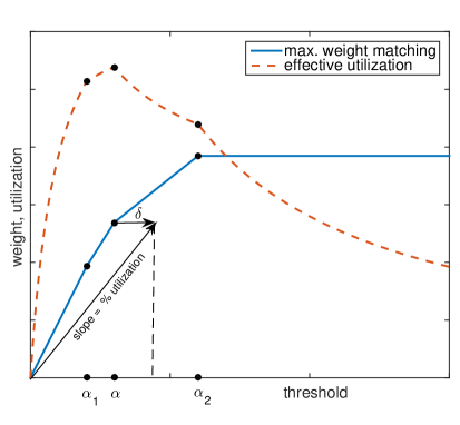
Figure 1: Throughput of max. weight matching as a function of threshold duration. The effective utilization curve of the matchings is also shown.

Two operating points of interest, considering Fig. 1, are (a) the largest $\alpha$ where the slope of the curve is maximum ($=n$ in the typical case where every ingress/egress port has traffic) and (b) the smallest $\alpha$ where the value of the maximum weight matching is the largest. These points have been denoted by $\alpha_{1}$ and $\alpha_{2}$ in Fig. 1 respectively. Setting $\alpha=\alpha_{1}$ is interesting because it results in a matching where the links are all fully utilized. For example, the Solstice algorithm presented in [32] implicitly adopts this operating point. On the other hand, $\alpha=\alpha_{2}$ gives a matching that achieves the largest possible sum-throughput in that round.

However we note that both choices of $\alpha$ are less than ideal for the following reasons. Recall that after every round of switching we incur a delay of $\delta$ time units. As such if the value of $\alpha_{1}$ is small (say $\O(\delta)$) in each round, then the number of matchings, and hence the time wasted due to the reconfiguration delay, becomes large. As a concrete example, consider the transpose of the traffic matrix $T_{1}=[A_{1}^{t}{\bf b}_{1}^{t}]$ where $A_{1}$ is a sparse $(n-1)\times n$ matrix and $\mathbf{b}=[2\delta,2\delta,\ldots,2\delta,0,0,\ldots,0]$ comprises of some $k$ entries of value $2\delta$ and $n-k$ entries of value 0. In other words, we are considering an input where a node or a collection of nodes have a large number of small flows to a particular node or vice-versa. For such an instance it is clear that if we insist on matchings with 100% utilized links, then the maximum duration of the matching is $2\delta$ (i.e., $\alpha_{1}=2\delta)$. Thus, continuing the process described in Algorithm 1 results in a sequence of $k$ matchings each of which is only $2\delta$ time units long. Hence in the worst case (if $k>1/(3\delta)$) about $1/3$rd of the entire scheduling window is wasted just due to reconfiguration delay limiting the maximum possible throughput to $2n/3$. On the other hand, if we had ignored the entries in $\mathbf{b}$, then we could have scheduled just $A_{1}$ achieving a total throughput of $n-2k\delta\approx n$ for large $n$. We point out that the phenomenon described above happens in a large family of instances, of which $T_{1}$ is a specific example. We also emphasize that such instances are pretty likely to occur in practice; for example, [40, Fig.5-b] shows traffic measurements in a Facebook datacenter where the interactions between Cache and Webservers lead to traffic matrices having this property.

Similarly for the operating point with $\alpha=\alpha_{2}$, consider the traffic matrix $T_{2}=\left[\begin{array}[]{cc}A_{2}&\mathbf{0}\\ \mathbf{0}&B_{2}\end{array}\right]$ where $A_{2}$ is a sparse $(n-2)\times(n-2)$ matrix and $B_{2}=\left[\begin{array}[]{cc}0&1\\ 1&0\end{array}\right].$ This is a diametrically opposite situation from $T_{1}$ where a small collection of nodes interact only amongst themselves with no interaction outside. Such a situation occurs, for example, in multi-tenant cloud-computing datacenters [42] where individual tenants run their jobs on small clusters of servers. In such a case, the value of the maximum weight matching can be maximum for a large $\alpha$. For $T_{2}$ the maximum value occurs at $\alpha=1-\delta$ (i.e., $\alpha_{2}=1-\delta$), resulting in a schedule with just one matching of duration $1-\delta$ and potentially missing a lot of traffic for $A_{2}$. For example, if $A_{2}$ is uniformly $k$-sparse, we miss out roughly $(k-1)n/k$ units of traffic. On the other hand, by choosing the duration of the matching to be $1/k-\delta$ in each step we can achieve a sum throughput of $n-O(\delta)\approx n$.

In scenarios exemplified by $T_{2}$, setting $\alpha=1$ is bad because the utilization of the resulting matching is poor, i.e., a vast majority of the matching links carry only a fraction of their capacity. This can be overcome by insisting that we choose only those matchings with utilization of at least 75% (say). However, in the case of $T_{1}$ we observe a poor performance in spite of all matchings having a utilization of 100%. The issue in this case is that the duration of the matchings are small compared to the reconfiguration delay. Hence to avoid this scenario we can insist on $\alpha\geq 20\delta$ (say) in Algorithm 1. Our first main observation is that both of the above heuristics are captured if we consider the effective utilization of the matchings. We define effective utilization as the ratio mwm$(\alpha)/(\alpha+\delta)$ where mwm$(\alpha)$ denotes the value of the maximum weight matching at $\alpha$. This ratio indicates the overall efficiency of a matching by including the reconfiguration delay into the duration. In Fig. 1 we plot the effective utilization of the matchings as the red-dotted curve. As can be seen there, the effective utilization at both $\alpha_{1}$ and $\alpha_{2}$ is suboptimal. We propose an algorithm that selects $\alpha$ to maximize effective utilization; a detailed description is deferred to Section 3.3.

The justification for selecting matchings according to the above is further reinforced by the submodularity structure of the problem (we discuss submodularity in Section 3.2). It turns out that for a certain class of submodular maximization problems with linear packing constraints, greedy algorithms take a form that precisely matches the intuitive thought process above: the proposed intuitively correct algorithm is borne out naturally from submodular combinatorial optimization theory. We briefly recall relevant aspects of submodularity and associated optimization algorithms next.

3.2 Submodularity

A set function $f:2^{[n]}\rightarrow\mathbb{R}$ is said to be submodular if it has the following property: for every $A,B\subseteq[n]$ we have $f(A\cup B)+f(A\cap B)\leq f(A)+f(B)$. Alternatively, submodular functions are also defined through the property of decreasing marginal values: for any $S,T$ such that $T\subseteq S\subseteq[n]$ and $j\notin S$, we have

$$f(S\cup\{j\})-f(S)\leq f(T\cup\{j\})-f(T).$$ (4)

The difference $f(S\cup\{j\})-f(S)$ is called the incremental marginal value of element $j$ to set $S$ and is denoted by $f_{S}(j)$. For our purpose we will only focus on submodular functions that are monotone and normalized, i.e., for any $S\subseteq T\subseteq[n]$ we have $f(S)\leq f(T)$ and further $f(\{\})=0$.

Many applications in computer science involve maximizing submodular functions with linear packing constraints. This refers to problems of the form:

$$\max f(S)\quad\text{s.t. }A\mathbf{x}_{S}\leq b\text{ and }S\subseteq[n]$$ (5)

where $A\in[0,1]^{m\times n},b\in[1,\infty)^{m}$ and $\mathbf{x}_{S}$ denotes the characteristic vector of the set $S$. Each of the $A_{ij}$’s is a cost incurred for including element $j$ in the solution. The $b_{i}$’s represent a total budget constraint. A well-known example of a problem in the above form is the Knapsack problem (the objective function in this case is in fact modular).

With the above background, we formulate the optimization problem under direct routing as one of submodular function maximization. Recall that for any given input traffic matrix $T$, the schedule that is computed is described by a sequence of matchings and corresponding durations. Consider the set $\mathcal{M}$ of all perfect matchings in the complete bipartite graph $K_{n\times n}$ with $n$ nodes in each partite. Then any round in the schedule is simply $(\alpha,P)\in\mathbb{Z}\times\mathcal{M}$. The key observation we make now is to view the schedules as a subset of $\mathbb{Z}\times\mathcal{M}$. Formally, define a switch schedule as any subset $\{(\alpha_{1},M_{1}),\ldots,(\alpha_{k},M_{k})\}$ of $\mathbb{Z}\times\mathcal{M}$. The objective function in our case is the sum-throughput defined as:

$$f(\{(\alpha_{1},M_{1}),\ldots,(\alpha_{k},M_{k})\})=\left\|\min\left\{\sum_{i=1}^{k}\alpha_{i}M_{i},T\right\}\right\|_{1}$$ (6)

where the minimum is taken entrywise and $\|\cdot\|_{1}$ refers to the entrywise $L_{1}$-norm of the matrix. We observe that the function $f$ is submodular, deferring the proof to the supplementary material.

Theorem 1.

The function $f:2^{\mathbb{Z}\times\mathcal{M}}\rightarrow\mathbb{R}$ defined by Equation (6) is a monotone, normalized submodular function.

We have established that optical switch scheduling under the sum-throughput metric is a submodular maximization problem. With this, we are ready to present a greedy algorithm that achieves a sum-throughput of at least a constant factor of the optimal algorithm for every instance of the traffic matrix.

3.3 Algorithm

Input : Traffic demand $T$, reconfiguration delay $\delta$ and scheduling window size $W$

Output : Sequence of matchings and weights: $(\alpha_{1},P_{1}),\ldots,(\alpha_{k},P_{k})$

$\mathrm{sch}\leftarrow\{\}$ ;

  // schedule

$k\leftarrow 0$ ;

$T_{\mathrm{rem}}\leftarrow T$ ;

  // traffic remaining

while $\sum_{i=1}^{k}(\alpha_{i}+\delta)\leq W$ do

       $k\leftarrow k+1$;

       $(\alpha,M)\leftarrow\mathrm{argmax}_{M\in\mathcal{M},\alpha\in\mathbb{R}_{+}}\frac{\|\min(\alpha M,T_{\mathrm{rem}})\|_{1}}{(\alpha+\delta)}$ ;

       $\mathrm{sch}\leftarrow\mathrm{sch}\cup\{(\alpha,M)\}$ ;

       $T_{\mathrm{rem}}\leftarrow T_{\mathrm{rem}}-\min(\alpha M,T_{\mathrm{rem}})$ ;

      

end while

if $\sum_{i=1}^{k}(\alpha_{i}+\delta)>W$ then

      $\mathrm{sch}\leftarrow\mathrm{sch}\backslash\{(\alpha,M)\}$;

      

end if

Algorithm 2 Eclipse: greedy direct routing algorithm

Algorithm 2 – Eclipse – captures our proposed solution under direct routing. Eclipse takes the traffic matrix $T$, the time window $W$ and reconfiguration delay $\delta$ as inputs, and computes a sequence of matchings and durations as the output. The algorithm proceeds in rounds (the “while loop"), where in each round a new matching is added to the existing sequence of matchings. The sequence terminates whenever the sum of the matching durations exceeds the allocated time window $W$ or whenever the traffic matrix $T$ is fully covered.

Consider any round $t$ in the algorithm; let $(\alpha_{1},M_{1}),\ldots,$ $(\alpha_{t-1},M_{t-1})$ denote the schedule computed so far in $t-1$ rounds (stored in variable $\mathtt{sch}$) and let $T_{\mathrm{rem}}(t)$ denote the amount of traffic yet to be routed. The matching that is selected in the $t$-th round is the one for which utilization is maximum. Utilization here refers to the percentage of the total matching capacity that is actually used. Mathematically, we choose an $(\alpha,M)$ pair such that $\|\min(\alpha M,T_{\mathrm{rem}})\|_{1}$ is maximized. In the supplementary material we have shown that that maxima occurs on the support of $T_{\mathrm{rem}}$. Hence this can be easily found by looking at the support of the (sparse) matrix $T_{\mathrm{rem}}$. We also propose a simple binary-search procedure, discussed in Algorithm 3, that finds a local maxima but performs extremely well in our evaluations (Section 5).

Input : Traffic demand $T$, reconfiguration delay $\delta$

Output : $(\alpha,M)\in\mathbb{R}_{+}\times\mathcal{M}$ such that $(\alpha,M)=\mathrm{argmax}_{M\in\mathcal{M},\alpha\in\mathbb{R}_{+}}\frac{\|\min(\alpha M,T)\|_{1}}{(\alpha+\delta)}$

$H\leftarrow$ distinct entries of $T$ sorted in ascending order;

$i_{\mathrm{lb}}\leftarrow 1$ and $i_{\mathrm{ub}}\leftarrow$ length$(H)$;

while $i_{\mathrm{lb}}<i_{\mathrm{ub}}$ do

       $i\leftarrow(i_{\mathrm{lb}}+i_{\mathrm{ub}})/2$ ;

       $T_{1}\leftarrow\min\{T,H(i)\}$ ;

        // thresholding $T$ to $H(i)$

       $T_{2}\leftarrow\min\{T,H(i+1)\}$ ;

       $v_{1}\leftarrow(\text{max. weight matching in }T_{1})/(H(i)+\delta)$ ;

       $v_{2}\leftarrow(\text{max. weight matching in }T_{2})/(H(i+1)+\delta)$ ;

       if $v_{1}<v_{2}$ then

            $i_{\mathrm{lb}}\leftarrow i$;

       else if $v_{1}>v_{2}$ then

            $i_{\mathrm{ub}}\leftarrow i$;

            

       else

            return $(H(i),$ max. weight matching in $T_{1})$;

       end if

      

end while

Algorithm 3 Finding the greedy maximum

As a concluding remark, we note that the constant $\epsilon$ in the approximation factor comes from the requirement that $\alpha+\delta\leq\epsilon W$ hold. We observe that this mild technical condition, required to show that Eclipse is a constant factor approximation of the optimal algorithm, has an added implication. Informally, it ensures that no single matching occupies the bulk of the scheduling window. This process of selecting a matching is repeated in each round until the sum-duration of the matchings exceed the scheduling window $W$, when the last chosen matching is discarded and the remaining set of matchings are returned. Eclipse is simple and also fast, a fact the following calculation demonstrates.

3.3.1 Complexity

We begin with the complexity of Algorithm 3. Since $i_{\mathrm{ub}}$ is no more than the number of distinct entries of $T$, we have $i_{\mathrm{ub}}\leq n^{2}$. In each iteration, the algorithm only considers entries of $H$ that have indices between $i_{\mathrm{lb}}$ and $i_{\mathrm{ub}}$. However, binary-search halves the effective size of $H$ (i.e., those numbers in $H$ with array indices $i_{\mathrm{lb}},i_{\mathrm{lb}+1},\ldots,i_{\mathrm{ub}}$), and the number of iterations of the while loop is bounded by $\log n^{2}=2\log n$. Within the while loop, computing the maximum weight matching can be done in $O(dn^{3/2}\log(W\epsilon))$ time (a basic fact of submodular optimization [12, 41]) where $dn$ is the number of edges in bipartite graph formed by $T$ (i.e., $d$ is the average sparsity) . Further $(1-\epsilon)$ approximate maximum weight matching can be computed in $O(dn\epsilon^{-1}\log\epsilon^{-1})$ [11], and efficient implementations in practice have been studied extensively in the literature [35, 36, 15]. Hence the overall time complexity is $O(dn^{3/2}\log n\log(W\epsilon))$. Now, in Algorithm 2 the number of iterations in the while loop is bounded by $W/\delta$. As such the total complexity of the algorithm is $\tilde{O}(dn^{3/2}\frac{W}{\delta})$. An exact search over the support of $T_{\mathrm{rem}}$ in the maximization step results in a overall complexity of $\tilde{O}(d^{2}n^{5/2}\frac{W}{\delta})$.

3.3.2 Approximation Guarantee

Since the proposed direct routing algorithm is connected to submodular maximization with linear constraints, we can adapt standard combinatorial optimization techniques to show an approximation factor of $1-1/e$. Let OPT denote the sum-throughput of the optimal algorithm for given inputs $T,\delta$ and $W$. Let ALG2 denote the sum-throughput achieved by Eclipse. We then have the following.

Theorem 2.

If the entries of $T$ are bounded by $\epsilon W+\delta$ then Eclipse approximates the optimal algorithm to within a factor of $1-1/e^{(1-\epsilon)}$, i.e.,

$$\mathtt{ALG2}\geq(1-1/e^{(1-\epsilon)})\mathtt{OPT}.$$ (7)

The proof of the above Theorem is deferred to the Appendix.

4 Indirect Routing

In the previous section, we focused on direct routing where packets are forwarded to their destination ports only if a link directly connecting the source port to the destination port appeared in the schedule – this is essentially a “single-hop” protocol. In this section, we explore allowing packets to be forwarded to (potentially) multiple intermediate ports before arriving at its final destination. In terms of implementing this more-involved protocol, we note that there is no extra overhead needed: the destination of any received packet is read first upon reception and since the queues are maintained on a per-destination basis at each ToR port, any received packet can be diverted to the appropriate queue. The key point of allowing indirect routing is the vastly increased range of ports that can be reached from a small number of matchings.

Consider Fig. 2 which illustrates a $6$-port network and a sequence of $3$ consecutive matchings in the schedule. In the first matching port 3 is connected to port 2; in the second matching it is connected to port 5 and so on. With direct routing, port 3 can only forward packets to port 2 in round 1, port 5 in round 2 and port 1 in round 3. In other words the set of egress ports reachable by port 3 is $\{2,3,5\}$. In the indirect routing framework of this section, port 3 can also forward packets to port 1. This can be achieved by first forwarding the packets to port 2 in the first round where the packets are queued. Then in the second round we let port 2 forward those packets to the destination port 3. Thus the reachability of the nodes is enhanced by allowing for indirect routing. Indirect routing can also be viewed as “multi-hop” routing.

Traditionally multi-hop routing has been used as a means of load balancing. This is known to be true in the context of networks such as the Internet where the benefits of “Valiant load-balancing" are legion [39, 46, 21]. The benefits of load balancing are also well known in the switching context – a classic example is the two-stage load-balancing algorithm in crossbar switches without reconfiguration delay [44]. The benefit of multi-hop routing in our context is markedly different: the reachability benefits of indirect routing are especially well suited to the setting where input ports are directly connected to only a few output ports due to the small number of matchings in the scheduling window. In fact, an elementary calculations shows that over a period of $k$ matchings in the schedule, indirect routing can allow a node to forward packets to $O(2^{k})$ other nodes, compared to only $O(k)$ nodes possible with direct routing. This is because of the recursion $f(k)=2f(k-1)+1$ where $f(k)$ denotes the number of nodes reachable by any node in $k$ rounds. If a node (say, node 1) can reach $f(k-1)$ nodes in $k-1$ rounds, then in the $k$th round (i) there is a new node directly connected to node 1 and (ii) each of the $f(k-1)$ nodes can be connected to a new node. Thus the number of nodes connected to node 1 in the $k$ -th round becomes $f(k-1)+(f(k-1)+1)$. Fig. 2 illustrates this phenomenon where reachability from node 6 is shown.

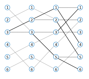
Figure 2: Reachability of nodes under multi-hop routing.

As a corollary we observe that $O(\log_{2}n)$ rounds of matchings are sufficient to reach all other nodes in a $n$-port network.

As in the direct routing case, computing the optimal schedule remains a challenging problem. While it is clear that we can achieve a performance at least as good as with direct routing, the gain is different for each instance of the traffic matrix – precisely quantifying the gain in an instance-specific way appears to be challenging. Our main result is that the submodularity property of the objective function continues to hold, provided the variables are considered in the appropriate format. Further, if we restrict some of the variables (the matchings and their durations), then there is also a natural, simple and fast greedy algorithm to compute the switching schedules and routing policies that is approximately optimal for each instance of the traffic matrix. This algorithm serves as a heuristic solution to the more general problem of jointly finding number of switchings, their durations, the switching schedules and routing policies. We present these results, following the same format as in the direct routing section, leaving numerical evaluations to a later section. We follow the model as discussed in Section 2.

4.1 Submodularity of objective function

We first adopt an alternative way of describing the switch schedule. Instead of specifying switch configurations round by round, and then specifying a multi-hop routing strategy in each round, we directly specify the path taken by each packet. The path-based formulation of multi-hop routing is well known in the problems of computing maximal flows in capacitated graphs and is crucial to understanding flow-cut gaps [50]; such a formulation serves us well in the causal structure of the routed traffic patterns that naturally occur here.

For simplicity we fix the number of rounds $k$ in the schedule. Consider a fully connected $k$-round time layered graph $G$: this graph consists of $k+1$ partites, $V_{0},V_{1},\ldots,V_{k}$, of $n$ nodes each. Nodes in each partite $i$ have directed edges to partite $i+1$ (such that the two partites form a complete bipartite graph). Let $\mathcal{P}$ denote the set of all paths in $G$ that begin at a node in $V_{0}$ and end at a node in $V_{k}$. Now, if we want to describe a multi-hop route for a packet in the system we can do it by choosing a $p\in\mathcal{P}$. If we are able to choose a path for every packet in the traffic matrix $T$, such that the union of the paths obey capacity constraints, then we would have succesfully specified a sequence of switch configurations and a routing policy for the schedule. Now, consider a function $f:2^{\mathbb{Z}\times\mathcal{P}}\rightarrow\mathbb{Z}$ defined by $f(\{(\beta_{1},p_{1}),\ldots,(\beta_{m},p_{m})\})\triangleq$

$$\sum_{i,j\in[n]}\min\left(\sum_{l=1}^{m}\beta_{l}\mathbf{1}_{\begin{subarray}{c}p_{l}(0)=i,\\ p_{l}(k+1)=j\end{subarray}},T_{ij}\right)$$ (8)

where $p(0)$ and $p(k+1)$ denote the starting and ending nodes of path $p$, and $\mathbf{1}_{\{\cdot\}}$ is the indicator function. Then the key observation is that $f$ is submodular.

Theorem 3.

The function $f:2^{\mathbb{Z}\times\mathcal{P}}\rightarrow\mathbb{Z}$ defined by Equation (8) is submodular.

The proof is similar to Theorem 1 and we omit it in the interests of space. So far we have not imposed any restrictions on the set of paths that we choose for the schedule. This can be incorporated in the form of constraints to the problem. Thus we are able to rephrase the objective as a constrained submodular maximization problem.

Constraints: Since we are only choosing weighted paths, we need to ensure that (i) the set of paths form a matching in each round and (ii) the total durations of the matching is at most $W-k\delta$. As such, we can write the following constraints for any subset $\{(\beta_{1},p_{1}),\ldots,(\beta_{m},p_{m})\}\in 2^{\mathbb{Z}\times\mathcal{P}}$ :

$$\sum_{\begin{subarray}{c}e:v\in e,\\ e\in E_{j}\end{subarray}}\mathbf{1}\left\{\sum_{i=1}^{m}\mathbf{1}_{\{e\in p_{i}\}}\beta_{i}>0\right\}\leq 1~{}\forall v\in V_{j-1},j\in[k]$$ (9)

$$\sum_{\begin{subarray}{c}e:v\in e,\\ e\in E_{j}\end{subarray}}\mathbf{1}\left\{\sum_{i=1}^{m}\mathbf{1}_{\{e\in p_{i}\}}\beta_{i}>0\right\}\leq 1~{}\forall v\in V_{j},j\in[k]$$ (10)

$$\sum_{j=1}^{k}\left(\left(\max_{e\in E_{j}}\sum_{i=1}^{m}\mathbf{1}_{\{e\in p_{i}\}}\beta_{i}\right)+\delta\right)\leq W$$ (11)

where $E_{j}$ stands for the edges between $V_{j-1}$ and $V_{j}$ in $G$. Hence we can express the problem as maximization of objective (8) subject to the constraints (9)– (11).

The key challenge here is that the constraints are nonlinear – it is not clear whether an efficient (approximation) algorithm exists. The nonlinearities appear only in the sense of membership tests and a corresponding thresholding function – so it is possible that an efficient nearly-optimal greedy algorithm exists; such a study is outside the scope of this manuscript. We do note, however, that for the special case in which the configurations are fixed and we only have to decide on the indirect routing policies, the constraints take on a linear form – in this setting, we are able to construct fast and efficient greedy algorithms. This case represents a composition of direct routing (where switch schedules are computed) and indirect routing (where the multi-hop routing policies are described), and is discussed next.

Multi-Hop Routing Policies: Consider a fixed sequence $(\alpha_{1},M_{1}),\ldots,(\alpha_{k},M_{k})$ of switch configurations and an input traffic demand matrix $T$. Let $G$ denote the time-layered graph obtained from the sequence of matchings, i.e., $G$ consists of $k+1$ partites $V_{0},\ldots,V_{k}$ with $n$ nodes each, and $M_{i}$ is the matching between partites $V_{i-1}$ and $V_{i}$ with edge weight $\alpha_{i}$ on the matching edges. In addition to the matching edges, there are also edges, with infinite edge weights, connecting the $j$-th nodes of $V_{i-1}$ and $V_{i}$ for all $j\in[n],i\in[k]$. In other words, $G$ is a time-layered graph whose edges are weighed according to the capacity available on the edges. Let $R(e)$ denote the capacity (= edge-weight) of edge $e\in G$. In this setting, the capacity constraints on the end-to-end paths are the sole constraints left in the optimization problem: in other words, the constraints in Equations 9 and 10 simplify to the following – we consider subsets $\{(\beta_{1},p_{1}),\ldots,(\beta_{m},p_{m})\}$ that obey:

$$\sum_{i=1}^{m}\beta_{i}\mathbf{1}_{\{e\in p_{i}\}}\leq R_{j}(e)~{}~{}\forall e\in R_{j},\forall j\in[k]$$ (12)

Notice that the constraints above have a linear form, and there are a total of $kn$ such constraints (one for each edge). Such a setting allows for a natural, simple, fast and nearly-optimal algorithm which we discuss below. Prior to that discussion, we remark that a naive approach to resolve the setting here is to formulate a linear program that maximizes the required objective. Indeed linear programming based approaches was the predominant technique used to solve this classical multicommodity flow problem [1, 22, 5]. However, despite many years of research in this direction the proposed algorithms were often too slow even for moderate sized instances [28]. Since then there has been a renewed effort in providing efficient approximate solutions to the multicommodity flow problem [18, 3]. The algorithm we propose is also a step in this direction, favoring efficiency over exactness of the solution. Note that in the path-formulation of the linear program there can be an exponential (in $k$) number of variables (for example, a schedule where node 1 is connected to node 2 and vice-versa in all the $k$ matchings has an exponential number of indirect paths from node 1 to 2). Thus there is no obvious efficient (exact) solution to this LP. On the other hand, the formulation we work with is able to handle this issue by appropriately weighing the edges and picking the path with the smallest weight; this latter step can be done efficiently – for example, using Dijkstra’s algorithm.

4.2 Algorithm

We propose an algorithm Eclipse++ directly motivated from [4], which presents a fast and efficient multiplicative weights algorithm for submodular maximization under linear constraints. The pseudocode has been given in Algorithm 4. The structure of Algorithm 4 is similar in spirit to direct-routing Algorithm 2 in the sense that (a) the algorithm proceeds in rounds, where one new path is added to the schedule in each round and (b) we select a path that offers the greatest utility per unit of cost incurred. However, unlike Algorithm 2 where there was only one linear constraint, we have multiple linear constraints now. This is addressed by assigning weights to the constraints and considering a linear combination of the costs as the true cost in each round. We describe the salient features of Algorithm 4 below.

Input : Traffic demand $T$, switch configurations with residue capacities $R_{1},\ldots,R_{k}$, update factor $\lambda$

Output : Sequence of paths and weights: $(\beta_{1},p_{1}),\ldots,(\beta_{m},p_{m})$

$\mathrm{sch}\leftarrow\{\}$ ;

  // schedule

$T_{\mathrm{rem}}\leftarrow T$ ;

  // traffic remaining

$w_{e}\leftarrow 1/R(e)$ for all $e\in E$;

$m\leftarrow 1$;

while $\sum_{e\in E}R(e)w_{e}\leq\lambda$ and $\|T_{\mathrm{rem}}\|_{1}>0$ do

       $(\beta_{m},p_{m})\leftarrow\mathrm{argmax}_{p\in\mathcal{P},\beta\in\mathbb{Z}}\frac{\min(\beta,T_{\mathrm{rem}}(p(0,p(k+1))}{\sum_{e\in E}\beta\mathbf{1}_{\{e\in p\}}w_{e}}$ ;

       $\mathrm{sch}\leftarrow\mathrm{sch}\cup\{(\beta_{m},p_{m})\}$ ;

       $T_{\mathrm{rem}}(p_{m}(0),p_{m}(k+1))\leftarrow T_{\mathrm{rem}}(p_{m}(0),p_{m}(k+1))-\beta$ ;

       $w_{e}\leftarrow w_{e}\lambda^{\beta_{m}\mathbf{1}_{\{e\in p\}}/R(e)}~{}~{}\forall e\in G$ ;

       $m\leftarrow m+1$;

      

end while

if $\sum_{i=1}^{m-1}\beta_{i}\mathbf{1}_{\{e\in p_{i}\}}\leq R(e)~{}~{}\forall e\in E$ then

      return sch

else

      return sch$\backslash(\beta_{m-1},p_{m-1})$

end if

Algorithm 4 Eclipse++ : greedy indirect routing algorithm

We begin by recalling that we have one constraint for each edge in the matchings for a total of $kn$ constraints. Let $w_{e}$ denote the weight assigned to the constraint involving edge $e$ and let $R(e)$ denote the capacity available with edge $e$. We set $w_{e}=1/R(e)$ for all $e$ initially, i.e., edges with a large capacity are assigned a small weight and vice-versa. Thus in addition to the time-layered capacity graph $G$, we can now have another graph $G_{w}$ (with same topology as $G$) whose edges are weighted by $w_{e}$. Now, for any path $p$ the “effective cost” of the path per unit of flow is simply the total cost of $p$ in $G_{w}$. Thus for the path $(\beta,p)$ carrying $\beta$ units of flow, the effective cost is given by $\sum_{e\in E}\beta w_{e}\mathbf{1}_{e\in p}$. On the other hand, the benefit we get due to adding path $(\beta,p)$ is given by $\min(\beta,T(p(0),p(k+1)))$ where $p(0)$ and $p(k+1)$ stand for the starting and terminating nodes along path $p$. Thus, the ratio $\frac{\min(\beta,T(p(0),p(k+1)))}{\sum_{e\in E}\beta w_{e}\mathbf{1}_{e\in p}}$ denotes the benefit of path $p$ per unit cost incurred. In Algorithm 4 we select $p$ such that the utility per unit cost is maximized.

Now, once we have selected a path $(\beta_{1},p_{1})$ in the first round, we update the weights $w_{e}$ on the edges. To do this we let a parameter $\lambda$ be input to the algorithm. Then, for each edge $e$ along the path $p$ the weights are updated as $w_{e}\leftarrow w_{e}\lambda^{\beta_{1}/R(e)}$; for the remaining edges the weights remain unchanged. Thus repeating the above iteratively until the while loop condition $\sum_{e\in E}R(e)w_{e}\leq\lambda$ becomes invalid, we get a schedule that is the output of the algorithm. It can also be shown that if the schedule returned sch violates any of the constraints (Equation (12)) then it must have happened at the very last iteration and hence we return a schedule with the last added path removed from it. A detailed analysis and correctness of the algorithm proposed is deferred to a full version of the paper and is omitted in this conference submission.

It only remains to show how the maximizer of

$$\frac{\min(\beta,T_{\mathrm{rem}}(p(0,p(k+1))}{\sum_{e\in E}\beta\mathbf{1}_{\{e\in p\}}w_{e}}$$ (13)

is computed efficiently in each round (first line inside the while loop). Recall that $G_{w}$ denotes the time-layered graph $G$ with edges weighted by $w_{e}$. Consider the set of shortest paths in $G_{w}$ (= smallest $w_{e}$-weighted path) from vertices in $V_{0}$ to vertices in $V_{k}$. Let $p^{*}$ denote the shortest among them. Then by setting $\beta^{*}\leftarrow T_{\mathrm{rem}}(p^{*}(0),p^{*}(k+1))$ we claim that Equation (13) is maximized. This is because,

$$\frac{\min(\beta,T_{\mathrm{rem}}(p(0,p(k+1))}{\sum_{e\in E}\beta\mathbf{1}_{\{e\in p\}}w_{e}}\leq\frac{\beta}{\sum_{e\in E}\beta\mathbf{1}_{\{e\in p\}}w_{e}}$$ (14)

$$\leq\frac{1}{\min\sum_{e\in E}\mathbf{1}_{\{e\in p\}}w_{e}}.$$ (15)

If $T_{\mathrm{rem}}(p^{*}(0),p^{*}(k+1))=0$ we proceed to the second smallest shortest path and so on. This allows a very efficient implementation of the internal maximization step.

4.2.1 Approximation Guarantee

We show, as in the direct-routing scenario, that Eclipse++ has a constant factor approximation guarantee. Specifically, for a fixed instance of the traffic matrix, let OPT and ALG4 denote the value of the objectives achieved by the optimal algorithm and Eclipse++, respectively. Let $\eta:=\max_{i,j\in[n],e\in E}T(i,j)/R(e)$. Then one can show that $\mathtt{ALG4}=\Omega(1/(nk)^{\eta})\mathtt{OPT}$ for $\lambda=e^{1/\eta}nk$; the proof is analogous to the direct-routing case, it follows [4, Theorem 1.1], and is deferred to a full version of this manuscript. Further, if $\eta=O(\epsilon^{2}/\log(nk))$ for some fixed $\epsilon>0$ then we get a approximation ratio of $(1-\epsilon)(1-1/e)$ by letting $\lambda=e^{\epsilon/(4\eta)}$ (this observation is inspired by [4, Theorem 1.2]). An interesting regime where this setting occurs is when the traffic matrices are dense with small skew. For example, we get a constant factor approximation if the sparsity of the traffic matrix grows logarithmically fast (or faster). This is in stark contrast to direct routing, where sparse matrices generally perform better.

4.2.2 Complexity

The proposed algorithm is simple and fast. In this subsection, we explicitly enumerate the time complexity of the full algorithm and show that the complexity is at most cubic in $n$ and nearly linear in $k$. Let $W$ denote a bound on the total incoming or outgoing traffic for a node. In each iteration of the while loop at least one unit of traffic is sent. Therefore there are at most $W$ iterations of the while loop. Now, in each iteration finding the shortest paths between nodes in $V_{0}$ to nodes in $V_{k}$ takes $kn^{2}(\log k+\log n)$ operations using Dijkstra’s algorithm [16]. Sorting the computed distances takes $kn^{2}(\log k+\log n)^{2}$ time and at most $n^{2}$ more operations to find a pair $i,j$ such that $T_{\mathrm{rem}}(i,j)>0$. Finally the weights update step takes $kn$ time. Therefore overall it takes $O(kn^{2}(\log k+\log n)^{2})$ time per iteration. Hence the time complexity of the complete algorithm is $O(Wkn^{3}(\log k+\log n)^{2})$.

5 Evaluation

Figure 3: Performance comparison of Eclipse under single-block inputs.

In this section, we compliment our analytical results with numerical simulations to explore the effectiveness of our algorithms and compare them to state-of-the-art techniques in the literature. We empirically evaluate both the direct routing algorithm (Eclipse; Algorithm 2) and the indirect routing algorithm (Eclipse++; Algorithm 4).

Metric: We consider the total fraction of traffic delivered via the circuit switch (sum-throughput) as the performance metric throughout this section.

Schemes compared. Our experiments compare Eclipse against two existing algorithms for direct routing:

Solstice [32]: This is the state-of-the-art hybrid circuit/packet scheduling algorithm for data centers. The key idea in Solstice is to choose matchings with 100% utilization. This is achieved by thresholding the demand matrix and selecting a perfect matching in each round. The algorithm presented in [32] tries to minimize the total duration of the window such that the entire traffic demand is covered. In this paper, we have considered a more general setting where the scheduling window $W$ is constrained. To compare against Solstice in this setting, we truncate its output once the total schedule duration exceeds $W$.

Truncated Birkhoff-von-Neumann (BvN) decomposition [8]: The second algorithm we compare against is the truncated BvN decomposition algorithm. BvN decomposition refers to expressing a doubly stochastic matrix as a convex combination of permutation matrices and this decomposition procedure has been extensively used in the context of packet switch scheduling [32, 27, 8]. However BvN decomposition is oblivious to reconfiguration delay and can produce a potentially large ($O(n^{2})$) number of matchings. Indeed, in our simulations BvN performs poorly.

Indirect routing is relatively new and to the best of our knowledge our work is the first to consider use of indirect routing for centralized scheduling. In our second set of simulations, we show that the benefits of indirect routing are in addition to the ones obtained from switch configurations scheduling. To this end, we compare Eclipse with Eclipse++ to quantify the additional throughput obtained by performing indirect routing (Algorithm 4) on a schedule that has been (pre)computed using Eclipse.

Traffic demands: We consider two classes of inputs: (a) single-block inputs and (b) multi-block inputs (explained in Section 5.1). Intuitively, single-block inputs are matrices which consist of one $n\times n$ ‘block’ that is sparse and skewed, and are similar to the traffic demands evaluated in the Solstice paper [32]. Multi-block inputs, on the other hand, denote traffic matrices that are composed of many sub-matrices each with disparate properties such as sparsity and skew.

Network size: The number of ports is fixed in the range of 50–200. We find that the relative performances stayed numerically stable over this range as well as for increased number of ports.

5.1 Direct Routing

While maintaining the sum-throughput as the performance metric, we vary the various parameters of the system model to gauge the performance in different situations.

Single-block Inputs

For a single-block input, our simulation setup consists of a network with $100$ ports. The link rate of the circuit switch is normalized to $1$, and the scheduling window length is also 1 $(W=1)$. We consider traffic inputs where the maximum traffic to or from any port is bounded by $W$. Further, we let the reconfiguration delay $\delta=W/100$. The traffic matrix is generated similar to [32] as follows. We assume $4$ large flows and $12$ small flows to each input or output port. The large flows are assumed to carry $70\%$ of the link bandwidth, while the small flows deliver the remaining $30\%$ of the traffic. To do this, we let each flow be represented by a random weighted permutation matrix, i.e., we have

$$T=\sum_{i=1}^{n_{L}}\frac{c_{L}}{n_{L}}P_{i}+\sum_{i^{\prime}=1}^{n_{S}}\frac{c_{S}}{n_{S}}P_{i^{\prime}}+N$$ (16)

where $n_{L}(n_{S})$ denotes the number of large (small) flows and $c_{L}(c_{S})$ denotes the total percentage of traffic carried by the large (small) flows. In this case, we have $n_{L}=4,n_{S}=12$ and $c_{L}=0.7,c_{S}=0.3$. Further, we have added a small amount of noise $N$ — additive Gaussian noise with standard deviation equal to $0.3\%$ of the link capacity — to the non-zero entries to introduce some perturbation. Each experiment below has been repeated 25 times.

Reconfiguration delay: In Fig. 3 we plot sum-throughput while varying the reconfiguration delay from $W/3200$ to $4W/100$. Ecliplse achieves a throughput of at least 90% for $\delta\leq W/100$. We observe Eclipse to be consistently better than Solstice although the difference is not pronounced until $\delta>W/100$. The BvN decomposition algorithm has a large throughput when the reconfiguration delay is small. As $\delta$ increases, it’s performance gradually worsens.

Skew: We control the skew by varying the ratio of the amount of traffic carried by small and large flows in the input traffic demand matrix ($c_{L}/c_{S}$ in Equation (16)). Fig. 3 captures the scenario where the percentage traffic carried by the small flows is varied from 5 to 75. We observe that Eclipse is very robust to skew variations and is able to consistently maintain a throughput of about 85%. Solstice has a slightly better performance at low skew (when small-flows carry $\sim 75\%$ of traffic); but overall, is dominated by Eclipse.

Sparsity: Finally, we tested the algorithms’ dependence on sparsity and plotted the results in Fig. 3. The total number of flows is varied from 4 to 32, while fixing the ratio of the number of large to small flows at 1:3. As the input matrix becomes less sparse, the performance of algorithms degrades as expected. However, for Eclipse, the reduction in the throughput is never more than 10% over the range of sparsity parameters considered. Solstice, on the other hand, is affected much more severely by decreased sparsity.

Figure 4: Performance comparison of Eclipse under multi-block inputs.

Figure 5: Performance of Eclipse++ and Eclipse. Here Eclipse++ uses the schedule computed by Eclipse.

Multi-Block Inputs

We now consider a more complex traffic model for a 200 node network with block diagonal inputs of the form

$$T=\left[\begin{array}[]{ccc}B_{1}&&\mathbf{0}\\ &\ddots&\\ \mathbf{0}&&B_{m}\end{array}\right]$$ (20)

where each of the component blocks $B_{1},B_{2},\ldots,B_{m}$ can have its own sparsity (number of flows) and skew (fraction of traffic carried by large versus small flows) parameters. The different blocks model the traffic demands of different tenants in a shared data center network such as a public cloud data center. To begin with, we consider inputs with two blocks $T=\left[\begin{array}[]{cc}B_{1}&\mathbf{0}\\ \mathbf{0}&B_{2}\end{array}\right]$ where $B_{1}$ is a $n_{1}\times n_{1}$ matrix with 4 large flows (carrying 70% of the traffic) and 12 small flows (carrying 30% of the traffic) and $B_{2}$ is a $(200-n_{1})\times(200-n_{1})$ matrix with uniform entries (up to sampling noise).

Size of block: Fig. 4 plots the throughput as the block size of $B_{2}$ is increased from 0 to 70. We observe a very pronounced difference in the performance of Eclipse and Solstice: Eclipse has roughly $1.5-2\times$ the performance of Solstice. These findings are in tune with the intuition discussed in Section 3.1 — the deteriorated performance of Solstice is due its insistance on perfect matchings in each round.

Reconfiguration delay: Fig. 4 plots throughput while varying the reconfiguration delay, for fixed size of $B_{2}$ to be $50\times 50$. As expected, the throughput of Solstice and Eclipse both degrade as the reconfiguration delay $\delta$ increases. However, Eclipse throughput degrades at a much slower rate than Solstice. The gap between the two is particularly pronounced for $\delta/W\geq 0.02$, a numerical value that is well within range of practical system settings.

Varying number of flows: In the final experiment we consider block diagonal inputs with 8 blocks of size $25\times 25$ each. Each block carries $10+\lfloor\sigma*(U-0.5))\rfloor$ equi-valued flows where $U\sim\text{unif }(0,1)$ and $\sigma$ is a parameter that controls the variation in the number of flows. When increasing $\sigma$ from 0 to 20 we see from Fig.4 that Eclipse is more or less able to sustain its throughput at close to 80%; whereas Solstice is significantly affected by the variation.

5.2 Indirect Routing

In this section, we consider a 50 node network with traffic matrices having varying number of large and small flows as before. We compare the performance of the direct routing algorithm and the indirect routing algorithm that is run on the schedule computed by Eclipse. To understand the benefits of indirect routing, we focus on the regime where the reconfiguration delay $\delta/W$ is relatively large and the scheduling window $W$ is relatively long compared to the traffic demand. This regime corresponds to realistic scenarios where the circuit switch is not fully utilized, but the reconfiguration delay is large. In this setting of relatively large $\delta/W$, switch schedules are forced to have only a small number of matchings, and indirect routing is critical to support (non-sparse) demand matrices. The following experiments numerically demonstrate the added gains of indirect routing.

Sparsity: Fig. 5 considers a demand with 5 large flows and number of small flows varying from 7 to 49. The large and the small flows each carry 50% of the traffic. We let $\delta=16W/100$ and consider a load of 20% (i.e., $W=5$, and traffic load at each port is 1). We observe that the performance of the Eclipse++ is roughly 10% better than Eclipse.

Load: As the network load increases (Fig. 5), we see that indirect routing becomes less effective. This is because at high load, the circuits do not have much spare capacity to support indirect traffic. However, at low to moderate levels of load, indirect routing provides a notable throughput gain over direct routing. For example, we see close to 20% improvement with Eclipse++ over Eclipse at 15% load.

Reconfiguration delay: Finally, we observe the effect of $\delta/W$ on throughput by varying $\delta$ from $3W/100$ to $21W/100$. At smaller values of reconfiguration delay $\delta$ both Eclipse and Eclipse++ are able to achieve near 100% throughput. With increasing $\delta$ both algorithms degrade with Eclipse++ providing an additional gain of roughly 20% over Eclipse.

6 Final Remarks

We have studied scheduling in hybrid switch architectures with reconfiguration delays in the circuit switch, by taking a fundamental and first-principles approach. The connections to submodular optimization theory allows us to design simple and fast scheduling algorithms and show that they are near optimal — these results hold in the direct routing scenario and indirect routing provided switch configurations are calculated separately. The problem of jointly deciding the switch configurations and indirect routing policies remains open. While submodular function optimization with nonlinear constraints is in general intractable, the specific constraints in Equations (9), (10) and (11) perhaps have enough structure that they can be handled in a principled way; this is a direction for future work.

In between the scheduling windows of $W$ time units, traffic builds up at the ToR ports. This dynamic traffic buildup is known locally to each of the ToR ports and perhaps this local knowledge can be used to pick appropriate indirect routing policies in a distributed, dynamic fashion. Such a study of indirect routing policies is initiated in a recent work [7], but this work omitted the switching reconfiguration delays. A joint study of distributed dynamic traffic scheduling in conjunction with a static schedule of switch configurations that account for reconfiguration delays is an interesting direction of future research.

7 Acknowledgments

The authors would like to thank Prof. Chandra Chekuri and Prof. R. Srikant for the many helpful discussions.

Appendix A Direct Routing - Proofs

In the following section we give the proof of Theorem 1.

A.1 Proof of Theorem 1

Proof.

Clearly $f(\{\})=0$. Also for any $S\subseteq S^{\prime}\in 2^{\mathbb{R}_{+}\times\mathcal{M}}$ we have

$$\min\left\{\sum_{(\alpha,M)\in S}\alpha M,T\right\} \leq\min\left\{\sum_{(\alpha,M)\in S^{\prime}}\alpha M,T\right\}$$

$$\Rightarrow f(S) \leq f(S^{\prime}).$$

Hence $f$ is normalized and monotone. The following identity holds for reals $a,b,c$: $\min(a+b,c)=\min(a,c)+\min(b,c-\min(a,c))$. Therefore for $S\in 2^{\mathbb{R}_{+}\times\mathcal{M}}$ and $(\alpha_{0},M_{0})\notin S$, we have

$$f(S\cup\{(\alpha,M)\})= \sum_{i,j\in[n]}\min\left\{\sum_{(\alpha,M)\in S}\alpha M+\alpha_{0}M_{0},T\right\}_{i,j}$$ (21)

$$= \sum_{i,j\in[n]}\left\{\min\left\{\sum_{(\alpha,M)\in S}\alpha M,T\right\}_{i,j}+\right.$$ (22)

$$\min\left\{\alpha_{0}M_{0},T\right. \left.-\min\left.\left\{\sum_{(\alpha,M)\in S}\alpha M,T\right\}\right\}_{i,j}\right\}$$ (23)

$$\Rightarrow f_{S}(\{(\alpha,M)\})= \left\|\min\left\{\alpha_{0}M_{0},T-\min\left\{\sum_{(\alpha,M)\in S}\alpha M,T\right\}\right\}\right\|_{1}$$ (24)

Now, for $S\subseteq S^{\prime}\in 2^{\mathbb{R}_{+}\times\mathcal{M}}$ and $(\alpha,M)\notin S^{\prime}$ since

$$T-\min\left\{\sum_{i\in S^{\prime}}\alpha_{i}M_{i},T\right\}\leq T-\min\left\{\sum_{i\in S}\alpha_{i}M_{i},T\right\}$$ (25)

together with Equation (24) this implies

$$f_{S^{\prime}}(\{(\alpha_{0},M_{0})\})\leq f_{S}(\{(\alpha_{0},M_{0})\}).$$ (26)

Hence $f$ is submodular. ∎

Next, we present the proof of Theorem 2.

A.2 Proof of Theorem 2

Proof.

Recall the submodular sum-throughput function $f$ defined in Equation (6). Let $\{(\alpha_{1},M_{1}),\ldots,(\alpha_{k},M_{k})\}$ be the schedule returned by Algorithm 2. Let $S_{i}=\{(\alpha_{1},M_{1}),$ $\ldots,(\alpha_{i},M_{i})\}$ denote the schedule computed at the end of $i$ iterations of the while loop and let $S^{*}$ denote the optimal schedule. Now, since in the $i+1$-th iteration $(\alpha_{i+1},M_{i+1})$ maximizes $\frac{\min(\alpha M,T_{\mathrm{rem}}(i+1))\|_{1}}{(\alpha+\delta)}=\frac{f_{S_{i}}(\{(\alpha,M)\})}{(\alpha+\delta)}$ we have for any $(\alpha,M)\notin S_{i}$,

$$\frac{f_{S_{i}}(\{(\alpha,M)\})}{(\alpha+\delta)} \leq\frac{f_{S_{i}}(\{(\alpha_{i+1},M_{i+1})\})}{(\alpha_{i+1}+\delta_{i+1})}$$ (27)

$$\Rightarrow f_{S_{i}}(\{(\alpha,M)\}) \leq\frac{(\alpha+\delta)}{(\alpha_{i+1}+\delta_{i+1})}f_{S_{i}}(\{(\alpha_{i+1},M_{i+1})\}).$$ (28)

Now consider $\mathtt{OPT}-f(S_{i})$ for some $i<k$. Since $f$ is monotone we have

$$\mathtt{OPT}-f(S_{i}) =f(S^{*})-f(S_{i})$$ (29)

$$\leq f(S_{i}\cup S^{*})-f(S_{i})$$ (30)

$$\leq\sum_{(\alpha,M)\in J^{*}}f_{S_{i}}(\{(\alpha,M)\})$$ (31)

$$\leq\sum_{(\alpha,M)\in J^{*}}\frac{(\alpha+\delta)}{(\alpha_{i+1}+\delta_{i+1})}f_{S_{i}}(\{(\alpha_{i+1},M_{i+1})\})$$ (32)

$$\leq\frac{W}{(\alpha_{i+1}+\delta_{i+1})}f_{S_{i}}(\{(\alpha_{i+1},M_{i+1})\})$$ (33)

where $J^{*}:=S^{*}\backslash S_{i}$ denotes the set of matchings that are present in the optimal solution but not in $S_{i}$, Equation (32) follows from Equation (28), and Equation (33) follows because $\sum_{(\alpha,M)\in J^{*}}(\alpha+\delta)\leq\sum_{(\alpha,M)\in S^{*}}(\alpha+\delta)\leq W$. Next, observe that

$$f(S_{i+1}) =f(S_{i})+f_{S_{i}}(\{(\alpha_{i+1},M_{i+1})\})$$ (34)

$$\Rightarrow\mathtt{OPT}-f(S_{i+1}) =\mathtt{OPT}-f(S_{i})-f_{S_{i}}(\{(\alpha_{i+1},M_{i+1})\})$$ (35)

$$\leq(\mathtt{OPT}-f(S_{i}))\left(1-\frac{(\alpha_{i+1}+\delta)}{W}\right)$$ (36)

$$\leq(\mathtt{OPT}-f(S_{0}))\prod_{i^{\prime}=1}^{i+1}\left(1-\frac{(\alpha_{i^{\prime}}+\delta)}{W}\right)$$ (37)

$$\leq\mathtt{OPT}\times e^{-\sum_{i^{\prime}=1}^{i+1}(\alpha_{i^{\prime}}+\delta)/W}$$ (38)

where Equation (36) follows from Equation (33) and Equation (38) follows because of the identity $1-x\leq e^{-x}$. Now, since after the $k$-th iteration the while loop terminates, this implies $\sum_{i^{\prime}=1}^{k}(\alpha_{i^{\prime}}+\delta)>W$. However, if the entries of the input traffic matrix $T$ are bounded by $\epsilon W+\delta$, then no matching has a duration longer than $\epsilon W$. In particular $\alpha_{k}+\delta\leq\epsilon W\Rightarrow\sum_{i^{\prime}=1}^{k-1}(\alpha_{i^{\prime}}+\delta)\geq W(1-\epsilon)$. Thus, setting $i=k-2$ in Equation (38) we have

$$\mathtt{OPT}-f(S_{k-1}) \leq\mathtt{OPT}\times e^{-\sum_{i^{\prime}=1}^{k-1}(\alpha_{i^{\prime}}+\delta)/W}$$ (39)

$$\leq\mathtt{OPT}\times e^{-(1-\epsilon)}$$ (40)

$$\Rightarrow\mathtt{OPT}-\mathtt{ALG2} \leq\mathtt{OPT}\times e^{-(1-\epsilon)}.$$ (41)

Hence we conclude $\mathtt{ALG2}\geq\mathtt{OPT}(1-e^{-(1-\epsilon)})$. ∎

A.3 Correctness

Consider traffic matrix $T\in\mathbb{Z}^{n\times n}$. Let $\mathcal{T}=\{T(i,j):i,j\leq[n]\}$ denote the distinct entries in the matrix $T$. Then, in the following, we show that the maximizer in

$$\max_{\alpha\in\mathbb{Z},M\in\mathcal{M}}\frac{\|\min(T,\alpha M)\|_{1}}{\alpha+\delta}$$ (42)

occurs for $\alpha\in\mathcal{T}$.

For any matching $M\in\mathcal{M}$ let us define $f_{M}(\alpha)\triangleq\|\min(\alpha M,T)\|_{1}$ and let $f(\alpha)\triangleq\max_{M\in\mathcal{M}}\frac{f_{M}(\alpha)}{\alpha+\delta}$

Proposition 1.

$f_{M}(\alpha)$ is (i) non-decreasing, (ii) piece-wise linear where the corner points are from $\mathcal{T}$ and (iii) concave.

Proof.

It is easy to see (i) because if $\alpha_{1}\leq\alpha_{2}$ then $\min(\alpha_{1}M,T)\leq\min(\alpha_{2}M,T)$ entrywise and hence $f_{M}(\alpha_{1})\leq f_{M}(\alpha_{2})$. To see (ii) consider any $t_{1}<t_{2}\in\mathcal{T}$ such that no other element of $\mathcal{T}$ is between $t_{1}$ and $t_{2}$. Then for $t_{1}\leq\alpha\leq t_{2}$ we have

$$f_{M}(\alpha)=\|\min(\alpha M,T)\|_{1}=\sum_{\begin{subarray}{c}(i,j)\in M\\ T(i,j)\leq t_{1}\end{subarray}}\min(\alpha,T(i,j))$$ (43)

$$+\sum_{\begin{subarray}{c}(i,j)\in M\\ T(i,j)\geq t_{1}\end{subarray}}\min(\alpha,T(i,j))$$ (44)

$$=\sum_{\begin{subarray}{c}(i,j)\in M\\ T(i,j)\leq t_{1}\end{subarray}}T(i,j)+\sum_{\begin{subarray}{c}(i,j)\in M\\ T(i,j)\geq t_{1}\end{subarray}}\alpha$$ (45)

$$=\sum_{\begin{subarray}{c}(i,j)\in M\\ T(i,j)\leq t_{1}\end{subarray}}T(i,j)+\left|\{(i,j)\in M:T(i,j)\geq t_{1}\}\right|\alpha$$ (46)

Thus $f_{M}(\cdot)$ is linear for $t_{1}\leq\alpha\leq t_{2}$ and (ii) follows. (iii) also follows from Equation (46) by observing that

$$\left|\{(i,j)\in M:T(i,j)\geq t_{1}\}\right|\geq\left|\{(i,j)\in M:T(i,j)\geq t_{2}\}\right|$$ (47)

for any $t_{1}<t_{2}\in\mathcal{T}$. Hence the slope of the piece-wise linear function $f_{M}(\alpha)$ is non-increasing as $\alpha$ increases. In other words, $f_{M}(\alpha)$ is concave. ∎

Proposition 2.

$\arg\max_{\alpha}\frac{f_{M}(\alpha)}{\alpha+\delta}\in\mathcal{T}$

Proof.

This follows from Proposition 1-(ii). Let $f_{M}(\alpha)$ be linear for $\alpha\in[t_{1},t_{2}]$. Then it can be written as $f_{M}(\alpha)=f_{M}(t_{1})+m(\alpha-t_{1})$ for some slope $m\geq 0$. Now, consider the derivation of the function $f_{M}(\alpha)/(\alpha+\delta)$ in the interval $[t_{1},t_{2}]$:

$$\frac{d}{d\alpha}\left(\frac{f_{M}(\alpha)}{\alpha+\delta}\right)=\frac{d}{d\alpha}\left(\frac{f_{M}(t_{1})+m(\alpha-t_{1})}{\alpha+\delta}\right)$$ (48)

$$=\frac{(\alpha+\delta)(m)-(f_{M}(t_{1})+m(\alpha-t_{1}))}{(\alpha+\delta)^{2}}$$ (49)

$$=\frac{\delta m-f_{M}(t_{1})+mt_{1}}{(\alpha+\delta)^{2}}$$ (50)

Note that the numerator of Equation (50) is independent of $\alpha$ and the denominator is strictly positive. Hence the sign (i.e., $>0,<0$ or $=0$) of the slope of $f_{M}(\alpha)/(\alpha+\delta)$ is the same in the interval $[t_{1},t_{2}]$. This proves that the maxima must occur at either of the extreme points $t_{1}$ or $t_{2}$. By Proposition 1-(ii) we know that the $f_{M}(\alpha)$ is piece-wise linear with the corner points from the set $\mathcal{T}$. Thus we can conclude that the maxima must occur at one of the points in $\mathcal{T}$. ∎

Theorem 4.

$\arg\max_{\alpha}f(\alpha)\in\mathcal{T}$

Proof.

This follows directly from Proposition 2. Notice that

$$\max_{\alpha}f(\alpha)=\max_{\alpha}\max_{M}\frac{f_{M}(\alpha)}{\alpha+\delta}$$ (51)

$$=\max_{M}\left(\max_{\alpha}\frac{f_{M}(\alpha)}{\alpha+\delta}\right)$$ (52)

But the maximizer of $f_{M}(\alpha)/(\alpha+\delta)$ belongs to $\mathcal{T}$ for any $M$. Hence we conclude that the maximizer of $f(\alpha)$ also belongs to $\mathcal{T}$. The Theorem follows. ∎

References

- [1] R. Ahuja, T. Magnanti, and J. Orlin. Network flows: theory, algorithms, and applications. Prentice Hall, 1993.
- [2] M. Alizadeh, A. Greenberg, D. A. Maltz, J. Padhye, P. Patel, B. Prabhakar, S. Sengupta, and M. Sridharan. Data center tcp (dctcp). SIGCOMM, 2011.
- [3] S. Arora, E. Hazan, and S. Kale. The multiplicative weights update method: a meta-algorithm and applications. Theory of Computing, 8(1):121–164, 2012.
- [4] Y. Azar and I. Gamzu. Efficient submodular function maximization under linear packing constraints. In Automata, Languages, and Programming, pages 38–50. Springer, 2012.
- [5] C. Barnhart and Y. Sheffi. A network-based primal-dual heuristic for the solution of multicommodity network flow problems. Transportation Science, 27(2):102–117, 1993.
- [6] T. Benson, A. Akella, and D. A. Maltz. Network traffic characteristics of data centers in the wild. In SIGCOMM, 2010.
- [7] Z. Cao, M. Kodialam, and T. Lakshman. Joint static and dynamic traffic scheduling in data center networks. In INFOCOM, 2014.
- [8] C.-S. Chang, W.-J. Chen, and H.-Y. Huang. Birkhoff-von neumann input buffered crossbar switches. In INFOCOM, 2000.
- [9] C.-S. Chang, D.-S. Lee, and Y.-S. Jou. Load balanced birkhoff-von neumann switches. In High Performance Switching and Routing, 2001 IEEE Workshop on, pages 276–280. IEEE, 2001.
- [10] A. Dasylva and R. Srikant. Optimal wdm schedules for optical star networks. IEEE/ACM Transactions on Networking (TON), 7(3):446–456, 1999.
- [11] R. Duan and S. Pettie. Linear-time approximation for maximum weight matching. J. ACM, 61(1):1:1–1:23, Jan. 2014.
- [12] R. Duan and H.-H. Su. A scaling algorithm for maximum weight matching in bipartite graphs. In SODA, 2012.
- [13] N. Farrington. Optics in data center network architecture. PhD thesis, Citeseer, 2012.
- [14] N. Farrington, G. Porter, S. Radhakrishnan, H. H. Bazzaz, V. Subramanya, Y. Fainman, G. Papen, and A. Vahdat. Helios: a hybrid electrical/optical switch architecture for modular data centers. SIGCOMM, 2011.
- [15] P. F. Felzenszwalb and R. Zabih. Dynamic programming and graph algorithms in computer vision. Pattern Analysis and Machine Intelligence, IEEE Transactions on, 33(4):721–740, 2011.
- [16] M. L. Fredman and R. E. Tarjan. Fibonacci heaps and their uses in improved network optimization algorithms. Journal of the ACM (JACM), 34(3):596–615, 1987.
- [17] S. Fu, B. Wu, X. Jiang, A. Pattavina, L. Zhang, and S. Xu. Cost and delay tradeoff in three-stage switch architecture for data center networks. In HPSR, 2013.
- [18] N. Garg and J. Koenemann. Faster and simpler algorithms for multicommodity flow and other fractional packing problems. SIAM Journal on Computing, 37(2):630–652, 2007.
- [19] P. Giaccone, B. Prabhakar, and D. Shah. Randomized scheduling algorithms for high-aggregate bandwidth switches. Selected Areas in Communications, IEEE Journal on, 21(4):546–559, 2003.
- [20] I. S. Gopal and C. K. Wong. Minimizing the number of switchings in an ss/tdma system. Communications, IEEE Transactions on, 33(6):497–501, 1985.
- [21] A. Greenberg, P. Lahiri, D. A. Maltz, P. Patel, and S. Sengupta. Towards a next generation data center architecture: scalability and commoditization. In Proceedings of the ACM workshop on Programmable routers for extensible services of tomorrow, pages 57–62. ACM, 2008.
- [22] M. Grötschel, L. Lovász, and A. Schrijver. Geometric algorithms and combinatorial optimization. Algorithms and combinatorics. Springer-Verlag, 1993.
- [23] N. Hamedazimi, Z. Qazi, H. Gupta, V. Sekar, S. R. Das, J. P. Longtin, H. Shah, and A. Tanwer. Firefly: a reconfigurable wireless data center fabric using free-space optics. In SIGCOMM, 2014.
- [24] T. Inukai. An efficient ss/tdma time slot assignment algorithm. Communications, IEEE Transactions on, 27(10):1449–1455, 1979.
- [25] S. Kandula, J. Padhye, and P. Bahl. Flyways to de-congest data center networks. 2009.
- [26] I. Keslassy, C.-S. Chang, N. McKeown, and D.-S. Lee. Optimal load-balancing. In INFOCOM, 2005.
- [27] I. Keslassy, M. Kodialam, T. Lakshman, and D. Stiliadis. On guaranteed smooth scheduling for input-queued switches. In INFOCOM, 2003.
- [28] T. Leighton, F. Makedon, S. Plotkin, C. Stein, É. Tardos, and S. Tragoudas. Fast approximation algorithms for multicommodity flow problems. Journal of Computer and System Sciences, 50(2):228–243, 1995.
- [29] X. Li and M. Hamdi. On scheduling optical packet switches with reconfiguration delay. Selected Areas in Communications, IEEE Journal on, 21(7):1156–1164, 2003.
- [30] Y. Li, S. Panwar, and H. J. Chao. Frame-based matching algorithms for optical switches. In High Performance Switching and Routing, 2003, HPSR. Workshop on, pages 97–102. IEEE, 2003.
- [31] H. Liu, F. Lu, A. Forencich, R. Kapoor, M. Tewari, G. M. Voelker, G. Papen, A. C. Snoeren, and G. Porter. Circuit switching under the radar with reactor. In NSDI, 2014.
- [32] H. Liu, M. K. Mukerjee, C. Li, N. Feltman, G. Papen, S. Savage, S. Seshan, G. M. Voelker, D. G. Andersen, M. Kaminsky, et al. Scheduling techniques for hybrid circuit/packet networks.
- [33] N. McKeown. The islip scheduling algorithm for input-queued switches. Networking, IEEE/ACM Transactions on, 7(2):188–201, 1999.
- [34] N. McKeown, A. Mekkittikul, V. Anantharam, and J. Walrand. Achieving 100% throughput in an input-queued switch. Communications, IEEE Transactions on, 47(8):1260–1267, 1999.
- [35] A. Mekkittikul and N. McKeown. A practical scheduling algorithm to achieve 100% throughput in input-queued switches. In INFOCOM, 1998.
- [36] S. Pettie and P. Sanders. A simpler linear time 2/3- approximation for maximum weight matching. Information Processing Letters, 91(6):271–276, 2004.
- [37] G. Porter, R. Strong, N. Farrington, A. Forencich, P. Chen-Sun, T. Rosing, Y. Fainman, G. Papen, and A. Vahdat. Integrating microsecond circuit switching into the data center. SIGCOMM, 2013.
- [38] B. Prabhakar and N. McKeown. On the speedup required for combined input-and output-queued switching. Automatica, 35(12):1909–1920, 1999.
- [39] M. O. Rabin. Efficient dispersal of information for security, load balancing, and fault tolerance. Journal of the ACM (JACM), 36(2):335–348, 1989.
- [40] A. Roy, H. Zeng, J. Bagga, G. Porter, and A. C. Snoeren. Inside the social network’s (datacenter) network. In SIGCOMM, 2015.
- [41] A. Schrijver. Combinatorial Optimization - Polyhedra and Efficiency. Springer, 2003.
- [42] A. Shieh, S. Kandula, A. Greenberg, and C. Kim. Seawall: performance isolation for cloud datacenter networks.
- [43] A. Singla, A. Singh, and Y. Chen. Osa: An optical switching architecture for data center networks with unprecedented flexibility. In NSDI, 2012.
- [44] R. Srikant and L. Ying. Communication Networks: An Optimization, Control and Stochastic Networks Perspective. Cambridge University Press, New York, NY, USA, 2014.
- [45] B. Towles and W. J. Dally. Guaranteed scheduling for switches with configuration overhead. Networking, IEEE/ACM Transactions on, 11(5):835–847, 2003.
- [46] L. G. Valiant. A bridging model for parallel computation. Communications of the ACM, 33(8):103–111, 1990.
- [47] C.-H. Wang and T. Javidi. Adaptive policies for scheduling with reconfiguration delay: An end-to-end solution for all-optical data centers. arXiv preprint arXiv:1511.03417, 2015.
- [48] C.-H. Wang, T. Javidi, and G. Porter. End-to-end scheduling for all-optical data centers. In Computer Communications (INFOCOM), 2015 IEEE Conference on, pages 406–414. IEEE, 2015.
- [49] G. Wang, D. G. Andersen, M. Kaminsky, K. Papagiannaki, T. Ng, M. Kozuch, and M. Ryan. c-through: Part-time optics in data centers. SIGCOMM, 2011.
- [50] D. P. Williamson and D. B. Shmoys. The design of approximation algorithms. Cambridge University Press, 2011.
- [51] B. Wu and K. L. Yeung. Nxg05-6: Minimum delay scheduling in scalable hybrid electronic/optical packet switches. In GLOBECOM, 2006.
- [52] B. Wu, K. L. Yeung, and X. Wang. Nxg06-4: Improving scheduling efficiency for high-speed routers with optical switch fabrics. In GLOBECOM, 2006.
- [53] X. Zhou, Z. Zhang, Y. Zhu, Y. Li, S. Kumar, A. Vahdat, B. Y. Zhao, and H. Zheng. Mirror mirror on the ceiling: Flexible wireless links for data centers. SIGCOMM, 2012.