Interfacial energies of systems of chiral molecules

Abstract.

We consider a simple model for the assembly of chiral molecules in two dimensions driven by maximization of the contact area. We derive a macroscopic model described by a parameter taking nine possible values corresponding to the possible minimal microscopic patterns and modulated phases of the chiral molecules. We describe the overall behaviour by means of an interaction energy of perimeter type between such phases. This energy is a crystalline perimeter energy, highlighting preferred directions for the interfaces between ensembles of molecules labelled by different values of the parameter.

Introduction

We consider a simple model of interaction between ensembles of two types of chiral molecules in two dimensions. The model has been described, together with other ones, in a paper by P. Szabelski and A. Woszczyk [15] (see also [3]).

Figure 1. Schematic picture of chiral molecules.

Such molecules are considered as occupying four sites of a square lattice with three points aligned in the vertical direction and one on one side in the two fashions represented in Fig. 1. We consider collections of molecules; i.e., collections of disjoint sets of points, each of which differs from one of the two just described by an integer translation. In [15] the energy of a molecule is expressed as

(0.1) $$\sum_{i=1}^{4}\sum_{j=1}^{4}s_{ij}\ ,$$

where $i$ parameterizes the four sites composing a molecule, and $j$ parameterizes the four neighbouring sites in ${\mathbb{Z}}^{2}$ of each element of the molecule; the value $s_{ij}$ equals $0$ if the site parameterized by $j$ belongs to some molecule (in particular it is $0$ if that site belongs to the same molecule) and equals $1$ if it does not belong to any other molecule. A discussion about chemical mechanisms for such energies can be found in [12, 13]. Our model can be viewed as a lattice system. Indeed, (up to an additive constant) the energy density $s_{ij}$ in (0.1) is nothing else than a ferromagnetic spin energy if we define the spin variable equal to $1$ on the sites of the molecules and equal to $-1$ on the remaining sites of a square lattice.

The objective of our analysis is to give a homogenized description of such a system through an approximate macroscopic energy which describes the typical collective mechanical behaviour of chiral molecules (see, e.g., [9, 10, 8]). The usual representation of the overall properties by a macroscopic spin variable or magnetization [12] is not possible, since the geometry of the system makes it of non-local type, as the fact that a site is occupied by a molecule of either type influences the system further than the nearest neighbours in a non-trivial way. Moreover, such a simple representation would integrate out the asymmetric microscopic behaviours of the molecules. For a better description, we have to define a new parameter that captures the relevant properties of the microscopic arrangement of the molecules, in the spirit of recent works on lattice systems with microstructure [1, 5].

In order to define an overall macroscopic parameter we first note that we may equivalently represent chiral molecules as unions of unit squares centered on points of a square lattice as in

Figure 2. Chiral molecules as union of squares.

Fig. 2. Correspondingly, the energy in (0.1) can be viewed as the length of the boundary of the molecule not in contact with any other molecule. The energy of a collection of molecules is then simply the total length of the boundary of the union of the molecules.

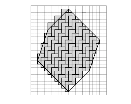
Figure 3. An ensemble of a single type of molecules minimizing the perimeter of their union, and its continuous approximation

We then examine the patterns of sets with minimal energy. In Fig. 3 we picture a set composed of a given number of one type of molecules minimizing its total boundary length. We first make the simple observation that, whenever this is allowed by boundary conditions, configuration of minimal energy replicate the pattern exhibited in that figure.

Figure 4. Patterns of configurations with zero energy in a square

More precisely, we prove that configurations with zero energy inside an open set either are the empty set (no molecule is present) or in the interior of that set they must correspond to a “striped” pattern of either of the two types in Fig. 4. These two patterns only are not sufficient to describe the behaviour of our energy, since the simultaneous presence of different translations of the same pattern will result in interstitial voids, and hence will have non-zero energy. We then remark that each pattern is four-periodic, and translating the pattern vertically (or horizontally) we obtain all different arrangements with zero energy. As a consequence, for each pattern we have four “modulated phases” corresponding to the four translations.

Figure 5. Four distinct modulated phases restricted to the same periodicity cell

In Fig. 5 we reproduce the unit cells of the different phases corresponding to the same pattern. In this way we have singled out eight different arrangements for the ground state, to which we have to add the trivial configuration with zero energy corresponding to the empty set. Note that the position of a single molecule determines the corresponding ground state.

In order to study the overall behaviour of a system of such chiral molecules, we follow a discrete-to-continuum approach, by scaling the system by a small parameter $\varepsilon$ and examine its behaviour as $\varepsilon\to 0$. We first give a notion of convergence of a family $E_{\varepsilon}$ of sets which are unions of scaled molecules of disjoint interior to a family $A_{1},\ldots,A_{8}$ by decomposing the set $E_{\varepsilon}$ into the sets $E_{1,\varepsilon},\ldots,E_{8,\varepsilon}$ defined as the union of the molecules corresponding to one of the eight modulated phases, respectively, and requiring that the symmetric difference between $E_{j,\varepsilon}$ and the corresponding $A_{j}$ tends to $0$ on each compact set of ${\mathbb{R}}^{2}$. We prove that this notion is indeed compact: if we have a family $E_{\varepsilon}$ of such sets with boundary with equibounded length, then, up to subsequences, it converges in the sense specified above. This is a non-trivial fact since it derives from a bound on the length of the boundary of the union of the sets $E_{j,\varepsilon}$, and not on each subfamily separately. We can nevertheless prove that each family $E_{j,\varepsilon}$ satisfies a similar bound on the length of the boundaries, and as a consequence is pre-compact as a family of sets of finite perimeter.

We then turn our attention to the description of the limit behaviour of the energies ${\mathcal{F}}_{\varepsilon}(E)={\mathcal{H}}^{1}(\partial E)$ defined on unions of scaled molecules with respect to the convergence $E_{\varepsilon}\to(A_{1},\ldots,A_{8})$ defined above. It is convenient to introduce the set $A_{0}$, complement of the union of $A_{1},\ldots,A_{8}$, which then corresponds to the limit of the complements of $E_{\varepsilon}$. In this way the completed family $\{A_{0},\ldots,A_{8}\}$ is a partition into sets of finite perimeter, for whose interfacial energies there exists an established variational theory [2]. We then represent the $\Gamma$-limit of the energies ${\mathcal{F}}_{\varepsilon}$ as

$${\mathcal{F}}(A_{0},\ldots,A_{8})=\sum_{i\neq j=0}^{8}\int_{\partial A_{i}\cap\partial A_{j}}f_{ij}(\nu^{i})d{\mathcal{H}}^{1},$$

where $f_{ij}$ is an interfacial energy and $\nu^{i}$ is the measure-theoretical normal to $\partial A_{i}$. The functions $f_{ij}(\nu)$ are represented by an asymptotic homogenization formula which describes the optimal way to microscopically arrange the molecules between two macroscopic phases $A_{i}$ and $A_{j}$ in a way to obtain an average interface with normal $\nu$. Note that this optimization process may be achieved by the use of molecules corresponding to phases other than $A_{i}$ and $A_{j}$.

This process can be localized, requiring that all molecules be contained in a set $\Omega$. In this case the same description holds, upon requiring that the partition satisfies $\bigcup_{j=1}^{8}A_{j}\subset\Omega$, or equivalently $A_{0}\supset{\mathbb{R}}^{2}\setminus\Omega$.

With the aid of the homogenization formula, we are able to actually compute the energy densities $f_{i}=f_{i0}=f_{0i}$; i.e., with one of the two phases corresponding to the empty set. In that case, $f_{i}$ is a crystalline perimeter energy, whose Wulff shape is an irregular hexagon corresponding to the continuous approximation of sets as in Fig. 3.

The paper is organized as follows. In Section 1 we introduce the necessary notation and prove the geometric Lemma 1.1 which characterizes configurations with zero energy on an open set. With the aid of that result in Section 2 we define the discrete-to continuous convergence of scaled families of chiral molecules to partitions into nine sets of finite perimeter, and prove that this is a compact convergence on families with equibounded energy. In Section 3 we first define the limit interfacial energy densities through an asymptotic homogenization formula and subsequently prove the $\Gamma$-convergence of the energies on scaled chiral systems to the energy defined through those interfacial energy densities. We then compute the energy densities and the related Wulff shapes when one of the phases is the empty set, and describe the treatment of anchoring boundary conditions. Finally, Section 4 is dedicated to generalization; in particular we remark that we may include a dependence on the type of chiral molecule, in which case optimal configuration may develop wetting layers. Another interesting observation is that we may consider as model energy the two-dimensional measure of ${\mathbb{R}}^{2}$ not occupied by a system of molecules (scaled by $1/\varepsilon$ for dimensional reasons when scaling the molecules) in place of the one-dimensional measure of their boundary. The analysis proceeds with minor changes except for the fact that the domain of the limit is restricted to the eight non-empty phases.

1. Geometric setting

We will consider ${\mathbb{R}}^{2}$ equipped with the usual scalar product, for which we use the notation $x\cdot y$. The Lebesgue measure of a set $E$ will be denoted by $|E|$; its $1$-dimensional Hausdorff measure by ${\mathcal{H}}^{1}(E)$. Given $U\subset{\mathbb{R}}^{2}$ and $x\in{\mathbb{R}}^{2}$, we denote by $U(x)$ the translation of $U$ by $x$; namely, $U(x):=x+U$.

We introduce the two fundamental chiral molecules as

$$R:=\big{(}[0,1]\times[0,3]\big{)}\cup\big{(}[1,2]\times[2,3]\big{)}\,,\qquad S:=\big{(}[-1,0]\times[0,3]\big{)}\cup\big{(}[-2,-1]\times[2,3]\big{)}\,,$$

corresponding to the two shapes in Fig. 2. We will consider sets that can be obtained as a union of integer translations of one of these two cells with pairwise disjoint interior. We denote by ${\mathcal{E}}$ the collection of families of sets defined as

$$\mathcal{E}:=\left\{\{E_{j}\}_{j}:E_{j}\in\{R(n),S(n):\,n\in{\mathbb{Z}}^{2}\},|E_{j}\cap E_{j^{\prime}}|=0\hbox{ if }j\neq j^{\prime}\right\}.$$

In this notation we do not specify the set of the indices $j$ since it will never be relevant in our arguments. We may also simply write $\{E_{j}\}$ in the place of $\{E_{j}\}_{j}$ if no ambiguity arises. Each set of $E_{j}$ will be referred to as a molecule.

We define ${\mathcal{A}}$ as the family of sets defined as unions of families in $\mathcal{E}$

$${\mathcal{A}}:=\Biggl{\{}\bigcup_{j}E_{j}:\{E_{j}\}_{j}\in{\mathcal{E}}\Biggr{\}}.$$

We will sometimes need to define the union of the elements of a family $\mathcal{B}$ of sets. In this case we simply write $\bigcup\mathcal{B}$ for $\bigcup_{B\in\mathcal{B}}B$. In particular, then, $\bigcup\{E_{j}\}=\bigcup_{j}E_{j}$.

In order to define the relevant macroscopic order parameter of the system, we now prove that if a set $E\in{\mathcal{A}}$ has no boundary inside a (sufficiently large) set, then, it must coincide with one single variant of a ground state as defined in the Introduction. In order to better formalize this property, for each $i\in\{1,\dots,8\}$, we introduce the family ${\mathcal{Z}}_{i}$ defined by

(1.1) $${\mathcal{Z}}_{i}:=\begin{cases}\{R(n):n\in{\mathbb{Z}}^{2},n_{2}+n_{1}\equiv i\,\mathop{\mathrm{missing}}{mod}4\}\text{ for }i=1,\dots,4,\\ \{S(n):n\in{\mathbb{Z}}^{2},n_{2}-n_{1}\equiv i\,\mathop{\mathrm{missing}}{mod}4\}\text{ for }i=5,\dots,8.\end{cases}$$

Clearly, it suffices to prove this property for squares.

For each $x\in{\mathbb{R}}^{2}$, $Q_{r}(x)$ stands for the open square of center $x$ and side length $r$. In the case when $x=(0,0)$, we will simply write $Q_{r}$.

Lemma 1.1.

Let $\{E_{j}\}_{j}\in{\mathcal{E}}$, $n\in{\mathbb{Z}}^{2},k\in{\mathbb{N}}$ with $k\geq 4$, and let $E=\bigcup E_{j}$. Suppose that $E\cap Q_{2k}(n)=Q_{2k}(n)$. Then there exists $i\in\{1,\dots,8\}$ such that $E_{j}\in{\mathcal{Z}}_{i}$ for each $j$ such that $E_{j}\cap Q_{2k{-4}}(n)\neq\mathchar 31\relax$.

Proof.

Step $1$. Let $E_{\bar{\j}}\subset Q_{2k}(n)$.

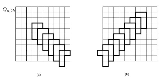
Figure 6. Diagonal minimal patterns

If $E_{\bar{\j}}$ is a translation of $R$, say $R(\bar{\j}_{1},\bar{\j}_{2})$, then $R(\bar{\j}_{1}+1,\bar{\j}_{2}-1)$ (the translation of $E_{\bar{\j}}$ by $(1,-1)$) is also part of the family $\{E_{j}\}$. Indeed if it were not so then the square $[0,2]\times[0,2]+(\bar{\j}_{1},\bar{\j}_{2})$ (i.e., the square defining the upper-left corner of $R(\bar{\j}_{1}+1,\bar{\j}_{2}-1)$) would belong to an element of the form $S(\bar{\i}_{1},\bar{\i}_{2})$. But then the square $[0,2]\times[0,1]+(\bar{\j}_{1},\bar{\j}_{2})$ would not belong to $E$, which is a contradiction. By proceeding by induction we deduce that among the sets $E_{j}$ there are all the translations of $E_{\bar{\j}}$ in direction $(1,-1)$ contained in $Q_{2k+2}(n)$; i.e., all the sets of the form $R(\bar{\j}_{1}+t,\bar{\j}_{2}-t)$, with $t\in{\mathbb{N}}$, as long as $R(\bar{\j}_{1}+t,\bar{\j}_{2}-t)\subset Q_{2k+2}(n)$ (see Fig. 6a).

Step $2$. We now prove that also the translations $R(\bar{\j}_{1}-t,\bar{\j}_{2}+t)$ with $t\in{\mathbb{N}}$ (i.e., also the translations of $E_{\bar{\j}}$ in direction $(-1,1)$) belong to the family $\{E_{j}\}$ as long as $R(\bar{\j}_{1}-t,\bar{\j}_{2}+t)\subset Q_{2k-2}(n)$. We can proceed by finite induction. It suffices to consider the case $R(\bar{\j}_{1},\bar{\j}_{2})\subset Q_{2k-4}(n)$ and prove that $R(\bar{\j}_{1}-1,\bar{\j}_{2}+1)$ belongs to the family $\{E_{j}\}$.

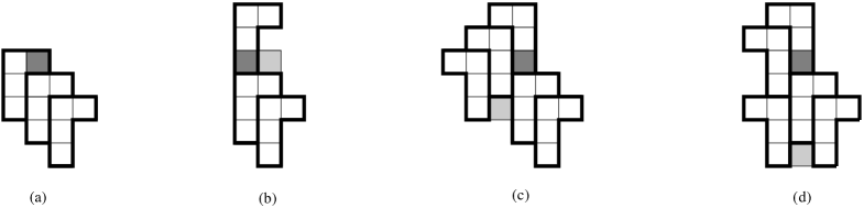
Figure 7. Necessity of upper-left translations

We suppose otherwise and argue by contradiction. Referring to Fig. 7 for a visual interpretation of the proof, we note that the square $Q=[\bar{\j}_{1},\bar{\j}_{1}+1]\times[\bar{\j}_{2}+3,\bar{\j}_{2}+4]$ (the dark gray square in Fig. 7) belongs to $E$. If it belonged to a molecule $R(\bar{\i})$ (the case in Fig. 7(b)) then this molecule should be $R(\bar{\j}_{1},\bar{\j}_{2}+3)$. In this case, the neighbouring square $[\bar{\j}_{1}+1,\bar{\j}_{1}+2]\times[\bar{\j}_{2}+3,\bar{\j}_{2}+4]$ would not belong to $E$. Since this is not the case, $Q$ must belong to some molecule $S(\bar{\i})$ belonging to $\{E_{j}\}$, which is the one pictured in Fig. 7 (c) and (d). Then also $S(\bar{\i}+(-1,-1))$ must belong to $\{E_{j}\}$ (for the same reasoning as in Step $1$). We then have two possibilities, pictured in Fig. 7(c) and (d), respectively: either $S(\bar{\i}+(-2,-2))$ belongs to $\{E_{j}\}$, in which case the light gray square in Fig. 7(c) does not belong to $E$, or $S(\bar{\i}+(-1,-4))$ belongs to $\{E_{j}\}$, in which case the light gray square in Fig. 7(d) does not belong to $E$. Note that in the latter case we reach a contradiction if the light gray square in Fig. 7(d) also belongs to $Q_{2k}(n)$. To this end we use the assumption $k>3$.

Step $3$. We can reason symmetrically if $E_{\bar{\j}}$ is a translation of $S$, say $S(\bar{\j}_{1},\bar{\j}_{2})$.

From Steps 1 and 2 we deduce that if $R(\bar{\j}_{1},\bar{\j}_{2})\subset Q_{2k}(n)$ is part of the family $\{E_{j}\}$ then all the translations $R(\bar{\j}_{1}+t,\bar{\j}_{2}-t)$ contained in $Q_{2k}(n)$ with $t\in{\mathbb{Z}}$ belong to the family $\{E_{j}\}$, and symmetrically that if $S(\bar{\j}_{1},\bar{\j}_{2})\subset Q_{2k}(n)$ is part of the family $\{E_{j}\}$ then all the translations $S(\bar{\j}_{1}+t,\bar{\j}_{2}+t)$ contained in $Q_{2k}(n)$ with $t\in{\mathbb{Z}}$ belong to the family $\{E_{j}\}$

Step $4$. Consider now a set $E_{j}$ with $E_{j}\cap Q_{2k-4}(n)\neq\mathchar 31\relax$. We may suppose again $E_{j}=R(\bar{\j})$. From the previous steps also the sets $R(\bar{\j}_{1}+t,\bar{\j}_{2}-t)$ intersecting $Q_{2k-4}(n)$ with $t\in{\mathbb{Z}}$ belong to the family $\{E_{j}\}$. Consider a unit square $Q$ in $Q_{2k-4}(n)$ neighbouring some of those $R(\bar{\j}_{1}+t,\bar{\j}_{2}-t)$. If it belonged to some $S(\bar{\i})$ belonging to the family $\{E_{j}\}$ then by the previous steps the set $S(\bar{\i}+(-1,-1))$ would belong to the family $\{E_{j}\}$ (if $Q$ lies above some $R(\bar{\j}_{1}+t,\bar{\j}_{2}-t)$) or the set $S(\bar{\i}+(1,1))$ would belong to the family $\{E_{j}\}$ (if $Q$ lies below some $R(\bar{\j}_{1}+t,\bar{\j}_{2}-t)$). In any case we would have a non-empty intersection between two elements of $\{E_{j}\}$, which is a contradiction. This implies that each such $Q$ belongs to a set $R(\bar{\i})$ of the same modulated phase of $R(\bar{\j})$. This gives that the two stripes neighboring the one of $R(\bar{\j})$ are of the same modulated phase. Proceeding by finite induction we conclude that all $E_{j}$ intersecting $Q_{2k-4}(n)$ belong to the same modulated phase. ∎

Remark 1.2.

It can be proved that the thesis of Lemma 1.1 holds with $E_{j}\cap Q_{2k{-2}}(n)\neq\mathchar 31\relax$. However the proof is more involved and we will not need such a sharp description.

From Lemma 1.1 we deduce that it is not possible to tessellate ${\mathbb{R}}^{2}$ using disjoint translations of both $R$ and $S$, or of different modulated phases of the same pattern, as stated in the following corollary.

Corollary 1.3.

Let $E=\bigcup E_{j}\in{\mathcal{A}}$ and suppose that $E={\mathbb{R}}^{2}$. Then there exists $i\in\{1,\dots,8\}$ such that $E_{j}\in{\mathcal{A}}_{i}$ for all $j$, or, equivalently, $\{E_{j}\}={\mathcal{Z}}_{i}$.

Remark 1.4 (other types of chiral molecules).

Figure 8. Other types of chiral molecules

In [15] other pairs of chiral molecules occupying four sites of a square lattice are considered. Such pairs, represented as union of squares, are pictured in Fig. 8.

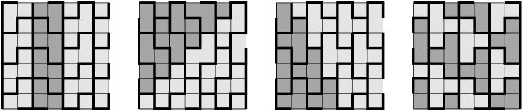
Figure 9. Configurations violating Lemma 1.1

The energy per molecule is again given by (0.1), but in this case Lemma 1.1 does not hold, as shown by the configurations in Fig. 9. As a result we do not have a parameterization of ground states that can be used to define a compact convergence as in the next section.

2. Convergence to a partition

Let $\Omega\subset{\mathbb{R}}^{2}$ be an open bounded set with Lipschitz-continuous boundary. For each $\varepsilon>0$, we define ${\mathcal{E}}^{\varepsilon}(\Omega)$ as the collection of families of essentially disjoint unions of translations of $\varepsilon R$ and $\varepsilon S$ defined as

$${\mathcal{E}}^{\varepsilon}(\Omega):=\left\{\{E^{\varepsilon}_{j}\}_{j}:\hbox{there exists }\{E_{j}\}_{j}\in{\mathcal{E}}\hbox{ such that }E^{\varepsilon}_{j}=\varepsilon E_{j}\hbox{ for all }j\hbox{, and }E^{\varepsilon}_{j}\subset\Omega\right\}.$$

We denote by ${\mathcal{A}}^{\varepsilon}(\Omega)$ as the family of sets defined as unions of families in $\mathcal{E}^{\varepsilon}(\Omega)$; i.e.,

$${\mathcal{A}}^{\varepsilon}(\Omega):=\Biggl{\{}\bigcup_{j}E_{j}:\{E_{j}\}_{j}\in{\mathcal{E}}_{\varepsilon}(\Omega)\Biggr{\}}.$$

We also define

$${\mathcal{Z}}_{i}^{\varepsilon}:=\begin{cases}\{\varepsilon R(n):n\in{\mathbb{Z}}^{2},n_{2}+n_{1}\equiv i\,\mathop{\mathrm{missing}}{mod}4\}\text{ for }i=1,\dots,4,\\ \{\varepsilon S(n):n\in{\mathbb{Z}}^{2},n_{2}-n_{1}\equiv i\,\mathop{\mathrm{missing}}{mod}4\}\text{ for }i=5,\dots,8.\end{cases}$$

Furthermore, we denote by ${\mathcal{P}}^{9}(\Omega)$ the family of ordered partitions $(A_{0},A_{1},\dots,A_{8})$ of $\Omega$ into nine sets of finite perimeter.

Definition 2.1.

We say that a sequence $\{E^{\varepsilon}_{j}\}\in{\mathcal{E}}^{\varepsilon}(\Omega)$ converges to $A\in{\mathcal{P}}^{9}(\Omega)$, and we write $\{E^{\varepsilon}_{j}\}\to A$, if

(2.1) $$|{\Omega_{i}^{\varepsilon}}\triangle{A_{i}}|\to 0\text{ as }\varepsilon\to 0,$$

where $\Omega_{i}^{\varepsilon}:=\bigcup\{E_{j}^{\varepsilon}\colon E_{j}^{\varepsilon}\in{\mathcal{Z}}_{i}^{\varepsilon}\}$ for each $i=1,\dots,8$, and $\Omega_{0}^{\varepsilon}:=\Omega\setminus\big{(}\bigcup_{i=1}^{8}\Omega_{i}^{\varepsilon}\big{)}$.

This notion of convergence is justified by the following compactness result.

Theorem 2.2 (compactness).

Assume that $\{E_{j}^{\varepsilon}\}_{j}\in{\mathcal{E}}^{\varepsilon}(\Omega)$ is such that, having set $E^{\varepsilon}=\bigcup_{j}E_{j}^{\varepsilon}$, we have

(2.2) $$C=\sup_{\varepsilon}{\mathcal{H}}^{1}\big{(}\Omega\cap\partial E^{\varepsilon}\big{)}<+\infty.$$

Then (up to relabeling) there exists a subsequence $\{E^{\varepsilon}_{j}\}$ converging to some $A\in{\mathcal{P}}^{9}(\Omega)$ in the sense of Definition 2.1.

Proof.

We use the notation $Q^{\varepsilon}_{r}(x)$ for the rescaled cube $\varepsilon Q_{r}(x)=Q_{\varepsilon r}(\varepsilon x)$.

Introduce a cover $\{Q^{\varepsilon}_{12}(n)\}_{n\in 4{\mathbb{Z}}^{2}}$ of ${\mathbb{R}}^{2}$ using squares of sides $12\varepsilon$ and center a point $\varepsilon n\in 4\varepsilon{\mathbb{Z}}^{2}$.

Set

$$I^{\varepsilon}:=\{n\in 4{\mathbb{Z}}^{2}:Q^{\varepsilon}_{12(n)}\cap\Omega\neq\mathchar 31\relax\},$$

$$\hat{I}^{\varepsilon}:=\left\{n\in I^{\varepsilon}:{\mathcal{H}}^{1}(Q^{\varepsilon}_{12}(n)\cap\partial E^{\varepsilon})\geq\varepsilon\right\}\cup\{n\in I^{\varepsilon}:Q^{\varepsilon}_{12}(n)\cap\partial\Omega\neq\mathchar 31\relax\}.$$

From (2.2) it follows that

(2.3) $$\sharp\,\hat{I}^{\varepsilon}\leq{1\over\varepsilon}\sum_{n\in\hat{I}^{\varepsilon}}{\mathcal{H}}^{1}(Q^{\varepsilon}_{12}(n)\cap\partial E^{\varepsilon})\leq{9\over\varepsilon}\sum_{m\in 4{\mathbb{Z}}^{2}}{\mathcal{H}}^{1}(\overline{Q^{\varepsilon}_{4}(m)}\cap\partial E^{\varepsilon})\leq 18\frac{C}{\varepsilon},$$

where the factor $18$ derives from the fact that a square $Q^{\varepsilon}_{4}(m)$ is contained in nine squares $Q^{\varepsilon}_{12}(n)$, and those squares have parts of the boundary in common in pairs, so that the boundary of $\partial E^{\varepsilon}$ may be accounted for twice in the last inequality. As a consequence, if we denote

$$\hat{\Omega}^{\varepsilon}=\bigcup_{n\in\hat{I}^{\varepsilon}}Q^{\varepsilon}_{12}(n),$$

then we have

(2.4) $$\bigl{|}\hat{\Omega}^{\varepsilon}\bigr{|}\leq 144\,\varepsilon^{2}\cdot 18\frac{C}{\varepsilon}=O(\varepsilon),$$

so that this set is negligible as the convergence of $\{E^{\varepsilon}_{j}\}_{j}$ is concerned.

For each $n\in I^{\varepsilon}\setminus\hat{I}^{\varepsilon}$ we apply Lemma 1.1 to $Q^{\varepsilon}_{12}(n)$ and deduce that the corresponding $Q^{\varepsilon}_{4}(n)$ satisfies: either

(2.5) $$E^{\varepsilon}\cap Q^{\varepsilon}_{4}(n)=\mathchar 31\relax,$$

or there exists $i_{\varepsilon}(n)\in\{1,\dots,8\}$ such that

(2.6) $$E_{j}^{\varepsilon}\in{\mathcal{Z}}^{\varepsilon}_{i_{\varepsilon}(n)}$$

for each $j$ such that $E_{j}^{\varepsilon}\cap Q^{\varepsilon}_{4}(n)\neq\mathchar 31\relax$. For all $i\in\{1,\dots,8\}$ we define

$$A^{\varepsilon}_{i}=\bigcup\Bigl{\{}Q^{\varepsilon}_{4}(n):n\in I^{\varepsilon}_{i}\},\hbox{ where }I^{\varepsilon}_{i}=\{n\in I^{\varepsilon}\setminus\hat{I}^{\varepsilon},i_{\varepsilon}(n)=i\}$$

and $i_{\varepsilon}(n)$ is defined in (2.6). We can estimate the length of $\partial A^{\varepsilon}_{i}$ by counting the number of the cubes of which it is composed which have a side neighboring a cube in the complement times the length $4\varepsilon$ of the corresponding interface, as

$${\mathcal{H}}^{1}(\partial A^{\varepsilon}_{i}) \leq 4\varepsilon\sharp\{n\in I^{\varepsilon}_{i}:\hbox{ there exists }n^{\prime}\in 4{\mathbb{Z}}^{2}:|n-n^{\prime}|=4\hbox{ and }n^{\prime}\not\in I^{\varepsilon}_{i}\}$$

$$\leq 4\varepsilon\sharp\{n\in I^{\varepsilon}_{i}:\hbox{ there exists }n^{\prime}\in 4{\mathbb{Z}}^{2}:|n-n^{\prime}|=4\hbox{ and }n^{\prime}\in\hat{I}^{\varepsilon}\}.$$

Indeed if $n^{\prime}\not\in\hat{I}^{\varepsilon}$ then by Lemma 1.1 we would deduce that $E^{\varepsilon}_{j}\in{\mathcal{Z}}_{i_{\varepsilon}(n^{\prime})}$ for all $j$ such that $E_{j}^{\varepsilon}\subset Q^{\varepsilon}_{8}(n^{\prime})$ and in particular for some $j$ such that $E_{j}^{\varepsilon}\subset Q^{\varepsilon}_{8}(n^{\prime})$ and $E_{j}^{\varepsilon}\cap Q^{\varepsilon}_{4}(n)\neq\mathchar 31\relax$, which then implies that $i_{\varepsilon}(n^{\prime})=i_{\varepsilon}(n)$. We can then conclude our estimate using (2.3), and deduce (since the number of possible neighbours $n^{\prime}$ is $4$) that

$$\sup_{\varepsilon}{\mathcal{H}}^{1}(\partial A^{\varepsilon}_{i})\leq\sup_{\varepsilon}16\varepsilon\,\sharp\hat{I}^{\varepsilon}\leq\sup_{\varepsilon}16\varepsilon\,{18C\over\varepsilon}<+\infty.$$

By the compactness of (bounded) sequences of equi-bounded perimeter, we deduce that there exist sets of finite perimeter $A_{1},\ldots,A_{8}$ such that (2.1) holds for $i=1,\ldots,8$, since

$$\Omega^{\varepsilon}_{i}\setminus A^{\varepsilon}_{i}\subset\hat{\Omega}_{\varepsilon},$$

which we already proved to be negligible. We finally deduce that (2.1) holds for $i=0$ by the convergence of the complement of $\Omega^{\varepsilon}_{0}$. ∎

3. Asymptotic analysis

We now describe the asymptotic behaviour of perimeter energies defined on families of molecules. We will treat in detail a fundamental case, highlighting possible extensions and variations in the sequel.

For all $\{E_{j}\}\in{\mathcal{E}}^{\varepsilon}$ we set

(3.1) $${\mathcal{F}}^{\varepsilon}(\{E_{j}\},\Omega):={\mathcal{H}}^{1}\big{(}\Omega\cap\partial E\big{)},\hbox{ where }E=\bigcup_{j}E_{j}.$$

We will prove that the asymptotic behaviour of ${\mathcal{F}}^{\varepsilon}$ as $\varepsilon\to 0$ is described by an interfacial energy defined on partitions parameterized by the nine ground states described above. To that end, we first give a definition of the limit interfacial energy density by means of an asymptotic homogenization formula.

3.1. Definition of the energy densities

Given a unit vector $\nu\in S^{1}$ and $i,j\in\{0,1,\ldots,8\}$ with $i\neq j$, we define the family $\{E_{h}^{i,j,\nu}\}$ as follows. If $i\neq 0$ then

(3.2) $$\{E_{h}^{i,0,\nu}\}=\{E\in{\mathcal{Z}}_{i}:E\cap\{x:x\cdot\nu>2\}\neq\mathchar 31\relax\},$$

(3.3) $$\{E_{h}^{0,i,\nu}\}=\{E_{h}^{i,0,-\nu}\}=\{E\in{\mathcal{Z}}_{i}:E\cap\{x:x\cdot\nu<-2\}\neq\mathchar 31\relax\};$$

i.e., $\{E_{h}^{i,0,\nu}\}$ is the family composed of elements of ${\mathcal{Z}}_{i}$ internal to the half-plane $\{x:x\cdot\nu>0\}$, and symmetrically $\{E_{h}^{0,i,\nu}\}$ is the family composed of elements of ${\mathcal{Z}}_{i}$ internal to the half-plane $\{x:x\cdot\nu<0\}$. If $i\neq 0$ and $j\neq 0$ then

(3.4) $$\{E_{h}^{i,j,\nu}\}=\{E_{h}^{i,0,\nu}\}\cup\{E_{h}^{0,j,\nu}\}.$$

In this way we have defined the family $\{E_{h}^{i,j,\nu}\}$ for all $i\neq j\in\{0,\ldots,8\}$. Note that $\{E_{h}^{j,i,\nu}\}=\{E_{h}^{i,j,-\nu}\}$.

The families defined above will allow to give a notion of boundary datum for minimum-interface problems on invading cubes. More precisely, for all $T>0$ we define the neighbourhood of $\partial Q_{T}$

(3.5) $$\delta Q_{T}:=\{x\in Q_{T}\colon\mathrm{dist}(x;\partial Q_{T})<4\}.$$

If $i\neq j$ then we set

(3.6) $$a_{i,j}(T,\nu) := \min\Big{\{}{\mathcal{F}}^{1}(\{E_{k}\},Q_{T})\colon E_{k}\in\{E_{h}^{i,j,\nu}\}\hbox{ if }E_{k}\cap\delta Q_{T}\neq\mathchar 31\relax\Big{\}},$$

where ${\mathcal{F}}^{1}$ is defined in (3.1) with $\varepsilon=1$.

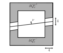
Figure 10. Sets used in the definition of boundary conditions

In order to illustrate this minimum problem, we refer to Fig. 10, and we denote by $Q^{\nu^{+}}_{T}$ and $Q^{\nu^{-}}_{T}$ the subsets $Q_{T}\cap\{x\cdot\nu>0\}$ and $Q_{T}\cap\{x\cdot\nu<0\}$ respectively. Furthermore we set

(3.7) $$\delta Q_{T}^{\nu^{+}}:=\{x\in Q^{\nu^{+}}_{T}\cap\delta Q_{r}\colon x\cdot\nu>2\},$$

(3.8) $$\delta Q_{T}^{\nu^{-}}:=\{x\in Q^{\nu^{-}}_{T}\cap\delta Q_{r}\colon x\cdot\nu<-2\},$$

The value $a_{i,j}(T,\nu)$ is the minimal length of $Q_{T}\cap\partial E$, among $E\in{\mathcal{A}}$ obtained from a family coinciding with $\{E_{h}^{i,j,\nu}\}$ on sets intersecting $\delta Q_{T}$. In particular, if $i,j\neq 0$, then the sets $\delta Q_{r}^{\nu^{+}}$ and $\delta Q_{r}^{\nu^{-}}$, represented in Fig. 10 by the shaded area, are covered by elements of $\{E_{h}\}$ in ${\mathcal{Z}}_{i}$ and ${\mathcal{Z}}_{j}$, respectively.

Definition 3.1 (energy density).

The surface energy density $f:\{0,\ldots,8\}\times\{0,\ldots,8\}\times S^{1}\to(0,+\infty)$ is defined by setting $f(i,i,\nu)=0$ and, if $i\neq j$,

(3.9) $$f(i,j,\nu):=\liminf_{T\to+\infty}\big{(}|\nu_{1}|\vee|\nu_{2}|\big{)}\frac{a_{i,j}(T,\nu)}{T},$$

where the $a_{i,j}$ are defined by minimization on $Q_{T}$ in (3.6).

The normalization factor $|\nu_{1}|\vee|\nu_{2}|$ takes into account the length of $Q_{1}\cap\{x:x\cdot\nu=0\}$.

Remark 3.2.

1. (symmetry) Note that the symmetric definition of $\{E_{h}^{i,j,\nu}\}$ gives that

$$a_{i,j}(T,\nu)=a_{j,i}(T,-\nu)$$

for all $i,j\in\{0,\ldots,8\}$ and $\nu\in S^{1}$, so that

$$f(i,j,\nu)=f(j,i,-\nu),$$

which is a necessary condition for a good definition of a surface energy.

2. (continuity) For all $i,j$ the function $f(i,j,\nu)$ is continuous on $S^{1}$. In order to check this, given $\nu$ and $\nu^{\prime}$, for fixed $T$ let $\{E^{\nu,T}_{h}\}$ be a minimizer for $a_{i,j}(T,\nu)$, and let

$$E^{\nu,T}=\bigcup\{E^{\nu,T}_{h}:|E^{\nu,T}_{h}\cap Q_{T}|\neq 0\}$$

We define $\{E^{\nu^{\prime},T}_{h}\}$ as

$$\{E^{\nu,T}_{h}:|E^{\nu,T}_{h}\cap Q_{T}|\neq 0\}\cup\{E_{h}^{i,j,\nu^{\prime}}:|E_{h}^{i,j,\nu^{\prime}}\cap E^{\nu,T}|=0\}$$

and use it to test $a_{i,j}(T+8,\nu^{\prime})$, for which it is an admissible test family. We then get

$$a_{i,j}(T+8,\nu^{\prime})\leq a_{i,j}(T,\nu)+C+CT|\nu-\nu^{\prime}|,$$

the constant $C$ estimating the contribution on $Q_{T+4}\setminus Q_{T}$, and the last term due to the mismatch of the boundary conditions close to $\partial Q_{T}$. From this inequality we deduce that $f(i,j,\nu^{\prime})-f(i,j,\nu)\leq C|\nu-\nu^{\prime}|$ and, arguing symmetrically, that

$$|f(i,j,\nu^{\prime})-f(i,j,\nu)|\leq C|\nu-\nu^{\prime}|.$$

Remark 3.3.

1. The liminf in (3.9) is actually a limit. This can be proved directly by a subadditive argument, or as a consequence of the property of convergence of minima of $\Gamma$-convergence (see Remark 3.7).

2. An alternate formula can be obtained by defining $Q^{\nu}$ as the unit square centered in $0$ and with one side orthogonal to $\nu$. We then have

(3.10) $$f(i,j,\nu):=\liminf_{T\to+\infty}{1\over T}\min\Big{\{}{\mathcal{F}}^{1}(\{E_{k}\},TQ^{\nu})\colon E_{k}\in\{E_{h}^{i,j,\nu}\}\hbox{ if }E_{k}\cap\delta TQ^{\nu}\neq\mathchar 31\relax\Big{\}},$$

where again $\delta TQ^{\nu}=\{x\in TQ^{\nu}\colon\mathrm{dist}(x;\partial Q_{T})<4\}$. Note that in this case we do not need to normalize by $|\nu_{1}|\vee|\nu_{2}|$ since the length of $Q^{\nu}\cap\{x:x\cdot\nu=0\}$ is $1$.

This formula can be again obtained as a consequence of the $\Gamma$-convergence Theorem. Conversely, a proof of Theorem 3.4 using this formula can be obtained following the same line as with the first formula, but is a little formally more complex due to the fact that the sides of $Q^{\nu}$ are not oriented in the coordinate directions. The changes in the proof can be found in the paper by Braides and Cicalese [5]. Note that usually extensions to dimensions higher than two are easier with this second formula.

3.2. $\Gamma$-limit

Let ${\mathcal{F}}_{\Omega}^{\varepsilon}$ be the functional defined for each $\{E_{j}\}\in{\mathcal{E}}^{\varepsilon}(\Omega)$ as

(3.11) $${\mathcal{F}}_{\Omega}^{\varepsilon}(\{E_{j}\})=\begin{cases}{\mathcal{F}}^{\varepsilon}(\{E_{j}\},\Omega)&\hbox{ if $\{E_{j}\}\in{\mathcal{E}}^{\varepsilon}(\Omega)$ }\cr+\infty&\hbox{ otherwise.}\end{cases}$$

We introduce the functional that assigns to every partition $A=$ $\{A_{0},\dots,A_{8}\}\in{\mathcal{P}}^{9}(\Omega)$ the real number

(3.12) $${\mathcal{F}}_{\Omega}(A):=\sum_{i=0}^{7}\sum_{j=i+1}^{8}\int_{\Omega\cap\partial A_{i}\cap\partial A_{j}}f(i,j,\nu^{i})d{\mathcal{H}}^{1}+\sum_{i=1}^{8}\int_{\partial A_{i}\cap\partial\Omega}f(i,0,\nu^{i})d{\mathcal{H}}^{1},$$

where $\nu^{i}$ is the inner normal of the set $E_{i}$ and $f$ is the interface energy defined above. We use the notation $\partial A$ to denote the reduced boundary of a set of finite perimeter $A$. Since we consider topological boundaries which coincide ${\mathcal{H}}^{1}$ almost everywhere with the corresponding reduced boundaries this notation will not cause confusion.

We use the same notation in (3.12) also when $\Omega$ is not bounded. In particular we can consider $\Omega={\mathbb{R}}^{2}$, in which case the last surface integral is not present. In that case we use the notation ${\mathcal{F}}(A)$ in the place of ${\mathcal{F}}_{{\mathbb{R}}^{2}}(A)$.

We then have the following result.

Theorem 3.4.

Let $\Omega\subset{\mathbb{R}}^{2}$ be an open bounded set with Lipschitz-continuous boundary. The sequence of functionals $\{{\mathcal{F}}^{\varepsilon}_{\Omega}\}$ defined in (3.11) $\Gamma$-converges, as $\varepsilon\to 0^{+}$, to the functional ${\mathcal{F}}_{\Omega}$ defined by (3.12), with respect to the convergence of Definition 2.1.

Remark 3.5 ($BV$-ellipticity).

As a consequence of the lower semicontinuity of ${\mathcal{F}}$ we obtain that $f$ is $BV$-elliptic [2]. In particular the extension by one-homogeneity of $f(i,j,\cdot)$ is convex for all $i,j$ and we have the subadditivity property $f(i,j,\nu)\leq f(i,k,\nu)+f(k,j,\nu)$.

Proof.

Lower bound.
We consider a partition $A=(A_{0},\ldots,A_{8})\in{\mathcal{P}}^{9}(\Omega)$ and a family $\{E^{\varepsilon}_{h}\}$ converging to $A$. We can suppose that $\liminf_{\varepsilon\to 0}{\mathcal{F}}_{\Omega}^{\varepsilon}(\{E^{\varepsilon}_{j}\})<+\infty$. We choose a subsequence $(\varepsilon_{k})$ such that

$$\lim_{k}{\mathcal{F}}_{\Omega}^{\varepsilon_{k}}(\{E^{\varepsilon_{k}}_{j}\})=\liminf_{\varepsilon\to 0}{\mathcal{F}}_{\Omega}^{\varepsilon}(\{E^{\varepsilon}_{j}\})$$

and such that the measures on $\Omega$ defined by $\mu_{\varepsilon_{k}}(B)={\mathcal{F}}_{\Omega}^{\varepsilon_{k}}(\{E^{\varepsilon_{k}}_{j}\},B)$ weakly^∗ converge to some measure $\mu$. In order not to overburden the notation we denote $\varepsilon_{k}$ simply by $\varepsilon$.

We use the blow-up method of Fonseca and Müller [11], which consists in giving a lower bound of the density of the measure $\mu$ with respect to the target measure ${\mathcal{H}}^{1}$ restricted to $\bigcup_{i}\partial A_{i}$. We refer to [6] for technical details regarding the adaptation of this method to homogenization problems.

In the present case the blow-up is performed at ${\mathcal{H}}^{1}$-almost every point $x_{0}$ in $\bigcup_{i}\partial A_{i}$. Note that this comprises also the points in $\partial\Omega$ where the inner trace of the partition at that point is not the set $A_{0}$. By a translation and slight adjustment argument (due to the fact that in general $x_{0}\not\in\varepsilon{\mathbb{Z}}^{2}$) we can simplify our notation by supposing that $x_{0}=0$. It then suffices to show that

(3.13) $$\lim_{\rho\to 0}\lim_{\varepsilon\to 0}\frac{{\mathcal{F}}^{\varepsilon}(\{E_{h}^{\varepsilon}\},Q_{\rho})}{{\mathcal{H}}^{1}(\partial A_{i}\cap\partial A_{j}\cap Q_{\rho})}\geq f(i,j,\nu),$$

supposing that $0\in\partial A_{i}\cap\partial A_{j}$ and setting $\nu=\nu^{i}(0)$.

Let $\varepsilon=\varepsilon(\rho)$ be such that $T=\rho/\varepsilon\to+\infty$ and

$$\lim_{\rho\to 0}\lim_{\varepsilon\to 0}\frac{{\mathcal{F}}^{\varepsilon}(\{E_{h}^{\varepsilon}\},Q_{\rho})}{{\mathcal{H}}^{1}(\partial A_{i}\cap\partial A_{j}\cap Q_{\rho})}=\lim_{\rho\to 0}\frac{{\mathcal{F}}^{\varepsilon(\rho)}(\{E_{h}^{\varepsilon(\rho)}\},Q_{\rho})}{{\mathcal{H}}^{1}(\partial A_{i}\cap\partial A_{j}\cap Q_{\rho})}.$$

Note that (by definition of reduced boundary) ${1\over\rho}A\cap Q_{1}$ tends to $A^{i,j,\nu}\in{\mathcal{P}}^{9}(Q_{1})$, where $A^{i,j,\nu}_{i}=Q_{1}^{\nu^{+}}$ and $A^{i,j,\nu}_{j}=Q_{1}^{\nu^{-}}$ (and therefore $A^{i,j,\nu}_{h}=\mathchar 31\relax$ for each $h\neq i,j$ and the interface $\partial A^{i,j,\nu}_{i}\cap\partial A^{i,j,\nu}_{j}$ is the segment $Q_{T}\cap\{x\cdot\nu=0\})$.

In order to prove (3.13) it is sufficient to show that

(3.14) $$\liminf_{T\to\infty}\frac{|\nu_{1}|\vee|\nu_{2}|}{T}{\mathcal{F}}^{1}(\{E^{T}_{h}\},Q_{T})\geq f(i,j,\nu),$$

with

$$\{E^{T}_{h}\}=\Bigl{\{}{1\over\varepsilon}E^{\varepsilon}_{h}\Bigr{\}}.$$

We then define $\omega^{\pm}_{T}$ as follows. We set

$$\omega^{+}_{T}=\bigcup_{h}\{E^{T}_{h}:E^{T}_{h}\in{\mathcal{Z}}_{i},\ E^{T}_{h}\subset Q_{T}^{\nu+}\}$$

if $i>0$ and

$$\omega^{+}_{T}=Q_{T}^{\nu+}\setminus\bigcup_{h}\{E^{T}_{h}\}$$

if $i=0$, and similarly

$$\omega^{-}_{T}=\bigcup_{h}\{E^{T}_{h}:E^{T}_{h}\in{\mathcal{Z}}_{j},\ E^{T}_{h}\subset Q_{T}^{\nu-}\}$$

if $j>0$ and

$$\omega^{-}_{T}=Q_{T}^{\nu-}\setminus\bigcup_{h}\{E^{T}_{h}\}$$

if $j=0$. Then

(3.15) $$|Q_{T}\setminus(\omega^{+}_{T}\cup\omega^{-}_{T})|=o(T^{2}).$$

We now show that, up to a small error, $\{E^{T}_{h}\}$ can be modified in order to fulfill the boundary conditions defined in (3.6) for each $T$. From this (3.14) follows by the definition of $a_{i,j}$.

Let $\sigma\ll 1$ and $k_{T}:=[\sigma T/12]$. We introduce a partition of the frame

$$\Bigl{\{}(x_{1},x_{2}):{T\over 2}(1-\sigma)<|x_{i}|<{T\over 2},i=1,2\Bigr{\}}=Q_{T}\setminus\overline{Q_{(1-\sigma)T}}$$

into $k_{T}$ subframes $C^{T}_{n}$ of thickness $\sigma T/2k_{T}$:

$$C^{T}_{n}:=\Big{\{}(x_{1},x_{2}):{T\over 2}\Bigl{(}1-\sigma+\frac{(n-1)\sigma}{k_{T}}\Bigr{)}<|x_{i}|<{T\over 2}\Bigl{(}1-\sigma+\frac{n\sigma}{k_{T}}\Bigr{)},i=1,2\Big{\}}$$

for $n=1,\dots,k_{T}$. Note that $\sigma T/2k_{T}\geq 6$.

From (3.15) it follows that there exists $n_{T}\in\{1,\dots,k_{T}\}$ such that

(3.16) $$|C_{n_{T}}^{T}\setminus(\omega^{+}_{T}\cup\omega^{-}_{T})|=\frac{o(T^{2})}{k_{T}}=\frac{o(T)}{\sigma}.$$

We define

$$R_{T}={T}\Bigl{(}1-\sigma+\frac{n_{T}\sigma}{k_{T}}\Bigr{)}$$

so that

$$C_{n_{T}}^{T}=Q_{R_{T}}\setminus{\overline{Q}_{R_{T}-\frac{T\sigma}{k_{T}}}}.$$

We now construct a family $\{\tilde{E}^{T}_{h}\}$ satisfying the desired boundary conditions by taking the elements of the family $\{E_{h}^{i,j,\nu}\}$ defined in (3.4) which are not contained in $Q_{R_{T}}$ union those in $\{E^{T}_{h}\}$ which do not intersect any of the former. More precisely, we define

$$E^{i,j,\nu}_{R_{T}}=\bigcup\Bigl{\{}E_{h}^{i,j,\nu}:E_{h}^{i,j,\nu}\not\subset Q_{R_{T}}\Bigr{\}}$$

and

$$\{\tilde{E}^{T}_{h}\}=\{E^{T}_{h}:|E^{i,j,\nu}_{R_{T}}\cap E^{T}_{h}|=0\}\cup\Bigl{\{}E_{h}^{i,j,\nu}:E_{h}^{i,j,\nu}\not\subset Q_{R_{T}}\Bigr{\}}.$$

Let $\tilde{E}^{T}=\bigcup_{h}\tilde{E}^{T}_{h}$. Note that, up to ${\mathcal{H}}^{1}$-negligible sets

(3.17) $$(\partial\tilde{E}^{T}\setminus\partial E^{T})\cap\overline{Q}_{R_{T}}\subset(C_{n_{T}}^{T}\setminus(\omega^{+}_{T}\cup\omega^{-}_{T})).$$

This inclusion is proved noting that points in the boundary of $\tilde{E}^{T}$ which are not in the boundary of $E^{T}$ can be subdivided into two sets: points that are in $E^{i,j,\nu}_{R_{T}}$ and those that are not. The first ones must belong to some $E^{i,j,\nu}_{h}$ with ${\mathcal{H}}^{1}\big{(}\partial E^{i,j,\nu}_{h}\cap(C_{n_{T}}^{T}\setminus(\omega^{+}_{T}\cup\omega^{-}_{T}))\big{)}\neq 0$, the second ones must be interior to $E^{T}$ but on the boundary of some $E^{T}_{h}$ with $|E^{i,j,\nu}_{R_{T}}\cap E^{T}_{h}|\neq 0$, so that in particular they also belong to $C_{n_{T}}^{T}\setminus(\omega^{+}_{T}\cup\omega^{-}_{T})$. From (3.17) and the fact that $C_{n_{T}}^{T}\setminus(\omega^{+}_{T}\cup\omega^{-}_{T})$ is composed of unit squares, using (3.16), we have

(3.18) $${\mathcal{H}}^{1}\Bigl{(}(\partial\tilde{E}^{T}\setminus\partial E^{T})\cap\overline{Q}_{R_{T}}\Bigr{)}={o(T)\over\sigma}.$$

We can estimate

$${\mathcal{H}}^{1}(Q_{T}\cap\partial\tilde{E}^{T}) = {\mathcal{H}}^{1}\Bigl{(}\overline{Q}_{R_{T}-\frac{T\sigma}{k_{T}}}\cap\partial\tilde{E}^{T}\Bigr{)}$$

$$+{\mathcal{H}}^{1}\Bigl{(}\Bigl{(}Q_{R_{T}}\setminus\overline{Q}_{R_{T}-\frac{T\sigma}{k_{T}}}\Bigr{)}\cap\partial\tilde{E}^{T}\Bigr{)}+{\mathcal{H}}^{1}((Q_{T}\setminus Q_{R_{T}})\cap\partial\tilde{E}^{T})$$

$$= {\mathcal{H}}^{1}\Bigl{(}\overline{Q}_{R_{T}-\frac{T\sigma}{k_{T}}}\cap\partial E^{T}\Bigr{)}+{\mathcal{H}}^{1}\Bigl{(}C^{T}_{n_{T}}\cap\partial\tilde{E}^{T}\cap\partial E^{T}\Bigr{)}$$

$$+{\mathcal{H}}^{1}\Bigl{(}C^{T}_{n_{T}}\cap\partial\tilde{E}^{T}\setminus\partial E^{T}\Bigr{)}+{\mathcal{H}}^{1}((Q_{T}\setminus Q_{R_{T}})\cap\partial\tilde{E}^{T})$$

$$\leq {\mathcal{H}}^{1}\Bigl{(}\overline{Q}_{R_{T}}\cap\partial E^{T}\Bigr{)}$$

$$+{\mathcal{H}}^{1}\Bigl{(}C^{T}_{n_{T}}\cap\partial\tilde{E}^{T}\setminus\partial E^{T}\Bigr{)}+{\mathcal{H}}^{1}((Q_{T}\setminus Q_{R_{T}})\cap\partial\tilde{E}^{T})$$

$$\leq {\mathcal{H}}^{1}\Bigl{(}Q_{T}\cap\partial E^{T}\Bigr{)}+{o(T)\over\sigma}+4T\sigma.$$

In terms of the functionals ${\mathcal{F}}^{1}$ this reads

$${\mathcal{F}}^{1}(\{\tilde{E}_{h}^{T}\},Q_{T})\leq{\mathcal{F}}^{1}(\{E_{h}^{T}\},Q_{T})+\frac{o(T)}{\sigma}+4\sigma T,$$

which in turn yields

$$\liminf_{T\to\infty}\frac{|\nu_{1}|\vee|\nu_{2}|}{T}{\mathcal{F}}^{1}(\{E_{h}^{T}\},Q_{T})\geq\liminf_{T\to\infty}\frac{|\nu_{1}|\vee|\nu_{2}|}{T}{\mathcal{F}}^{1}(\{\tilde{E}_{h}^{T}\},Q_{T})-4\sigma.$$

Estimate (3.14) now follows from the arbitrariness of $\sigma$ and the definition of $\tilde{E}^{T}$.

Note that if the blow-up is performed at a point in $\partial\Omega$, then $\nu$ is the inner normal to $\Omega$, $i\geq 1$ and $j=0$, which gives the boundary term in ${\mathcal{F}}_{\Omega}$.

Upper bound.
We need to show that for each $A\in{\mathcal{P}}^{9}(\Omega)$ there exists a sequence $\{E^{\varepsilon}_{j}\}\in{\mathcal{E}}^{\varepsilon}(\Omega)$ converging to $A$ and such that $\limsup_{\varepsilon}{\mathcal{F}}^{\varepsilon}(\{E^{\varepsilon}_{j}\},\Omega)\leq{\mathcal{F}}_{\Omega}(A)$. We can choose polyhedral sets $\Omega^{h}\subset\subset\Omega$ and polyhedral partitions $A^{h}$ such that $|\Omega\setminus\Omega^{h}|\to 0$, $|A^{h}_{i}\triangle A_{i}|\to 0$, ${\mathcal{H}}^{1}(\partial\Omega^{h})\to{\mathcal{H}}^{1}(\partial\Omega)$ and ${\mathcal{H}}^{1}(\partial A^{h}_{i}\cap\Omega^{h})\to{\mathcal{H}}^{1}(\partial A_{i}\cap\Omega)$, $A^{h}_{0}\supset{\mathbb{R}}^{2}\setminus\Omega$, so that ${\mathcal{F}}(A^{h})\to{\mathcal{F}}_{\Omega}(A)$ by the continuity of $f$. The existence of such $\Omega^{h}$ follows from the regularity of $\Omega$, while the construction of partitions $A^{h}$ can be derived from [7]. By an usual approximation argument ([4] Section 1.7) it thus suffices to construct recovery sequences for ${\mathcal{F}}(A)$ in the case when $\bigcup_{i=1}^{8}A_{i}\subset\subset\Omega$ and each element of the partition is a polyhedral set, provided that the approximating $\{E^{\varepsilon}_{j}\}$ belongs to ${\mathcal{E}}^{\varepsilon}(\Omega)$. In other words, it suffices to construct recovery sequences for ${\mathcal{F}}(A)$ in the case when each $A_{i}$ is a bounded polyhedral set for $i\geq 1$, provided that the approximating $E^{\varepsilon}_{j}$ belong to a small neighbourhood of $\bigcup_{i=1}^{8}A_{i}$.

Since we will reason locally, we exhibit our construction when the target partition is composed of the two half-planes $A_{l}=\{x:\nu\cdot x>0\}$ and $A_{k}=\{x:\nu\cdot x<0\}$, and $\nu$ is a rational direction; i.e., there exists $L\in{\mathbb{R}}$ such that $L\nu\in{\mathbb{Z}}^{2}$. We fix $\eta>0$ and $T=T_{\eta}$ such that

(3.20) $$\frac{|\nu_{1}|\vee|\nu_{2}|}{T}a_{l,k}(T,\nu)\leq f(l,k,\nu)+\eta$$

Up to choosing a slightly larger $T$ (at most larger $4L$ than the previous one) we can suppose that

$${T\over{|\nu_{1}|\vee|\nu_{2}|}}\nu\in 4{\mathbb{Z}}^{2}.$$

Indeed, this amounts to an additional error proportional to $4L/(T+4L)$ in (3.20), which we can include in $\eta$.

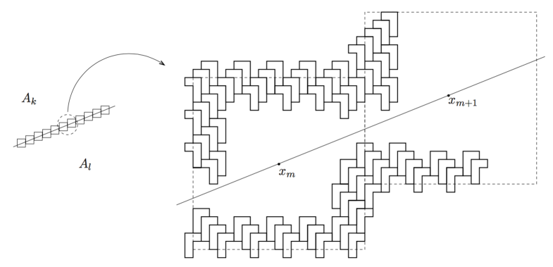
Figure 11. Construction of a recovery sequence at an interface

Let $\{E^{T}_{j}\}$ be a minimal family for $a_{l,k}(T,\nu)$. We set $\nu^{\perp}=(-\nu_{2},\nu_{1})$. We construct a sequence of molecules by covering the interfacial line $\{x:\nu\cdot x=0\}$ with the disjoint squares $E^{T}_{j}+mT{({|\nu_{1}|\vee|\nu_{2}|})^{-1}}\nu^{\perp}$ ($m\in{\mathbb{Z}}$), up to a discrete set of points, and consider the optimal family inside each such square (see Fig. 11). Since the centres of such cubes differ by a multiple of $4$ in each component, we can choose such optimal families as the translation of a single family, and match on the boundary of each cube with elements of $\{E^{l,k,\nu}_{j}\}$, which allows to extend them outside the union of the covering cubes. Note that this extension has zero energy, except for $\nu={1\over\sqrt{2}}(\pm 1,1)$, for which we may have a small contribution due to a fixed number of molecules close to the vertices of the cubes on $\{x:\nu\cdot x=0\}$; again this error will be taken care of by $\eta$.

We define $\{E^{l,k,T,\nu}_{j}\}$ as the union of all families

(3.21) $$\Bigl{\{}E^{T}_{j}+x_{m}:E^{T}_{j}\cap Q_{T}\neq\mathchar 31\relax\Bigr{\}},\qquad x_{m}=m{T\over{|\nu_{1}|\vee|\nu_{2}|}}\nu^{\perp}$$

for $m\in{\mathbb{Z}}$, and the family

(3.22) $$\Biggl{\{}E\in\{E^{l,k,\nu}_{j}\}:E\cap\bigcup_{m\in{\mathbb{Z}}}\Bigl{(}Q_{T}+m{T\over{|\nu_{1}|\vee|\nu_{2}|}}\nu^{\perp}\Bigr{)}=\mathchar 31\relax\Biggr{\}}.$$

Let now $\{E^{\varepsilon}_{j}\}$ be defined as $\{\varepsilon E_{j}\}$ with $\{E_{j}\}=\{E^{l,k,T,\nu}_{j}\}$ the family just described. Note that for all bounded open set $B$ with Lipschitz boundary such that ${\mathcal{H}}^{1}(\{\nu\cdot x=0\}\cap\partial B)=0$ we have

$$\limsup_{\varepsilon\to 0}{\mathcal{F}}(\{E^{\varepsilon}_{j}\},B)\leq\Bigl{(}f(l,k,\nu)+\eta\Bigr{)}{\mathcal{H}}^{1}(\{\nu\cdot x=0\}\cap B).$$

We now fix $A_{i}$ bounded polyhedral sets $i=1,\ldots,8$, and repeat the construction described above close to each interface. To that end, we denote

$$\bigcup_{i=1}^{8}\partial A_{i}=\{p_{m}\},$$

where $p_{m}$ are a finite number of segments with endpoints $x^{+}_{m}$ and $x^{-}_{m}$. Let $l(p_{m})$ and $k(p_{m})$ be the indices such that

$$p_{m}\subset\partial A_{l(p_{m})}\cap\partial A_{k(p_{m})}$$

and let $\nu(p_{m})$ be the inner normal to $A_{l(p_{m})}$ at $p_{m}$. In our approximation argument it is not restrictive to suppose that $\nu(p_{m})$ is a rational direction. We fix $\eta$ and $T_{m}$ such that

(3.23) $$\frac{|\nu_{1}(p_{m})|\vee|\nu_{2}(p_{m})|}{T_{m}}a_{l,k}(T_{m},\nu(p_{m}))\leq f(l(p_{m}),k(p_{m}),\nu(p_{m}))+\eta$$

and

$${T_{m}\over{|\nu_{1}(p_{m})|\vee|\nu_{2}(p_{m})|}}\nu(p_{m})\in 4{\mathbb{Z}}^{2}.$$

We choose $M$ large enough so that the distance between all points of

$$\bigcup\{p_{m}:x\hbox{ is an endpoint of }p_{m}\}\cap\partial Q_{\varepsilon M}(x)$$

is larger than $2\varepsilon(4+\sup_{m}T_{m})$.

Let $x^{m}_{\varepsilon}\in 4\varepsilon{\mathbb{Z}}^{2}$ be such that $p_{m}$ is contained in a tubular neighbourhood of the line through $x^{m}_{\varepsilon}$ and orthogonal to $\nu(p_{m})$; i.e., such that

$$p_{m}\subset\{x:(x-x^{m}_{\varepsilon})\cdot\nu(p_{m})=0\}+Q_{4\varepsilon}.$$

We denote

$$C^{\varepsilon}_{m} = \bigcup\Bigl{\{}x^{m}_{\varepsilon}+\varepsilon h{T_{m}\over{|\nu_{1}(p_{m})|\vee|\nu_{2}(p_{m})|}}\nu(p_{m})^{\perp}+Q_{\varepsilon T_{m}}:$$

$$\Bigl{(}x^{m}_{\varepsilon}+\varepsilon h{T_{m}\over{|\nu_{1}|\vee|\nu_{2}|}}\nu(p_{m})^{\perp}+Q_{\varepsilon T_{m}}\Bigr{)}\cap p_{m}\neq\mathchar 31\relax,h\in{\mathbb{Z}}\Bigr{\}}.$$

Let $\{E^{\varepsilon,m}_{j}\}$ be the elements of the family $\{\varepsilon E^{l,k,T,\nu}_{j}+x^{m}_{\varepsilon}\}$ intersecting $C^{\varepsilon}_{m}\setminus\big{(}Q_{\varepsilon M}(x^{+}_{m})\cup Q_{\varepsilon M}(x^{-}_{m})\big{)}$, where $\{E^{l,k,T,\nu}_{j}\}$ is constructed in (3.21)–(3.22) with $l=l(p_{m})$, $k=k(p_{m})$ and $\nu=\nu(p_{m})$. We then define $\{E^{\varepsilon}_{j}\}$ as the union of all $\{E^{\varepsilon,m}_{j}\}$ and of all the families

$$\Bigl{\{}\varepsilon E_{j}:E_{j}\in{\mathcal{Z}}_{i}:E_{j}\subset A_{i}\setminus\bigcup_{m}\Bigl{(}C^{\varepsilon}_{m}\cup Q_{\varepsilon M}(x^{+}_{m})\cup Q_{\varepsilon M}(x^{-}_{m})\Bigr{)}\Bigr{\}}.$$

Let $E^{\varepsilon}=\bigcup_{j}E^{\varepsilon}_{j}$. Note that the contributions due to the part of $\partial E^{\varepsilon}$ contained in each set $Q_{\varepsilon M}(x^{\pm}_{m})$ is at most of the order $\varepsilon M$. We then have that $\{E^{\varepsilon}_{j}\}$ converges to $(A_{0},\ldots,A_{8})$ and

$$\limsup_{\varepsilon\to 0}{\mathcal{F}}^{\varepsilon}(\{E^{\varepsilon}_{j}\}) \leq \sum_{m}\Bigl{(}f(l(p_{m}),k(p_{m}),\nu(p_{m}))+\eta\Bigr{)}{\mathcal{H}}^{1}(p_{m})\leq{\mathcal{F}}(A)+C\eta.$$

By the arbitrariness of $\eta$ we obtain the upper bound. ∎

Remark 3.6.

The hypothesis that $\Omega$ be bounded can be removed. In particular we can consider $\Omega={\mathbb{R}}^{2}$, in which case the term on the boundary of $\Omega$ in (3.12) disappears. The theorem can be proved in the same way, but the notion of convergence must be slightly changed by requiring that (2.1) holds when restricted to bounded sets.

On the other hand, we can define ${\mathcal{G}}_{\Omega}^{\varepsilon}$ for $\{E_{j}\}\in{\mathcal{E}}^{\varepsilon}$ as

(3.24) $${\mathcal{F}}_{\Omega}^{\varepsilon}(\{E_{j}\})=\begin{cases}{\mathcal{F}}^{\varepsilon}(\{E_{j}\},\Omega)&\hbox{ if $\{E_{j}\}\in{\mathcal{E}}^{\varepsilon}$ }\cr+\infty&\hbox{ otherwise;}\end{cases}$$

i.e., we do not require the sets ${\mathcal{E}}_{j}$ to be contained in $\Omega$. The $\Gamma$-limit is the same except for the boundary term on $\partial\Omega$, which again disappears. The liminf inequality clearly holds in the same way, while a recovery sequence can be obtained by considering first target partitions that can be extended as sets of finite perimeter in an open neighbourhood of $\Omega$, and then argue by density.

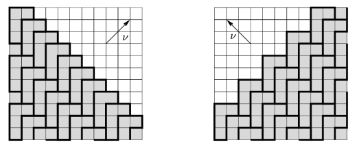
Figure 12. Optimal sets when $j=0$ in diagonal directions

3.3. Description of $f$

Computation of $f(i,0,\nu)$.  Given any $i\in\{1,\ldots,8\}$, we will explicitly compute $\varphi$, the one-positively extension of $f(i,0,\cdot)$. Since this function turns out to be symmetric, we also have $\varphi(\nu)=f(0,i,\nu)$. We treat in detail the case $i\in\{1,\ldots,4\}$. By a symmetry argument with respect to the vertical direction, we have $f(i,0,\nu)=\varphi(-\nu_{1},\nu_{2})$ for $i\in\{5,\ldots,8\}$.

We preliminarily note that a lower bound for $\varphi$ is computed by removing the constraint that the elements of $\{E_{h}\}$ be chiral molecules; i.e., taking $E_{h}$ unit squares in the lattice. The computation for the $\Gamma$-limit without the constraint is simply $\|\nu\|_{1}=|\nu_{1}|+|\nu_{2}|$ (see [1]), so that we have $\varphi(\nu)\geq|\nu_{1}|+|\nu_{2}|$.

We can check that we have equality for $\nu_{1}=\pm\nu_{2}$. Indeed, for such $\nu$ the optimal families are simply $\{E^{i,0,\nu}_{h}\}$, whose corresponding sets are those described in Fig. 12.

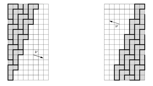
Figure 13. Optimal sets when $j=0$ in direction $\pm{1\over\sqrt{10}}(3,-1)$

Note that the value in the two direction is the same, but the ‘micro-geometry’ of optimal sets is (slightly) different. Two other values in which we have equality are with $\nu_{1}=3\nu_{2}$, with optimal families pictured in Fig. 13.

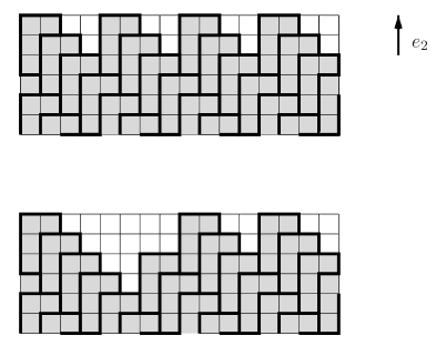
Figure 14. Optimal sets in vertical directions

We now show that $\varphi$ is a crystalline energy density (i.e., the set $\{x:\varphi(x)=1\}$ is a convex polygon, in this case an hexagon) determined by these six directions; i.e., it is linear in the cones determined by the directions. Note first that in the cones bounded by the directions ${1\over\sqrt{1}0}(3,-1)$ and ${1\over\sqrt{2}}(1,-1)$, and the directions ${1\over\sqrt{1}0}(-3,1)$ and ${1\over\sqrt{2}}(-1,1)$, $\varphi(\nu)=\|\nu\|_{1}$ since recovery sequences can be obtained by mixing those in Fig. 12 and Fig. 13.

We then note that for $\nu=e_{2}$ the optimal value is a linear combination of those in $\nu={1\over\sqrt{2}}(\pm 1,1)$, and is obtained again by $\{E^{i,0,\nu}_{h}\}$ (see Fig. 14). By the convexity of $\varphi$ this implies that $\varphi$ is linear in the cone with extreme directions ${1\over\sqrt{2}}(\pm 1,1)$. Note that, while for ${1\over\sqrt{2}}(\pm 1,1)$ the geometry of the interface is essentially unique, for $\nu=e_{1}$ this is not the case, and we may have non-periodic and arbitrary oscillations of the interface (see the lower picture in Fig. 14) The symmetric argument holds for $\nu=-e_{2}$.

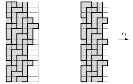
Figure 15. Optimal sets in horizontal directions

For $\nu=e_{1}$ the optimal value is a linear combination of those in the directions ${1\over\sqrt{2}}(1,1)$ and ${1\over\sqrt{1}0}(-3,1)$, which implies that $\varphi$ is linear in the cone with those extreme directions. Optimal sets are described in Fig. 15. A symmetric argument gives the same conclusion for the opposite cone.

Summarizing, $\varphi$ is a crystalline energy density determined by the values (using the one-homogeneous extension to ${\mathbb{R}}^{2}$)

$$\varphi(1,\pm 1)=\varphi(-1,\pm 1)=\varphi(\pm(3,-1))=2,$$

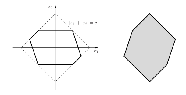
Figure 16. A level set for $f(i,0,\cdot)$ and the related Wulff shape ($1\leq i\leq 4$)

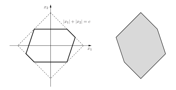
Figure 17. A level set for $f(i,0,\cdot)$ and the related Wulff shape ($5\leq i\leq 8$)

A level set $\{x:\varphi(x)=c\}$ is pictured on the left-hand side of Fig. 16. The Wulff shape related to $\varphi$ is an irregular hexagon, pictured on the right-hand side of Fig. 16. In Fig. 17 we picture the corresponding sets in the case of $f(i,0,\cdot)$ for $5\leq i\leq 8$.

Estimates.  From the symmetry of $f(i,0,,\cdot)$ and the subadditivity of $f$ we trivially have, for $i,j>0$ and $i\neq j$,

$$f(i,j,\nu)\leq f(i,0,\nu)+f(0,j,\nu)=\begin{cases}2\varphi(\nu)&\hbox{ if }i,j\leq 4\cr 2\varphi(-\nu_{1},\nu_{2})&\hbox{ if }i,j\geq 4\cr\varphi(\nu)+\varphi(-\nu_{1},\nu_{2})&\hbox{ otherwise. }\end{cases}$$

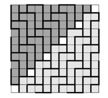
Figure 18. Test sets for $i,j\neq 0$

Note however that this may be an overestimation of $f(i,j,\nu)$: in Fig. 18 we exhibit test families that show that for $i=1$ and $j=7$ we have

$$f\Bigl{(}i,j,{1\over\sqrt{2}}(1,-1)\Bigr{)}\leq\sqrt{2}=\varphi\Bigl{(}{1\over\sqrt{2}}(1,-1)\Bigr{)}.$$

3.4. Boundary conditions

We can include in our analysis anchoring boundary conditions; i.e., we can prescribe the trace of the elements of the partition on $\partial\Omega$.

We consider a partition $\overline{A}_{0},\ldots,\overline{A}_{8}$ of ${\mathbb{R}}^{2}$ into sets of locally finite perimeter and suppose that for some $\eta>0$

$$\{x\in{\mathbb{R}}^{2}:\hbox{dist}(x,\partial\Omega)<\eta\}\cap\bigcup_{i}\partial A_{i}$$

is composed of a finite number of curves meeting $\partial\Omega$ transversally. We suppose that the families $\{\overline{E}^{\varepsilon}_{j}\}$ defined by

$$\bigcup_{i=1}^{8}\{\varepsilon E_{j}:E_{j}\in{\mathcal{Z}}_{i},\ \varepsilon E_{j}\subset\overline{A}_{i}\}$$

have equibounded energy and converge to the partition $(\overline{A}_{0},\ldots,\overline{A}_{8})$ on bounded sets of ${\mathbb{R}}^{2}$.

The family $\{\overline{E}^{\varepsilon}_{j}\}$ can be used to define boundary conditions for ${\mathcal{F}}^{\varepsilon}$, by setting

$${\mathcal{F}}^{\varepsilon}_{0}(\{E^{\varepsilon}_{j}\})=\begin{cases}{\mathcal{F}}^{\varepsilon}(\{E^{\varepsilon}_{j}\}{;\Omega})&\hbox{ if $\{E^{\varepsilon}_{j}\}\in{\mathcal{E}}^{\varepsilon}_{0}$,}\cr+\infty&\hbox{otherwise}\end{cases}$$

where ${\mathcal{E}}^{\varepsilon}_{0}$ is the collection of families in $\{E^{\varepsilon}_{j}\}\in{\mathcal{E}}^{\varepsilon}$ such that $E^{\varepsilon}_{j}\in\{\overline{E}^{\varepsilon}_{j}\}$ if $E^{\varepsilon}_{j}\cap({\mathbb{R}}^{2}\setminus\Omega_{8\varepsilon})\neq\mathchar 31\relax$, where $\Omega_{\eta}=\{x\in\Omega:\hbox{dist}(x,\partial\Omega)>\eta\}$. In particular, the sets of families $\{E^{\varepsilon}_{j}\}\in{\mathcal{E}}^{\varepsilon}_{0}$ that intersect the boundary are sets in $\{\overline{E}^{\varepsilon}_{j}\}$.

Then the family ${\mathcal{F}}^{\varepsilon}_{0}$ $\Gamma$-converges to

$${\mathcal{F}}_{0}(A)=\begin{cases}{\mathcal{F}}(A)&\hbox{if $A\in{\mathcal{P}}^{9}_{0}(\Omega,\overline{A})$}\cr+\infty&\hbox{otherwise,}\end{cases}$$

where $\overline{A}=(\overline{A}_{0},\ldots,\overline{A}_{8})$ and ${\mathcal{P}}^{9}_{0}(\Omega,\overline{A})$ is the collections of $A\in{\mathcal{P}}^{9}({\mathbb{R}}^{2})$ such that $A_{i}\setminus\Omega=\overline{A}_{i}\setminus\Omega$ for all $i$.

The proof of lower bound is immediate. As the construction of recovery sequences is concerned, given a recovery sequence for ${\mathcal{F}}(A)$ with $A\in{\mathcal{P}}^{9}_{0}(\Omega,\overline{A})$, we can modify its sets close to $\partial\Omega$ as in the proof of the lower bound in Theorem 3.4. Indeed, the proof therein deals with the case when $\Omega$ is a coordinate square centered in $0$ and $\overline{A}$ is a partition with $\{x:\nu\cdot x=0\}$ as the unique interface.

As a consequence of the fundamental theorem of $\Gamma$-convergence [4] we then have that minimum values and minimizers for ${\mathcal{F}}^{\varepsilon}_{0}$ converge to the minimum value and a minimizer of ${\mathcal{F}}_{0}$.

Remark 3.7.

We note that by its BV-ellipticity properties [2], the function $f$ satisfies

$${1\over|\nu_{1}|\vee|\nu_{2}|}f(l,k,\nu)=\min\Bigl{\{}\sum_{i<j}\int_{\overline{Q}\cap\partial A_{i}\cap\partial A_{j}}f(i,j,\nu^{i})d{\mathcal{H}}^{1}:A\in{\mathcal{P}}^{9}(l,k,\nu)\Bigr{\}}$$

where ${\mathcal{P}}^{9}(l,k,\nu)$ is the set of partitions $A$ such that $A=\overline{A}$ on ${\mathbb{R}}^{2}\setminus Q$ and $\overline{A}$ is any fixed partition such that $\overline{A}_{l}=\{x:\nu\cdot x>0\}$ and $\overline{A}_{k}=\{x:\nu\cdot x<0\}$ in an external neighbourhood of $Q$. By the previous remark this minimum can be see as the limit as $\varepsilon\to 0$ of the minima for the corresponding approximating sequence, which can be expressed in terms of the minima $a_{ij}({1\over\varepsilon},\nu)$. By renaming $T={1\over\varepsilon}$ we obtain the limit formula for $f$

(3.25) $${1\over|\nu_{1}|\vee|\nu_{2}|}f(i,j,\nu)=\lim_{T\to+\infty}{1\over T}\min\Big{\{}{\mathcal{F}}^{1}(\{E_{k}\},Q_{T})\colon E_{k}\in\{E_{h}^{i,j,\nu}\}\hbox{ if }E_{k}\cap\delta Q_{T}\neq\mathchar 31\relax\Big{\}},$$

which proves that the $\liminf$ in (3.9) is actually a limit. Similarly, we obtain the limit formula (3.10) repeating the same argument with $Q^{\nu}$ in the place of $Q$.

3.5. Alternate descriptions

From Theorem 3.4 we can derive descriptions for the limit of the energies ${\mathcal{F}}^{\varepsilon}$ with respect to other types of convergence.

We can consider the energies ${\mathcal{F}}^{\varepsilon}$ as defined on sets ${\mathcal{A}}^{\varepsilon}(\Omega)$. We define

(3.26) $${\mathcal{F}}^{\varepsilon}_{\Omega,s}(E)={\mathcal{H}}^{1}(\Omega\cap\partial E)\hbox{ if }E=\bigcup_{j}E_{j}\hbox{ and }\{E_{j}\}\in{\mathcal{E}}^{\varepsilon}(\Omega).$$

The subscript $s$ stands for “spin”. By this notation we imply that we regard a union of molecules as a constrained spin system and we do not wish to distinguish between different types of molecules. We then may consider the convergence $E^{\varepsilon}\to E$, defined as $|E^{\varepsilon}\triangle E|\to 0$ as $\varepsilon\to 0$, for which the sequence ${\mathcal{F}}^{\varepsilon}$ is equi-coercive. From Theorem 3.4 we deduce the following result.

Theorem 3.8.

Let ${\mathcal{F}}_{\Omega,s}^{\varepsilon}$ be defined by (3.26). Then the $\Gamma$-limit of ${\mathcal{F}}_{\Omega,s}^{\varepsilon}$ with respect to the convergence $E^{\varepsilon}\to E$ is defined on sets of finite perimeter $E$ by

(3.27) $${\mathcal{F}}_{\Omega,s}(E)=\inf\Biggl{\{}{\mathcal{F}}_{\Omega}(A):A=(A_{0},\ldots,A_{8})\in{\mathcal{P}}^{9}(\Omega),\bigcup_{i=1}^{8}A_{i}=E\Biggr{\}}.$$

Proof.

In order to prove the lower bound it suffices to remark that if $\sup_{\varepsilon}{\mathcal{F}}^{\varepsilon}_{\Omega,s}(E_{\varepsilon})<+\infty$ and $E_{\varepsilon}\to E$ then, up to subsequences, we can decompose $E_{\varepsilon}=\bigcup_{i=1}^{8}E^{i}_{\varepsilon}$ with $E^{i}_{\varepsilon}\to A^{i}$, so that

$$\liminf_{\varepsilon\to 0}{\mathcal{F}}^{\varepsilon}_{\Omega,s}(E_{\varepsilon})\geq{\mathcal{F}}_{\Omega}(A)\geq{\mathcal{F}}_{\Omega,s}(E).$$

In order to prove the upper bound, we may suppose that the infimum in (3.27) is achieved by some $A=(A_{0},\ldots,A_{8})$ with $\bigcup_{i=1}^{8}A_{i}=E$. We then take a recovery sequence $\{E^{\varepsilon}_{j}\}$ for ${\mathcal{F}}_{\Omega}(A)$, and a recovery sequence for ${\mathcal{F}}_{\Omega,s}(E)$ is then given by $E^{\varepsilon}=\bigcup_{j}E^{\varepsilon}_{j}$. ∎

Remark 3.9 (non-locality of the $\Gamma$-limit).

The $\Gamma$-limit ${\mathcal{F}}_{\Omega,s}(E)$ cannot be represented as an integral on $\partial E$.

To check the non locality, consider as an example the target set $E$ obtained as the intersection of the two Wulff shapes in Fig. 16 and Fig. 17. If it were local then the optimal microstructure close to an edge with normal ${1\over\sqrt{10}}(3,-1)$ should be composed of molecules in some ${\mathcal{Z}}_{i}$ with $i\in\{1,\ldots,4\}$, while the optimal microstructure close to an edge with normal ${1\over\sqrt{10}}(3,1)$ should be composed of molecules in some ${\mathcal{Z}}_{i}$ with $i\in\{5,\ldots,8\}$. This implies that the optimal $A_{1},\ldots,A_{8}$ must have at least two non-empty sets, and the value of ${\mathcal{F}}_{\Omega,s}(E)$ depends on an interface not localized on $\partial E$.

Note more in general that we can give a local lower bound by optimizing the surface energy density at each fixed value of $\nu$. Namely, if we define

$$f(x)=\min\{f(i,0,x):i\in\{1,\ldots,8\}\},$$

then a lower bound for ${\mathcal{F}}_{\Omega,s}(E)$ is given by

$${\mathcal{F}}_{\Omega,s}(E)\geq\int_{\overline{\Omega}\cap\partial E}f^{**}(\nu)d{\mathcal{H}}^{1},$$

where $\nu$ is the inner normal to $E$ and $f^{**}$ is the convex envelope of $f$ [2]. Note that this estimate derives from (3.27) by neglecting interfacial energies in ${\mathcal{F}}_{\Omega}(A)$ which are internal to $E$; i.e., those corresponding to $\partial A_{i}\cap\partial A_{j}$ with $i,j>0$. By the computations of Section 3.3 we can give an explicit description of $f^{**}$, since it is positively one homogeneous and its level set $\{x:f^{**}(x)=1\}$ is the convex envelope of the union of the two corresponding level sets for $f(1,0,\cdot)$ and $f(5,0,\cdot)$ in Fig. 16 and Fig. 17. Since for some $\nu$ (e.g., $\nu=(1,0)$) we have $f^{**}(\nu)<f(\nu)$, for such $\nu$ the optimal interface would be obtained by a surface microstructure with both $S$ and $R$ molecules, which is not possible without introducing additional surface energy corresponding to some $\partial A_{i}\cap\partial A_{j}$ with $i\in\{1,\ldots,4\}$ and $j\in\{5,\ldots,8\}$. This shows that the lower bound is not sharp for example for sets with a vertical part of the boundary.

Another possibility is to consider the two types of molecules $R$ and $S$ as parameters; i.e., rewrite the energy as

(3.28) $${\mathcal{F}}^{\varepsilon}_{\Omega,R,S}(E_{R},E_{S})={\mathcal{H}}^{1}(\Omega\cap\partial(E_{R}\cup E_{S}))$$

$$\hbox{ if }E_{R}=\bigcup\Bigl{\{}E_{j}:E_{j}\in\bigcup_{i=1}^{4}{\mathcal{Z}}^{\varepsilon}_{i}\Bigr{\}},\quad E_{S}=\bigcup\Bigl{\{}E_{j}:E_{j}\in\bigcup_{i=5}^{8}{\mathcal{Z}}^{\varepsilon}_{i}\Bigr{\}}\hbox{ and }\{E_{j}\}\in{\mathcal{E}}^{\varepsilon}(\Omega),$$

and consider the convergence $(E^{\varepsilon}_{R},E^{\varepsilon}_{S})\to(E_{R},E_{S})$ defined as the separate convergence $E^{\varepsilon}_{R}\to E_{R}$ and $E^{\varepsilon}_{S}\to E_{S}$. Note that also this convergence is compact by Theorem 2.2, since $E^{\varepsilon}_{R}=\Omega^{\varepsilon}_{1}\cup\cdots\cup\Omega^{\varepsilon}_{4}$ and $E^{\varepsilon}_{S}=\Omega^{\varepsilon}_{5}\cup\cdots\cup\Omega^{\varepsilon}_{8}$ in the notation of Definition 2.1. We then have the following result, whose proof is essentially the same as that of Theorem 3.8.

Theorem 3.10.

Let ${\mathcal{F}}_{\Omega,R,S}^{\varepsilon}$ be defined by (3.26). Then the $\Gamma$-limit of ${\mathcal{F}}_{\Omega,R,S}^{\varepsilon}$ with respect to the convergence $(E^{\varepsilon}_{R},E^{\varepsilon}_{S})\to(E_{R},E_{S})$ is defined on pairs of sets of finite perimeter $(E_{R},E_{S})$ by

(3.29) $${\mathcal{F}}_{\Omega,R,S}(E_{R},E_{S})=\inf\Biggl{\{}{\mathcal{F}}_{\Omega}(A):A=(A_{0},\ldots,A_{8}),\bigcup_{i=1}^{4}A_{i}=E_{R},\bigcup_{i=5}^{8}A_{i}=E_{S}\Biggr{\}}.$$

Remark 3.11.

We can give a lower bound of ${\mathcal{F}}_{\Omega,R,S}$ by an interfacial energy by interpreting this functional as defined on partitions of $\Omega$ into three sets of finite perimeter $(A_{0},A_{1},A_{2})$ where $A_{1}=E_{R}$, $A_{2}=E_{S}$ and $A_{0}=\Omega\setminus(E_{R}\cup E_{S})$. By Theorem 3.4 and a minimization argument we have

$${\mathcal{F}}_{\Omega,R,S}(E_{R},E_{S}) \geq \int_{\Omega\cap\partial E_{R}\cap\partial A_{S}}f_{0}^{**}(\nu^{R})d{\mathcal{H}}^{1}$$

$$+\int_{\overline{\Omega}\cap(\partial E_{R}\setminus\partial E_{S})}f_{R}(\nu^{R})d{\mathcal{H}}^{1}+\int_{\overline{\Omega}\cap(\partial E_{S}\setminus\partial E_{R})}f_{S}(\nu^{S})d{\mathcal{H}}^{1},$$

where $f_{R}(\nu)=f(1,0,\nu)$, $f_{S}(\nu)=f(5,0,\nu)$ and

$$f_{0}(\nu)=\min\{f(i,j,\nu):i\in\{1,\ldots,4\},j\in\{5,\ldots,8\}\},$$

and $\nu^{R}$ and $\nu^{S}$ are the inner normals to $E_{R}$ and $E_{S}$, respectively. Note however that the right-hand side in (3.11) may not be a lower-semicontinuous functional on partitions, and hence should be relaxed taking a BV-elliptic envelope [2]. This computation would be necessary to check if this lower bound is actually sharp so that the functional ${\mathcal{F}}_{\Omega,R,S}$ is local. Unfortunately the computation of a BV-elliptic envelope is in general an open problem, and cannot be reduced to a computation of a convex envelope as in the case of a single set of finite perimeter.

4. Generalizations and remarks

1. We can consider an inhomogeneous dependence for the surface energy. As an example, we can fix two positive constants $c_{R}$ and $c_{S}$ and consider the functionals

$${\mathcal{F}}^{\varepsilon}(\{E_{j}\};\Omega)=c_{R}{\mathcal{H}}^{1}(\Omega\cap\partial_{R}E)+c_{S}{\mathcal{H}}^{1}(\Omega\cap\partial_{S}E),$$

where $E=\bigcup_{j}E_{j}$ and

$$\partial_{R}E=\partial E\cap\partial\bigcup\Bigl{\{}E_{j}:E_{j}\in{\mathcal{Z}}_{1}\cup\cdots\cup{\mathcal{Z}}_{4}\Bigr{\}}$$

$$\partial_{S}E=\partial E\cap\partial\bigcup\Bigl{\{}E_{j}:E_{j}\in{\mathcal{Z}}_{5}\cup\cdots\cup{\mathcal{Z}}_{8}\Bigr{\}}$$

The result is the same, upon defining the surface densities using the corresponding ${\mathcal{F}}^{1}$.

Note that is this case, when computing $f(i,0,\nu)$, we might have a wetting phenomenon; i.e., the presence of a layer of a different phase at the boundary of another. This is clear if for example $c_{S}$ is sufficiently smaller than $c_{R}$ at the boundary between the phase $0$ and the phase $1$.

Figure 19. A wetting layer

In Fig. 19 we picture a configuration giving the estimate

$$f\Bigl{(}1,0,{1\over\sqrt{2}}(-1,1)\Bigr{)}\leq{3\over 2}c_{S}\sqrt{2}+{1\over 2}c_{R}\sqrt{2},$$

which is energetically convenient with respect to the one in Fig. 12 if $3c_{S}<c_{R}$.

2. In the whole analysis we can replace the surface energy by a scaled volume energy

(4.1) $${\mathcal{F}}^{\varepsilon}(\{E_{j}\};\Omega)={1\over\varepsilon}|\Omega\setminus E|.$$

Note that in this case the empty phase disappears by the definition of the energy, so that the $\Gamma$-limit is finite only if $A_{0}=\mathchar 31\relax$.

The simplest case is $\Omega={\mathbb{R}}^{2}$. In this case the proof proceeds exactly in the same way. Indeed, the argument of Lemma 1.1 is independent of energy arguments, while in the compactness Theorem 2.2 the equi-boundedness of the energy is used to obtain estimate (2.3), which follows in an even easier way under the assumption of the equiboundedness of the energies (4.1).

The surface densities are then defined by

(4.2) $$f(i,j,\nu)=(|\nu_{1}|\vee|\nu_{2}|)\lim_{T\to+\infty}{1\over T}\min\Big{\{}\Bigl{|}Q_{T}\setminus\bigcup\{E_{k}\}\Bigr{|}\colon E_{k}\in\{E_{h}^{i,j,\nu}\}\hbox{ if }E_{k}\cap\delta Q_{T}\neq\mathchar 31\relax\Big{\}},$$

since we simply have ${\mathcal{F}}^{1}(\{E_{k}\},\Omega)=|\Omega\setminus\bigcup\{E_{k}\}|$.

The case $\Omega\neq{\mathbb{R}}^{2}$ cannot be treated straightforwardly as above, since the approximation argument of $\Omega$ by polyhedral sets in the proof of the upper inequality cannot be used. We conjecture that a different boundary term on $\partial\Omega$ arises, taking into account approximations of $\Omega$ with minimal two-dimensional measure. Note that even when the approximation is not constrained to be performed with unions of molecules this may be a delicate numerical issue [14].

3. We can give a higher-order description of our system by scaling the energy as

$${\mathcal{F}}^{\varepsilon}_{1}(\{E_{j}\};\Omega)={1\over\varepsilon}{\mathcal{H}}^{1}(\Omega\cap\partial E).$$

In this case the limit is finite only at minimizers of ${\mathcal{F}}(A;\Omega)$.

(a) If $\Omega\neq{\mathbb{R}}^{2}$ then the only minimizer is given by $A_{0}=\Omega$ and $A_{i}=\mathchar 31\relax$ for $i>0$. Sequences with equi-bounded energy are $\{E^{\varepsilon}_{j}\}$ with $\sup_{\varepsilon}\sharp\{E^{\varepsilon}_{j}\}<+\infty$. We can then define the convergence $\{E^{\varepsilon}_{j}\}\to((x_{1},r_{1},s_{1}),\ldots,(x_{N},r_{N},s_{N}))$, where $x_{k}$ are the limit points of sequences in $\{E^{\varepsilon}_{j}\}$, $r_{k}$ is the number of molecules of the type $\varepsilon R(n)$ in $\{E^{\varepsilon}_{j}\}$ converging to $x_{k}$ and $s_{k}$ is the number of molecules of the type $\varepsilon S(n)$ in $\{E^{\varepsilon}_{j}\}$ converging to $x_{k}$. The $\Gamma$-limit is then defined by

$${\mathcal{F}}_{1}(\{(x_{k},r_{k},s_{k})\}_{k})=\sum_{k}\phi(r_{k},s_{k}),$$

where

$$\phi(r,s) = \min\Bigl{\{}{\mathcal{H}}^{1}(\partial E):E=\bigcup E_{j},\{E_{j}\}_{j}\hbox{ disjoint family }$$

$$\qquad\hbox{ composed of }r\hbox{ sets }R(n_{k})\hbox{ and }s\hbox{ sets }S(m_{l})\Bigr{\}}$$

(b) If $\Omega={\mathbb{R}}^{2}$ then we have the nine minimizers with $A_{i}={\mathbb{R}}^{2}$ for some $i$ and $A_{k}=\mathchar 31\relax$ for $k\neq i$. For $i=0$ we are in the same case as above. Otherwise, we can suppose that $i=1$. We can consider the convergence $\{E^{\varepsilon}_{j}\}\to((x_{1},s_{1}),\ldots,(x_{N},s_{N}))$ with $s_{k}$ defined as above. The $\Gamma$-limit is then defined by

$${\mathcal{F}}_{1}(\{(x_{k},s_{k})\})=\sum_{k}\phi(s_{k}),$$

where

$$\phi(s) = \min\Bigl{\{}{\mathcal{H}}^{1}(\partial E):E=\bigcup E_{j},\{E_{j}\}_{j}\hbox{ disjoint family composed of}$$

$$\qquad s\hbox{ sets }S(m_{l})\hbox{ and of all the }E_{j}\in{\mathcal{Z}}_{1}\hbox{ outside a compact set}\Bigr{\}}.$$

We can conjecture that the minimizers of this problem are given by an array of $s$ sets $E_{j}$ in the same ${\mathcal{Z}}_{i}$ for some $i\geq 4$ surrounded by elements in ${\mathcal{Z}}_{1}$.

4. The analysis of the functionals ${\mathcal{F}}^{\varepsilon}$ is meaningful also if only one type of molecule is taken into account. In this case we have only four modulated phases and the limit is defined on partitions into sets of finite perimeter indexed by five parameters. The proof follows in the same way, with the interfacial energies defined by using families composed only of the type of molecule considered.

It is interesting to note that this remark applies also if we take into account only one type of molecules in the pair on right-hand side of Fig. 8. Indeed, in that case there is a single pattern for the ground states with four modulated phases and Lemma 1.1 holds (while we have already remarked that it does not hold if we consider ensembles of both molecules in that pair). On the contrary, for a single type of molecules in the pair on left-hand side of Fig. 8, it is possible to construct infinitely many different structures with zero energy composed of stripes of the same two-periodic structure (see the ones in the first picture in Fig. 9) with arbitrary vertical shifts. Hence, it is not possible to reduce to a single pattern (or a finite number of patterns) for the ground states.

Acknowledgments. The subject of this paper was inspired by a MoMA Seminar by G. Contini at Sapienza University in Rome. Part of this work was elaborated in 2014 while the first two authors were visiting the Mathematical Institute in Oxford, whose kind hospitality is gratefully acknowledged.

References

- [1] R. Alicandro, A. Braides and M. Cicalese. Phase and anti-phase boundaries in binary discrete systems: a variational viewpoint. Netw. Heterog. Media 1 (2006), 85–107
- [2] L. Ambrosio and A. Braides. Functionals defined on partitions of sets of finite perimeter, II: semicontinuity, relaxation and homogenization. J. Math. Pures. Appl. 69 (1990), 307-333.
- [3] B.C. Barnes, D.W. Siderius, and L.D. Gelb. Structure, thermodynamics, and solubility in tetromino fluids. Langmuir 25 (2009), 6702–6716.
- [4] A. Braides. -convergence for Beginners. Oxford University Press, Oxford, 2002.
- [5] A. Braides and M. Cicalese. Interfaces, modulated phases and textures in lattice systems. Preprint. 2015
- [6] A. Braides, M. Maslennikov, and L. Sigalotti. Homogenization by blow-up. Applicable Anal. 87 (2008), 1341–1356.
- [7] S. Conti, A. Garroni, and A. Massaccesi. Modeling of dislocations and relaxation of functionals on 1-currents with discrete multiplicity. Calc. Var. Part. Diff. Equations 54 (2015), 1847–1874.
- [8] G. Contini, P. Gori, F. Ronci, N. Zema, S. Colonna, M. Aschi, A. Palma, S. Turchini, D. Catone, A. Cricenti, and T. Prosperi. Chirality transfer from a single chiral molecule to 2D superstructures in alaninol on the Cu(100) surface. Langmuir 27 (2011) 7410–7418
- [9] R. Fasel, M. Parschau, and K.-H. Ernst. Amplification of chirality in two-dimensional enantiomorphous lattices. Nature 439, 449–452.
- [10] S. Haq, N. Liu, V. Humblot, A.P.J. Jansen, and R. Raval. Drastic symmetry breaking in supramolecular organization of enantiomerically unbalanced monolayers at surfaces. Nature Chemistry 1 (2009), 409–414.
- [11] I. Fonseca and S. Müller. Quasi-convex Integrands and lower semicontinuity in . SIAM J. Math. Anal. 23 (1992), 1081–1098.
- [12] I. Paci. Resolution of binary enantiomeric mixtures in two dimensions. J. Phys. Chem. C 114 (2010), 19425–19432.
- [13] I. Paci, I. Szleifer, and M.A. Ratner. Chiral separation: mechanism modeling in two-dimensional systems. J. Am. Chem. Soc. 129 (2007), 3545–3555
- [14] P. Rosakis. Continuum surface energy from a lattice model. Networks and Heterogeneous Media 9 (2014), 1556–1801
- [15] P. Szabelski and A. Woszczyk. Role of molecular orientational anisotropy in the chiral resolution of enantiomers in adsorbed overlayers. Langmuir 28 (2012), 11095–11105.