Correlated fluctuations in strongly-coupled binary networks beyond equilibrium

Abstract

Randomly coupled Ising spins constitute the classical model of collective phenomena in disordered systems, with applications covering ferromagnetism, combinatorial optimization, protein folding, stock market dynamics, and social dynamics. The phase diagram of these systems is obtained in the thermodynamic limit by averaging over the quenched randomness of the couplings. However, many applications require the statistics of activity for a single realization of the possibly asymmetric couplings in finite-sized networks. Examples include reconstruction of couplings from the observed dynamics, learning in the central nervous system by correlation-sensitive synaptic plasticity, and representation of probability distributions for sampling-based inference. The systematic cumulant expansion for kinetic binary (Ising) threshold units with strong, random and asymmetric couplings presented here goes beyond mean-field theory and is applicable outside thermodynamic equilibrium; a system of approximate non-linear equations predicts average activities and pairwise covariances in quantitative agreement with full simulations down to hundreds of units. The linearized theory yields an expansion of the correlation- and response functions in collective eigenmodes, leads to an efficient algorithm solving the inverse problem, and shows that correlations are invariant under scaling of the interaction strengths.

I Introduction

Understanding collective phenomena arising from the interactions in a many-body system is the challenging subject of many-particle physics. The characterization of the emerging states typically rests on the quantification of correlations (Binney et al., 1992). Among the simplest classical models is the Ising (binary) model (Ising, 1925), or Glauber dynamics (Glauber, 1963) in its kinetic formulation. While for symmetric random couplings (Sherrington and Kirkpatrick, 1975) these systems are within the realm of equilibrium statistical mechanics (Thouless et al., 1977), the asymmetric kinetic Ising model (Hertz et al., 1986; Derrida, 1987; Crisanti and Sompolinsky, 1987), even in the stationary state, does not reach thermodynamic equilibrium. In their Markovian formulation (Kelly, 1979) these processes are studied in the field of non-equilibrium stochastic thermodynamics (for review see Seifert, 2012, chapter 6). The methods derived in these fields have proven useful in a variety of disciplines, including computer science, biology, artificial intelligence, social sciences and economics (see e.g. Mézard et al., 1987; Nishimori, 2001; Barrat et al., 2008; Castellano et al., 2009; Stein and Newman, 2013; Sornette, 2014, and references therein).

Neuronal networks of the central nervous system are prominent examples of non-equilibrium systems due to Dale’s principle (Eccles et al., 1954; Li and Dayan, 1999), which states that a neuron either excites or inhibits all its targets. The correlations between the activities of nerve cells are functionally important (Cohen and Kohn, 2011): they influence the representation of information in population signals depending on the readout in an either detrimental (Zohary et al., 1994) or beneficial (Shamir and Sompolinsky, 2001) manner, their time-dependent modulations are linked to behavior (Kilavik et al., 2009), and they determine the influence of neuronal activity on synaptic plasticity (Markram et al., 1997; Bi and Poo, 1998; Morrison et al., 2008), the biophysical substrate underlying learning. In case of binary units (Ising spins), knowledge of pairwise covariances, moreover, proves useful for sampling-based inference (reviewed in Fiser et al., 2010) as they constitute the next order in the systematic expansion of the joint probability distribution beyond independence (cf. Glauber, 1963, eq. (22)).

Dynamic mean-field theory (Sompolinsky and Zippelius, 1982; Sompolinsky et al., 1988; Aljadeff et al., 2015; Kadmon and Sompolinsky, 2015) in the $N\to\infty$ limit effectively reduces the many body problem of a network comprised of a large number of units to a single particle interacting with a self-consistently determined field, but neglects the cross-covariances of activities between units. Ginzburg and Sompolinsky (1994) introduced pairwise correlations to the description of weakly coupled systems and Renart et al. (2010) extended the analysis to strongly coupled units in the large $N$ limit. Both approaches are, however, limited to averaged pairwise correlations. Similarly, approximate master equations for binary-state dynamics on complex networks, as recently discussed in context of the pair approximation by Gleeson (2011, 2013), are restricted to global dynamics in infinite networks.

In the current work, we derive a systematic cumulant expansion yielding an analytical description of correlations between the activities of individual pairs of units, which goes beyond averaged pairwise correlations (Ginzburg and Sompolinsky, 1994; Buice et al., 2009; Renart et al., 2010) and is applicable to a single realization of an asymmetric (directed) network. The framework links the coupling structure to the emerging correlated activity and describes the first and second order statistics for single units and pairs of units in a large, but finite, network of possibly strongly interacting elements. The analytical expressions predict a distribution of pairwise correlations with a small mean but large standard deviation, as observed experimentally (Ecker et al., 2010) in neural tissue and yet not explained theoretically. Moreover, the framework can be employed to infer the couplings between the units from the observed correlated activity, also termed the inverse problem (Aertsen and Preißl, 1990; Zheng et al., 2011; Mézard and Sakellariou, 2011; Tyrcha and Hertz, 2013).

In particular, we show that already a Gaussian truncation of the presented cumulant hierarchy yields good predictions for individual mean activities and pairwise correlations. Taking into account the subset of third order cumulants that for binary variables can be expressed by lower order ones, improves the prediction significantly. This finding demonstrates that the second order statistics suffices to capture the major features of the collective dynamics arising in random binary networks, even when the coupling is strong. Our approach consistently takes into account the network-generated fluctuations in the marginal statistics of the input to each unit in a similar spirit as the seminal work by van Vreeswijk and Sompolinsky (1996). This approach exposes peculiar features of networks of binary threshold units. For a fixed number of incoming connections to each unit, mean-field theory predicts their averaged activities to be identical. We here show how distributed mean activities arise solely from the correlations emerging in the network. Units with a hard activation threshold render covariances independent of synaptic amplitudes $J$: if all incoming connections as well as the threshold of a unit are changed proportionally, the mean activity and correlations are maintained. Hence, scaling the threshold appropriately, it is impossible to increase the influence of one unit on another by larger coupling amplitudes. This finding questions the customary division into strong ($J\propto N^{-\frac{1}{2}}$) and weak coupling ($J\propto N^{-1}$) in such systems. We here show in addition that a network with hard threshold units implements the strongest possible coupling between stochastic binary units.

The independence of covariances with respect to coupling strengths implies that the latter cannot be reconstructed from the knowledge of the activity alone. However, the amplitude and slope of covariance functions at zero time lag together uniquely determine a linearized effective coupling strength between units. A linear approximation of the dynamics of fluctuations around the stationary state leads to a modified Lyapunov equation. Decomposing the fluctuations into characteristic eigenmodes of the network shows that, to linear order, the kinetic binary network is equivalent to a system of coupled Ornstein-Uhlenbeck processes (Uhlenbeck and Ornstein, 1930; Risken, 1996). The linear description further allows for the decomposition of the response to external stimulations into eigenmodes of the system.

II First and second moments of the joint probability distribution

We here consider the classical network model of stochastic binary units, and denote the activity of unit $k$ as $n_{k}(t)$ being either $0$ or $1$, where $1$ indicates activity and $0$ inactivity (see e.g. Hertz et al., 1991; Ginzburg and Sompolinsky, 1994; van Vreeswijk and Sompolinsky, 1996; Buice et al., 2009; Renart et al., 2010; Gleeson, 2011, 2013), following the notation of Buice et al. (2009). Since we may interpret a unit as representing an individual neuron, we use the terms “unit” and “neuron” interchangeably. The state of the network of $N$ such units is described by a binary vector $\mathbf{n}=(n_{1},\ldots,n_{N})\in\{0,1\}^{N}$. The model shows transitions at random points in time between the two states $0$ and $1$ controlled by transition probabilities. Using asynchronous update (Rumelhart et al., 1986), in each infinitesimal interval $[t,t+\delta t)$ each unit in the network has the probability $\frac{1}{\tau}\delta t$ to be chosen for update (Hopfield, 1982), where $\tau$ is the time constant of the dynamics. An equivalent implementation draws the time points of update independently for all units. For a particular unit, the sequence of update points has exponentially distributed intervals with mean duration $\tau$, i.e. the update times form a Poisson process with rate $\tau^{-1}$. We employ the latter implementation in the globally time-driven (Hanuschkin et al., 2010) spiking simulator NEST (Gewaltig and Diesmann, 2007), and use a discrete time resolution $\delta t=0.1\>\mathrm{ms}$ for the intervals. The stochastic update constitutes a source of noise in the system. Given the $k$-th neuron is selected for update, the probability to end in the up-state ($n_{k}=1$) is determined by the activation function $F_{k}(\mathbf{n})$ which depends on the activity $\mathbf{n}$ of all connected units. The probability to end in the down state ($n_{k}=0$) is given by $1-F_{k}(\mathbf{n})$.

The stochastic system at time $t$ is completely determined by its probability distribution $p(\mathbf{n},t)$. The time evolution of the two point distribution $p(\mathbf{n},t,\mathbf{q},s)$ (describing the probability that the system was in state $\mathbf{q}$ at time $s$ and is in state $\mathbf{n}$ at time $t$) obeys - due to the Markov property - the same master equation (see (41) in Section X.1) as $p(\mathbf{n},t)$. Using the definitions of the first moment and the equal time as well as the two time point second moments

$$\langle n_{k}(t)\rangle := \sum_{\mathbf{n}}p(\mathbf{n},t)\,n_{k}$$ (1)

$$\langle n_{k}(t)n_{l}(t)\rangle := \sum_{\mathbf{n}}p(\mathbf{n},t)\,n_{k}n_{l}$$

$$\langle n_{k}(t)n_{l}(s)\rangle := \sum_{\mathbf{n},\mathbf{q}}p(\mathbf{n},t,\mathbf{q},s)\,n_{k}q_{l},$$

one obtains a set of differential equations for the first and second moments (Ginzburg and Sompolinsky, 1994; Buice et al., 2009; Renart et al., 2010; Helias et al., 2014), which read (for completeness, in the Appendix we included their derivation in (44))

$$\tau\frac{\partial}{\partial t}\langle n_{k}(t)\rangle = -\langle n_{k}(t)\rangle+\langle F_{k}(\mathbf{n}(t))\rangle$$

$$k\neq l\qquad\tau\frac{\partial}{\partial t}\langle n_{k}(t)n_{l}(t)\rangle = -2\langle n_{k}(t)\,n_{l}(t)\rangle+\langle F_{k}(\mathbf{n}(t))\,n_{l}(t)\rangle+\langle F_{l}(\mathbf{n}(t))\,n_{k}(t)\rangle$$ (2)

$$t>s\qquad\tau\frac{\partial}{\partial t}\langle n_{k}(t)n_{l}(s)\rangle = -\langle n_{k}(t)\,n_{l}(s)\rangle+\langle F_{k}(\mathbf{n}(t))\,n_{l}(s)\rangle,$$

where the expectation value $\langle\rangle$ defined in (1) can be interpreted as an average over realizations of the random dynamics. Note that the second line does not hold for $k=l$, but becomes the first line due to $\langle n_{k}^{2}\rangle=\langle n_{k}\rangle=:m_{k}$. The third line becomes the second line for $t\to s$. These equations are identical to eqs. (3.4)-(3.7) in (Ginzburg and Sompolinsky, 1994), to eqs. (3.12) and (3.13) in (Buice et al., 2009), and to eqs. (18)-(22) in (Renart et al., 2010, Supplementary material). These previous works have so far considered the second order statistics averaged over many pairs of neurons, i.e. $\langle n_{\alpha}n_{\beta}\rangle=\frac{1}{N_{\alpha}N_{\beta}}\,\sum_{i\in\alpha\,j\in\beta}\langle n_{i}n_{j}\rangle$. These averages are closely related to the population-averaged activities $n_{\alpha}(t)=\frac{1}{N_{\alpha}}\sum_{i\in\alpha}n_{i}(t)$ and can therefore be treated by population-averaging mean-field methods. Here, we go beyond the population-averaged level and consider the second order statistics of individual pairs. Initially, we are interested in the stationary statistics of the mean activities of individual units and their zero time lag pairwise covariances $c_{kl}=\langle n_{k}(t)n_{l}(t)\rangle-\langle n_{k}(t)\rangle\langle n_{l}(t)\rangle$, which can be deduced from (2)

$$m_{k} = \langle F_{k}(\mathbf{n})\rangle$$

$$c_{kl} = \begin{cases}\frac{1}{2}\langle F_{k}(\mathbf{n})n_{l}\rangle+\frac{1}{2}\langle F_{l}(\mathbf{n})n_{k}\rangle-m_{k}m_{l}&\quad k\neq l\\ m_{k}(1-m_{k})&\quad k=l\end{cases}.$$ (3)

III Gaussian approximation

Following (van Vreeswijk and Sompolinsky, 1996; Renart et al., 2010), we now assume a particular form for the activation function and couplings between neurons given by

$$F_{k}(\mathbf{n}) = f(h_{k}(\mathbf{n}))$$ (4)

$$h_{k} = \sum_{i=1}^{N}J_{ki}n_{i},$$

where the gain function $F_{k}(\mathbf{n})=f(h_{k}(\mathbf{n}))$ depends on the state of the network only via the summed and weighted activity $h_{k}$, which is a scalar. Here $J_{ki}$ denotes the matrix of synaptic couplings from neuron $i$ to neuron $k$. For concreteness, when comparing the analytical predictions to numerical results, we choose $f(h_{k})=H\left(h_{k}-\theta\right)$, where $H(x)=1\quad\text{for }x\geq 0,\quad 0\quad\text{else}$ is the Heaviside function. Intermediate results also hold for arbitrary gain functions $f$. If the distribution of $h_{k}$ would be known, the expectation value $\langle F_{k}\rangle$ could directly be calculated.

We aim at a self-consistent equation for the first and second moments of the activity variables (2). Van Vreeswijk et al. (van Vreeswijk and Sompolinsky, 1996) and Renart et al. (2010) invoke the central limit theorem to justify the assumption that the local field $h_{k}$ typically follows a Gaussian distribution $\mathcal{N}(\mu_{k},\sigma_{k}^{2})$ with cumulants $\mu_{k}$ and $\sigma_{k}^{2}$. These cumulants are related to cumulants of the activity variables $\mathbf{n}$ via

$$\mu_{k} = \langle h_{k}\rangle=\sum_{i}J_{ki}\langle n_{i}\rangle=(\mathbf{J}\,\mathbf{m})_{i}$$ (5)

$$\sigma_{k}^{2} = \langle h_{k}^{2}\rangle-\mu_{k}^{2}=\sum_{i,j}J_{ki}J_{kj}\left(\langle n_{i}n_{j}\rangle-\langle n_{i}\rangle\langle n_{j}\rangle\right)$$

$$= \left(\mathbf{J}\,\mathbf{C}\,\mathbf{J}^{T}\right)_{kk},$$

with the covariance matrix $c_{ij}=\langle n_{i}n_{j}\rangle-\langle n_{i}\rangle\langle n_{j}\rangle$, which contains $c_{ii}=\langle n_{i}\rangle(1-\langle n_{i}\rangle)$ on the diagonal and the vector of mean activities $m_{i}=\langle n_{i}\rangle$. In the seminal work by (van Vreeswijk and Sompolinsky, 1998), the influence of the cross-covariances on the variance in the input to a neuron was neglected. Instead, only the dominant contribution, given by the variances $c_{ii}$ of the single neurons on the diagonal, were taken into account, leading to the expression $\sigma_{k}^{2}=\sum_{i}J_{ki}^{2}m_{i}(1-m_{i})$. The additional dependence of $\sigma_{k}^{2}$ on the off-diagonal elements (5) is important for the distribution of mean activities, as we will show in the following. We note that due to the marginal binary statistics of $n_{i}$ it follows that $\langle n_{i}^{2}\rangle=\langle n_{i}\rangle$, illustrating that the second moment is uniquely determined by the first moment. We will exploit this property in the subsequent sections by expressing a subset of higher order cumulants in terms of lower order ones. Using the central-limit theorem argument, as outlined above, leads to

$$m_{k}=\langle F_{k}(\mathbf{n})\rangle \simeq \int_{-\infty}^{\infty}H(x-\theta)\,\mathcal{N}(\mu_{k},\sigma_{k}^{2},x)\,dx$$

$$= \frac{1}{2}\mathrm{erfc}\left(-\frac{\mu_{k}-\theta}{\sqrt{2}\sigma_{k}}\right).$$

To enable the extension to further corrections, we aim at a more systematic calculation of expectation values containing the gain function. Using the Fourier representation $f(x)=\frac{1}{2\pi}\int_{-\infty}^{\infty}d\omega\,\hat{f}(\omega)\,\exp\left(i\omega\,x\right)$ of the gain function $f$ we obtain

$$\langle F_{k}(\mathbf{n})\rangle_{\mathbf{n}} = \frac{1}{2\pi}\int_{-\infty}^{\infty}d\omega\,\hat{f}(\omega)\left\langle\exp\left((i\omega)\sum_{j=1}^{N}J_{kj}n_{j}\right)\right\rangle_{\mathbf{n}}$$

$$= \frac{1}{2\pi}\int_{-\infty}^{\infty}d\omega\,\hat{f}(\omega)\left\langle\exp\left((i\omega)\,h_{k}(\mathbf{n})\right)\right\rangle_{\mathbf{n}},$$

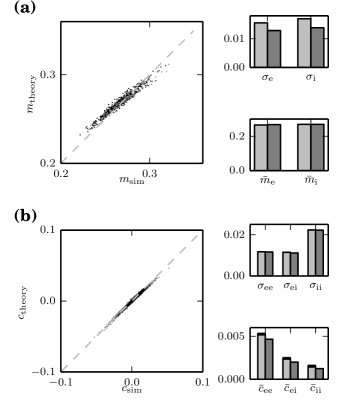
Figure 1: Consistent Gaussian approximation for the mean activity and covariance matrix in a random network of binary neurons. (a) Theoretical prediction of mean activities (15) versus simulation results (black: excitatory, gray: inhibitory). The diagonal is indicated by the dashed line. Lower inset: mean activity averaged over excitatory and inhibitory neurons (light gray: simulation, darker gray: theory). Black error bars show standard error of the mean obtained from $20$ simulations (not visible, below line width). Upper inset: width of distribution of mean activities. (b) Theoretical prediction (15) versus simulated covariance. Only cross-covariances are shown, as auto-covariances follow trivially by (3) from the mean activities. Lower inset: mean covariances averaged over excitatory-excitatory, excitatory-inhibitory and over inhibitory-inhibitory neuron pairs (light gray: simulation, darker gray: theory). Error bars show standard error of the mean obtained from $20$ simulations. Upper inset: width of the distributions of covariances. Network parameters: number of excitatory ($N_{E}=500$) and inhibitory neurons ($N_{I}=125$), threshold $\theta=-5.5$, excitatory coupling strength $J_{ij}=J=1,\,\forall j\in E$, inhibitory coupling strength $J_{ij}=-6\,J,\,\forall j\in I$, fixed in-degree homogeneous random network with connection probability $p=0.2$. Results averaged over $20$ simulations with $T=2,000,000\>\mathrm{ms}$ each. Theoretical predictions are obtained by damped fixed-point iteration (16).

where we inserted the definition of $h_{k}$ (4) in the second line. Defining the vector $\mathbf{t}$ with elements $t_{j}=i\omega J_{kj}$, the expectation value in the first line of the previous expression has the form $\langle\exp(\mathbf{t}\cdot\mathbf{n})\rangle_{\mathbf{n}}$, which is the definition the characteristic function or moment generating function

$$\varphi_{n}(\mathbf{t}) \equiv \langle e^{\mathbf{t}\cdot\mathbf{n}}\rangle_{\mathbf{n}}$$

$$= \sum_{\mathbf{n}\in\{0,1\}^{N}}p(\mathbf{n})\,e^{\mathbf{t}\cdot\mathbf{n}}$$

$$= \exp\left(\Phi_{\mathbf{n}}(\mathbf{t})\right)$$

of the joint distribution of the binary variables $p(\mathbf{n})$ (Gardiner, 1985, p. 32), which can also be expressed by the cumulant generating function $\Phi_{\mathbf{n}}(\mathbf{t})$. Note that for compactness of notation we omitted the index $j$ for $\mathbf{t}$. The Taylor expansion of $\Phi_{\mathbf{n}}(\mathbf{t})$ explicitly introduces a cumulant hierarchy showing that cumulants of activity variables $n_{j}$ at all orders contribute to $\langle F_{k}(\mathbf{n})\rangle.$ If we neglect cumulants higher than order two, thus effectively approximating the binary states as correlated Gaussian variables, we use the corresponding quadratic cumulant generating function

$$\Phi_{\mathbf{n}}(\mathbf{t}) = \sum_{i}m_{i}t_{i}+\frac{1}{2}\sum_{i,j}c_{ij}\,t_{i}t_{j}$$ (9)

and obtain

$$\langle F_{k}(\mathbf{n})\rangle_{\mathbf{n}} \simeq \frac{1}{2\pi}\int_{-\infty}^{\infty}d\omega\,\hat{f}(\omega)\,\exp\left(\sum_{i}m_{i}t_{i}+\frac{1}{2}\sum_{i,j}c_{ij}\,t_{i}t_{j}\right)$$ (10)

$$= \frac{1}{2\pi}\int_{-\infty}^{\infty}d\omega\,\hat{f}(\omega)\,\exp\left(\mu_{k}i\omega+\frac{1}{2}\sigma_{k}^{2}(i\omega)^{2}\right).$$

Here we identified the sums in the penultimate line as the mean and variance of the input field (5). On the other hand in the second line of (III) we identify the moment generating function $\varphi_{h_{k}}(i\omega)\equiv\left\langle\exp\left((i\omega)\,h_{k}(\mathbf{n})\right)\right\rangle_{\mathbf{n}}$ of the input field $h_{k}$. From (10) we obtain its corresponding cumulant generating function as $\Phi_{h_{k}}(i\omega)=\mu_{k}i\omega+\frac{1}{2}\sigma_{k}^{2}(i\omega)^{2}$. We therefore conclude that $h_{k}\sim\mathcal{N}(\mu_{k},\sigma_{k}^{2})$ follows a Gaussian distribution. The mean activity then writes

$$m_{k}=\langle F_{k}(\mathbf{n})\rangle_{\mathbf{n}} = \langle f(h_{k})\rangle_{h_{k}\sim\mathcal{N}(\mu_{k},\sigma_{k}^{2})},$$ (11)

which for $f(x)=H(x-\theta)$ is identical to (III). The procedure hence reproduces the known result for the Heaviside gain function (Van Vreeswijk and Sompolinsky, 1998; Renart et al., 2010, supplementary material, Sections 2.2, 2.3), but additionally yields a generalization for smooth gain functions $f$ that takes into account the fluctuations of the synaptic input, which is in line with the treatment in (Grytskyy et al., 2013a, eq. (27)).

More importantly, this systematic calculation reveals the assumption that is underlying the Gaussian approximation for the input field, namely that cumulants higher than order two are ignored on the level of individual neuronal activities.

To obtain an expression for the zero time lag covariance, we start from (3). We hence need to evaluate expressions of the form $\langle F_{k}(\mathbf{n})n_{l}\rangle$ which do not factorize trivially, since the value of $n_{l}$ may have an influence on neuron $k$ through the gain function $F_{k}(\mathbf{n})$. However, along the same lines as above, we can derive $\langle F_{k}(\mathbf{n})n_{l}\rangle$ using the identical approximation of $\langle\exp\left(\mathbf{n}\cdot\mathbf{t}\right)\rangle$ by first noting

$$\langle F_{k}(\mathbf{n})n_{l}\rangle = \frac{1}{2\pi}\int_{-\infty}^{\infty}d\omega\,\hat{f}(\omega)\left\langle\exp\left(i\omega\sum_{j=1}^{N}J_{kj}n_{j}\right)n_{l}\right\rangle$$

$$= \frac{1}{2\pi}\int_{-\infty}^{\infty}d\omega\,\hat{f}(\omega)\,\frac{\partial}{\partial t_{l}}\langle\exp\left(\mathbf{n}\cdot\mathbf{t}\right)\rangle.$$

Expressing again the characteristic function by the cumulant generating function (9) yields

$$\frac{\partial}{\partial t_{l}}\exp\left(\Phi_{\mathbf{n}}(\mathbf{t})\right) =\underbrace{\frac{\partial\Phi_{\mathbf{n}}(\mathbf{t})}{\partial t_{l}}}_{=m_{l}+\sum_{j}J_{kj}c_{jl}(i\omega)\text{ by \eqref{eq:quadratic_cumulant}}}\,\exp\left(\Phi_{\mathbf{n}}(\mathbf{t})\right)$$

$$=\left(m_{l}+\sum_{j}J_{kj}c_{jl}\frac{\partial}{\partial\mu_{k}}\right)\,\exp\left(\Phi_{h_{k}}(i\omega)\right),$$ (12)

where we generated the factor $i\omega$ by a derivative $\partial_{\mu_{k}}$ in the last line. With (11) this yields

$$\langle F_{k}(\mathbf{n})n_{l}\rangle = m_{l}\langle f(h_{k})\rangle_{h_{k}\sim\mathcal{N}(\mu_{k},\sigma_{k}^{2})}+S_{k}\left(JC\right)_{kl}$$ (13)

$$S_{k} = \frac{\partial}{\partial\mu_{k}}\langle f(h_{k})\rangle_{h_{k}\sim\mathcal{N}(\mu_{k},\sigma_{k}^{2})}$$

$$\stackrel{{\scriptstyle\text{i.b.p.}}}{{=}} \langle f^{\prime}(h_{k})\rangle_{h_{k}\sim\mathcal{N}(\mu_{k},\sigma_{k}^{2})},$$

where we defined the local susceptibility $S_{k}$ that determines the influence of an input to neuron $k$ onto its output at the time point of its update. For a differentiable gain function $f$ the susceptibility is equal to the slope $f^{\prime}$ averaged over the fluctuations of $h_{k}$ (compare also Grytskyy et al., 2013a, eq. (27)), which follows from integrating the second line (13) by parts (i.b.p.). For the particular choice $f(x)=H(x-\theta)$, the susceptibility has the form

$$S_{k} := \frac{1}{\sqrt{2\pi}\sigma_{k}}\,e^{-\frac{(\mu_{k}-\theta)}{2\sigma_{k}^{2}}^{2}},$$ (14)

which, by (13), is the strongest possible coupling for a given input statistics. The self-consistent set of equations for the first and second cumulants thus reads

$$m_{k} = \frac{1}{2}\mathrm{erfc}\left(-\frac{\mu_{k}-\theta}{\sqrt{2}\sigma_{k}}\right)$$

$$c_{kl} = \begin{cases}\frac{1}{2}S_{k}\left(\mathbf{JC}\right)_{kl}+\frac{1}{2}S_{l}\left(\mathbf{JC}\right)_{lk}&\quad k\neq l\\ m_{k}(1-m_{k})&\quad k=l\end{cases}.$$ (15)

To obtain the joint solution of equations (15), we use a damped fixed point iteration with the $n$-th iteration value denoted as $(m_{k}^{(n)},c_{kl}^{(n)})$, which has the form

$$m_{k}^{(n+1)} \underset{\hphantom{\text{${\scriptstyle\mbox{$k\neq l$}}$}}}{=}\rho\frac{1}{2}\mathrm{erfc}\left(-\frac{\mu_{k}^{(n)}-\theta}{\sqrt{2}\sigma_{k}^{(n)}}\right)+(1-\rho)m_{k}^{(n)}$$

$$c_{kl}^{(n+1)} \underset{\text{${\scriptstyle\mbox{$k\neq l$}}$}}{=}\rho\frac{1}{2}\left(S_{k}^{(n)}\left(\mathbf{J}\mathbf{C}^{(n)}\right)_{kl}+S_{l}^{(n)}\left(\mathbf{J}\mathbf{C}^{(n)}\right)_{lk}\right)$$

$$\underset{\hphantom{\text{${\scriptstyle\mbox{$k\neq l$}}$}}}{+}(1-\rho)c_{kl}^{(n)}$$

$$c_{kk}^{(n+1)} \underset{\text{${\scriptstyle\mbox{$k=l$}}$}}{=}m_{k}^{(n+1)}(1-m_{k}^{(n+1)}),$$ (16)

where we used the damping factor $\rho=0.7$ and determined $\mu_{k}$ and $\sigma_{k}$ via (5) in each step. The iteration continues until the summed absolute change of $m_{k}$ and $c_{kl}$ is smaller than $10^{-14}$. Figure 1 shows that the theoretical prediction yields mean activities and covariances in line with simulations of a random fixed-indegree network of excitatory and inhibitory neurons. While cross-covariances are explained with good accuracy, mean activities slightly, but systematically, deviate from simulated results: The scatter plot, showing the mean activities of individual neurons, has a slope below unity, indicating that the width of the distribution is underestimated by the theory. Moreover, we observe that the population-averaged covariances are slightly underestimated by the theory. However, in summary, the theory in the Gaussian approximation captures not only the mean and width of the covariance distribution to a large extend but also its general shape as shown in Figure 2.

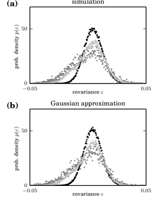
Figure 2: Distribution of covariances in the Gaussian approximation for a random network of binary neurons. (a) Distribution of cross-covariance between excitatory neurons (black), inhibitory neurons (gray) and between one inhibitory, one excitatory neuron (light gray) from simulation. (b) As (a), but showing theoretical result for the Gaussian approximation (15). Parameters as in Figure 1.

The systematic calculation presented here shows that the Gaussian assumption on the level of the individual statistics directly yields the linearized result of (Renart et al., 2010, supplementary material, Sections 2.3). Originally, the terms of the form $\langle F_{k}(\mathbf{n})n_{l}\rangle$ in (3) were obtained using relations between conditioned and unconditioned probability distributions of binary variables. After the Gaussian approximation, the resulting non-linear equation was linearized and second order terms were discussed to be small in the large $N$ limit. In contrast, the derivation here shows that the linearization is not an additional assumption, but appears naturally once the Gaussian approximation has been performed on the level of individual variables. Note also, that no additional assumption regarding the strength of the coupling is necessary.

IV Third order cumulants

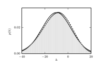
Figure 3: Distribution of the summed input. Circles show the distribution assuming uncorrelated activity of the input neurons with constant rate $m=0.2$, i.e. $p(h)=\sum_{k,l}B(pN_{E},m,k)B(pN_{I},m,l)\,\delta_{h,\>J_{E}\,k+J_{I}\,l}$ with binomial probabilities $B(N,p,k)$. Gaussian approximation $\mathcal{N}(\mu,\sigma^{2},h)$ (black) with same moments as summed binomial distribution $\mu=p\left(N_{E}J_{E}+N_{I}J_{I}\right)\,m$, $\sigma^{2}=p\left(N_{E}J_{E}^{2}+N_{I}J_{I}^{2}\right)\,m(1-m)$. Close-to-Gaussian approximation $p(h)\simeq\left(1+\frac{\kappa_{3}}{6}\,\partial_{\mu}^{3}\right)\mathcal{N}(\mu,\sigma^{2},h)$ (gray) taking into account the third cumulant $\kappa_{3}=p\left(N_{E}J_{E}^{3}+N_{I}J_{I}^{3}\right)\,(2m^{3}-3m^{2}+m)$ of $h$. Other parameters as in Figure 1.

The derivation in the previous section is systematic in the sense that all cumulants of order three and higher of the stochastic variables $\mathbf{n}$ are consistently neglected. The original idea of a mean-field description, however, seeks an approximation of the local field $h_{k}$ sensed by an individual unit $k$ rather than a truncation of the cumulants of the individual variables $\mathbf{n}$ themselves. Since the local field is by (4) a superposition of a large number of weakly correlated contributions, the distribution of $h_{k}$ will be close to Gaussian by the central limit theorem. In the path-integral formulation, commonly employed to study disordered systems, the Gaussian approximation of $h_{k}$ is equivalent to a saddle-point approximation to lowest order in the auxiliary field (see e.g. Sompolinsky and Zippelius, 1982, eq. (3.5))(Sompolinsky et al., 1988, eq. (3)). Even though one may expect the central limit theorem to be applicable to the summed input $h_{k}$, it is easy to see that for networks of several hundreds of units higher order cumulants still have an effect. This is illustrated in Figure 3, showing the distribution of the input to a neuron receiving a sum of binary, uncorrelated signals. The Gaussian approximation with the same mean and variance as the exact distribution has a peak that is slightly shifted to the left. Taking into account the third order cumulant cures the displacement of the peak. The expansion in cumulants in Section III shows how the higher order cumulants can be taken into account in the calculation of the expectation values of the gain function.

In the following we expand the distribution of $h_{k}$ up to third order cumulants. To this end we use the relationship that the $n$-th cumulant of a summed variable is the sum of $n$-th cumulants of its constituents (49). We then use the property of binary variables that $n_{k}^{K}=n_{k}$ for $K\geq 1$, which relates cumulants of order $K+L$ to cumulants of order $L+1$ in cases where neuron $k$ appears $K$ times in the cumulant (see Section X.4 for the detailed calculation). The first two cumulants of the summed input $h_{k}=\sum_{l}J_{kl}n_{l}$ to a neuron are therefore given as before by $\kappa_{1,k}=\mu_{k}$, $\kappa_{2,k}=\sigma_{k}^{2}$ (5). The third cumulant $\kappa_{3,k}$ (by defining $x_{l}=J_{kl}n_{l}$ and $y=h_{k}$ and using (49)) reads

$$\kappa_{3,k} = \sum_{ijr}J_{ki}J_{kj}J_{kr}\llangle n_{i}n_{j}n_{r}\rrangle,$$ (17)

where we use the notation $\llangle\rrangle$ to denote cumulants. For the mean activity (3) we need to evaluate the expectation value of a non-linear function applied to $h_{k}$. We follow an analogous approach as in the previous section (see Section X.3 for details) and apply (51) to $F_{k}(\mathbf{n})=H(\sum_{j}J_{kj}n_{j}-\theta)$ yielding a perturbative treatment for the effect of the third order cumulant

$$\langle F_{k}(\mathbf{n})\rangle = e^{\frac{1}{6}\kappa_{3,k}\left(\frac{\partial}{\partial\mu_{k}}\right)^{3}}\,\langle H(h_{k}-\theta)\rangle_{h_{k}\sim\mathcal{N}(\mu_{k},\sigma_{k}^{2})}.$$ (18)

To obtain a correction of the covariances, we determine the contribution of the third cumulant to the term of the form $\langle F_{k}(\mathbf{n})\,n_{l}\rangle=\langle H(h_{k}(\mathbf{n})-\theta)\,n_{l}\rangle$. We apply the general result (52) with $x_{l}=J_{kl}n_{l}$, where we need to cancel a factor $J_{kl}$ in the final result due to $n_{l}=x_{l}/J_{kl}$ to get

$$\langle F_{k}(\mathbf{n})n_{l}\rangle = \sum_{q=0}^{3}\Delta\kappa_{q,kl}\frac{1}{q!}\,\left(\frac{\partial}{\partial\mu_{k}}\right)^{q}\,\langle F_{k}(\mathbf{n})\rangle$$ (19)

with

$$\Delta\kappa_{q,kl} = \sum_{i_{1}\cdots i_{q}}J_{ki_{1}}\cdots J_{ki_{q}}\llangle n_{i_{1}}\cdots n_{i_{q}}n_{l}\rrangle,$$

where $\langle F_{k}(\mathbf{n})\rangle$ is given by (18). The form of the terms $\Delta\kappa_{q,kl}\frac{1}{q!}\,\left(\frac{\partial}{\partial\mu_{k}}\right)^{q}=\Delta\kappa_{q,kl}\frac{\partial}{\partial\kappa_{q,k}}$ shows that, for $q\geq 1$, they correspond to an infinitesimal displacement of the $q$-th cumulant $\kappa_{q,k}$ by $\Delta\kappa_{q,kl}$. These corrections come about by the presence of the variable $n_{l}$ in the expectation value, which can alternatively be understood as a conditioned expectation value $\langle F_{k}(\mathbf{n})n_{l}\rangle=m_{l}\langle F_{k}(\mathbf{n})|n_{l}=1\rangle$, where the condition $n_{l}=1$ changes the cumulants of $h_{k}$. The first two terms in the sum (19) are identical to the Gaussian approximation in (12). The difference in the approximation schemes on the level of $\mathbf{n}$ and $h_{k}$, respectively, is apparent in the term for $q=2$, which contains a correction to the second order cumulant due to the presence of $n_{l}$. This term is neglected in the Gaussian truncation of cumulants of $\mathbf{n}$ Section III. The consistent approximation of $h_{k}$ up to third order cumulants analogously requires the term for $q=3$. This correction in turn depends on the fourth order cumulant $\llangle n_{i_{1}}\cdots n_{i_{q}}n_{l}\rrangle.$

We now use the properties of binary variables that allow us to express a subset of higher cumulants by lower order ones due to the property $\langle n_{i}^{K}\rangle=\langle n_{i}\rangle$ (for all integers $K\geq 1$). The $k$-th raw moment is given by the product of all combinations of lower order cumulants (van Kampen, 1992a). For the third moment this yields

$$\langle n_{l}n_{i}n_{j}\rangle = \llangle n_{l}n_{i}n_{j}\rrangle$$

$$+ c_{li}m_{j}+c_{ij}m_{l}+c_{jl}m_{i}$$

$$+ m_{l}m_{i}m_{j}.$$

If there are at least two identical indices, we can express the corresponding third order cumulant by the two lower orders. Both cases $l=i\neq j$ and $l=i=j$ lead to the same expression (53)

$$\llangle n_{l}n_{l}n_{j}\rrangle = c_{lj}(1-2m_{l}).$$ (21)

In the latter case we get the third cumulant of a binary variable $\llangle n_{l}n_{l}n_{l}\rrangle=m_{l}-3m_{l}^{2}+2m_{l}^{3}$ which is uniquely determined by its mean. We can therefore take into account the contribution of all third order cumulants (with at least two identical indices) to the statistics of $h_{k}$. Stated differently, we calculate the third order cumulant of $h_{k}$ using (17) and neglecting all cumulants of the binary variables where all indices are different ($\llangle n_{i}n_{j}n_{l}\rrangle\simeq 0$ for $i\neq j\neq l$). A straight forward calculation (see Section X.4 eq. (54) for details) yields

$$\kappa_{3,k} \simeq \left[3(\mathbf{J}\circledast\mathbf{J})\,\mathrm{diag}(\{1-2m_{i}\})\,\mathbf{C}\mathbf{J}^{T}\right]_{kk}$$ (22)

$$- \left[2\left(\mathbf{J}\circledast\mathbf{J}\circledast\mathbf{J}\right)\,\mathrm{diag}\left(\{m_{i}-3m_{i}^{2}+2m_{i}^{3}\}\right)\right]_{k},$$

where we use the symbol $\circledast$ for the element-wise (Hadamard) product of two matrices (Cichocki et al., 2009). For the third cumulant appearing explicitly in (19) we perform a similar reduction that yields the matrix (55)

$$\Delta\kappa_{2} \simeq \mathbf{J}\circledast\mathbf{J}\,\mathrm{diag}(\{1-2m_{i}\})\mathbf{C}$$ (23)

$$+ 2\mathbf{J}\,\mathrm{diag}(\{1-2m_{i}\})\circledast(\mathbf{JC})$$

$$- 2(\mathbf{J}\circledast\mathbf{J})\,\mathrm{diag}\left(\{m_{i}-3m_{i}^{2}+2m_{i}^{3}\}\right).$$

The matrix $\Delta\kappa_{3}$ takes the form (see Section X.4 for details)

$$\Delta\kappa_{3} \simeq 3\mathbf{J}\circledast\left((\mathbf{J}\circledast\mathbf{J})\,\left\{\llangle n_{i}n_{i}n_{j}n_{j}\rrangle_{ij}\right\}\right)$$

$$+ 3(\mathbf{J}\circledast\mathbf{J})\circledast\left(\mathbf{J}\left\{\llangle n_{i}n_{j}n_{j}n_{j}\rrangle_{ij}\right\}\right)$$

$$+ (\mathbf{J}\circledast\mathbf{J}\circledast\mathbf{J})\left(\left\{\llangle n_{i}n_{i}n_{i}n_{j}\rrangle_{ij}\right\}+\mathrm{diag}(\left\{\llangle n_{i}n_{i}n_{i}n_{i}\rrangle_{i}\right\})\right),$$

where the fourth order cumulants are given by (56)-(58).

To evaluate the expression (18) for the mean activity and (19) for the covariance, we need the $n$-th derivative of the complementary error function. We use that $\frac{d}{dx}\,\frac{1}{2}\mathrm{erfc}(-x)=\frac{1}{\sqrt{\pi}}\,e^{-x^{2}}$ is a Gaussian and further that the $n$-th derivative of a Gaussian $\left(\frac{d}{dx}\right)^{n}e^{-x^{2}}=(-1)^{n}H_{n}(x)\,e^{-x^{2}}$ can be expressed in terms of the $n$-th Hermite polynomial $H_{n}$ (DLM, , 18.3 "physicists notation"). Each differentiation with respect to $\mu_{k}$ yields an additional factor $\left(\sqrt{2}\sigma_{k}\right)^{-1}$. Hence we get for $n\geq 1$

$$L_{n}(\mu_{k},\sigma_{k}) := \left(\frac{d}{d\mu_{k}}\right)^{n}\frac{1}{2}\mathrm{erfc}\left(\frac{\theta-\mu_{k}}{\sqrt{2}\sigma_{k}}\right)$$

$$= \frac{1}{\sqrt{\pi}}\,\left(\sqrt{2}\sigma_{k}\right)^{-n}\left.H_{n-1}\left(x\right)\,e^{-x^{2}}\right|_{x=\frac{\theta-\mu_{k}}{\sqrt{2}\sigma_{k}}}.$$

Using this definition and the expansion $e^{\frac{1}{6}\kappa_{3,k}\,\left(\frac{\partial}{\partial\mu_{k}}\right)^{3}}\simeq 1+\frac{1}{6}\kappa_{3,k}\,\left(\frac{\partial}{\partial\mu_{k}}\right)^{3}$, valid for $\kappa_{3,k}$ small compared to $\sigma_{k}^{3}$, we get the mean activity

$$m_{k}=\langle F_{k}(\mathbf{n})\rangle \simeq \left(1+\frac{1}{6}\kappa_{3,k}\,\left(\frac{\partial}{\partial\mu_{k}}\right)^{3}\right)\frac{1}{2}\mathrm{erfc}\left(\frac{\theta-\mu_{k}}{\sqrt{2}\sigma_{k}}\right)$$ (25)

$$= L_{0}(\mu_{k},\sigma_{k})+\frac{1}{6}\kappa_{3,k}\,L_{3}(\mu_{k},\sigma_{k}).$$

For the term appearing in the covariance we get

$$\langle F_{k}(\mathbf{n})\,n_{l}\rangle \simeq m_{l}m_{k}$$ (26)

$$+ \sum_{j=1}^{N}\left(L_{1}(\mu_{k},\sigma_{k})+\frac{1}{6}\kappa_{3,k}\,L_{4}(\mu_{k},\sigma_{k})\right)\,J_{kj}c_{jl}$$

$$+ \frac{1}{2}\left(L_{2}(\mu_{k},\sigma_{k})+\frac{1}{6}\kappa_{3,k}\,L_{5}(\mu_{k},\sigma_{k})\right)\,\Delta\kappa_{2,kl}$$

$$+ \frac{1}{6}\left(L_{3}(\mu_{k},\sigma_{k})+\frac{1}{6}\kappa_{3,k}\,L_{6}(\mu_{k},\sigma_{k})\right)\,\Delta\kappa_{3,kl}$$

$$+ o(\kappa_{3,k}^{2}).$$

The latter expression shows in particular that the correction to the mean activity reappears (as the factor $m_{k}$) in the first line, indicating that the contribution of the third cumulant to lowest order ($q=0$ in (19)) drops out of the covariance, as the term $m_{l}m_{k}$ is subtracted in (3). In a weakly correlated state of the network, the remaining terms are smaller than $m_{l}m_{k}$ as they give rise to the pairwise covariance (3). This explains why the Gaussian approximation is already fairly accurate.

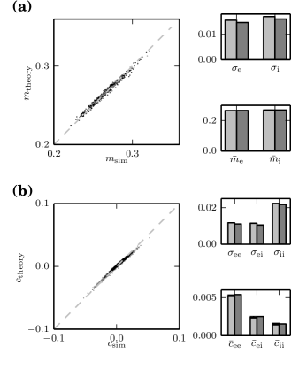
Figure 4: Approximation for covariance matrix in random network of binary neurons including third order cumulants. (a) Theoretical prediction of mean activities (25) versus simulation results (black: excitatory, gray: inhibitory). Lower inset: mean activity averaged over excitatory and inhibitory neurons (light gray: simulation, darker gray: theory). Black error bars (not visible, below line width) show standard error of the mean obtained from $20$ simulations. Upper inset: standard deviation of distribution of mean activities of excitatory ($\sigma_{e}$) and inhibitory ($\sigma_{i}$) neurons. (b) Theoretical prediction (26) versus simulated covariance (black: excitation-excitation, gray: inhibition-inhibition, light gray: excitation-inhibition). Lower inset: mean covariances averaged over excitatory-excitatory, excitatory-inhibitory and over inhibitory-inhibitory neuron pairs (light gray: simulation, darker gray: theory). Error bars show standard error of the mean obtained from $20$ simulations. Upper inset: standard deviations of the distributions of covariances. Network parameters and display as in Figure 1. Theoretical predictions obtained by damped fixed-point iteration.

Simultaneously solving (25) and (26) by a damped fixed point iteration, analogous to (16), yields an approximation of the mean activities and covariances shown in Figure 4. The deviation of the mean activities (Figure 4a) from simulation results is reduced compared to the Gaussian approximation below significance level. The width of the distributions is only slightly underestimated compared to simulations, as exhibited by the scatter plot aligned to the diagonal and the bar graph. The pairwise averaged cross-covariances (Figure 4b) are within the error of the simulated results, in contrast to the Gaussian approximation (cf. Figure 1b). A small contribution to the remaining difference in variance stems from the finite simulation time, naturally leading to a wider distribution in Figure 4b compared to the theoretical prediction. The bigger contribution presumably comes from the non-trivial third order cumulants $\llangle n_{i}n_{j}n_{k}\rrangle$, where all indices are unequal. Neglecting the non-trivial covariances shows that the variability of $\sigma_{k}$ from neuron to neuron is reduced, which in turn reduces the width of the distribution of the mean activities. For networks with fixed in-degree this even leads to a uniform mean activity across neurons, which, however, still matches the averaged mean activities from simulations indicating that averaged quantities are insensitive to variability in non-trivial higher-order cumulants (see Figure 5 in Section VI). Analogously we expect that the neglect of non-trivial third order cumulants underlies the reduced width of the covariances.

V Scale invariance of covariances

The equation for cross-covariances in (15) yields an additional insight: Assuming that mean activities and correlations were unchanged, a scaling of all incoming synapses to a neuron $k$ by some factor $\alpha>0$ amounts to a scaling of the strength of synaptic fluctuations in the same manner ($\sigma_{k}\propto\alpha$). The fixation of mean activities can be achieved for different choices of incoming synaptic amplitudes by adapting the threshold such that $\left(\mu_{k}(\{J_{kl}\})-\theta_{k}\right)/\sigma_{k}$ remains invariant (cf. (15)). A uniform rescaling of all synapses by a factor $\alpha>0$ therefore requires a change of the threshold by the same factor. The susceptibility (14) $S_{k}$ then scales as $\sigma_{k}^{-1}\propto\alpha^{-1}$. Hence the term $S_{k}J_{kl}$ appearing in the equation for covariances in (15) is invariant under this scaling. This implies that covariances are invariant with respect to the absolute value of synaptic amplitudes: The self-generated network noise causes a divisive normalization on the level of the synaptic input to each neuron. This also implies that scaling the synapses with $J\propto N^{-1}$, $J\propto N^{-\frac{1}{2}}$, or $J\propto 1$ as the network size tends to infinity all yield the same covariances, given the thresholds are adapted so that the mean activity is preserved. On the level of population-averaged covariances this has been remarked earlier (Grytskyy et al., 2013a). The independence of the network dynamics on the absolute value of the synaptic weights even holds exactly, as noted earlier (van Albada et al., 2015). The reason is the absence of a length scale of a hard threshold; the only relevant length scale is the amplitude $\sigma_{k}$ of the synaptic noise itself. Considering a single neuron $k$, the condition for the neuron to be activated is $h_{k}=\sum_{l}J_{kl}n_{l}>\theta_{k}$. Rescaling all incoming synapses as well as the threshold by the same factor $\alpha>0$ multiplies both sides of this inequality; the neuron switches at the same configuration $\mathbf{n}$ of incoming spins as in the original case. This consideration is completely in line with the work of (van Vreeswijk and Sompolinsky, 1998). The latter work found that, when increasing the number of neurons $N$, a scaling of $1/\sqrt{N}$ is required to obtain a robust asynchronous state, if the system possesses variability of the thresholds on the scale defined as unity. The width of the distribution of the thresholds induces a second length scale into the system. Invariant behavior can therefore only arise, if the synaptic noise $\sigma_{k}$ and the standard deviation of the thresholds have a constant ratio. Scaling synapses as $J\propto 1/N$ in this setting leads to vanishing temporal fluctuations of $h_{k}$ and hence spin glass freezing, whereas for $J\propto 1$ the asynchronous state persists. Fixing $J$, while increasing the number of neurons $N$, results in more inputs per neuron and thus increased temporal fluctuations, which wash out the effect of distributed thresholds.

VI Mapping of fluctuations to Ornstein-Uhlenbeck processes

We here show an alternative interpretation of the Gaussian approximation in Section III. Despite the fact that the covariances obey different equations on the diagonal $k=l$ and the off-diagonal $k\neq l$ (15), we can rewrite the equations as a single matrix equation ($\mathbf{W}=\mathbf{S}\mathbf{J}$, $\mathbf{S}=\mathrm{diag}(S_{1},\ldots,S_{N})$)

$$2\mathbf{C}-\mathbf{D} = \mathbf{WC}+(\mathbf{WC})^{T}$$ (27)

$$0 = (\mathbf{W}-\mathbf{1})\mathbf{C}+((\mathbf{W}-\mathbf{1})\mathbf{C})^{T}+\mathbf{D},$$

where $\mathbf{D}$ is a diagonal matrix with elements constrained by the condition that the diagonal entries of the covariance matrix fulfill (3)

$$c_{kk} = m_{k}(1-m_{k}).$$ (28)

We ensure this latter condition in the following way. We will first solve (27) by multiplication with the left eigenvectors $\mathbf{v}_{\alpha}$ of the connectivity, i.e. $\mathbf{v}_{\alpha}^{T}(\mathbf{W}-\mathbf{1})=\lambda_{\alpha}\mathbf{v}_{\alpha}^{T}$ (Risken, 1996, chapter 6.5). The corresponding right eigenvectors are $\mathbf{u}_{\alpha}$, which fulfill the bi-orthogonality $\mathbf{v}_{\alpha}^{T}\mathbf{u}_{\beta}=\delta_{\alpha\beta}$ and completeness $\sum_{\alpha}\mathbf{u}_{\alpha}\mathbf{v}_{\alpha}^{T}=1$ relation. With the notation $C^{\alpha\beta}:=\mathbf{v}_{\alpha}^{T}\mathbf{C}\mathbf{v}_{\beta}$ (analogously for $\mathbf{D}$) we have

$$C^{\alpha\beta} = -\frac{D^{\alpha\beta}}{\lambda_{\alpha}+\lambda_{\beta}}$$

$$\mathbf{C} = \sum_{\alpha\beta}\mathbf{u}_{\alpha}\mathbf{u}_{\beta}^{T}\,C^{\alpha\beta},$$ (29)

where the latter expression follows from the completeness relation.

The expression reveals the connection between the eigenvalues $\lambda_{\alpha}$ of the linearized coupling matrix and the fluctuations in the system. In the case of a single eigenvalue close to instability, i.e. $\Re(\lambda_{\alpha})\simeq 0$, the fluctuations in the corresponding eigendirection constitute the dominant contribution to the covariance matrix $\mathbf{C}\simeq-\mathbf{u}_{\alpha}\mathbf{u}_{\alpha}^{T}\,\frac{\mathbf{v}_{\alpha}^{T}\mathbf{D}\mathbf{v}_{\alpha}}{2\lambda_{\alpha}}$. This scenario could experimentally be detected in a principle component analysis, with the dominant principle component pointing in the direction of $\mathbf{u}_{\alpha}$.

Evaluating expression (29) on the diagonal and using $D^{\alpha\beta}=v_{\alpha}^{T}\mathbf{D}v_{\beta}=\sum_{j}v_{\alpha,j}v_{\beta,j}D_{j}$ we get

$$m_{k}(1-m_{k}) \stackrel{{\scriptstyle!}}{{=}}c_{kk}=\sum_{j}\underbrace{-\left(\sum_{\alpha\beta}\,\frac{u_{\alpha,k}v_{\alpha,j}\cdot u_{\beta,k}v_{\beta,j}}{\lambda_{\alpha}+\lambda_{\beta}}\right)}_{\equiv B_{kj}}D_{j}$$ (30)

$$\mathbf{B} =-\sum_{\alpha\beta}\frac{(\mathbf{u}_{\alpha}\mathbf{v}_{\alpha}^{T})\circledast(\mathbf{u}_{\beta}\mathbf{v}_{\beta}^{T})}{\lambda_{\alpha}+\lambda_{\beta}},$$

where the symbol $\circledast$ is to be understood as the element-wise multiplication (Hadamard product) of the two matrices in the numerator. The penultimate line is an ordinary matrix equation relating the ($N$ dimensional vector) $D_{k}$ to the ($N$ dimensional vector) $c_{kk}$. To determine $\mathbf{D}$ as $\mathbf{D}=\mathbf{B}^{-1}\mathrm{diag}(\{c_{kk}\})$ we hence need to invert the matrix $\mathbf{B}$. The covariance matrix is then obtained by (29).

The result (27) can be further interpreted as a mapping of the fluctuations from the binary dynamics to an effective system of Ornstein-Uhlenbeck processes. Given the set of coupled Ornstein-Uhlenbeck processes

$$\tau\frac{\partial x_{k}(t)}{\partial t} = -x_{k}(t)+\sum_{j}w_{kj}x_{j}(t)+\xi_{k}(t)$$ (31)

with the Gaussian white noise $\langle\mathbf{\xi}(t)\mathbf{\xi}^{T}(s)\rangle=\tau\mathbf{D}\,\delta(t-s)$, the stationary equal-time covariance matrix fulfills the same continuous Lyapunov equation (Risken, 1996, chapter 6.5) as the binary network (27). By the analogy of the continuous Lyapunov equations we see that the elements of the diagonal matrix $\mathbf{D}$ can be interpreted as the noise intensity injected into each neuron. The modified Lyapunov method (30) determines this intensity such that the variance of each continuous variable $x_{k}$ agrees to that of the corresponding binary variabe $n_{k}$ given by (28) that, in turn, is fixed by the mean activity (15).

It is important to note that $\mathbf{W}$ and $\mathbf{D}$ in (27) and (31) themselves depend on the covariances $\mathbf{C}$ via the susceptibility $\mathbf{S}$. This leads to (29) remaining an implicit equation for $\mathbf{C}$ that needs to be solved iteratively. However, by neglecting the contribution of cross-covariances in (5), $\mathbf{W}$ and $\mathbf{D}$ become independent of $\mathbf{C}$, rendering (27) a linear equation for the covariances and the above projection method an efficient algorithm to compute $\mathbf{C}$. This linear approximation consequently fails to predict the distribution of mean activities for networks with fixed indegree, as shown in Figure 5a. Nevertheless, the width of the distribution of the covariances shown in Figure 5b is only slightly underestimated, showing that the distribution of mean activities contributes only marginally to the distribution of covariances.

The viability of the linear approximation for the covariances shows that fluctuations in the binary model are practically equivalent to those in linear Ornstein-Uhlenbeck processes. This equivalence has been reported earlier for effective equations of the population-averaged pairwise correlations (Grytskyy et al., 2013b). The latter work used the approximate result $c_{kk}\simeq\frac{D_{k}}{2}$, which ignores the effect of the covariances onto the auto-covariances in (27), i.e. assuming that $(\mathbf{WC})_{kk}$ is smaller than $c_{kk}$ itself and hence neglecting the right hand side of (27) when determining the diagonal elements $c_{kk}$. In the absence of self-connections this amounts to neglecting the off-diagonal cross-covariances in $\mathbf{C}$. For weakly correlated network states this is a good approximation. However, in the present network setting it slightly overestimates the population-averages of the covariances as well as the width of their distribution (data not shown).

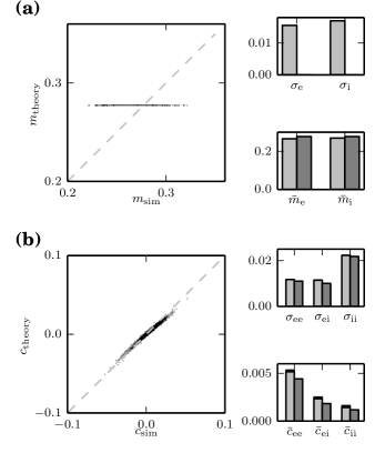
Figure 5: Modified Lyapunov method. Solution of the individual pairwise covariances by the projection method applied to the continuous Lyapunov equation in comparison to simulation results. (a) Mean activities predicted by the approximation that neglects cross-correlations (black: excitatory, gray: inhibitory). Lower inset: mean activity averaged over excitatory and inhibitory neurons (light gray: simulation, darker gray: theory). Black error bars show the standard error of the mean obtained from $20$ simulations (barely visible, approximately at line width). Upper inset: width of distribution of mean activities. (b) Theoretical distribution of covariances (29) with $\mathbf{D}$ chosen according to (30) (same approximation as in (a) for $\mathbf{m}$ and $\mathbf{S}$, i.e. neglect of cross-correlations in the input to each neuron). Lower inset: mean covariances averaged over excitatory-excitatory, excitatory-inhibitory and over inhibitory-inhibitory neuron pairs (light gray: simulation, darker gray: theory). Error bars show the standard error of the mean obtained from $20$ simulations. Upper inset: width of the distributions of covariances. Other parameters and display as in Figure 1.

VII Response of the network to external stimuli

To study how the recurrent network processes an externally applied signal, we take into account an additional external input to each neuron $k$, denoted as $h_{k,\mathrm{ext.}}(t)$, such that $h_{k}(t)=\sum_{j}J_{kj}n_{j}(t)+h_{k,\mathrm{ext.}}(t)$. We start from the differential equation (2) for the mean activities

$$\tau\frac{\partial}{\partial t}\langle n_{k}(t)\rangle =-\langle n_{k}(t)\rangle+\langle F_{k}(\mathbf{n}(t),h_{k,\mathrm{ext.}}(t))\rangle,$$

with

$$F_{k}(\mathbf{n}(t),h_{k,\mathrm{ext.}}(t)) = H\left(\sum_{j}J_{kj}n_{j}(t)+h_{k,\mathrm{ext.}}(t)-\theta\right).$$

As in the case without external input, the expectation value $\langle F_{k}(\mathbf{n}(t),h_{k,\mathrm{ext.}}(t))\rangle$ can be treated in the Gaussian approximation. Subtracting the stationary activity state $\delta n_{k}(t)=n_{k}(t)-\langle n_{k}\rangle$ we get after linearization

$$\tau\frac{\partial}{\partial t}\langle\delta n_{k}(t)\rangle = -\langle\delta n_{k}(t)\rangle+S_{k}\left(\sum_{j}J_{kj}\langle\delta n_{j}(t)\rangle+h_{k,\mathrm{ext.}}(t)\right)$$

$$= \sum_{j}(w_{kj}-\delta_{kj})\langle\delta n_{j}(t)\rangle+\underbrace{S_{k}\,h_{k,\mathrm{ext.}}(t)}_{=:y_{k}(t)},$$

where $w_{kj}=S_{k}J_{kj}$ is the effective connectivity as defined in Section VI and $S_{k}$ is the susceptibility (14). Hence the equation of motion for the perturbation in matrix notation reads

$$\tau\frac{\partial}{\partial t}\langle\delta\mathbf{n}(t)\rangle = (\mathbf{W}-\mathbf{1})\langle\delta\mathbf{n}(t)\rangle+\mathbf{y}(t).$$ (32)

In order to excite the system into the direction of one eigenmode of the effective connectivity $\mathbf{W}$, we choose the following stimulus vector

$$\mathbf{h}_{\mathrm{ext.}}^{\alpha}(t) := a\,\tilde{\mathbf{u}}_{\alpha}\,f(t),\>\mbox{with}\>\tilde{\mathbf{u}}_{\alpha}=\frac{\mathbf{S}^{-1}\Re(\mathbf{u}_{\alpha})}{\|\mathbf{S}^{-1}\Re(\mathbf{u}_{\alpha})\|},$$ (33)

where $\mathbf{S}:=\mathrm{diag}(\{S_{k}\})$ is the diagonal matrix containing the susceptibilities and $\mathbf{u}_{\alpha}$ the right-sided eigenvector of $\mathbf{W}-\mathbf{1}$ as defined in Section VI. The strength of the stimulus is regulated by the parameter $a$ and its temporal profile determined by $f(t)$. The parameter $a$ allows us to control the amplitude of the stimulation in comparison to the strength of the synaptic noise received by each unit. For the linear approximation to hold, this amplitude must be chosen such that the input to each unit is in the linear part of the expectation value of the gain function and can hence be approximated by the slope (14). Stimulating into the direction of the real part of the eigenvectors ensures that a complex mode is excited in combination with its complex conjugate, which is necessary since the activity in the network is real-valued. Here, $\tilde{\mathbf{u}}_{\alpha}$ is constructed such that it is normalized and compensates for the multiplication of the external input with the diagonal susceptibility matrix. We measure the deflection of the activity into the direction of the eigenmode by defining $\langle\delta n^{\alpha}(t)\rangle:=\tilde{\mathbf{v}}_{\alpha}^{T}\langle\delta\mathbf{n}(t)\rangle$ as the projection of the activity vector onto the $\alpha$-th eigenmode of the connectivity matrix $\mathbf{W}$ ($y^{\alpha}$ defined analogously), where we choose $\tilde{\mathbf{v}}_{\alpha}^{T}$ such that $\tilde{\mathbf{v}}_{\alpha}^{T}\mathbf{S}\tilde{\mathbf{u}}_{\beta}=\delta_{\alpha\beta}$, i.e.

$$\mathbf{\tilde{\mathbf{v}}}_{\alpha} :=k\|\mathbf{S}^{-1}\Re(\mathbf{u}_{\alpha})\|\Re(\mathbf{v}_{\alpha}),\>\mbox{with}\>k= \begin{cases}1&\quad\text{if }\Im(\lambda_{\alpha})=0\\ 2&\quad\text{if }\Im(\lambda_{\alpha})\neq 0\end{cases}$$

with $\mathbf{v}_{\alpha}$ being the left eigenvectors of $\mathbf{W}-\mathbf{1}$ as defined in Section VI.

The time evolution of the perturbation $\langle\delta n^{\alpha}(t)\rangle$ is obtained by solving (32) projected onto $\mathbf{v}_{\alpha}$ and $\mathbf{v}_{\alpha}^{*}$, and subsequently adding the results. Hence, for any stimulus $f(t)$ (inserted into (32) as $\mathbf{y}(t)=\mathbf{S}\mathbf{h}_{\mathrm{ext.}}^{\alpha}(t)$) the perturbation obeys the convolution equation

$$\langle\delta n^{\alpha}\rangle(t) = a\,\frac{1}{\tau}\,\frac{1}{2}\,\left[\left(e^{\lambda_{\alpha}\frac{\circ}{\tau}}+e^{\lambda_{\alpha}^{\ast}\frac{\circ}{\tau}}\right)\ast f\right](t).$$ (34)

We here consider an incoming DC-input starting at time $t_{0}=0$ and stopping at $t=T$, i.e. we choose $f(t)=H(t)-H(t-T)$. The time course of the perturbation is then given by

$$\langle\delta n^{\alpha}\rangle(t)=a\begin{cases}\Re\Big{(}\lambda_{\alpha}^{-1}(1-e^{\lambda_{\alpha}\frac{t}{\tau}})\Big{)}&\quad\text{if }t\leq T\\ \Re\Big{(}\lambda_{\alpha}^{-1}(e^{\lambda_{\alpha}\frac{t-T}{\tau}}-e^{\lambda_{\alpha}\frac{t}{\tau}})\Big{)}&\quad\text{if }t>T\end{cases}.$$ (35)

Figure 6 shows the response of the network activity projected onto one eigenmode to the DC-stimulus in the direction of the same eigenmode. Choosing three stimulus directions associated with three representative eigenvalues from the full eigenvalue cloud of the network (Figure 6a), we demonstrate that the time course of fast (large negative eigenvalue), slowly (eigenvalue close to zero), as well as oscillatory (complex eigenvalue) decaying modes is captured by the linear approximation. This shows how the response of the network depends on the spatial structure of the stimulation. To lowest order, the transformation performed by the network is hence a spatio-temporal filtering of the input, where the responses with slowest decay correspond to the excitation of eigenmodes closest to instability.

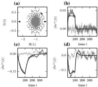
Figure 6: Linear responses to DC-stimuli. Responses (normalized by the number of units $N$) to a DC-stimulus (duration $T=100\>\mathrm{ms}$) in the direction of one eigenmode (dark gray), the background activity (light gray) measured in simulation and the analytical prediction of the response curve ((35), black) obtained from linear response theory. (a) Eigenvalues $\lambda_{\alpha}$ of the matrix $\mathbf{W}-\mathbf{1}$. The eigenvalues associated with the modes that are stimulated are depicted by black dots. (b) Stimulation in the direction of the fastest decaying eigenmode $\lambda=-2.24$, with a stimulus size $a=50$. (c) Stimulation in the direction of the slowest decaying eigenmode $\lambda=-0.26$, with a stimulus size $a=-30$. (d) Stimulation in the direction of an eigenmode decaying slowly and oscillatory $\lambda=-0.52+0.43i$, with a stimulus size $a=-60$. Responses averaged over $500$ repetitions. Other parameters as in Figure 1.

VIII Reconstruction of connectivity

In the current section we investigate the inverse problem, i.e. in how far the connectivity $J_{kl}$ of the network can be inferred from the observed activity. The time-lagged cross-covariance function in a network of Ornstein-Uhlenbeck processes (for $t>s$) fulfills the differential equation (Risken, 1996, chapter 6.5)

$$q_{kl}:=\tau\frac{\partial}{\partial t}c_{kl}(t,s) +c_{kl}(t,s)\stackrel{{\scriptstyle\text{${\scriptstyle\mbox{$t>s$}}$}}}{{=}} \sum_{j}w_{kj}c_{jl}(t,s).$$ (36)

This means we can uniquely reconstruct the connectivity $w_{kl}$ from the knowledge of the two matrices, the covariance and its slope at time lag zero as

$$\mathbf{W} = \mathbf{Q}\mathbf{C}^{-1}$$ (37)

$$= \mathbf{1}+\tau\frac{\partial}{\partial t}\left.\mathbf{C}(t,s)\right|_{t=s}\mathbf{C}^{-1}.$$

For an Ornstein-Uhlenbeck process, obeying (27) and (36), the reconstruction of the connectivity $w_{kl}$ is exact, as shown in Figure 8b.

We will now demonstrate that a similar relationship approximately also holds in binary networks. For $t>s$, the time-lagged cross-covariance function $c_{kl}(t,s)=\langle n_{k}(t)n_{l}(s)\rangle-\langle n_{k}(t)\rangle\langle n_{l}(t)\rangle$ for the binary network fulfills (45)

$$q_{kl}(t,s) := \tau\frac{\partial}{\partial t}c_{kl}(t,s)+c_{kl}(t,s)$$ (38)

$$\stackrel{{\scriptstyle\text{${\scriptstyle\mbox{$t>s$}}$}}}{{=}} \langle F_{k}(\mathbf{n}(t))\,n_{l}(s)\rangle-\langle n_{k}(t)\rangle\langle n_{l}(s)\rangle.$$

An example of an auto- and cross-covariance function together with the slope at zero time lag is shown in Figure 7.

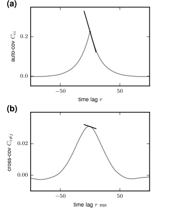
Figure 7: Auto- and cross covariance functions. Example of an auto- (a) and cross-covariance function (b) in the network described in Figure 1. The respective slopes of the functions at time lag $0+$ are indicated by the black tangent lines.

In the limit of vanishing time lag the form of $q_{kl}=\lim_{t\to s}q_{kl}(t,s)=\langle F_{k}(\mathbf{n}(t))\,n_{l}(t)\rangle-\langle n_{k}(t)\rangle\langle n_{l}(t)\rangle$ shows that $q_{kl}$ measures the direct influence of fluctuations of neuron $l$ on the gain function of neuron $k$. In the Gaussian approximation (see Section III) we get for $k\neq l$

$$q_{kl} = \sum_{j}S_{k}J_{kj}c_{jl}.$$ (39)

For $k=l$, however, we have to evaluate $\langle H(h_{k}(\mathbf{n}(t)-\theta)\,n_{k}(t)\rangle$ on the right hand side. Since the term $n_{k}$ appears in the expectation value, the statistics of $h_{k}$ is effectively conditioned on the state $n_{k}=1$. Since the transitions of neuron $k$ directly depend on the value of $h_{k}$, this conditioning violates the close-to Gaussian approximation of $h_{k}|n_{k}=1$. An approximate treatment on the diagonal is possible under the assumption that the auto-covariance function of $h_{k}$ is dominated by contributions of the auto-covariances of the binary variables $n$, yielding a non-linear differential equation for the temporal shape of the auto-covariance function (van Vreeswijk and Sompolinsky, 1998, eq. (5.17)). Approximating the temporal profile of the auto-covariance function $a(s):=\langle H(h_{k}(t+s)-\theta)\,H(h_{k}(t)-\theta)\rangle\simeq\langle m\rangle+\langle m\rangle(1-\langle m_{k}\rangle)\,e^{-\frac{|s|}{\tau}}$, which has the right asymptotic behaviors ($a(0)=m_{k}$ and $a(s\to\infty)=m_{k}^{2}$) and assumes fluctuations to be correlated on the time scale $\tau$ of the update, leads to the approximate value $\langle H(h_{k}(t)-\theta)\,n_{k}(t)\rangle\simeq\frac{1}{2}m_{k}(1-m_{k})$ (by using van Vreeswijk and Sompolinsky, 1998, eq. (A.10)). The corresponding approximation of the slope following from the former approximation with (38) is shown in Figure 8a. However, the resulting expression for the slope at zero time lag cannot be written in the form (39). Therefore, we assume that (39) also holds on the diagonal, although the resulting predicted slopes have a slight negative bias compared to simulation results.

Given the two covariance matrices entering (38), as well as the average activities $m_{i}$ for each neuron, we can derive a procedure for reconstructing the connectivity $J_{kl}/\sigma_{k}$. The mean and variance of the input to a neuron are determined by (5). Inverting the relation (III) as $y(m_{k}):=\frac{\mu_{k}-\theta}{\sqrt{2}\sigma_{k}}=-\mathrm{erfc}^{-1}(2m_{k})$ allows us to determine the susceptibility (14) as $S\left(m_{k},\sigma_{k}\right)=\frac{1}{\sqrt{2\pi}\sigma_{k}}\,e^{-y(m_{k})^{2}}$. Hence we obtain an expression for the ratio of the incoming synaptic weight and the total synaptic noise of neuron $k$

$$\frac{J_{kl}}{\sigma_{k}}= \sqrt{2\pi}w_{kl}e^{y(m_{k})^{2}}$$ . (40)

This again shows that correlations are only controlled by the ratio $J_{kl}/\sigma_{k}$ rather than by $J_{kl}$ and $\sigma_{k}$ alone, in line with the invariance found in Section V. Figure 8b shows the reconstruction of connectivity from the simulated covariance functions. Due to the previously discussed approximations, the exact reconstruction of the relative weights $J_{kl}/\sigma_{k}$ is not possible for a binary network. The observed deviations from the identity line are predominantly caused by the approximation of the slope of the auto-covariance functions. The reconstructed connectivity correctly infers all excitatory and all inhibitory connections, but additionally yields a considerable number of false positive excitatory and inhibitory connections.

The described procedure, moreover, allows us to determine the remaining parameters of the binary network. With regard to correlations, we are free to choose an arbitrary $\sigma_{k}$, e.g. $\sigma_{k}=1$ to determine $J_{kl}$ by (40). As the mean activity and correlations are known, the actual magnitude of fluctuations $\sigma_{k}^{\mathrm{loc}}$ caused by the local inputs from the network follows from (5). If these fluctuations are smaller than or equal to our arbitrary choice ($\sigma_{k}^{\mathrm{loc}}\leq\sigma_{k}=1$), it is possible to supply each neuron with additional noise of variance $1-\left(\sigma_{k}^{\mathrm{loc.}}\right)^{2}$. Only in this case we can construct a binary network satisfying the given constraints. Having fixed $J_{kl}$, and given the mean activities by (5), determines the mean input $\mu_{k}$ to each cell. Finally the threshold $\theta$ must be chosen such that $\theta_{k}=\mu_{k}-\sqrt{2}y(m_{k})$.

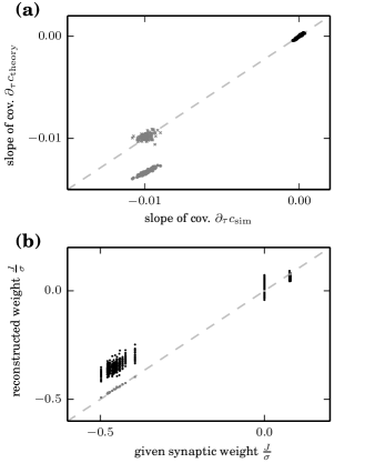
Figure 8: Reconstruction of connectivity from the matrix of covariances and slopes of the covariance functions at zero time lag. (a) Slope of auto- (gray) and cross-covariance functions (black) at zero time lag from the Gaussian approximation versus slope taken from simulation results. Dots show the prediction of the linear theory (36), crosses the approximation $-\frac{1}{2}m_{k}(1-m_{k})$ for the slope of auto-covariances. (b) Reconstructed synaptic amplitude $w_{kl}$ in a network of Ornstein-Uhlenbeck processes (37) (gray) and reconstructed weights $J_{kl}/\sigma_{k}$ (40) (black) in a binary network versus original couplings used in simulation. Covariance and slope averaged over $20$ repetitions, each simulated for $T=2,000,000\>\mathrm{ms}$. Other network parameters as in Figure 1.

Related methods for systems with sequential Glauber update in discrete time steps have previously been proposed. Mézard and Sakellariou (2011) present a method that relates the equal time and one step delayed covariance matrices to the connectivity (see their eqs. (8) and (18)). A similar approach, termed TAP, is described in (Zheng et al., 2011, see their eq. (14)). In contrast, in the time-continuous case considered here, the sum of the covariance function and its slope appear on the left hand side of (38). Qualitatively, the results for discrete and for continuous dynamics agree, as the latter sum presents the first order Taylor approximation of the covariance function at a time lag $\tau$, which is equal to the average update interval.

IX Discussion

We here present a theoretical description of fluctuations in strongly coupled networks of large numbers of binary units that, for the first time, faithfully captures the statistics of individual units as well as pairs of units. The fluctuations are characterized by self-consistent equations for mean activity and pairwise correlations, including finite-size effects down to hundreds of units. The method can be applied to a wide range of networks, in particular networks with asymmetric and strong couplings.

Standard approaches describing symmetric systems in terms of a partition function cannot be extended to non-symmetric coupling, because these systems do not reach thermodynamic equilibrium. Here, we set out to capture the statistics of the system in terms of the cumulant hierarchy for the activity variables. Truncating the hierarchy after second order yields a closed set of equations that already provides a good approximation for the zero time lag covariances between individual units. We show the equivalence of this truncation to the Gaussian approximation of the input field (van Vreeswijk and Sompolinsky, 1998; Renart et al., 2010), which follows from the central limit theorem. Non-Gaussian, finite-size effects in networks of only several hundreds of units are effectively taken into account by incorporating a subset of third order cumulants that can be expressed in terms of lower order cumulants due to the binary nature of the activity variables. This significantly improves the prediction of mean activities, which are strongly affected by the non-linearity of the gain function. The resulting set of non-linear coupled equations can efficiently be solved numerically by damped fixed-point iteration.

We demonstrate that a Heaviside activation function - independent of the choice of coupling amplitudes - constitutes the strongest possible interaction for binary networks. This finding generalizes the invariance of population-averaged pairwise correlations under proportional scaling of couplings and threshold of all units (Grytskyy et al., 2013a; van Albada et al., 2015) to the invariance of individual pairwise correlations under the scaling of the corresponding units’ parameters. Weaker coupling in binary networks can only be achieved by a smoother activation function, but not by different scalings of coupling amplitudes, as e.g. $1/N$ versus $1/\sqrt{N}$, contradictory to frequently employed arguments in the literature (as discussed in van Albada et al., 2015). While the scaling invariance is generic, the presented Gaussian and close-to-Gaussian approximations of the input field hold for the commonly considered narrowly distributed couplings. For wide distributions, the statistics of the input field is likely to depart from the close-to Gaussian assumption.

The contribution of cross-covariances to the marginal statistics of the input to each neuron causes a distribution of the mean activities, even in networks composed of neurons each receiving an identical number of inputs. The classical treatment of neurons with a Heaviside non-linearity neglects this effect (van Vreeswijk and Sompolinsky, 1998). Still, distributed numbers of synaptic inputs typically dominate the distribution of mean activities in sparsely (van Vreeswijk and Sompolinsky, 1998) and densely connected random networks (Renart et al., 2010; Helias et al., 2014).

The Gaussian closure, i.e. the truncation of the cumulant hierarchy after second order, yields a set of equations that accurately predicts the second order statistics. This is in line with experimental evidence showing that pairwise correlations sufficiently constrain maximum entropy models of collective activity (Schneidman et al., 2006). Analogously, the truncation after first order, i.e. the Curie-Weiss mean-field theory that neglects fluctuations altogether, already yields a good estimate of the first moments. In the context of balanced networks this description is sometimes referred to as “balance equations” (van Vreeswijk and Sompolinsky, 1998, eqs. (4.1) and (4.2)). Taking into account fluctuations in the input, due to the variance of individual units (van Vreeswijk and Sompolinsky, 1998), constitutes an intermediate step in the cumulant hierarchy. The variance can be determined exploiting the binary character of the variables resulting in all cumulants of a single unit being fixed by the mean. A consequence of the lower order moments depending only weakly on the statistics of higher order moments is that cross-covariances can be determined from linear fluctuations around the steady state that itself is determined neglecting correlations altogether. We may therefore speculate that an approximation of third or higher order correlations can be obtained from the fluctuations around a state that itself is determined self-consistently by taking into account only up to second order correlations.

The consistent truncation of the cumulant hierarchy further provides deeper insights: The expression for covariances between individual neuron pairs follows naturally from a consistent Gaussian closure, without further approximation. In previous studies, it was obtained as a linear approximation for weak correlations (Renart et al., 2010, supplementary eqs. (31)-(33)) and population-averaged covariances (Ginzburg and Sompolinsky, 1994, eq. (6.8)). We here show that solving the modified Lyapunov equation naturally leads to a decomposition of fluctuations into eigenmodes of the system. The presented method solves the problem that the modified Lyapunov equation does not hold on the diagonal, in contrast to the case of population averages (Ginzburg and Sompolinsky, 1994). The approach moreover exposes that fluctuations in the Gaussian approximation are described by a set of coupled Ornstein-Uhlenbeck processes. It is well known that the fluctuations obtained from a systematic system-size expansion (van Kampen, 1992b, chapter X), to lowest order, obey a Langevin equation. This result has been applied to networks of homogeneous populations (Ohira and Cowan, 1997; Bressloff, 2009; Grytskyy et al., 2013b). The interesting point here is the feasibility of such a reduction directly on the level of individual binary variables. In contrast to the population-averaged activity, the jumps of a binary variable cannot be considered small compared to its value, hence the precondition to apply the system-size expansion is not valid. The approach taken here to expose the correspondence between binary dynamics and Ornstein-Uhlenbeck processes is hence complementary. In particular, the result shows that the effective noises appearing in the equivalent set of Ornstein-Uhlenbeck processes are not uniquely determined by the activities of the neurons alone, in contrast to the population-averaged case (Grytskyy et al., 2013b, sec. 3.1).

Decomposing externally applied signals to the network into the same eigenmodes as the intrinsically generated fluctuations, we obtain an expression for the susceptibility of the network on the single unit level that explains the spatio-temporal filtering applied to external signals, complementing the result for interacting populations (Ginzburg and Sompolinsky, 1994, sec. V). The expression shows how the decay properties of the induced network response are determined by the eigenvalue associated to the eigendirections stimulated by the external signal. In particular, stimuli exciting modes close to an instability yield responses with a long memory life time. In Erdős-Rényi random binary networks with fixed weights, the spectral radius of the linearized connectivity matrix is bounded by $\sqrt{2(1-p)/\pi}<0.8<1$ (Grytskyy et al., 2013a), so that all modes of the network are stable. An instability of the mean activities can only be achieved with connectivity statistics or motifs that differ from an Erdős-Rényi network. This finding is in qualitative contrast to spiking networks that indeed show a rate instability at a critical coupling weight (Ostojic, 2014; Harish and Hansel, 2015). This insight has consequences for the use of random networks with fixed weights in the framework of reservoir computing (Jaeger, 2001; Maass et al., 2002), where highest computational performance (Crutchfield and Young, 1989) is achieved at the edge of chaos (for a review, see Legenstein and Maass, 2007).

We show that the effective interaction strength, i.e. the product of a unit’s susceptibility and the incoming coupling amplitude, can uniquely be reconstructed from the covariance matrix and the slope of the covariance functions at zero time lag. This relation builds on the regression theorem (Risken, 1996), which states that the fluctuations in the system, to linear order (31), follow the same differential equation as the time-delayed covariance functions (2). Coupling amplitudes, for principle reasons, cannot be inferred unambiguously: Correlations only depend on $J/\sigma$, where $\sigma$ measures the strength of the overall incoming fluctuations to the node. The inference of the effective interaction strength $J/\sigma$ still allows the classification of connections into excitatory and inhibitory ones, but leads to a considerable rate of false positive connections. The method presented here requires the measurement of covariances between all pairs of units in the network. In case of severe undersampling, its application is restricted to small sub-networks. Thus, in general settings, more sophisticated approaches that take into account the influence of hidden units on the observed covariances, as e.g. in Tyrcha and Hertz (2013) are more promising. The presented expressions that relate the covariance matrix and its slope at zero time lag to the connectivity may still proof useful to construct similar inference methods for the investigated class of networks. Moreover, the algorithm constructing a network that generates activity with desired mean activities and covariances is a useful tool to generate surrogate data.

Previous works have addressed several aspects of pairwise correlations. The smallness of the average magnitude of covariances in strongly coupled balanced networks (van Vreeswijk and Sompolinsky, 1996) has been explained by the influential work of Renart et al. (2010) in the large $N$ limit. In general, decorrelation follows from the dominant negative feedback in balanced networks at any network size (Tetzlaff et al., 2012; Helias et al., 2014). These global properties are determined by collective fluctuations and can hence be described by population-averaged mean-field theory (Ginzburg and Sompolinsky, 1994). Here we discuss the statistics of individual units, which therefore goes beyond the existing approaches.

Our results are complementary to the method presented in Buice et al. (2009), who consider Markov systems of interacting populations of neurons that consequently have integer numbers of active states, as opposed to the Glauber dynamics (Glauber, 1963) of individual neurons considered here. In consequence, the truncation in the former work is performed on the level of normal-ordered cumulants, that represent an approximation around Poisson statistics, while here we derive an expansion in terms of ordinary cumulants (Gardiner, 2004). Moreover, Buice et al. (2009) rely on a smooth activation function, while our results are generally applicable, including deterministic single units with hard thresholds. Both formalisms generalize to higher order cumulants of activity variables.

A different approach treating the statistics of individual units in a single network realization analytically originates in the spin glass literature. Initiated by the symmetrically coupled Sherrington-Kirkpatrick spin glass model (Sherrington and Kirkpatrick, 1975), an expansion of the free energy in the coupling strength (Plefka-expansion (Plefka, 1982)) leads to the Thouless-Anderson-Palmer mean-field theory (Thouless et al., 1977; Nakanishi and Takayama, 1997; Tanaka, 1998; Nishimori, 2001). By construction this method is restricted to weak coupling and, in its original form, starting from the partition function, also to systems in thermodynamic equilibrium. An extension to asymmetrically coupled non-equilibrium systems has been derived invoking information theoretic arguments (Kappen and Spanjers, 2000). A related approach has been taken by (Zheng et al., 2011). Still, the extended methods rely on the smoothness of the activation function and the smallness of the coupling constants, two restrictions that we are able to overcome here. Compared to previously mentioned works, the presented approach is closer related to the mean-field theory by Mézard and Sakellariou (2011). Although they consider a system with sequential Glauber update in discrete time steps, the method can be extended to the asynchronous update investigated here. Their analysis does not require weak coupling, similar to ours, but in contrast still relies on a smooth activation function for individual units. Moreover, their theory neglects the influence of the cross-covariance on the marginal statistics (their eq. (4)), an important finite-size effect here shown to result in a distribution of mean activities due to correlations alone.

The mean-field methods employed in computer science, biology, artificial intelligence, social sciences, economics, and theoretical neuroscience (see e.g. Fernández-Gracia et al., 2014; Aljadeff et al., 2015; Kadmon and Sompolinsky, 2015) may be complemented by our results that go beyond population-averaged dynamics. The general formalism starting from the master equation can be widely adapted by defining model-specific transition rates (see Tab. 1 in Gleeson, 2013). In neuroscience, with the advancement of electrophysiology, experimental data with hundreds of simultaneously recorded neurons has become readily available (Buzsaki, 2004; Brown et al., 2004). The availability of parallel data progressively changes the focus in neuroscience from the study of single cell responses to emergent phenomena arising through the interaction between neurons in networks (Stevenson and Kording, 2011). Pairwise correlations are moreover closely linked to fluctuations of the population activity (Tetzlaff et al., 2012), which have been shown to shape experimentally accessible signals, such as the local field potential or the electroencephalogram (EEG) (Lindén et al., 2011; Mazzoni et al., 2010). The effective description of the statistics of individual neurons, valid in the entire range of coupling strength, forms the basis for studies of dynamics on adaptive networks (Gross et al., 2006), e.g. the interaction of neuronal dynamics with correlation-sensitive learning rules (Ocker et al., 2015). Explicit expressions not only for zero time lag, but also for the slope of covariance functions allow the definition of plasticity rules resembling spike-timing dependent plasticity (Morrison et al., 2008). The finding that the collective dynamics is captured by the non-trivial second order statistics implies that theoretical descriptions of mechanisms, e.g. biologically realistic synaptic learning, which usually only rely on first and second order statistics, have now come into reach. Balanced networks show widely distributed correlations across pairs of neurons with small mean (Ecker et al., 2010). This robust feature is captured by the presented linear equations for the covariance matrix. The shape of the distribution has to date not been related to the properties of the underlying network structure. Further work is required to obtain analytical expressions exposing how the structural properties give rise to the statistics of the distribution of covariances. Such results would enable us to deduce statistics of the connections from the observed activity. The presented description of the structure of fluctuations in this archetypical model of collective phenomena by a set of non-linear equations provides a starting point in this endeavor and facilitates further development on disordered, coupled systems with large numbers of degrees of freedom.

X Appendix

X.1 Derivation of moment equations up to second order

For completeness and to establish a consistent notation, we here include the derivation of equations (2) for the first and second moments of the activity in a binary network. We follow the notation introduced in Buice et al. (2009) and used in Helias et al. (2014).

The stochastic system is completely characterized by the joint probability distribution $p(\mathbf{n})$ of all $N$ binary variables $\mathbf{n}$. Knowing the joint probability distribution, arbitrary moments can be calculated, among them pairwise correlations. The occupation probability of each state follows the master equation (41). We denote as $\mathbf{n}_{i+}=(n_{1},\ldots,n_{i-1},1,n_{i+1},\ldots,n_{N})$ the state, where the $i$-th neuron is active ($n_{i}=1$), and $\mathbf{n}_{i-}$ where neuron $i$ is inactive ($n_{i}=0$). Since in each infinitesimal time interval at most one neuron can change state, for each given state $\mathbf{n}$ there are $N$ possible transitions (each corresponding to one of the $N$ neurons changing state). The sum of the probability fluxes into the state and out of the state must sum up to the change of probability in the respective state (Kelly, 1979), i.e.

$$\tau\frac{\partial p(\mathbf{n})}{\partial t}= \sum_{i=1}^{N}(2n_{i}-1)\left(p(\mathbf{n}_{i-})F_{i}(\mathbf{n}_{i-})\right.$$

$$\hphantom{\sum_{i=1}^{N}(2n_{i}-1)}-\left.p(\mathbf{n}_{i+})(1-F_{i}(\mathbf{n}_{i+})\right)$$ (41)

$\forall\quad\mathbf{n}\in\{0,1\}^{N}.$ From this equation we derive expressions for the first $\langle n_{k}\rangle$ and second moments $\langle n_{k}n_{l}\rangle$ by multiplying with $n_{k}n_{l}$ and summing over all possible states $\mathbf{n}\in\{0,1\}^{N}$, which leads to

$$\tau\frac{\partial}{\partial t}\langle n_{k}n_{l}\rangle = \sum_{\mathbf{n}\in\{0,1\}^{N}}\sum_{i=1}^{N}n_{k}n_{l}(2n_{i}-1)$$

$$\times\underbrace{\left(p(\mathbf{n}_{i-})F_{i}(\mathbf{n}_{i-})-p(\mathbf{n}_{i+})(1-F_{i}(\mathbf{n}_{i+}))\right)}_{\equiv G_{i}(\mathbf{n}\backslash n_{i})},$$

where we denote as $\langle f(\mathbf{n})\rangle=\sum_{\mathbf{n}\in\{0,1\}^{N}}p(\mathbf{n})f(\mathbf{n})$ the average of a function $f(\mathbf{n})$ with respect to the distribution $p(\mathbf{n})$. Note that the term denoted $G_{i}(\mathbf{n}\backslash n_{i})$ does not depend on the state of neuron $i$. We use the notation $\mathbf{n}\backslash n_{i}$ for the state of the network excluding neuron $i$, i.e. $\mathbf{n}\backslash n_{i}=(n_{1},\ldots,n_{i-1},n_{i+1},\ldots,n_{N})$. Separating the terms in the sum over $i$ into those with $i\neq k,l$ and the two terms with $i=k$ and $i=l$, we obtain

$$\tau\frac{\partial}{\partial t}\langle n_{k}n_{l}\rangle = \sum_{\mathbf{n}}\;\sum_{i=1,i\neq k,l}^{N}n_{k}n_{l}(2n_{i}-1)\,G_{i}(\mathbf{n}\backslash n_{i})$$

$$\hphantom{\sum_{\mathbf{n}}\;\sum_{i=1,i\neq k,l}^{N}}+n_{k}n_{l}(2n_{k}-1)\,G_{k}(\mathbf{n}\backslash n_{k})$$

$$\hphantom{\sum_{\mathbf{n}}\;\sum_{i=1,i\neq k,l}^{N}}+n_{k}n_{l}(2n_{l}-1)\,G_{l}(\mathbf{n}\backslash n_{l})$$

$$= \sum_{i=1,i\neq k,l}^{N}\;\sum_{\mathbf{n}\backslash n_{i}}n_{k}n_{l}(G_{i}(\mathbf{n}\backslash n_{i})-G_{i}(\mathbf{n}\backslash n_{i}))$$

$$+\sum_{\mathbf{n}}n_{k}n_{l}\,G_{k}(\mathbf{n}\backslash n_{k})+\sum_{\mathbf{n}}n_{k}n_{l}\,G_{l}(\mathbf{n}\backslash n_{l}),$$

where we obtained the first term by explicitly summing over state $n_{i}\in\{0,1\}$ (i.e. using $\sum_{\mathbf{n}\in\{0,1\}^{N}}=\sum_{\mathbf{n}\backslash n_{i}\in\{0,1\}^{N-1}}\sum_{n_{i}=0}^{1}$ and evaluating the sum $\sum_{n_{1}=0}^{1}$). This first sum obviously vanishes. The remaining terms are of identical form with the roles of $k$ and $l$ interchanged. We hence only consider the first of them and obtain the other by symmetry. The first term simplifies to

$$\sum_{\mathbf{n}}n_{k}n_{l}\,G_{k}(\mathbf{n}\backslash n_{k})$$ (42)

$$\stackrel{{\scriptstyle\text{${\scriptstyle\mbox{$n_{k}=1$}}$}}}{{=}} \sum_{\mathbf{n}\backslash n_{k}}n_{l}\,G_{k}(\mathbf{n}\backslash n_{k})$$

$$\stackrel{{\scriptstyle\text{${\scriptstyle\text{def. }\mbox{$G_{k}$}}$}}}{{=}} \begin{cases}\sum_{\mathbf{n}\backslash n_{k}}p(\mathbf{n}_{k-})\,F_{k}(\mathbf{n}_{k-})\\ \hphantom{\sum_{\mathbf{n}\backslash n_{k}}}+p(\mathbf{n}_{k+})\,F_{k}(\mathbf{n}_{k+})-p(\mathbf{n}_{k+})&\text{for }k=l\\ \sum_{\mathbf{n}\backslash n_{k}}p(\mathbf{n}_{k-})\,n_{l}\,F_{k}(\mathbf{n}_{k-})\\ \hphantom{\sum_{\mathbf{n}\backslash n_{k}}}+p(\mathbf{n}_{k+})\,n_{l}\,F_{k}(\mathbf{n}_{k+})-n_{l}\,p(\mathbf{n}_{k+})&\text{for }k\neq l\end{cases}$$

$$= \begin{cases}\langle F_{k}(\mathbf{n})\rangle-\langle n_{k}\rangle&\text{for }k=l\\ \langle F_{k}(\mathbf{n})\,n_{l}\rangle-\langle n_{k}n_{l}\rangle&\text{for }k\neq l\end{cases}.$$

Taken together with the mirror term $k\leftrightarrow l$, we arrive at two conditions, one for the first ($k=l$, $\langle n_{k}^{2}\rangle=\langle n_{k}\rangle$) and one for the second ($k\neq l$) moment

$$\tau\frac{\partial}{\partial t}\langle n_{k}\rangle \stackrel{{\scriptstyle\text{${\scriptstyle\mbox{$k=l$}}$}}}{{=}}-\langle n_{k}\rangle+\langle F_{k}(\mathbf{n})\rangle$$ (43)

$$\tau\frac{\partial}{\partial t}\langle n_{k}n_{l}\rangle \stackrel{{\scriptstyle\text{${\scriptstyle\mbox{$k\neq l$}}$}}}{{=}}-2\langle n_{k}n_{l}\rangle+\langle F_{k}(\mathbf{n})\,n_{l}\rangle+\langle F_{l}(\mathbf{n})\,n_{k}\rangle.$$ (44)

The time-lagged correlation function can be derived along completely analogous lines as (44), as the forward time evolution equation (differential equation with respect to $t$) of the two point probability distribution $p(\mathbf{n},t,\mathbf{q},s)$ fulfills, due to the Markov property, the same master equation (41) as the equal time probability distribution $p(\mathbf{n},t)$. The resulting differential equation reads

$$\tau\frac{\partial}{\partial t}\langle n_{k}(t)n_{l}(s)\rangle \equiv\sum_{\mathbf{n},\mathbf{q}}p(\mathbf{n},t,\mathbf{q},s)\,n_{k}q_{l}$$

$$=\ldots$$

$$=-\langle n_{k}(t)n_{l}(s)\rangle+\langle F_{k}(\mathbf{n}(t))\,n_{l}(s)\rangle.$$ (45)

X.2 Cumulants of summed random variables

Let

$$y = \sum_{i=1}^{N}x_{i},$$ (46)

with $x_{i}$ random variables that follow an arbitrary distribution $p(\mathbf{x})$. The moment generating functions of $y$ and $\mathbf{x}$ are then related by

$$\varphi_{y}(t) = \sum_{\mathbf{x}}p(\mathbf{x})e^{ty}=\langle e^{ty}\rangle_{\mathbf{x}}$$

$$= \langle e^{t\sum_{i=1}^{N}x_{i}}\rangle_{\mathbf{x}}$$

$$= \left(\varphi_{\mathbf{x}}\circ\iota\right)(t),$$

where concatenation with the function $\iota:t\mapsto(t,\ldots,t)$ replaces every $t_{i}$ by a $t$. The cumulant generating functions therefore follow as

$$\Phi_{y}(t) = \ln\varphi_{y}(t)$$ (48)

$$= \ln\left(\varphi_{\mathbf{x}}\circ\iota\right)(t)=\left(\Phi_{\mathbf{x}}\circ\iota\right)(t),$$

with $\Phi_{\mathbf{x}}(\mathbf{t})=\ln\langle e^{\mathbf{t}\cdot\mathbf{x}}\rangle$ the cumulant generating function of the $\mathbf{x}$ and $\mathbf{t}\cdot\mathbf{x}$ the scalar product. From the expansion in cumulants $\kappa_{ij\ldots}^{x}$ for $\mathbf{x}$ and $\kappa_{1,2,\ldots}$ for $y$ follows the relationship

$$\Phi_{y}(t) \equiv \sum_{l=1}^{\infty}\frac{\kappa_{l}}{l!}t^{l}$$ (49)

$$= \left(\Phi_{\mathbf{x}}\circ\iota\right)(t)$$

$$= \left[\left(\sum_{i=1}^{N}\kappa_{i}^{x}t_{i}+\sum_{i,j=1}^{N}\frac{\kappa_{ij}^{x}}{2!}\,t_{i}t_{j}+\ldots\right)\circ\iota\right](t)$$

$$= \underbrace{\sum_{i=1}^{N}\kappa_{i}^{x}}_{\kappa_{1}}\,t+\frac{1}{2!}\underbrace{\sum_{i,j=1}^{N}\kappa_{ij}^{x}}_{\kappa_{2}}\,t^{2}+\ldots,$$

so the cumulants of the summed variable $\kappa_{1}$, $\kappa_{2}$, etc are given by the sums of the cumulants of the individual variables of corresponding order.

X.3 Functions of close-to Gaussian variables

To determine the mean activity, we need to apply a non-linear function $f$ to a variable $h_{k}$ that has a statistics which is close to Gaussian. For brevity, we will suppress the index $k$ in the following. We assume that the Fourier transform $\hat{f}(\omega)$ exists. Let $y$ be the random variable (46) which is a sum of a large number of individual variables $x_{i}$ and is assumed to be close to Gaussian. For the expectation value $\langle f(y)\rangle_{y}$ we get

$$\langle f(y)\rangle_{\mathbf{x}} =\frac{1}{2\pi}\int d\omega\,\hat{f}(\omega)\,\langle e^{i\omega y}\rangle_{\mathbf{x}}$$

$$=\frac{1}{2\pi}\int d\omega\,\hat{f}(\omega)\,e^{\Phi_{y}(i\omega)}$$

$$=\frac{1}{2\pi}\int d\omega\,\hat{f}(\omega)\,e^{\kappa_{1}(i\omega)+\frac{1}{2!}\kappa_{2}(i\omega)^{2}+\frac{1}{3!}\kappa_{3}(i\omega)^{3}+\ldots},$$ (50)

where $\Phi_{y}$ is the cumulant generating function of $y$ (48) and $\kappa_{i}$ denotes the $i$-th cumulant of $y$. We are interested in an approximation that treats the dominant first and second (Gaussian) cumulants of $y$ explicitly and separate the effect of all higher cumulants by writing

$$\langle f(y)\rangle_{\mathbf{x}} = e^{\frac{1}{6}\kappa_{3}\left(\frac{\partial}{\partial\kappa_{1}}\right)^{3}+\ldots}\int d\omega\,\hat{f}(\omega)\,e^{\kappa_{1}(i\omega)+\frac{1}{2}\kappa_{2}(i\omega)^{2}}$$ (51)

$$= e^{\frac{1}{6}\kappa_{3}\left(\frac{\partial}{\partial\kappa_{1}}\right)^{3}+\ldots}\langle f(y)\rangle_{y\sim\mathcal{N}(\kappa_{1},\kappa_{2})},$$

where we identified in the last line the Fourier transform of a Gaussian with moments $\kappa_{1}$ and $\kappa_{2}$ via (50).

For the covariance we need to evaluate terms of the form $\langle F_{k}n_{l}\rangle$. These terms can be obtained analogously as

$$\langle f(y)x_{l}\rangle_{\mathbf{x}} = \frac{1}{2\pi}\int d\omega\,\hat{f}(\omega)\,\langle x_{l}\,e^{i\omega y}\rangle_{\mathbf{x}}$$

$$= \frac{1}{2\pi}\int d\omega\,\hat{f}(\omega)\,\left(\left(\partial_{t_{l}}\varphi_{\mathbf{x}}\right)\circ\iota\right)(i\omega)$$

$$= \frac{1}{2\pi}\int d\omega\,\hat{f}(\omega)\,\left(\left(\left[\partial_{t_{l}}\Phi_{\mathbf{x}}\right]\,e^{\Phi_{\mathbf{x}}}\right)\circ\iota\right)(i\omega),$$

where $\varphi_{\mathbf{x}}$ is the moment generating function of $\mathbf{x}$ (X.2). The derivative of the cumulant generating function with (49) becomes

$$\partial_{t_{l}}\Phi_{\mathbf{x}}(\mathbf{t}) = \kappa_{l}^{x}+\sum_{j=1}^{N}\kappa_{lj}^{x}\,t_{j}+\frac{1}{2}\sum_{i,j=1}^{N}\kappa_{lij}^{x}\,t_{i}t_{j}+\ldots$$

$$\left(\partial_{t_{l}}\Phi_{\mathbf{x}}\circ\iota\right)(i\omega) = \kappa_{l}^{x}+\underbrace{\sum_{j=1}^{N}\kappa_{lj}^{x}}_{=:\Delta\kappa_{1,l}}\,(i\omega)+\frac{1}{2}\underbrace{\sum_{i,j=1}^{N}\kappa_{lij}^{x}}_{=:\Delta\kappa_{2,l}}\,(i\omega)^{2}+\ldots$$

$$= \sum_{q=0}^{\infty}\Delta\kappa_{q,l}(i\omega)^{q},$$

where product rule produced a factor $2$ in the second term and a factor $3$ in the third term and we used the symmetry of the cumulants with respect to permutations of indices. So we get

$$\langle x_{l}f(y)\rangle_{\mathbf{x}} = \int d\omega\,\hat{f}(\omega)\,\sum_{q=0}^{\infty}\Delta\kappa_{q,l}(i\omega)^{q}e^{\sum_{p=0}^{\infty}\kappa_{p}(i\omega)^{p}}$$ (52)

$$= \left[\sum_{q=0}^{\infty}\Delta\kappa_{q,l}\,\frac{\partial}{\partial\kappa_{q}}\right]\,e^{\frac{1}{3!}\kappa_{3}\left(\frac{\partial}{\partial\kappa_{1}}\right)^{3}+\ldots}\langle f(y)\rangle_{y\sim\mathcal{N}(\kappa_{1},\kappa_{2})}$$

$$= \left[\sum_{q=0}^{\infty}\Delta\kappa_{q,l}\,\frac{1}{q!}\,\left(\frac{\partial}{\partial\kappa_{1}}\right)^{q}\right]\,\langle f(y)\rangle_{\mathbf{x}},$$

where we replaced $(i\omega)^{q}$ by derivatives of the exponential with respect to cumulants and identified $\langle f(y)\rangle_{\mathbf{x}}$ in the last step using (51).

X.4 Trivial third and fourth order cumulants of binary variables expressed by lower order cumulants

Third order. Let $n_{l},n_{i},n_{j},n_{r}\in[0,1]$ be binary variables. The raw third moment can be written as a sum of all combinations of cumulants up to order three (IV) $\langle n_{l}n_{i}n_{j}\rangle=\llangle n_{l}n_{i}n_{j}\rrangle+c_{li}m_{j}+c_{ij}m_{l}+c_{jl}m_{i}+m_{l}m_{i}m_{j}.$ Using $n_{i}^{K}=n_{i}$ for each integer $K\geq 1$, in case of binary variables $n_{i}$ we consider the two cases

$$l=i\neq j:\quad\langle n_{l}n_{j}\rangle = \llangle n_{l}n_{l}n_{j}\rrangle$$

$$+ c_{ll}m_{j}+c_{lj}m_{l}+c_{jl}m_{l}$$

$$+ m_{l}^{2}m_{j}$$

$$\llangle n_{l}n_{l}n_{j}\rrangle = \underbrace{\langle n_{l}n_{j}\rangle}_{c_{lj}+\langle n_{l}\rangle\langle n_{j}\rangle}-c_{ll}m_{j}-2c_{lj}m_{l}-m_{l}^{2}m_{j}$$

$$= c_{lj}(1-2m_{l})+(\underbrace{-c_{ll}+m_{l}-m_{l}^{2}}_{=0})m_{j}$$

$$= c_{lj}(1-2m_{l})$$

$$l=i=j:\quad\langle n_{l}\rangle = \llangle n_{l}n_{l}n_{l}\rrangle+3c_{ll}m_{l}+m_{l}^{3}$$

$$\llangle n_{l}n_{l}n_{l}\rrangle = m_{l}-3m_{l}(1-m_{l})m_{l}-m_{l}^{3}$$ (53)

$$= m_{l}-3m_{l}^{2}+2m_{l}^{3}$$

$$= c_{ll}(1-2m_{l}),$$

which together yield the expression (21) in the main text.

The third cumulant (17) of $h_{k}$ follows with the assumption $\llangle n_{i}n_{j}n_{r}\rrangle\simeq 0$ for $i\neq j\neq r$ as

$$\kappa_{3,k} = \sum_{ijr}J_{ki}J_{kj}J_{kr}\llangle n_{i}n_{j}n_{r}\rrangle$$ (54)

$$= \underbrace{\sum_{i\neq j\neq r}}_{N(N-1)(N-2)\text{ terms}}J_{ki}J_{kj}J_{kr}\underbrace{\llangle n_{i}n_{j}n_{r}\rrangle}_{\simeq 0}$$

$$+3\underbrace{\sum_{i=j\neq r}}_{N(N-1)\text{ terms}}J_{ki}^{2}J_{kr}\llangle n_{i}n_{i}n_{r}\rrangle+\underbrace{\sum_{i=j=r}}_{N\text{ terms}}J_{ki}^{3}\llangle n_{i}n_{i}n_{i}\rrangle$$

$$\simeq 3\sum_{i=j\neq r}J_{ki}^{2}J_{kr}c_{ir}(1-2m_{i})+\sum_{i=j=r}J_{ki}^{3}c_{ii}(1-2m_{i})$$

$$= 3\sum_{i,r}J_{ki}^{2}(1-2m_{i})c_{ir}J_{kr}-2\sum_{i}J_{ki}^{3}c_{ii}(1-2m_{i}),$$

where we included the term $i=r$ in the first sum and compensated accordingly in the latter term. With $c_{ii}(1-2m_{i})=m_{i}-3m_{i}^{2}+2m_{i}^{3}$ we obtain the expression (22) in the main text. Analogously follows

$$\sum_{i,j=1}^{N}J_{ki}J_{kj}\llangle n_{l}n_{i}n_{j}\rrangle$$ (55)

$$= \underbrace{\sum_{i\neq j\neq l}J_{ki}J_{kj}\llangle n_{l}n_{i}n_{j}\rrangle}_{\simeq 0}+\sum_{l\neq i=j=1}^{N}J_{ki}^{2}\llangle n_{l}n_{i}n_{i}\rrangle$$

$$+\sum_{i=l\neq j=1}^{N}J_{kl}J_{kj}\llangle n_{l}n_{l}n_{j}\rrangle+\sum_{j=l\neq i=1}^{N}J_{ki}J_{kl}\llangle n_{l}n_{i}n_{l}\rrangle$$

$$+J_{kl}^{2}\llangle n_{l}n_{l}n_{l}\rrangle$$

$$= \sum_{l\neq i=1}^{N}J_{ki}^{2}\,c_{li}(1-2m_{i})+2J_{kl}\,\sum_{l\neq i=1}^{N}J_{ki}c_{li}(1-2m_{l})$$

$$+J_{kl}^{2}c_{ll}(1-2m_{l})$$

$$= \sum_{i=1}^{N}J_{ki}^{2}\,(1-2m_{i})c_{li}+2J_{kl}\,(1-2m_{l})\sum_{i=1}^{N}J_{ki}c_{li}$$

$$-2J_{kl}^{2}\,c_{ll}(1-2m_{l}),$$

which yields the expression (23) in the main text.

Fourth order. The cumulant of fourth order is

$$\langle n_{i}n_{j}n_{r}n_{l}\rangle = \llangle n_{i}n_{j}n_{r}n_{l}\rrangle$$

$$+\llangle n_{i}n_{j}n_{r}\rrangle m_{l}+\llangle n_{j}n_{r}n_{l}\rrangle m_{i}$$

$$+\llangle n_{r}n_{l}n_{i}\rrangle m_{j}+\llangle n_{l}n_{i}n_{j}\rrangle m_{r}$$

$$+c_{ij}m_{r}m_{l}+c_{ir}m_{j}m_{l}+c_{il}m_{r}m_{j}$$

$$+c_{jr}m_{l}m_{i}+c_{jl}m_{r}m_{i}+c_{rl}m_{i}m_{j}$$

$$+c_{ij}c_{rl}+c_{ir}c_{jl}+c_{il}c_{rj}$$

$$+m_{i}m_{j}m_{r}m_{l},$$

Only those cumulants in which at most two different indices appear are fixed by first and second order cumulants. We need to distinguish three cases. The first case is $i=j\neq r=l$ and leads with (53) to the matrix

$$\left\{\llangle n_{i}n_{i}n_{r}n_{r}\rrangle_{ir}\right\} = \mathbf{C}\circledast(\mathbf{1}-2\mathbf{C})-\mathrm{diag}(\mathbf{C})\,\mathrm{diag}(\mathbf{C})^{T}$$ (56)

$$-2\,\mathrm{diag}(\mathbf{1}-2\mathbf{m}))\,\mathbf{C}\,\mathrm{diag}(\mathbf{m})$$

$$-2\,\mathrm{diag}(\mathbf{m})\,\mathbf{C}\,\mathrm{diag}(\mathbf{1}-2\mathbf{m})$$

$$-\mathrm{diag}(\mathbf{C})\left(\mathbf{m}\circledast\mathbf{m}\right)^{T}-\left(\mathbf{m}\circledast\mathbf{m}\right)\mathrm{diag}(\mathbf{C})^{T}$$

$$-4\,\mathrm{diag}(\mathbf{m})\,\mathbf{C}\,\mathrm{diag}(\mathbf{m})$$

$$+\mathbf{m}\mathbf{m}^{T}\circledast(\mathbf{1}-\mathbf{m}\mathbf{m}^{T}).$$

The second case $i=j=l\neq r$ yields the matrix

$$\left\{\llangle n_{i}n_{i}n_{i}n_{r}\rrangle_{ir}\right\} = \mathrm{diag}(\mathbf{1}-3\,\mathrm{diag}(\mathbf{C}))\,\mathbf{C}$$ (57)

$$-\mathrm{diag}(\mathbf{C})\mathbf{m}^{T}-3\,\mathrm{diag}(\mathbf{m})\,\mathbf{C}$$

$$-\left(\mathbf{m}\circledast\mathrm{diag}(\mathbf{C})\right)\,\mathbf{m}^{T}+3\,\mathrm{diag}(\mathbf{m}\circledast\mathbf{m})\,\mathbf{C}$$

$$+\mathrm{diag}(\mathbf{1}-\mathbf{m}\circledast\mathbf{m}))\,\mathbf{m}\mathbf{m}^{T}$$

and the third for $i=j=r=l$ yields a vector

$$\llangle n_{i}n_{i}n_{i}n_{i}\rrangle = \mathbf{m}\circledast(\mathbf{1}-(\mathbf{m}\circledast)^{3})-4\,\mathrm{diag}(\mathbf{C})\circledast\mathbf{m}$$ (58)

$$+2\,\mathrm{diag}(\mathbf{C})\circledast(\mathbf{m}\circledast)^{2}$$

$$-3(\mathrm{diag}(\mathbf{C})\circledast)^{2},$$

where we use the notation$\left(\mathbf{x}\circledast\right)^{n}=\mathbf{x}\circledast\ldots\circledast\mathbf{x}$ for the element-wise $n$-th power of a vector. In (19) we need the term

$$\Delta\kappa_{3,kl} = \sum_{i,j,r=1}^{N}J_{ki}J_{kj}J_{kr}\llangle n_{i}n_{j}n_{r}n_{l}\rrangle$$

$$\simeq 3\sum_{i}J_{ki}^{2}J_{kl}\llangle n_{i}n_{i}n_{l}n_{l}\rrangle\qquad{\scriptstyle\left(i=j,r=l\right),\left(i=r,j=l\right),\left(i=l,j=r\right)}$$

$$+\sum_{i}J_{ki}^{3}\llangle n_{i}n_{i}n_{i}n_{l}\rrangle\qquad{\scriptstyle\left(i=j=r\neq l\right)}$$

$$+3\sum_{i}J_{ki}J_{kl}^{2}\llangle n_{l}n_{l}n_{l}n_{i}\rrangle\qquad{\scriptstyle\left(j=r=l\neq i\right),\left(r=l=i\neq j\right),\left(l=i=j\neq r\right)}$$

$$+J_{kl}^{3}\llangle n_{l}n_{l}n_{l}n_{l}\rrangle\qquad{\scriptstyle\left(i=j=r=l\right)},$$

which in matrix form gives rise to expression (IV) of the main text.