$K_{0}^{\ast}(800)$ as a companion pole of $K_{0}^{\ast}(1430)$

Abstract

We study the light scalar sector up to $1.8$ GeV by using a quantum field theoretical approach which includes a single kaonic state in a Lagrangian with both derivative and non-derivative interactions. By performing a fit to $\pi K$ phase shift data in the $I=1/2,$ $J=0$ channel, we show that $K_{0}^{\ast}(800)$ (or $\kappa$) emerges as a dynamically generated companion pole of $K_{0}^{\ast}(1430)$. This is a result of investigating quantum fluctuations with one kaon and one pion circulating in the loops dressing $K_{0}^{\ast}(1430)$. We determine the position of the poles on the complex plane in the context of our approach: for $K_{0}^{\ast}(1430)$ we get $(1.413\pm 0.002)-i\hskip 0.56917pt(0.127\pm 0.003)$ (in GeV), while for $\kappa$ we get $(0.746\pm 0.019)-i\hskip 0.56917pt(0.262\pm 0.014)$ (in GeV). The model-dependence of these results and related uncertainties are discussed in the paper. A large-$N_{c}$ study confirms that $K_{0}^{\ast}(1430)$ is predominantly a quarkonium and that $K_{0}^{\ast}(800)$ is a molecular-like dynamically generated state.

I Introduction

The lightest scalar resonance with isospin $I=1/2$ is the state $K_{0}^{\ast}(800)$, also denoted as $\kappa$. This state is not yet listed in the summary table of the Particle Data Group (PDG) Olive et al. (2014). The confirmation of $\kappa$ is important, since it would complete the nonet of light scalar states below $1$ GeV. Namely, besides the putative $\kappa$ state, the broad but by now established $f_{0}(500)$ (see Ref. Peláez (2015) and references therein) as well as the narrow resonances $a_{0}(980)$ and $f_{0}(980)$ are well-established mesons Olive et al. (2014). These light scalar mesons are excellent candidates to be non-conventional states, $i.e.$, four-quark objects, realized as diquark-antidiquark states Jaffe (1977a); *jaffe2; Jaffe (2005); Maiani et al. (2004); Giacosa (2006); *tqmix; *pagliaraderivatives2; Fariborz et al. (2005); *fariborz; *rodriguez; *fariborz3 and/or as dynamically generated molecular-like states Close and Törnqvist (2002); Peláez and Ríos (2006); *pelaez2; Peláez (2004b); Oller and Oset (1997); *oller2; *oller3; Oller and Oset (1999); Jamin et al. (2000); *oller6; van Beveren et al. (2006); Morgan and Pennington (1993); van Beveren et al. (1986); Törnqvist (1995); *tornqvist2; Boglione and Pennington (1997); *pennington (for review, see also Ref. Amsler and Törnqvist (2004); *amslerrev2).

The aim of this work is to apply a quantum field theoretical approach in order to investigate the existence of the $\kappa$ as well as its nature. Within our approach a single (quark-antiquark) seed state, roughly corresponding to the well-known resonance $K_{0}^{\ast}(1430)$, is described by an effective Lagrangian. In particular, we shall use a Lagrangian that contains – in agreement with chiral perturbation theory (chPT) and chiral models – both derivative and non-derivative interaction terms. As we shall see, the simultaneous presence of both of them ensures a good description of scattering data. Indeed, as expected from chPT the derivative interaction gives the largest contribution. After computing the full one-loop resummed propagator we perform a fit to experimental $\pi K$ phase shift data from Ref. Aston et al. (1988). The fit depends on four parameters of the model: two coupling constants, one bare mass, and one cutoff entering a Gaussian form factor. We find that, besides the expected resonance pole of $K_{0}^{\ast}(1430)$, a pole corresponding to the light $\kappa$ naturally emerges on the unphysical Riemann sheet. In this situation the $\kappa$ is established as a dynamically generated companion pole of the conventional quark-antiquark meson $K_{0}^{\ast}(1430)$. We determine the position of the poles for both states including errors. For previous determinations of the pole position of $\kappa$ see $e.g.$ Refs. Ishida et al. (1997); Magalhães et al. (2011); Descotes-Genon and Moussalam (2006); Peláez (2004a, b); Zheng et al. (2004); *zheng2; Black et al. (1998); Fariborz et al. (2015b); Ledwig et al. (2014), as well as the experimental observation by BES Ablikim et al. (2011) and the lattice study of Ref. Fu (2012).

Moreover, $(i)$ it turns out that the light $\kappa$ does not correspond to any peak in the scalar kaonic spectral function but only to an enhancement in the low-energy region at about $750$ MeV. A large-$N_{c}$ study shows that its pole disappears when $N_{c}$ is large enough ($N_{c}\simeq 13$). As a consequence, this state is not predominantly a quarkonium but rather a dynamically generated meson. $(ii)$ On the other hand, the pole of the corresponding state above $1$ GeV tends to the real energy axis in the large-$N_{c}$, as expected for a predominantly quark-antiquark state.

For completeness, we also investigate the statistical significance of our results: we find that both derivative and non-derivative interactions are needed for a satisfactory fit. On the contrary, variations of the models with only derivative or non-derivative interactions or with other form factors different from the Gaussian turn out not to be in agreement with the experimental results.

II The model

Our model consists of an interaction Lagrangian describing the interaction/decay of a single scalar kaonic seed state, denoted as $K_{0}^{\ast}$, into one pion and one kaon. In agreement with effective approaches of low-energy QCD (both chPT Gasser and Leutwyler (1984); *Ecker; *chpt2 and effective chiral models Ko and Rudaz (1994); *ko2; Parganlija et al. (2013), based on the nonlinear and linear realization of chiral symmetry, respectively), it consists of two types of terms, $i.e.$, one without and one involving derivatives:

$$\mathcal{L}_{\text{int}} = aK_{0}^{\ast-}\pi^{0}K^{+}+bK_{0}^{\ast-}\partial_{\mu}\pi^{0}\partial^{\mu}K^{+}$$

$$+\ \sqrt{2}aK_{0}^{\ast-}\pi^{+}K^{0}+\sqrt{2}bK_{0}^{\ast-}\partial_{\mu}\pi^{+}\partial^{\mu}K^{0}+\dots\ ,$$

where dots represent analogous interaction terms for the other members of the isospin multiplets, as well as Hermitian conjugation. The decay width as function of the (running) mass $m$ of the unstable $K_{0}^{\ast}$ reads

$$\Gamma_{K_{0}^{\ast}}(m)=3\hskip 0.56917pt\frac{k(m)}{8\pi m^{2}}\left[a-b\hskip 0.56917pt\frac{m^{2}-m_{\pi}^{2}-m_{K}^{2}}{2}\right]^{2}F_{\Lambda}(m)\ ,$$ (2)

where the factor of $3$ comes from summing over isospin. Here, we introduced the modulus of the three-momentum of the outgoing particles in the rest frame of the decaying particle as

$$k(m) =\frac{\sqrt{m^{4}+\left(m_{\pi}^{2}-m_{K}^{2}\right)^{2}-2\left(m_{\pi}^{2}+m_{K}^{2}\right)m^{2}}}{2m}$$

$$\times\ \theta\left(m-m_{\pi}-m_{K}\right)\ .$$ (3)

The quantities $m_{\pi}$ and $m_{K}$ are the pion and kaon mass, respectively. The form factor $F_{\Lambda}(m)$ is chosen as

$$F_{\Lambda}(m)=e^{-2k^{2}(m)/\Lambda^{2}}\ ,$$ (4)

where $\Lambda$ is an energy scale arising from the fact that mesons are not elementary objects (technically, it can be included already in the Lagrangian by making it non-local, see $e.g.$ Ref. Terning (1991); *nonlocal2). This parameter acts as a cutoff and assures that all our calculations are finite.

When the form factor is set to zero in Eq. (2) and $m\simeq 1.43$ GeV, we obtain the so-called tree-level decay width. It can be identified with the physical width of the $K_{0}^{\ast}(1430)$ in (some) phenomenological models, in which this resonance is interpreted as a quarkonium Parganlija et al. (2013). As we shall see, the bare seed state $K_{0}^{\ast}$ in our Lagrangian (II) in fact corresponds roughly to the well-known resonance $K_{0}^{\ast}(1430)$ – this is in agreement with various phenomenological studies of the scalar sector Fariborz et al. (2005); *fariborz; *rodriguez; *fariborz3; Parganlija et al. (2013); Amsler and Close (1996); *close3; *close7; *close5; Godfrey and Isgur (1985).

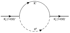
Figure 1: Example of a one-loop contribution to $\Pi(m)$.

Following closely Ref. Wolkanowski et al. (2016) (see also Refs. van Beveren et al. (1986); Törnqvist (1995); *tornqvist2; Boglione and Pennington (1997); *pennington; Giacosa and Pagliara (2007); *e38), we now briefly present the mathematical formalism. The propagator of the scalar kaonic field is given by

$$\Delta_{K_{0}^{\ast}}(p^{2}=m^{2})=\frac{1}{m^{2}-m_{0}^{2}-\Pi(m)+i\varepsilon}\ ,$$ (5)

where $m_{0}$ is the bare mass of the scalar kaon and $\Pi(m)$ is the sum of all one-loop contributions with one pion and one kaon circulating in it, see Fig. 1. Although the loops in our model are regularized by the form factor in Eq. (4), one has to take into account emerging tadpole diagrams when using ordinary Feynman rules. The details are discussed in Ref. Wolkanowski et al. (2016). A study of the validity of the one-loop approximation was done in Ref. Schneitzer et al. (2014). We will use that the spectral function is obtained from the propagator by

$$d_{K_{0}^{\ast}}(m)=-\frac{2m}{\pi}\operatorname{Im}\Delta_{K_{0}^{\ast}}(p^{2}=m^{2})\ ,$$ (6)

having the correct normalization $\int_{0}^{\infty}d_{K_{0}^{\ast}}(m)\mathrm{dm}=1$, and that according to the optical theorem $\operatorname{Im}\Pi(m)=-m\Gamma_{K_{0}^{\ast}}(m)$.

The $J=0$ and $I=1/2$ phase shift for $\pi K$ scattering up to $1.8$ GeV is assumed to be dominated by the scalar kaonic resonances(s). Within our framework it therefore takes the form (see the review of kinematics provided by the PDG Olive et al. (2014))

$$\delta_{\pi K}(m)=\frac{1}{2}\arccos\left[1-\pi\Gamma_{K_{0}^{\ast}}(m)d_{K_{0}^{\ast}}(m)\right]\ .$$ (7)

Some comments are in order:
$(i)$ Eq. (7) is based on the assumption that the $s$-channel propagation dominates, c.f.r. Ref. Olive et al. (2014). The validity of this assumption (and thus neglecting the contributions from the $u$-channel exchange diagrams) was extensively discussed in the literature Isgur and Speth (1996); *tornreply1; Harada et al. (1997); *harada2; Rupp et al. (2002). In particular, it was shown that this approximation alters only slightly the position of the resonance poles: it is therefore very suitable for our purposes.
$(ii)$ Furthermore, the approximation of keeping only the $s$-channel is justified by the fact that we perform a fit to data starting at about $200$ MeV above the $\pi K$-threshold. This is far enough from the threshold, where the overall interaction strength is small and all contributions are relevant (and where chiral symmetry is especially important, see also the considerations in the next point).
$(iii)$ Note also that we do not use any constant background term in our model. This is different from many previous works on the subject (see $e.g.$ Ref. Ishida et al. (1997) or, more recently, Ref. Fariborz et al. (2015b)); instead, we utilize derivative interactions. In order to illustrate this point, we introduce an analogy with the old linear sigma model, which contains a non-derivative interaction as well as a back-ground term. The potential of the model has the usual Mexican hat form, $V=\frac{\lambda}{4}(\vec{\pi}^{2}+\sigma^{2}-F^{2})^{2}-\varepsilon\sigma.$ The field $\sigma$ has a non-vanishing vacuum expectation value $\phi;$ as a consequence (after performing the shift $\sigma\rightarrow\sigma+\phi$) the mass of $\sigma$ reads $M_{\sigma}^{2}=\lambda\phi^{2}$, while the pion mass reads $M_{\pi}^{2}=\varepsilon/\phi$ and vanishes in the chiral limit (where $\varepsilon\propto m_{q}$ vanishes).

Retaining only the interaction terms relevant for $\pi\pi$ scattering, we have $V=$ $\frac{\lambda}{4}\vec{\pi}^{4}+\lambda\sigma\vec{\pi}^{2}+\dots$, thus one is left with a non-derivative interaction through $\sigma$-exchange, as well as a four-leg repulsion term. After transforming the fields into a polar form by $(\sigma,\vec{\pi})\rightarrow\sigma e^{i\vec{t}\cdot\vec{\pi}}$ (an intermediate step toward chiral perturbation theory), we obtain $V=\frac{1}{\phi}\sigma(\partial_{\mu}\vec{\pi})^{2}-\frac{M_{\pi}^{2}}{2\phi}\sigma\vec{\pi}^{2}+\dots$, $i.e.$, no background term of type $\vec{\pi}^{4}$ is present, but a dominant derivative interaction has emerged.

The non-derivative interaction is subdominant and vanishes in the chiral limit: this is in agreement with low-energy chiral theorems. The interchange of one pion field with one kaon field allows us to pass from the case of the $\sigma$ to that of the kaonic sector studied here (formally, it is a simple rotation in flavor space), but the very same intuitive arguments show why the use of derivative interactions is important for scalar mesons in general. Moreover, the contemporary presence of derivative and non-derivative interactions implies that the structure giving rise to Adler’s zero is automatically fulfilled (we thus do not have to add the Adler’s zero separately, as done for example in Ref. Zhou and Xiao (2011)).
$(iv)$ Our model is designed to study the scattering in the $I=1/2$ channel only, in which the $s$-wave exchange of a scalar kaon can be considered as dominant. Indeed, the scalar kaon contributes also through $u$-channel exchange diagrams to the cross-section. Experimentally, the $I=3/2$ phase shift is negative ($i.e.$, there is a repulsion in this channel) but is at least a factor of $4$ smaller than for $I=1/2,$ showing also that the enhanced intensity in the $I=1/2$ channel can be ascribed to the $s$-wave exchange of a scalar kaon.

III Results and discussion

III.1 Our fit

The expression from Eq. (7) is fitted to the data of Ref. Aston et al. (1988) with respect to the four model parameters $a,b,\Lambda,m_{0}$. The result is shown in Fig. 2 and the values of the parameters together with their errors are reported in Table 1. The value of the $\chi^{2}$ is fine: $\chi_{0}^{2}/d.o.f.=1.25$, explaining the very good agreement of our model result with data. By comparing the coupling constants it turns out that the derivative coupling is dominant, which is expected by chPT Gasser and Leutwyler (1984); *Ecker; *chpt2 and by other studies Black et al. (2006); *pagliaraderivatives.

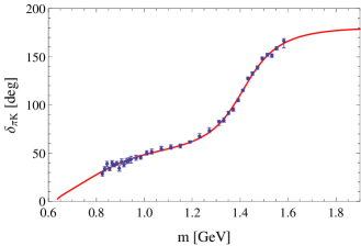
Figure 2: The solid (red) curve shows our fit result for the phase shift from Eq. (7) with respect to the four model parameters $a,b,\Lambda,m_{0}$ (see Table 1). The blue points are the data of Ref. Aston et al. (1988). A very good agreement is obtained.

By using the parameters listed in Table 1 we continue the propagator from Eq. (5) into the second Riemann sheet and scan the complex plane for poles. We find two poles (given in GeV) which we assign in the following way:

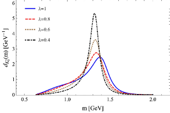
Figure 3: In the left panel we show the spectral function from Eq. (6) plotted for the parameters of Table 1. An enhancement for low values of the running mass $m$ is clearly visible. In the right panel we show the spectral function for different values of the scaling parameter $\lambda=3/N_{c}$. The smaller $\lambda$ is, the more peaked is the spectral function and the enhancement for low values of the running mass decreases.

$$K_{0}^{\ast}(1430) :\ (1.413\pm 0.002)-i\hskip 0.56917pt(0.127\pm 0.003)\ ,$$ (8)

$$K_{0}^{\ast}(800)\ :\ (0.746\pm 0.019)-i\hskip 0.56917pt(0.262\pm 0.014)\ .$$ (9)

Thus, a pole corresponding to the light $\kappa$ emerges very naturally in our calculation and is a dynamically generated state (for a discussion on the definition of dynamical generation, see Refs. Giacosa (2009); Guo and Oller (2015); Albaladejo and Oller (2012)). At this point, one should stress that the small errors quoted above (especially for what concerns the resonance $K_{0}^{\ast}(1430)$) are specific to our model defined in Eqs. (II), (2), and (4), respectively. In particular, the choice of the form factor (4) is model dependent, a fact that introduces an intrinsic uncertainty. We will explore this point in more detail in the next subsection, in which the positions of the poles are studied for different modifications of the model.

Table 1: Results of the fit. $\chi_{0}^{2}/d.o.f.=1.25$

Parameter	Value
$a$	$1.60\pm 0.22$ GeV
$b$	$-11.16\pm 0.82$ GeV-1
$\Lambda$	$0.496\pm 0.008$ GeV
$m_{0}$	$1.204\pm 0.008$ GeV

The PDG Olive et al. (2014) reports for $K_{0}^{\ast}(1430)$ a mass of $(1.425\pm 0.050)$ GeV and a width of $(0.270\pm 0.080)$ GeV. Our values fit very well in these windows. In particular, our width, obtained by doubling the negative imaginary part of our pole, reads $(0.254\pm 0.006)$ GeV and is thus determined with a small error. For $K_{0}^{\ast}(800)$ the PDG reports a mass of $(0.682\pm 0.029)$ GeV and a width of $(0.547\pm 0.024)$ GeV, which are also in agreement with our values (although our results point to a somewhat larger value for the mass). The mass $(0.746\pm 0.019)$ GeV and width $(0.524\pm 0.028)$ GeV determined within our model are also in good agreement with most of the pole determinations listed in Ref. Olive et al. (2014).

In the left panel of Fig. 3 we show the spectral function for the parameters of Table 1. A low-energy enhancement is present, but no peak. The absence of a peak is one of the reasons why the acceptance of the $\kappa$ might be considered to be controversial. However, if resonance poles on unphysical Riemann sheets are the relevant quantities, it turns out that the existence of the broad $\kappa$ is a consequence of our model.

Similar statements can be made concerning the broad isoscalar state $f_{0}(500)$: its pole is widely accepted while a clear peak in the spectral function is not present. On the contrary, the two scalar states $a_{0}(980)$ and $f_{0}(980)$ are pretty narrow: although their couplings are large, these resonances sit just at the kaon-kaon threshold, making their decays into kaons to be kinematically suppressed. In conclusion, all those states together with $\kappa$ seem to have their common origin in quantum fluctuations.

We also study the change of the spectral function and of the position of the poles when performing a rescaling of the coupling constants:

$$a\rightarrow\sqrt{\lambda}\hskip 0.56917pta,\ \ b\rightarrow\sqrt{\lambda}\hskip 0.56917ptb\ \ \ \text{with}\ \lambda\leq 1\ .$$ (10)

This is completely equivalent to a large-$N_{c}$ study upon setting

$$\lambda=\frac{3}{N_{c}}\ .$$ (11)

The spectral function is plotted in the right panel of Fig. 3 for different values of $\lambda$. Obviously, the low-energy enhancement becomes smaller for decreasing $\lambda$, $i.e.$, for increasing $N_{c}$.

Finally, we present the pole movement as function of $\lambda$ in Fig. 4. We observe that the pole of $K_{0}^{\ast}(1430)$ moves toward the real axis, a behavior expected for a quarkonium state.

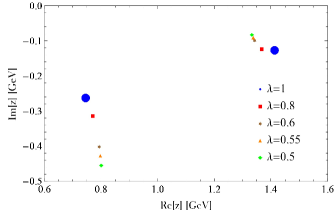
Figure 4: Movement of the two resonance poles for different values of $\lambda=3/N_{c}$. While the pole corresponding to $K_{0}^{\ast}(1430)$ moves toward the real axis, the pole of the light $K_{0}^{\ast}(800)$ moves away from the real axis and disappears for $\lambda\simeq 0.24$.

The pole of $K_{0}^{\ast}(800)$ moves away from the real axis and disappears for $\lambda\simeq 0.24$ (or $N_{c}\simeq 13$). From this it follows that the pole of $K_{0}^{\ast}(800)$ is dynamically generated and does not survive in the large-$N_{c}$ limit. Such a behavior was also reported in Refs. Zhou and Xiao (2011); Guo and Oller (2011); Guo et al. (2012); Peláez (2004b).

It should be stressed at this point that the choice of the form factor (4) is model dependent. A Gaussian form as implemented here is a standard choice when investigating mesonic resonances and the position of their poles, respectively, see also the discussion in Refs. Isgur and Speth (1996); *tornreply1; Harada et al. (1997); *harada2; Rupp et al. (2002). Yet, in Sec. III.2 we investigate possible variations of the form factor and indeed find that they are not capable of reproducing the phase shift data correctly. At the same time, we will also investigate the statistical significance of the fit presented in this subsection as well as the fits that we will discuss in Sec. III.2.

III.2 Variations of the model

In this subsection we investigate different scenarios in order to understand better how the results discussed in the previous part emerge. We first perform two fits to the phase shift data: one in which we consider only the non-derivative term in Eq. (II) (we set $b=0$), and one in which we consider only the derivative term (we set $a=0$).

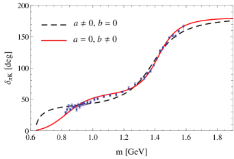
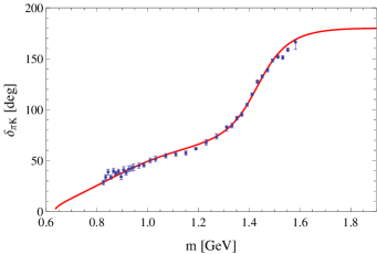
Figure 5: Left panel: The solid (red) and dashed (black) curves show our fit results for the phase shift from Eq. (7) with respect to the four model parameters $a,b,\Lambda,m_{0}$ (see Table 2). The blue points are the usual data of Ref. Aston et al. (1988). Right panel: The solid (red) curve shows the fit for the modified form factor in Eq. (13).

The results are presented in the left panel of Fig. 5 and in Table 2. The first entry summarizes what was found in the previous subsection. The second and third entries represent the two cases $b=0$ and $a=0$, respectively. As can be seen in the third column, in both cases the $\chi^{2}$ has increased, signalizing a worse agreement than with our first fit.

Table 2: Fitting results for the variations of the model.

Scenario	Parameters	$\chi_{0}^{2}/d.o.f.$	$p\left(\chi^{2}>\chi_{0}^{2}\right)$	Pole for $K_{0}^{\ast}(800)$	Pole for $K_{0}^{\ast}(1430)$
$a,b\neq 0$, Gaussian	$\!\begin{aligned} a&=1.60\pm 0.22\text{ GeV}\\ b&=-11.16\pm 0.82\text{ GeV}^{-1}\\ \Lambda&=0.496\pm 0.008\text{ GeV}\\ m_{0}&=1.204\pm 0.008\text{ GeV}\end{aligned}$	1.25	$0.15$	$\!\begin{aligned} (0.746\pm 0.019)\\ -i\hskip 0.56917pt(0.262\pm 0.014)\end{aligned}$	$\!\begin{aligned} (1.413\pm 0.002)\\ -i\hskip 0.56917pt(0.127\pm 0.003)\end{aligned}$
$b=0$, Gaussian	$\!\begin{aligned} a&=4.06\pm 0.04\text{ GeV}\\ \Lambda&=0.902\pm 0.015\text{ GeV}\\ m_{0}&=1.299\pm 0.002\text{ GeV}\end{aligned}$	5.41	$1.72\cdot 10^{-22}$	-	$\!\begin{aligned} (1.385\pm 0.002)\\ -i\hskip 0.56917pt(0.146\pm 0.003)\end{aligned}$
$a=0$, Gaussian	$\!\begin{aligned} b&=-17.10\pm 0.17\text{ GeV}^{-1}\\ \Lambda&=0.453\pm 0.002\text{ GeV}\\ m_{0}&=1.142\pm 0.002\text{ GeV}\end{aligned}$	2.54	$1.92\cdot 10^{-6}$	$\!\begin{aligned} (0.820\pm 0.003)\\ -i\hskip 0.56917pt(0.187\pm 0.002)\end{aligned}$	$\!\begin{aligned} (1.419\pm 0.001)\\ -i\hskip 0.56917pt(0.112\pm 0.002)\end{aligned}$
$a,b\neq 0$, $F_{\Lambda}(m)=e^{-2k^{4}(m)/\Lambda^{4}}$	$\!\begin{aligned} a&=2.32\pm 0.09\text{ GeV}\\ b&=-3.40\pm 0.26\text{ GeV}^{-1}\\ \Lambda&=0.652\pm 0.006\text{ GeV}\\ m_{0}&=1.248\pm 0.003\text{GeV}\end{aligned}$	2.86	$7.98\cdot 10^{-8}$	$\!\begin{aligned} (0.863\pm 0.008)\\ -i\hskip 0.56917pt(0.339\pm 0.017)\end{aligned}$	$\!\begin{aligned} (1.433\pm 0.002)\\ -i\hskip 0.56917pt(0.112\pm 0.003)\end{aligned}$

Yet, in order to be more quantitative, we report in the fourth column the results of a statistical test of the goodness of the fit: The quantity

$$p\left(\chi^{2}>\chi_{0}^{2}\right)=\frac{1}{2^{d/2}\Gamma(d/2)}\int_{\chi_{0}^{2}}^{\infty}\text{d}x\ x^{\frac{d}{2}-1}e^{-x/2}$$ (12)

(with $d=d.o.f.$) is the probability to obtain a larger value of the $\chi^{2}$ than $\chi_{0}^{2}$ if a new experiment shall be performed (by using, of course, the same theoretical function in the fit). When this probability is very small, one may conclude that $(i)$ the theoretical model is not correct (a reasonable conclusion) or $(ii)$ the theoretical model is correct but the experimental results show a – quite unlucky – statistical fluctuation. When this probability is, for instance, smaller than $5\%$, one can exclude the theoretical model at the $95\%$ confidence level. In our case, our preferred solution from the previous subsection gives $p\left(\chi^{2}>\chi_{0}^{2}\right)=15.3\%$, which implies that the theoretical model cannot be rejected (here, $d.o.f.=37-4=33$). On the contrary, the models with only non-derivative interactions and with derivative interactions can be rejected with a very high level of accuracy. While this result is expected for the non-derivative term because the shape of the theoretical function does not match the data (see left panel of Fig. 5), the situation is more subtle in the case of only derivative terms. Here, the form is by-eye qualitatively correct, but the statistical test shows that it is not in agreement with the experiment (with $d.o.f.=37-3=34$).

Finally, in the fifth and sixth columns we report for completeness the position of the poles for the various models. Yet, in view of the statistical analysis, only the first row can be regarded as reliable.

As a next step we investigate other types of the form factor. As explained before, the Gaussian form factor is rather standard in various works on the subject and it is also easy to use. Especially in presence of derivative interactions it is very practical since it cuts off the integrand in the loop integral sufficiently fast . However, there is no fundamental reason why the Gaussian should be the best one to apply. It is therefore important to check variations of it. We test the following simple modification:

$$F_{\Lambda}(m)=e^{-2k^{4}(m)/\Lambda^{4}}\ .$$ (13)

The result of the fit is reported in the right panel of Fig. 5 as well as in the last entry of Table 2. Also in this case, the right panel of Fig. 5 shows a qualitative agreement of the model with data. Yet, the statistical test excludes this model at a very high-level of accuracy. From this perspective it is not surprising to find the pole of the $\kappa$ to be not in agreement with our result in the previous subsection and with other listings in the PDG. Thus, changing the form factor does not guarantee a good description of data, especially for what concerns the $\kappa$.

We have also tried a Fermi function $F_{\Lambda}(m)=\big{[}(1+e^{-\alpha\Lambda^{2}})/(1+e^{\alpha(k^{2}(m)-\Lambda^{2})})\big{]}^{2}$ for various values of the parameter $\alpha.\$This form factor is approximately constant for small $k$ and rapidly decreases to zero for $k\sim\Lambda$ (the higher $\alpha$, the steeper the descent; for $\alpha\rightarrow\infty$ the Heaviside step-function is realized). But also for this choice it was not possible to obtain a fit which would pass the statistical test of the $\chi^{2}$.

In conclusion, our study confirms that the Gaussian form factor is an adequate choice for mesonic interactions, leading to results that are in a good agreement with the data up to $\sim 1.8$ GeV, when both a (dominant) derivative and a (subdominant) non-derivative interaction term are simultaneously taken into account.

IV Conclusions

The scalar sector of hadron physics has been in the center of debate both from the theoretical and experimental side since a long time. There seems to be a consensus nowadays that at least the scalar states below $1$ GeV are non-conventional mesons Amsler and Törnqvist (2004); *amslerrev2; Giacosa (2009). In particular, the role of hadronic loop contributions to the self-energy, such as the one in Fig. 1, has been found to be crucial in various studies Close and Törnqvist (2002); Peláez and Ríos (2006); *pelaez2; Peláez (2004b); Oller and Oset (1997); *oller2; *oller3; Oller and Oset (1999); Jamin et al. (2000); *oller6; van Beveren et al. (2006); Morgan and Pennington (1993); van Beveren et al. (1986); Törnqvist (1995); *tornqvist2; Boglione and Pennington (1997); *pennington; Giacosa and Pagliara (2007); *e38.

We have concentrated in this work on the channel $I=1/2$, $J=0$. Our model contains non-derivative and derivative interactions in agreement with effective approaches of low-energy QCD Gasser and Leutwyler (1984); *Ecker; *chpt2; Parganlija et al. (2013). It was demonstrated that, by using a single kaonic seed state, both scalar resonances $K_{0}^{\ast}(1430)$ and $K_{0}^{\ast}(800)$ (known as $\kappa$) can be described as complex propagator poles. The two poles are required in order to correctly reproduce phase shift data of $\pi K$ scattering. The spectral function of our model turns out to be not of the ordinary Breit–Wigner type, too, due to strong distortions in the low-energy regime, which are a direct consequence of the $\kappa$-pole.

In the large-$N_{c}$ limit this pole finally disappears; the corresponding state is therefore not a conventional quarkonium. On the contrary, the pole corresponding to $K_{0}^{\ast}(1430)$ approaches the real energy axis for large values of $N_{c}$, hence becomes very narrow, which is a general feature of a quark-antiquark state.

It must be stressed that the presence of derivative interactions is crucial for our results. They turn out to be the dominant contribution toward the description of the $\pi K$ phase shift. For the future, one should use more complete models than the one presented in this work. In particular, a model is desired which allows to study simultaneously the $I=1/2$ and the $I=3/2$ channels. For instance, the extended Linear Sigma Model of Ref. Parganlija et al. (2013), that was used here as a motivation for our Lagrangian with derivative and non-derivative terms, can be applied for this purpose. Preliminary results in this direction are encouraging: In the $I=1/2$ sector this more complete hadronic model reduces – also for what concerns the numerical values – to the Lagrangian of Eq. (II).