Pade spectroscopy of structural correlation functions: application to liquid gallium

Abstract

We propose the new method of fluid structure investigation which is based on numerical analytical continuation of structural correlation functions with Pade approximants. The method particularly allows extracting hidden structural features of non-ordered condensed matter systems from experimental diffraction data. The method has been applied to investigating the local order of liquid gallium which has non-trivial stricture in both the liquid and solid states. Processing the correlation functions obtained from molecular dynamic simulations, we show the method proposed reveals non-trivial structural features of liquid gallium such as the spectrum of length-scales and the existence of different types of local clusters in the liquid.

I Introduction

Gallium is a very specific metal Waseda et al. (1980). First of all, it has enormously large domain of its phase diagram corresponding to liquid state. For example, the temperature interval of stable liquid state at ambient pressure is $(302.93,2477)$ K. Diffraction experiments have shown that the local structure of liquid gallium is very complicated and it differs much from the local structure of typical simple liquids Narten (1972); Waseda and Suzuki (1972); Lyapin et al. (2008); Yagafarov et al. (2012). Accordingly, the crystal structure of gallium is also nontrivial: below its melting temperature $T_{m}=302.93$ at the ambient pressure the stable phase corresponds to the orthorhombic lattice which in nontypical for one-component metallic systems Wells (2012) (amount the other metals, the only Eu has the same lattice structure at ambient pressure). At higher pressures there is a lot of polymorphic transitions to other nontrivial crystal structures Schulte and Holzapfel (1997); Kenichi et al. (1998).

Last time a lot of theoretical efforts were concentrated on investigation of the local structures and anomalies of gallium in liquid phase Tsay and Wang (1994); Gong et al. (1993); Yang et al. (2011); Tsai et al. (2010). But there is a gap between theoretical investigations of gallium and experiment. The main problem is that the only way to directly access the local structure is performing molecular dynamic (MD) simulations which can not unambiguously describe structure of real materials. Indeed, classical MD deals with model approximate potentials and first-principles MD has a problem of restricted spatial and time scales available in simulations. Experiment also can not directly access the local structure: the information about angle correlations is mostly lost in the static structure factor or radial distribution function (RDF); so only radial correlations can be extracted. Here we develop a new method of correlation function processing based on complex analysis with Pade approximants.

Using this method we study local structure of liquid gallium and extract its non-trivial features. Analysing structural correlation functions obtained from MD simulations with EAM potentials, we extract the spectrum of spatial length scales and the existence of two types of local clusters. We show that the best fit of the gallium RDF can be performed using Lorentzians instead of Gaussians which are usually used for that purpose.

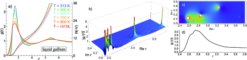
Figure 1: (Color online) Pade spectroscopy of radial distribution function. (a) Radial distribution function (RDF) $g(r)$ of liquid gallium (solid lines) and its cumulative function $N(<r)$ (dashed lines) at different temperatures $T$ (indicated on the plot). (b)-(d) Liquid gallium, $T=500$. (b) Doing the Pade approximation we find characteristic scales of gallium for particle distribution in the first coordination sphere: $r=2.58$, $r=2.69$, $r=2.84$. The scale $r=3.33$ corresponds to the tail of the first coordination sphere. (c) shows the density plot of the Pade approximant while (d) shows for comparison the first peak of $g(r)$.

II Local order of gallium

II.1 Methods

For MD simulations of liquid gallium, we have used $\rm{LAMMPS}$ molecular dynamics package. The system of $N=20000-100000$ particles interacting via EAM potential Belashchenko (2013), specially designed for gallium Belashchenko (2012), was simulated under periodic boundary conditions in Nose-Hoover NPT ensemble. This amount of particles is enough to obtain satisfactory results. More simulation details can be found in Ref. Mokshin et al. (2015) where similar simulation has been described. We checked that radial distribution functions obtained by our simulation quantitatively agree with those extracted from experiment Mokshin et al. (2015).

II.2 Local order: Pade spectroscopy of pair radial distribution

Figure 2: (Color online) RDF obtained for ideal lattice of $\alpha$-Ga with small random noise which mimics thermal vibrations. The cumulative function $N(<r)$ is also plotted by dashed line to evaluate the number of atoms at different shells.

Here we focus on gallium at ambient pressure and investigate how its properties in liquid state depend on temperature. Figure 1(a) shows the radial distribution function $g(r)$ of gallium taken for several temperatures in the range of $(313,1073)$ K. The cumulative function $N(<r)\equiv 4\pi\rho\int_{0}^{r}r^{\prime 2}g(r^{\prime})dr^{\prime}$, which is the mean number of particles inside a sphere of radius $r$, is also plotted in Fig. 1(a); in part, the cumulative function $N(<r)$ shows the number of nearest neighbors in the first coordination shell.

It is clear from the figure that the shape of the first RDF peak is nontrivial. It can be seen that the first RDF peak of gallium has clear shoulder. Particles forming the local clusters are mostly located at distances corresponding to the first coordination sphere (first peak of RDF). That suggests that local structure of liquid gallium is rather nontrivial. More detailed information can be extracted only after specific processing of RDF (see below).

The promising way to extract features of local order hidden in RDF is performing analytical continuation to complex plain of distances. This is usual way in the theory of correlation functions of quantum systems especially for analytical continuation of the Greens functions from imaginary (Matsubara Abrikosov et al. (1975)) frequencies to the real frequency domain Vidberg and Serene (1977); Yamada and Ikeda (2014); Schött et al. (2015). Recently the method of numerical analytical continuation was successfully applied to investigations of velocity autocorrelation function of Lennard-Jones fluid Krishnan and Ayappa (2003); Chtchelkatchev and Ryltsev (2015) and in classical hydrodynamics of the Stokes waves Dyachenko et al. (2014). Here we use this method, see Appendix A and Ref. Chtchelkatchev and Ryltsev (2015), for analysis of gallium RDFs.

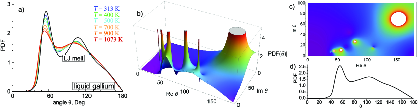
Figure 3: (Color online) Pade spectroscopy of bond angle distribution function (BADF). (a) BADF of liquid gallium at different temperatures $T$ (indicated on the plot). Additionally the BADF of LJ melt (which is nearly universal on the LJ melting curve) is also plotted for the comparison. (b-d) show BADF for $T=500$ and its processing with Pade approximant. We see a number of poles, their positions ($\operatorname{Re}\theta$) give characteristic angles between the particles forming local order clusters.

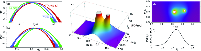
Figure 4: (Color online) Pade spectroscopy of probability distribution functions (PDF). (a) and (b) show orientational local order of liquid gallium: PDFs of the bond order parameters $q_{l}$ ($l$ = 4, 6) taken at two temperatures $T\--$ 313 K (blue line) and 1073 K (red line). Green solid lines represent the same PDFs for the LJ melt taken on the melting line (it can be shown that along the melting line these PDFs are practically universal KlumovPrivateComm). (c) and (d) show the absolute value of PDF ($l=6$) of gallium for $T=500$ in complex $q_{6}$-plain. (e) is PDF of gallium for $T=500$ plotted for comparison with poles of the PADE-approximant in (d). The poles are situated at $\operatorname{Re}q_{6}=0.32,\,0.42$.

The static structure factor is related to RDF as Hansen and McDonald (2013):

$$S(k)=1+\frac{4\pi}{\rho}\operatorname{Im}\int_{0}^{\infty}r(g(r)-1)e^{ikr}dr.$$ (1)

So, if $g(r)$ has a pole, at the position $r_{p}$, we should expect that the contribution of this pole to the structure factor oscillates like $\cos(k\operatorname{Re}r_{p})$ or $\sin(k\operatorname{Re}r_{p})$ and decays with $k$ like $e^{-k\operatorname{Im}r_{p}}$. Thus, knowledge of the poles gives important scales characterising the particle system.

In Figs. 1(b) and (c) we show the results of the typical processing of gallium RDF by Pade approximants. As follows we use Pade approximant of RDF for its analytical continuation in complex-$r$. Fig. 1(b) shows the absolute value of RDF in complex-$r$ plain while the peaks correspond to the poles. We see a limited number of poles near the real axis: so the Lorenzian fit of RDF perfectly matches all its basic features, see Figs. 1(c) and (d). The real parts of the positions of the poles are important length scales characterising gallium: as follows, in the first coordination sphere: $r=2.58$, $r=2.69$, $r=2.84$; the scale $r=3.33$ corresponds to the tail of the first coordination sphere. These scales are in fact characteristic interparticle distances in the first coordination shell. Thus we see that analytical continuation with Pade approximants allows extracting multi-scale character of local structure of liquid gallium. In that connection, remember that, at ambient pressure, gallium crystallizes into non-trivial orthorhombic lattice and so it is interesting to find relation between unusual multiscale local order of the liquid and non-trivial crystal symmetry.

In Fig.2 we show RDF obtained for ideal lattice of $\alpha$-Ga (orthorhombic) with small random noise which mimics thermal vibrations. We see that first coordination shell contains two atoms located at short distance of 2.46 ${\AA}$. Such ${\rm Ga_{2}}$ dimers were earlier suggested to be formed by covalent-like bonding Gong et al. (1991). Each Ga atom has another six nearest neighbour located in pairs in different coordination shells at distances $2.7$, $2.73$, $2.79$ ${\AA}$. So the crystal structure of $\alpha$-Ga demonstrates spectrum of spatial scales. The comparison of these scales with those obtained from analytical continuation of RDF shows good agreement. Indeed the ratios of maximal and minimal distances are $1.134$ for experimental lattice structure and $1.1$ for scales extracted from liquid RDF. Of course the analytical continuation of liquid RDF does not distinct two nearly located scales. Recently, the similar analysis of liquid Ga structure was performed in Mokshin et al. (2015) where simulated RDF were approximated by a set of Gaussians that gave similar interval of spatial scales. However this methods can distinct only two scales in mentioned interval. Moreover the results strongly depend on the choice of approximation parameters such as the number and the shape of approximating functions.

II.3 Local order: Pade spectroscopy of orientational order

More detailed structural information can be obtained from analysis of orientational local order. The simplest way to describe it is calculating angular distribution function $P(\theta)$ which is probability density of angle $\theta$ between two vectors connecting a particle with its two nearest neighbors.

Fig. 3 shows bond angle distribution functions of liquid gallium at different temperatures $T$ (indicated on the plot). Additionally the BADF of LJ-melt (which is nearly universal on the LJ melting curve) is also plotted for the comparison. Figure 3(b-d) show BADF for $T=500$. Looking at BADFs at real-$\theta$ axis, it is difficult to say something specific about the clusters forming the local order. But after its processing with the Pade approximant we see a number of poles in complex-$\theta$ plain. The positions of poles ($\operatorname{Re}\theta$) give characteristic angles between the particles forming the local order clusters. Particulary, we see two pronounced poles at the vicinity of the first peak which are located near the angles $45$ and $60$. The value of $\theta=60$ is typical for simple liquids and corresponds to tetrahedral local order Ryltsev and Chtchelkatchev (2013). But the angle $\theta=45$ suggests non-trivial symmetry of local clusters probably caused by the existence of short-bonded particles revealed by RDF analysis.

Another way to analyse orientational order is the well known bond order parameter method, which is widely used to characterize order in simple fluids, solids and glasses Steinhardt et al. (1983, 1981); R. (2003); Rein ten Wolde et al. (1996); Klumov (2013); Fomin et al. (2014) hard spheres D. (1996); Klumov et al. (2011), colloidal suspensions Gasser et al. (2001), complex plasmas Rubin-Zuzic et al. (2006); Klumov (2010); Khrapak et al. (2011) and metallic glasses Hirata et al. (2013).

Basic description of bond order distribution functions (BODF) can be found in Appendix B. To quantify the local orientational order, it is also convenient to use the probability distribution functions (PDFs) $P(q_{l})$ and $P(w_{l})$. Figure 4 shows the PDFs at different $l$ ($l=4,~{}6$) at different temperatures of liquid gallium in comparison to those calculated for LJ liquid whose PDFs are nearly universal along the melting line KlumovPrivateComm. We se again that such PDFs calculated at real-$q_{l}$ axis (Fig. 4a,b) reveal no interesting features of liquid gallium structure. We see broad dome-shaped distributions which are similar to those for LJ liquids. But analytical continuation in the complex-$q$ plane reveals that $P(q_{l})$ are in fact composed of two Lorenzian-like peaks with similar values of both the maximum location (${\rm Re}(q)$) and peak width (${\rm Im}(q)$). This fact suggests the structure of liquid gallium consists of two types of local order that is in agreement with the earlier obtained results Yagafarov et al. (2012); Yang et al. (2011).

III Discussion

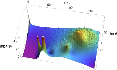
Figure 5: (Color online) Stability test of PDF analytical continuation shown in Fig. 3(b).

There is important question related to the accuracy of numerical analytical continuation and stability of poles to errors in the initial data. We solve this problem doing two procedures.

We build the Pade-approximant on top known function values $f(x_{i})=u_{i}$ in the discrete set of points $x_{i}$ on the real axis, see Appendix A. We always randomly shuffle the set of points $x_{i}$ using the Fisher–Yates–Knuth shuffle algorithm Knuth (1997) before building the Pade continued fraction approximant. Then we average the approximant over a considerable number of shuffles. This procedure helps avoiding specific errors related to numerical calculation of long continued-fraction.

Next, the accuracy of the Pade extrapolation of the function depends on the distribution of points $x_{i}$: maximum accuracy corresponds to the uniform distribution of $x_{i}$. Doing the stability test we randomly take away about 10$\%$ of points $x_{i}$: this procedure makes the distribution of $x_{i}$ nonuniform and moves the “unstable” poles in the complex plain if there are any. Finally we build the extrapolation $\tilde{f}$ of the function $f$ averaging the Pade approximant over $10000$ random extractions of initial points $x_{i}$. Then when we draw $|\tilde{f}(z)|$ at complex $z$, unstable poles disappear while the poles suffering from the insufficient accuracy of $f(x_{i})$ average into “domes”.

This procedure is illustrated in Fig. 5. We test here PDF shown in Fig. 3(b) using the procedure described above. Poles at $\operatorname{Re}\theta\approx 44$ and $\operatorname{Re}\theta\approx 57$ are stable. The other poles shown in Fig. 3(b) are not wrong, but their positions are more sensitive to the accuracy of the PDF-table. So after each random taking away some of the knots $\theta_{i}$, the positions of the poles slightly change and finally after 10000 such procedures we see domes at the positions where in Fig. 3(b) we have seen poles. This test show that we can trust all the pole except, probably, one situated at $\operatorname{Re}\theta\approx 79$. (More refined stability test however shows that even this pole should not be completely disregarded.)

This procedure is illustrated in Fig. 5. We test here PDF shown in Fig. 3(b) using the method described above. Poles at $\operatorname{Re}\theta\approx 44$ and $\operatorname{Re}\theta\approx 57$ are stable. The other poles shown in Fig. 3(b) are not wrong, but their positions are more sensitive to the accuracy of the PDF-table. So after each random taking away some of the knots $\theta_{i}$, the positions of the poles slightly change and finally after averaging over 10000 such extractions we see domes at the positions where in Fig. 3(b) we have seen poles. This test shows that we can trust all the poles except, probably, one situated at $\operatorname{Re}\theta\approx 79$. (More refined stability test however shows that even this pole should not be completely disregarded.) The coordinates of the “dome” top in the complex plain we should take then as the characteristic parameters. If we compare them with the coordinates of the poles in Fig. 3(b) we will see coincidence with the satisfactory accuracy.

IV Conclusions

We propose the new method of fluid structure investigation which is based on numerical analytical continuation of structural data obtained from both experiment and computer simulations. The method particularly allows extracting hidden structural features of non-ordered condensed matter systems from experimental diffraction data. The method has been applied to investigating the local order of liquid gallium which is supposed to have complex stricture. We show that analytical continuation of structural correlation functions such as radial distribution function, bond angle distribution function and bond orientational order parameters reveals non-trivial structural features of liquid. Firstly, we show that, processing the liquid RDF, our method allows easily obtaining the spectrum of length-scales which are in close agreement with those for crystal state. Secondly, we show for the first time that correlation functions of orientational order also have non-trivial features probably caused by the existence of different types of local clusters in the liquid.

We also show that the best fit of the radial distribution function can be performed using Lorentzians instead of Gaussians which are usually used for that purpose.

Appendix A Pade approximants method

Here we discuss the construction of the Padé approximants that interpolate a function given $N$ knot points. Pade-approximants are the rational functions (ratio of two polinomials). A rational function can be represented by a continued fraction. Typically the continued fraction expansion for a given function approximates the function better than its series expansion. Here we use “multipoint” algorithm Vidberg and Serene (1977); Baker and Graves-Morris (1996); wol to build the Pade-approximant. Suppose we know function values $f(x_{i})=u_{i}$ in the discrete set of points $x_{i}$ where the “knots” $x_{i}$, $i=1,2,3,\ldots,N$. Then the Pade approximant

$$C_{N}(x)=\frac{a_{1}}{\frac{a_{2}\left(x-x_{1}\right)}{\frac{a_{3}\left(x-x_{2}\right)}{\frac{a_{4}\left(x-x_{3}\right)}{\ldots a_{N}\left(x-x_{N-1}\right)+1}+1}+1}+1}$$ (2)

where $a_{i}$ we determine using the condition, $C_{N}(x_{i})=u_{i}$, which is fulfilled if $a_{i}$ satisfy the recursion relation

$$a_{i}=g_{i}\left(x_{i}\right),\qquad g_{1}\left(x_{i}\right)=u_{i},\qquad i=1,2,3,\ldots,N.$$ (3)

$$g_{p}(x)=\frac{g_{p-1}(x_{p-1})-g_{p-1}(x)}{\left(x-x_{p-1}\right)g_{p-1}(x)},\qquad p\geq 2.$$ (4)

Eq. (3) is the “boundary condition” for the recursive relation Eq. (4). For example, taking $x=x_{i_{0}}$ we get $g_{1}(x_{i})$ from (3) and $g_{j}(x_{i_{0}})$, $j=2,3,\ldots,i$ from (4). Accuracy of the analytical continuation can be tested by permutations of $x_{i}$ and/or by the random extraction of some part of the knots and permutation averaging.

Appendix B Bond orientational order analysis

Table 1: Bond order parameters $q_{l}$ and $w_{l}$ ($l=4,~{}6$) calculated via the fixed number of nearest neighbors (NN) for a few crystalline structures and cumulants of the corresponding BODF for the LJ melt

. lattice type  $q_{4}$  $q_{6}$  $w_{4}$  $w_{6}$ hcp (12 NN) 0.097 0.485 0.134 -0.012 fcc (12 NN) 0.19 0.575 -0.159 -0.013 ico (12 NN) $1.4\times 10^{-4}$ 0.663 -0.159 -0.169 bcc ( 8 NN) 0.5 0.628 -0.159 0.013 bcc (14 NN) 0.036 0.51 0.159 0.013 LJ melt (12 NN) $\approx$0.155 $\approx$0.37 $\approx$-0.023 $\approx$-0.04

Each particle $i$ is connected via vectors (bonds) with its $N_{\rm nn}(i)$ nearest neighbors (NN), and the rotational invariants (RIs) of rank $l$ of second $q_{l}(i)$ and third $w_{l}(i)$ orders are calculated as:

$$q_{l}(i)=\left({4\pi\over(2l+1)}\sum_{m=-l}^{m=l}|~{}q_{lm}(i)|^{2}\right)^{1/2}$$ (5)

$$w_{l}(i)=\sum\limits_{\begin{array}[]{cc}{}_{m_{1},m_{2},m_{3}}\\ {}_{m_{1}+m_{2}+m_{3}=0}\end{array}}\left[\begin{array}[]{ccc}l&l&l\\ m_{1}&m_{2}&m_{3}\end{array}\right]q_{lm_{1}}(i)q_{lm_{2}}(i)q_{lm_{3}}(i),$$ (6)

where $q_{lm}(i)=N_{\rm nn}(i)^{-1}\sum_{j=1}^{N_{\rm nn}(i)}Y_{lm}({\bf r}_{ij})$, $Y_{lm}$ are the spherical harmonics and ${\bf r}_{ij}={\bf r}_{i}-{\bf r}_{j}$ are vectors connecting centers of particles $i$ and $j$. In Eq.(6), $\left[\begin{array}[]{ccc}l&l&l\\ m_{1}&m_{2}&m_{3}\end{array}\right]$ are the Wigner 3$j$-symbols, and the summations performed over all the indexes $m_{i}=-l,...,l$ satisfying the condition $m_{1}+m_{2}+m_{3}=0$. As shown in the pioneer paperSteinhardt et al. (1983), the bond order parameters $q_{l}$ and $w_{l}$ can be used as measures to characterize the local orientational order and the phase state of considered systems.

Because each lattice type has a unique set of bond order parameters, the method of RIs can be also used to identify lattice and liquid structures in mixed systems. The values of $q_{l}$ and $w_{l}$ for a few common lattice types (including liquid-like Lennard-Jones melt) are presented in Table 1.

References

- Waseda et al. (1980) Y. Waseda et al., The structure of non-crystalline materials: liquids and amorphous solids (McGraw-Hill New York, 1980).
- Narten (1972) A. H. Narten, J. Chem. Phys. 56 (1972).
- Waseda and Suzuki (1972) Y. Waseda and K. Suzuki, Phys. Status Solidi B 49, 339 (1972).
- Lyapin et al. (2008) A. Lyapin, E. Gromnitskaya, O. Yagafarov, O. Stal gorova, and V. Brazhkin, JETP 107, 818 (2008).
- Yagafarov et al. (2012) O. F. Yagafarov, Y. Katayama, V. V. Brazhkin, A. G. Lyapin, and H. Saitoh, Phys. Rev. B 86, 174103 (2012).
- Wells (2012) A. F. Wells, Structural inorganic chemistry (Oxford University Press, 2012).
- Schulte and Holzapfel (1997) O. Schulte and W. B. Holzapfel, Phys. Rev. B 55, 8122 (1997).
- Kenichi et al. (1998) T. Kenichi, K. Kazuaki, and A. Masao, Phys. Rev. B 58, 2482 (1998).
- Tsay and Wang (1994) S.-F. Tsay and S. Wang, Phys. Rev. B 50, 108 (1994).
- Gong et al. (1993) X. G. Gong, G. L. Chiarotti, M. Parrinello, and E. Tosatti, Europhys. Lett. 21, 469 (1993).
- Yang et al. (2011) J. Yang, J. S. Tse, and T. Iitaka, J. Chem. Phys. 135, 044507 (2011).
- Tsai et al. (2010) K. H. Tsai, T.-M. Wu, and S.-F. Tsay, J. Chem. Phys. 132, 034502 (2010).
- Belashchenko (2013) D. K. Belashchenko, Physics-Uspekhi 56, 1176 (2013).
- Belashchenko (2012) D. Belashchenko, Russian Journal of Physical Chemistry A 86, 779 (2012).
- Mokshin et al. (2015) A. Mokshin, R. Khusnutdinoff, A. Novikov, N. Blagoveshensky, and A. Puchkov, JETP 148, 947 (2015).
- Abrikosov et al. (1975) A. A. Abrikosov, L. P. Gorkov, and I. E. Dzyaloshinski, Methods of quantum field theory in statistical physics (Courier Corporation, 1975).
- Vidberg and Serene (1977) H. Vidberg and J. Serene, J. Low Temp. Phys. 29, 179 (1977).
- Yamada and Ikeda (2014) H. Yamada and K. Ikeda, European Physical Journal B 87, 1 (2014).
- Schött et al. (2015) J. Schött, I. L. Locht, E. Lundin, O. Grånäs, O. Eriksson, and I. Marco, arXiv preprint arXiv:1511.03496 (2015).
- Krishnan and Ayappa (2003) S. H. Krishnan and K. G. Ayappa, J. Chem. Phys. 118, 690 (2003).
- Chtchelkatchev and Ryltsev (2015) N. Chtchelkatchev and R. Ryltsev, Pis ma v ZhETF 102, 732 (2015).
- Dyachenko et al. (2014) S. Dyachenko, P. Lushnikov, and A. Korotkevich, JETP Letters 98, 675 (2014).
- Hansen and McDonald (2013) J.-P. Hansen and I. R. McDonald, Theory of Simple Liquids: With Applications to Soft Matter (Academic Press, 2013).
- Gong et al. (1991) X. G. Gong, G. L. Chiarotti, M. Parrinello, and E. Tosatti, Phys. Rev. B 43, 14277 (1991).
- Ryltsev and Chtchelkatchev (2013) R. E. Ryltsev and N. M. Chtchelkatchev, Phys. Rev. E 88, 052101 (2013).
- Steinhardt et al. (1983) P. J. Steinhardt, D. R. Nelson, and M. Ronchetti, Phys. Rev. B 28, 784 (1983).
- Steinhardt et al. (1981) P. J. Steinhardt, D. R. Nelson, and M. Ronchetti, Phys. Rev. Lett. 47, 1297 (1981).
- R. (2003) E. J. R., J. Chem. Phys. 118, 2256 (2003).
- Rein ten Wolde et al. (1996) P. Rein ten Wolde, M. J. Ruiz-Montero, and D. Frenkel, J. Chem. Phys. 104 (1996).
- Klumov (2013) B. Klumov, JETP Letters 97, 327 (2013).
- Fomin et al. (2014) Y. D. Fomin, V. N. Ryzhov, B. A. Klumov, and E. N. Tsiok, J. Chem. Phys. 141, 034508 (2014).
- D. (1996) R. M. D., J. Chem. Phys. 105, 9258 (1996).
- Klumov et al. (2011) B. A. Klumov, S. A. Khrapak, and G. E. Morfill, Phys. Rev. B 83, 184105 (2011).
- Gasser et al. (2001) U. Gasser, E. R. Weeks, A. Schofield, P. N. Pusey, and D. A. Weitz, Science 292, 258 (2001).
- Rubin-Zuzic et al. (2006) M. Rubin-Zuzic et al., Nature Phys. 2, 181 (2006).
- Klumov (2010) B. A. Klumov, Physics-Uspekhi 53, 1053 (2010).
- Khrapak et al. (2011) S. A. Khrapak, B. A. Klumov, P. Huber, V. I. Molotkov, A. M. Lipaev, V. N. Naumkin, H. M. Thomas, A. V. Ivlev, G. E. Morfill, O. F. Petrov, V. E. Fortov, Y. Malentschenko, and S. Volkov, Physical Review Letters 106, 205001 (2011).
- Hirata et al. (2013) A. Hirata, L. J. Kang, T. Fujita, B. Klumov, K. Matsue, M. Kotani, A. R. Yavari, and M. W. Chen, Science 341, 376 (2013).
- Knuth (1997) D. E. Knuth, The Art of Computer Programming, Volume 2 (3rd Ed.): Seminumerical Algorithms (Addison-Wesley Longman Publishing Co., Inc., Boston, MA, USA, 1997).
- Baker and Graves-Morris (1996) G. A. Baker and P. R. Graves-Morris, Padé Approximants, Vol. 59 (Cambridge University Press, 1996).
- (41) Multipoint Padé Approximants (Wolfram Mathworld).