Coqblin-Schrieffer Model for an Ultra-cold Gas of Ytterbium atoms with Metastable States

Abstract

Motivated by the impressive recent advance in manipulating cold ytterbium atoms we explore and substantiate the feasibility of realizing the Coqblin-Schrieffer model in a gas of cold fermionic ¹⁷³Yb atoms. Making use of different AC polarizabillity of the electronic ground state (electronic configuration ¹S₀) and the long lived metastable state (electronic configuration ³P₀), it is substantiated that the latter can be localized and serve as a magnetic impurity while the former remains itinerant. The exchange mechanism between the itinerant ¹S₀ and the localized ³P₀ atoms is analyzed and shown to be antiferromagnetic. The ensuing SU(6) symmetric Coqblin-Schrieffer Hamiltonian is constructed, and, using the calculated exchange constant $J$, perturbative renormalization group (RG) analysis yields the Kondo temperature $T_{K}$ that is experimentally accessible. A number of thermodynamic measurable observables are calculated in the weak coupling regime $T>T_{K}$ (using perturbative RG analysis) and in the strong coupling regime $T<T_{K}$ (employing known Bethe ansatz techniques).

I Introduction

Ever since its discovery, the physics exposed in cold atom systems proves to be a godsend for elucidating spectacular physical phenomena that are otherwise extremely difficult to access elsewhere CAGen ; CAFerm ; UCA-pra04 ; UCA-Adv-At-Mol-Opt-Phys06 ; UCA-pra06 ; UCA-nucl-phys07 ; UCA-Varena06 ; UCA-nature08 ; UCA-IntJModPhys09 ; UCA-Nature10 ; UCA-Science10 ; ExpExc-nature10 ; Exp-exch-Science08 ; exch-arxiv-15-07 ; exch-prl-15 ; exch-nature-15 ; Nature03 ; arXiv09 ; prb09 ; NaturePhys09 ; Greiner-PhD-03 . Special attention is recently focused on quantum magnetism in general, and impurity problems in particular KE-UCA-prl-10 ; KE-UCA-arxiv-15-07 ; KE-UCA-arxiv-15-02 ; 2CKECA ; Dem ; opt-latt-11 ; Demler-Salomon ; ITYK . One of the reasons is that a cold atom system opens a way to study the physical properties of a gas of fermionic atoms with half-integer spin $s\geq\frac{3}{2}$, thereby enabling the study of novel impurity problems. The main goal of this paper is to develop this general idea into an experimental and theoretical framework wherein the Coqblin-Schrieffer model can be realized in an atomic gas of cold ¹⁷³Yb atoms.

In the “traditional” Kondo effect Kondo-64 ; Coleman-PhysWorld-95 ; Anderson-PhysWorld-95 ; Hewson-book , a magnetic impurity of spin ${\mathbf{S}}$ immersed in a metal host, scatters the itinerant electrons having spin ${\mathbf{s}}$ ($s=\frac{1}{2}$) through an antiferromagnetic exchange interaction $J{\mathbf{s}}\cdot{\mathbf{S}}$ with $J>0$, and the pertinent dynamics is governed by the $s$-$d$ exchange Hamiltonian Hewson-book . In the Coqblin-Schrieffer model Hewson-book ; Rajan-prl-83 ; Schlottmann-83 ; KE-prb-98 ; Coq-Schr-arxiv-01 ; Coq-Schr-prb-03 ; Coq-Schr-JPhSocJpn-07 ; KA-prb14 ; Coq-Schr-Physica14 , the itinerant fermions and the impurity are both $N$-fold “spin” degenerate, so that the corresponding Hamiltonian has an SU($N$) symmetry. The main difference between the s-d exchange model for spin $S=\tfrac{1}{2}$ and the Coqblin-Schrieffer model for “spin” $S>\frac{1}{2}$ is that, due to exchange scattering, the change of the $z$-component of the angular momentum of the impurity is restricted to $0,\pm 1$ in the s-d model, while it is unrestricted in the Coqblin-Schrieffer model. In solid state physics, the high level degeneracy is due to spin-orbit coupling, so that the model is relevant for applications to rare earth impurities. In a gas of ultracold atoms, the degeneracy is due solely to the atomic total angular momentum ${\bf F}={\bf I}+{\bf J}$, where ${\bf I}$ is the nuclear spin and ${\bf J}$ is the total (orbital and spin) electronic angular momentum.

Realizing the Coqblin-Schrieffer model in cold fermionic ¹⁷³Yb atoms is feasible due to a rather unique exchange mechanism. The atoms in the ¹S₀ ground-state form a Fermi gas with SU($N$) symmetry and the atoms in the long-lived ³P₀ excited state assume the role of localized magnetic impurities. Both the ground and excited states have spin $F=\frac{5}{2}$ (which is the nuclear spin). The idea is to localize an excited ³P₀ atom in a state-dependent optical potential, such that it will serve as a magnetic impurity, immersed in a Fermi gas of ground state ¹S₀ atoms. The latter is confined in a combination of harmonic and periodic potentials but otherwise are itinerant. We show that an antiferromagnetic exchange interaction exists between the itinerant and localized atoms and that the ensuing exchange scattering is described by the Coqblin-Schrieffer Hamiltonian.

In Sec. II we briefly review the advantage of using degenerate alkaline-earth-like atoms such as Yb and Sr for the study the Kondo effect and its SU($N$) extension in cold atom experiments. Then, in Sec. III, we present a general description of the system composed of a mixture of ¹⁷³Yb atoms in their ground and excited states. Atomic quantum states in the optical potential are described in Subsec. III.1, while the exchange interaction between Yb atoms in the ground and excited states is derived in Subsec. III.2. This exchange interaction is somewhat unusual because it occurs between the same atoms whose electronic angular momentum is zero. In Subsec. III.3 we derive the SU($N$) Kondo Hamiltonian and estimate the Kondo temperature. Calculations of observables are detailed in Sec. IV, and naturally divided into the weak and strong coupling regimes. The magnetic susceptibility, entropy and specific heat of the impurity, in the weak coupling regime (${T}>{T}_{K}$) are estimated in Subsection IV.1. Magnetic susceptibility, entropy and specific heat of the impurity in the strong coupling regime ($T<T_{K}$) are derived in Subsecsection IV.2. Our main results are summarized in Sec. V. Details of the derivation of the exchange interaction between two Yb atoms in ¹S₀ and ³P₀ respective atomic states are expanded upon in the Appendix. It is shown and underlined there that precise calculation of the exchange constant requires a detailed knowledge of the atomic wave functions. Although these details are of technical nature, they expose how the exchange interaction determines the scattering length, and demonstrate the extreme sensitivity of the relation between the singlet and triplet scattering lengths on the one hand and the magnitude of the exchange interaction on the other hand. Indirect exchange interaction is considered in subsection A.1. It is shown that the exchange is antiferromagnetic. This conclusion does not depend on a chosen model or an approximation but is general property of the second order perturbation theory. Wave function describing motion of interacting atoms is derived in subsection A.2. We derive here expression for the scattering length. In subsection A.3 we compare our results for the scattering length with experimental results of Ref. 6 . In subsection A.4 we study confinement-induced resonances (CIR) where the exchange interaction changes from ferromagnetic to antiferromagnetic and vise versa.

II Kondo effect with cold alkaline atoms

Recent advance in the techniques of cooling and manipulating degenerate alkaline-earth-like atoms (e.g. ytterbium and/or strontium atoms) 1 ; 2 ; 3 paves the way for studying novel aspects of interacting Fermi systems. These include non-equilibrium properties such as transport, as well as impurity problems and other facets of quantum magnetism. A key role in these considerations is played by the interplay between the long-lived metastable ³P₀ state and the ¹S₀ ground state, with their enlarged SU($N$) spin symmetry for fermionic isotopes add1 ; add2 . Utilizing a narrow singlet-triplet optical transition, for example, alkaline-earth-like atoms have been thought of as a promising candidate for realizing a precise atomic clock add3 or ideal storage of qubits for the application of quantum computing add2 .

Here we consider the possible occurrence of the Kondo effect and its SU($N$) extensions in a gas of ytterbium atoms. Making use of different AC polarizabilities of the ground-state (¹S₀) and the long lived metastable (³P₀) state, the localized ³P₀ atoms can serve as magnetic impurities which interact with itinerant ground-state atoms 4 ; 4-1 ; 4-2 . The Kondo effect arises when this interaction is characterized by spin-exchange between ¹S₀ and ³P₀ state. Such spin-exchange interactions has recently been demonstrated5 ; 6 ; 7 in fermionic ¹⁷³Yb atoms.

Realizing the Kondo effect in alkali-earth-like atoms exposes novel aspects of the Kondo physics with SU($N$) symmetric interactions that are difficult to elucidate in solid-state based system, because the high SU($N$) symmetry arises from the strong decoupling between nuclear and electronic spins in alkali-earth-like atoms. As such, it has attracted much interest in the context of SU($N$) Fermi gases both for bulk systems 8 ; 9 ; 10 and for lattice systems 11 . Here, we focus on the SU($N$) Kondo model in the fermionic ¹⁷³Yb gas, and estimate the Kondo temperature. In cold atom systems, due to the weak magnetic coupling of spin-exchange interactions, the questions still remains whether or not the Kondo temperature is attainable by current experiments. Our finding shows that the Kondo temperature is enhanced by the SU($N$) interactions. In electronic systems, this is shown in previous works on heavy fermion systems Hewson-book ; Coleman and on carbon nanotube quantum dots KA-prb14 . Indeed, the Kondo temperature in cold atom system may also be enhanced by means of the confinement-induced resonance 11 or by the orbital-induced Feshbach resonance 12 ; 13 ; 14 ; SU3-KE-cold-atoms-PRL13 .

III Description of the System

Having underlined the peculiar advantage of using alkaline atoms to explore the Kondo effect and its SU($N$) extensions, we now focus a cold gas of ¹⁷³Yb fermionic atoms confined in a shallow harmonic potential. Most of the atoms remain in the ground state ¹S₀ and form a Fermi sea due to its half integer nuclear spin $I=\tfrac{5}{2}$ (purple area in Fig. 1). However, a few atoms are found in a long lived excited ³P₀ state following a coherent excitation via the clock transition. These excited atoms can be trapped in a state-dependent optical lattice potential as schematically displayed in Fig. 1 (red circles), and can be regarded as localized impurities. The wavelength of the periodic optical potential exceeds the range of interaction between atoms, thereby justifying the assumption that the concentration of excited atoms is small enough so that they are not correlated.

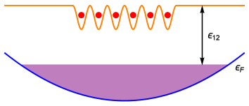
Figure 1: Illustration of a “Kondo model” for ¹⁷³Yb atoms. Atoms in the ground-state ¹S₀ form a Fermi sea, while atoms in the excited-state ³P₀ are trapped in an optical potential and form a dilute concentration of localized magnetic impurities (see details in the text).

In the following, we describe such mixture of ¹⁷³Yb atomic system within a model of uncorrelated and localized magnetic impurities. To this end, the details of an exchange interaction between an atom in the ground-state and an atom in an excited state is of crucial importance. Since both atoms in the ground and excited states are in an electronic singlet state, direct exchange interaction between these atoms is absent. There is, however, an indirect exchange, that involves virtual hopping of electrons between the atoms such that an atom transforms from the ground state to an excited state, whereas the other atom transforms from an excited state to the ground state. An expression for this exchange interaction is derived below, followed by an analysis of the corresponding impurity problem, that turns out to be a manifestation of the Coqblin-Schrieffer model realized in cold atom systems.

III.1 Quantum States of ¹⁷³Yb Atoms with van der Waals Interaction

Before discussing exchange interaction between two Yb atoms it is important to analize the single atom properties because the exchange interaction is crucially dependent on the electronic wave functions of a single atom. An ¹⁷³Yb atom can be considered as a charged (+2) closed shell rigid ion and two valence electrons. The ground-state ¹S₀ valence electrons configuration is $6s^{2}$, while that of the excited state ³P₀ is 6$s$6$p$. The excitation energy $\epsilon_{12}=\epsilon_{2}-\epsilon_{1}$ is spectral-line-Yb

$$\epsilon_{12} = 2.14349~{}{\mathrm{eV}}.$$

The positions of the ion core and the outer electrons are respectively specified by vectors $\mathbf{R}$, $\mathbf{r}_{\mathrm{a}}$ and $\mathbf{r}_{\mathrm{b}}$ (Fig. 2).

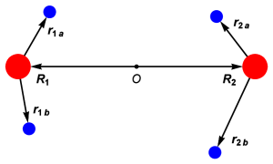
Figure 2: Two ytterbium atoms. The position of the rigid ions are $\mathbf{R}_{1}$ and $\mathbf{R}_{2}$, positions of the electrons are ${\bf{r}}_{1{\mathrm{a}}}$, ${\bf{r}}_{1{\mathrm{b}}}$, ${\bf{r}}_{2{\mathrm{a}}}$ and ${\bf{r}}_{2{\mathrm{b}}}$. The origin of the frame is denoted as $O$.

The ytterbium atoms are trapped by state-dependent trapping potentials $V_{\mathrm{g},\mathrm{e}}(\mathbf{R})$,

$$V_{\mathrm{g}}(\mathbf{R}) = V_{\mathrm{g}}^{(0)}k_{\mathrm{g}}^{2}R^{2},\ \ \ R~{}=~{}|\mathbf{R}|,$$ (1)

$$V_{\mathrm{e}}(\mathbf{R}) = V_{\mathrm{e}}^{(0)}\sum_{i}\sin^{2}\big{(}k_{\mathrm{e}}X_{i}\big{)},$$ (2)

where $i$ is a Cartesian index. The potential parameters are tuned such that

$$V_{\mathrm{g}}^{(0)}k_{\mathrm{g}}^{2}~{}\ll~{}V_{\mathrm{e}}^{(0)}k_{\mathrm{e}}^{2},$$ (3)

and therefore the atoms in the ground state are considered as itinerant atoms, and the atom in the excited state plays a role of the impurity.

In the adiabatic (Born-Oppenheimer) approximation (which is well substantiated in atomic physics), the wave function of a single ytterbium atom is expressed as a product of the wave functions $\Psi(\mathbf{R})$ (for the rigid ion core) and $\psi(\mathbf{r}_{a},\mathbf{r}_{b})$ (for the valence electrons). The former is considered as a point particle of mass $M$ whose position vector in Cartesian coordinates is ${\bf R}=(X,Y,Z)$.

Starting with the core wave functions, recall that the atoms in the ground-state and the excited state are subject to different 3D optical potentials and van der Waals interactions between the atoms. Strictly speaking, we should describe the system by many-particle wave function $\Psi(\mathbf{R}_{0};\{\mathbf{R}\}_{\cal{N}})$, where ${\cal{N}}$ is the number of itinerant atoms, $\{\mathbf{R}\}_{\cal{N}}=\{\mathbf{R}_{1},\mathbf{R}_{2},\ldots,\mathbf{R}_{\cal{N}}\}$, $\mathbf{R}_{j}$ is the position of an itinerant atom ($j=1,2,\ldots,{\cal{N}}$) and $\mathbf{R}_{0}$ is the position of the impurity atom. When the distance between all the atoms exceeds the range of the vad der Waals interaction, the many-particle wave function splits into a product of single-particle wave functions. When an itinerant atom is placed close to the impurity and all other atoms are far away, the many particle wave function is a product of a two-particle wave function describing interacting pair of atoms, and single particle wave functions describing motion of the other itinerant atoms. Usually, the density of itinerant atoms is low and the probability to find two or more itinerant atoms close to the impurity is negligible small. Therefore, we can describe the many atomic system in terms of two-atomic wave functions. For this purpose we use the notations $\Psi(\mathbf{R}_{1},\mathbf{R}_{2})$ for the core wave functions pertaining for two atoms in the ground or excited electronic states. They are solutions of the following Schrödinger equation:

$${\cal{H}}\Psi(\mathbf{R}_{1},\mathbf{R}_{2}) = {\cal{E}}\Psi(\mathbf{R}_{1},\mathbf{R}_{2}).$$ (4)

Here $\mathbf{R}_{1}$ is the position of the atom in the ground state, $\mathbf{R}_{2}$ is the position of the atom in the excited state. The two particle Hamiltonian ${\cal{H}}$ is,

$${\cal{H}} = {\cal{H}}_{\mathrm{g}}+{\cal{H}}_{\mathrm{e}}+W\big{(}|\mathbf{R}_{1}-\mathbf{R}_{2}|\big{)}.$$ (5)

The first or second terms on the right hand side of eq. (5) describe motion of the atom in the groung or excited state,

$${\cal{H}}_{\mathrm{g}} = -\frac{\hbar^{2}}{2M}~{}\frac{\partial^{2}}{\partial\mathbf{R}_{1}^{2}}+V_{\mathrm{g}}(\mathbf{R}_{1}),$$ (6)

$${\cal{H}}_{\mathrm{e}} = -\frac{\hbar^{2}}{2M}~{}\frac{\partial^{2}}{\partial\mathbf{R}_{2}^{2}}+V_{\mathrm{e}}(\mathbf{R}_{2}),$$ (7)

where $M$ is the atomic mass. Recall that the trapping potentials $V_{\mathrm{g},\mathrm{e}}(\mathbf{R})$ are defined in Eqs. (1) and (2).

The third term on the right hand side of eq. (5) is the Van der Waals interaction between the ytterbium atoms. Explicitly, it is expressed as, vdW-Yb-PRA-08 ; vdW-Yb-PRA-14

$$W(R) = \frac{C_{6}}{R^{6}}~{}\bigg{\{}\frac{\sigma^{6}}{R^{6}}-1\bigg{\}}-\frac{C_{8}}{R^{8}}.$$ (8)

Here $C_{6}=2.651\cdot 10^{3}E_{h}a_{B}^{6}$, $C_{8}=3.23640441\cdot 10^{5}E_{h}a_{B}^{8}$ and $\sigma=9.0109361a_{B}$, where $E_{h}=27.211$ eV is the Hartree energy and $a_{B}=0.52918$ Å is the Bohr radius.

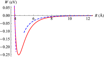
Figure 3: Van der Waals interatomic interaction (solid red curve), its approximation by $-C_{6}/R^{6}$ (blue dashed curve) and linear approximation near the classical turning point $R=r_{0}$ (dashed purple line).

Van der Waals potential is illustrated in Fig. 3. It is equal to zero when $R=r_{0}$, where $r_{0}=3.9$ Å. At $R=a_{0}=4.4$ Å, the potential $W(R)$ reaches its minimum, $W(a_{0})=-0.25$ eV.

III.1.1 Wave Function at Long Distances between the Atoms

There is a characteristic length $\lambda$ associated with the van der Waals potential,

$$\lambda = \bigg{(}\frac{MC_{6}}{\hbar^{2}}\bigg{)}^{1/4}~{}=~{}89.97~{}{\text{\AA}}.$$ (9)

When the distance between the atoms exceeds $\lambda$, we can neglect the van der Waals interaction. In this case the two atomic wave function $\Psi(\mathbf{R}_{1},\mathbf{R}_{2})$ takes the form of a product of two single atomic wave functions, $\Psi_{\mathrm{g}}(\mathbf{R}_{1})$ and $\Psi_{\mathrm{e}}(\mathbf{R}_{2})$,

$$\Psi(\mathbf{R}_{1},\mathbf{R}_{2}) = \Psi_{\mathrm{g}}(\mathbf{R}_{1})\Psi_{\mathrm{e}}(\mathbf{R}_{2}).$$

The wave functions $\Psi_{\mathrm{g},\mathrm{e}}(\mathbf{R})$ are respectively the eigenfunctions of the Hamiltonians ${\cal{H}}_{\mathrm{g}}$ and ${\cal{H}}_{\mathrm{e}}$, that is,

$$-\frac{\hbar^{2}}{2M}~{}\frac{\partial^{2}\Psi_{\mathrm{g},\mathrm{e}}(\mathbf{R})}{\partial\mathbf{R}^{2}}+V_{\mathrm{g},\mathrm{e}}(\mathbf{R})\Psi_{\mathrm{g},\mathrm{e}}(\mathbf{R})=\varepsilon\Psi_{\mathrm{g},\mathrm{e}}(\mathbf{R}).$$ (10)

Consider first the wave function $\Psi_{\mathrm{e}}(\mathbf{R})$. When the corresponding energy level $\varepsilon_{\mathrm{imp}}$ is deep enough, the wave function of the bound state near the potential minimum at $\mathbf{R}=0$ can be approximated within the harmonic potential picture as

$$\Psi_{\mathrm{e}}(\mathbf{R}) = \frac{1}{\big{(}\pi b_{\mathrm{e}}^{2}\big{)}^{3/4}}~{}\exp\bigg{(}-\frac{R^{2}}{2b_{\mathrm{e}}^{2}}\bigg{)},$$ (11)

where the harmonic length and frequency are

$$k_{\mathrm{e}}b_{\mathrm{e}}=\bigg{[}\frac{\hbar^{2}k_{\mathrm{e}}^{2}}{2MV_{\mathrm{e}}^{(0)}}\bigg{]}^{1/4},\ \ \Omega_{\mathrm{e}}=\sqrt{\frac{2V_{\mathrm{e}}^{(0)}k_{\mathrm{e}}^{2}}{M}}.$$ (12)

Energy level of the impurity is

$$\varepsilon_{\mathrm{imp}}=\frac{3\hbar\Omega_{\mathrm{e}}}{2}.$$ (13)

Next, consider the wave functions $\Psi_{\mathrm{g}}(\mathbf{R})$ of the ytterbium atom in the ground state for which the shallow potential wells are not deep enough to form tightly bound states. Hence, we can neglect the “fast” potential relief and take into account just isotropic potential $V_{\mathrm{g}}(\mathbf{R})$. Quantum states of atoms in isotropic potential (1) are described by the radial quantum number $n$ [$n=0,1,2,\ldots$], orbital quantum number $L$ [$L=0,1,2,\ldots$] and projection $m$ of the orbital moment on the axis $z$ [$m=-L,-L+1,\ldots,L$]. Due to the centrifugal barrier, only the atoms with $L=0$ can approach the impurity and be involved in the exchange interaction with it. The wave functions of the states with $L=0$ found from the Schrödinger equation (10) are,

$$\Psi_{\mathrm{g}}^{n}(\mathbf{R})={\cal{N}}_{n}~{}L_{n}^{(\frac{1}{2})}\bigg{(}\frac{R^{2}}{b_{\mathrm{g}}^{2}}\bigg{)}\exp\bigg{(}-\frac{R^{2}}{2b_{\mathrm{g}}^{2}}\bigg{)},$$ (14)

where $L_{n}^{(l+\frac{1}{2})}(\varrho)$ are generalized Laguerre polynomials. The normalization factor is:

$${\cal{N}}_{n}~{}=~{}\bigg{(}\frac{1}{2\pi b_{\mathrm{g}}^{2}}\bigg{)}^{3/4}~{}\sqrt{\frac{2^{n+2}~{}n!}{(2n+1)!!}}.$$

The harmonic length $b_{\mathrm{g}}$ and frequency $\Omega_{\mathrm{g}}$ are defined through,

$$k_{\mathrm{g}}b_{\mathrm{g}}~{}=~{}\bigg{(}\frac{\hbar^{2}k_{\mathrm{g}}^{2}}{2MV_{\mathrm{g}}^{(0)}}\bigg{)}^{1/4},\ \ \ \Omega_{\mathrm{g}}~{}=~{}\sqrt{\frac{2V_{\mathrm{g}}^{(0)}k_{\mathrm{g}}^{2}}{M}}.$$ (15)

The corresponding energy levels are

$$\varepsilon_{n} = \hbar\Omega_{\mathrm{g}}\bigg{(}2n+\frac{3}{2}\bigg{)}.$$ (16)

The inequality (3) imply

$$\Omega_{\mathrm{g}}~{}\ll~{}\Omega_{\mathrm{e}}.$$

Within this framework, the spectrum is nearly continuous and the ytterbium atoms in the ground-state form a Fermi gas. The Fermi energy $\epsilon_{F}$ is such that $\epsilon_{F}\gg\hbar\Omega_{\mathrm{g}}$, hence the Fermi gas is 3D.

III.1.2 Wave Function at Short Distances between the Atoms

In order to elucidate the behavior of the two atomic wave function within the interval $|\mathbf{R}_{1}-\mathbf{R}_{2}|\lesssim\lambda$, we adopt the semiclassical technique developed in Ref. Scatt-Length-WKB-PRA93 : Introduce the coordinate $\mathbf{R}_{c}$ of the center of mass and the relative coordinate $\mathbf{R}$,

$$\mathbf{R}_{c}~{}=~{}\frac{1}{2}~{}\big{(}\mathbf{R}_{1}+\mathbf{R}_{2}\big{)},\ \ \ \ \ \mathbf{R}~{}=~{}\mathbf{R}_{1}-\mathbf{R}_{2}.$$ (17)

In the next step, we take into account that the van der Waals potential (8) has an effective range $\lambda$, Eq. (9), and therefore $|\mathbf{R}|\lesssim\lambda$. Employing the following inequalities,

$$k_{\mathrm{g}}\lambda~{}\ll~{}k_{\mathrm{e}}\lambda~{}\ll~{}1,$$

we can write

$$V_{\mathrm{e}}\bigg{(}\mathbf{R}_{c}-\frac{\mathbf{R}}{2}\bigg{)} = V_{\mathrm{e}}\big{(}\mathbf{R}_{c}\big{)}+O\big{(}k_{\mathrm{e}}\lambda\big{)},$$

$$V_{\mathrm{g}}\bigg{(}\mathbf{R}_{c}+\frac{\mathbf{R}}{2}\bigg{)} = V_{\mathrm{g}}^{(0)}~{}k_{\mathrm{g}}^{2}R_{c}^{2}.$$

The motion of the atom in the excited state is restricted within the area $|\mathbf{R}_{2}|\approx|\mathbf{R}_{c}|\lesssim b_{\mathrm{e}}$. Taking into account the inequality $k_{\mathrm{g}}b_{\mathrm{e}}\ll 1$, we can neglect $V_{\mathrm{g}}(R)$ within the intervals,

$$\big{|}\mathbf{R}_{2}\big{|}~{}\lesssim~{}b_{\mathrm{e}},\ \ \ \ \ \big{|}\mathbf{R}_{1}-\mathbf{R}_{2}\big{|}~{}\lesssim~{}\lambda.$$

Then the two atomic wave function is a product of two functions, $\Psi_{c}(\mathbf{R}_{c})$ and $\Psi_{r}(\mathbf{R})$, which satisfy the equations,

$$\bigg{\{}-\frac{\hbar^{2}}{4M}~{}\frac{\partial^{2}}{\partial\mathbf{R}_{c}^{2}}+V_{\mathrm{e}}\big{(}\mathbf{R}_{c}\big{)}\bigg{\}}\Psi_{c}(\mathbf{R}_{c})={\cal{E}}_{c}\Psi_{c}(\mathbf{R}_{c}),$$ (18)

$$\bigg{\{}-\frac{\hbar^{2}}{M}~{}\frac{\partial^{2}}{\partial\mathbf{R}^{2}}+W(R)\bigg{\}}\Psi_{r}(\mathbf{R})={\cal{E}}_{r}~{}\Psi_{r}(\mathbf{R}).~{}~{}~{}~{}~{}$$ (19)

Effect of the trapping potential $V_{\mathrm{e}}(\mathbf{R}_{2})$ on the relative motion of the atoms is considered in Appendix A.4. Eq. (18) yields the wave function of a bound state near the minimum of $V_{\mathrm{e}}(\mathbf{R})$ at $\mathbf{R}=0$. Before analyzing the wave-function $\Psi_{r}(\mathbf{R})$, we note that the total energy of the two atom system is

$${\cal{E}}_{n}~{}=~{}{\cal{E}}_{c}+{\cal{E}}_{r}.$$

On the other side, this same quantity is also given as:

$${\cal{E}}_{n}~{}=~{}\varepsilon_{\mathrm{imp}}+\varepsilon_{n},$$

where $\varepsilon_{n}$ is given by eq. (16). For the degenerate Fermi gas, $\varepsilon_{n}\leq\epsilon_{F}$ and $\hbar\Omega_{\mathrm{e}}<\epsilon_{F}$. Usually the Fermi energy $\epsilon_{F}$ is such that the Fermi temperature $T_{F}=\epsilon_{F}/k_{B}$ lies within the interval [see Ref. 5 , for example]

$$T_{F}~{}<~{}300~{}{\text{nK}}.$$

The depth of the van der Waals potential is $W(a_{0})=0.25$ eV [see Fig. 3]. Then we can neglect ${\cal{E}}_{r}\sim\varepsilon_{n}$ with respect to the van der Waals potential (8) at the distances $R\lesssim\lambda$. Then the Schrödinger equation (19) takes the form,

$$\bigg{\{}-\frac{\hbar^{2}}{M}~{}\frac{\partial^{2}}{\partial\mathbf{R}^{2}}+W(R)\bigg{\}}~{}\Psi_{r}\big{(}\mathbf{R}\big{)}~{}=~{}0.$$ (20)

The potential $W(R)$ depends just on the distance $R$ from the impurity. Therefore, the orbital momentum $L$ and its projection $m$ on the axis $z$ are good quantum numbers. Because of the centrifugal barrier, just atoms with $L=0$ can approach close one to another. Therefore we restrict ourselves by considering just the s-wave (i.e., the wave with $L=0$). Solution of the equation (20) is evident but rather cumbersome [see Ref. Scatt-Length-WKB-PRA93 and subsection A.2 for details]. The wave function of the s-wave satisfying eq. (20) is

$$\Psi_{n}(\mathbf{R}) = \frac{\psi_{n}(R)}{\sqrt{4\pi}~{}R},$$ (21)

where $n$ is the harmonic quantum number defined by eq. (16). In order to find the radial wave function $\psi_{n}(R)$, it is useful to employ different approximations in several corresponding intervals as defined below. To this end, we underline the following constraints on the parameters $R$: $r_{0}$, $b_{0}$ and $\lambda$ as follows:

• $r_{0}$ is determined from the equation $W(r_{0})=0$. The classical mechanics allows motion of the zero-energy particle in the interval $R>r_{0}$.

• $b_{0}$ is constrained by the inequality,

  $$\bigg{|}\frac{\sigma^{6}}{b_{0}^{6}}-\frac{C_{8}}{C_{6}b_{0}^{2}}\bigg{|}~{}\ll~{}1.$$

  For ${R}\geq{b}_{0}$, we can approximate $W(R)\approx-C_{6}/R^{6}$. Practically, we take $b_{0}\approx 10$ Å [see Fig. 3].

• $\lambda=(MC_{6}/\hbar^{2})^{1/4}=89.97$ Å. In principle, the Wentzel-Kramers-Brillouin (WKB) approximation can be used for for $R\ll\lambda$.

A brief list of approximations per intervals is as follows (see details below): For the interval $r_{0}<R\ll\lambda$, we can apply the WKB approximation to solve the Schrödinger equation (19). For the interval $b_{0}<R<\lambda$, we can approximate $W(R)$ by $-C_{6}/R^{6}$ and solve eq. (19). The interval $R<r_{0}$ corresponds to classically forbidden region where the wave function decays exponentially. In the following discussions, we find the wave function within each interval. The intervals $r_{0}<R\ll\lambda$ and $b_{0}<R<\lambda$ overlap one with another since there is a wide interval $b_{0}<R\ll\lambda$ where both the WKB approximation and the approximation $W(R)\approx-C_{6}/R^{6}$ are valid. Therefore, within this interval both the approaches should give the same solution. We use this condition as as a connection condition for the solutions within two overlapping intervals.

1. Interval $r_{0}<R\ll\lambda$: The wave function calculated within the WKB approximation with quantum corrections Scatt-Length-WKB-PRA93 ; vdW-Yb-PRA-08 is,

$$\psi_{n}^{(1)}(R) = \frac{A_{1n}}{\sqrt{K(R)}}~{}\sin\Big{(}\Phi_{r}(R)+\frac{\pi}{4}\Big{)}.$$ (22)

where

$$\Phi_{r}(R) = \int\limits_{r_{0}}^{R}K(R^{\prime})dR^{\prime},$$ (23)

$$K(R) = \frac{1}{\hbar}~{}\sqrt{-MW(R)}.$$ (24)

When the distance between the atoms exceeds $\lambda$, the interaction between the atoms can be neglected and the two-atomic wave function is a product of the single-atomic wave functions (11) and (14). The wave function $\psi_{n}(R)$ and its derivative $\psi^{\prime}_{n}(R)$ are continues at $R=\lambda$. These conditions give

$$A_{1n} = \frac{2~{}\sqrt{k_{n}\lambda}}{\pi a_{\mathrm{g}}}~{}\Gamma\bigg{(}\frac{3}{4}\bigg{)}~{}\sqrt{1+\Big{(}\frac{a_{w}-\bar{a}}{\bar{a}}\Big{)}^{2}},$$ (25)

where

$$k_{n}~{}=~{}\frac{2\sqrt{n}}{a_{\mathrm{g}}},$$ (26)

the parameters $a_{w}$ and $\bar{a}$ are given by Eqs. (32) and (33) below.

2. Interval $R>b_{0}$: Within this interval, we can approximate the potential energy by $W(R)\approx-C_{6}/R^{6}$. The wave function $\psi_{n}^{(2)}(R)$ fir this interval is,

$$\psi_{n}^{(2)}(R) = A_{2n}~{}\tilde{\psi}_{2A}(R)+B_{2n}~{}\tilde{\psi}_{2B}(R),$$ (27)

where $\tilde{\psi}_{2A}(R)$ and $\tilde{\psi}_{2B}(R)$ are,

$$\tilde{\psi}_{2A}(R) = \sqrt{\frac{2R}{\lambda}}~{}J_{1/4}\bigg{(}\frac{\lambda^{2}}{2R^{2}}\bigg{)},$$ (28a)

$$\tilde{\psi}_{2B}(R) = \sqrt{\frac{2R}{\lambda}}~{}J_{-1/4}\bigg{(}\frac{\lambda^{2}}{2R^{2}}\bigg{)}.$$ (28b)

There is a large interval $b_{0}<R\ll\lambda$, where we can approximate $W(R)$ by $-C_{6}/R^{6}$ and apply the WKB approximation Scatt-Length-WKB-PRA93 . Therefore, we can apply the following connection conditions: For any $R$ within the interval $b_{0}<R\ll\lambda$, the equality $\psi_{n}^{(1)}(R)=\psi_{n}^{(2)}(R)$ is valid. This conditions gives,

$$A_{2n} = -A_{1n}~{}\frac{\sqrt{\pi\lambda}}{2}~{}\cos\Big{(}\Phi_{w}+\frac{\pi}{8}\Big{)},$$ (29a)

$$B_{2n} = A_{1n}~{}\frac{\sqrt{\pi\lambda}}{2}~{}\sin\Big{(}\Phi_{w}+\frac{3\pi}{8}\Big{)},$$ (29b)

where

$$\Phi_{w} = \int\limits_{r_{0}}^{\infty}K(R)~{}dR.$$ (30)

Figure 4: Wave functions $\tilde{\psi}_{2A}(R)$ and $\tilde{\psi}_{2B}(R)$, eq. (28) [solid curves] and their asymptotic (31) [dashed lines].

The functions $\tilde{\psi}_{2A}(R)$ and $\tilde{\psi}_{2B}(R)$, eq. (28) are shown in Fig. 4, solid lines. It is seen that for $R>\lambda$, the functions $\tilde{\psi}_{2A}(R)$ and $\tilde{\psi}_{2B}(R)$ are well approximated by the linear with $R$ expressions shown by dashed lined. Explicitly, the asymptotic expressions for $\tilde{\psi}_{2A}(R)$ and $\tilde{\psi}_{2B}(R)$ are,

$$\tilde{\psi}_{2A}(R)=\frac{1}{\Gamma(5/4)}~{}\Bigg{\{}1-\frac{\lambda^{4}}{20R^{4}}+O\bigg{(}\frac{\lambda^{8}}{R^{8}}\bigg{)}\Bigg{\}},$$ (31a)

$$\tilde{\psi}_{2B}(R)=\frac{2R/\lambda}{\Gamma(3/4)}~{}\Bigg{\{}1-\frac{\lambda^{4}}{12R^{4}}+O\bigg{(}\frac{\lambda^{8}}{R^{8}}\bigg{)}\Bigg{\}}.$$ (31b)

Eqs. (27) and (31) show that the asymptote of the wave function $\psi_{n}^{(2)}(R)$ at $R\gtrsim\lambda$ is $\psi_{n}^{(2)}(R)\propto{R-a_{w}}$, with the scattering length $a_{w}$ being Scatt-Length-WKB-PRA93 ; vdW-Yb-PRA-08 ,

$$a_{w} = \bar{a}~{}\bigg{\{}1-\tan\Big{(}\Phi_{w}-\frac{\pi}{8}\Big{)}\bigg{\}},$$ (32)

where

$$\bar{a} = \frac{\lambda}{2^{3/2}}~{}\frac{\Gamma\big{(}\frac{3}{4}\big{)}}{\Gamma\big{(}\frac{5}{4}\big{)}}~{}=~{}43.01~{}{\text{\AA}}.$$ (33)

For the potential (8), $\Phi_{w}=294.273$ and

$$a_{w} = 650.6~{}{\text{\AA}}.$$ (34)

III.2 Exchange Interaction

The strength of the exchange interaction between Yb(¹S₀) and Yb(³P₀) atoms,

$$J = -\frac{4\pi\hbar^{2}\big{(}a_{S}-a_{T}\big{)}}{M},$$ (35)

in which $a_{S}$ and $a_{T}$ are the singlet and triplet scattering lengths. The exchange interaction is ferromagnetic (antiferromagnetic) when $a_{S}-a_{T}$ is positive (negative). It is crucial to note that the fact that the Yb(³P₀) is trapped (while the Yb(¹S₀) is itinerant affects the value of $J$. The effect of trapping of the Yb(³P₀) impurity on the scattering lengths is calculated in the Appendix A.4. It is shown there that for free Yb atoms, $a_{S}>a_{T}$, and the exchange interaction is ferromagnetic. On the other hand, localization of the Yb(³P₀) atom can modify the scattering lengths and leads to confinement-induced resonances (CIR), which change the exchange interaction from ferromagnetic to antiferromagnetic and vise versa [see Fig. 11 for illustration].

III.3 Kondo Hamiltonian and the Kondo Temperature

Due to centrifugal barrier, only atoms with $L=0$ interact with the impurity. Omitting the states with nonzero $L$, we write the Hamiltonian of the system as

$$H=H_{0}+H_{K},$$ (36)

where

$$H_{0}~{}=~{}\sum_{n\mu}\varepsilon_{n}c_{n\mu}^{{\dagger}}c_{n\mu},$$ (37)

$$H_{K}~{}=~{}J\sum_{nn^{\prime}}\Psi_{\mathrm{g}}^{n}(0)\Psi_{\mathrm{g}}^{n^{\prime}}(0)\sum_{\mu}Z^{\mu\mu}c_{n^{\prime}\mu}^{{\dagger}}c_{n\mu}+$$

$$~{}~{}~{}~{}~{}~{}~{}+J\sum_{nn^{\prime}}\Psi_{\mathrm{g}}^{n}(0)\Psi_{\mathrm{g}}^{n^{\prime}}(0)\sum_{\mu\neq\mu^{\prime}}X^{\mu\mu^{\prime}}c_{n^{\prime}\mu^{\prime}}^{{\dagger}}c_{n\mu}.$$ (38)

Here $c_{n\mu}$ ($c_{n\mu}^{{\dagger}}$) is the annihilation (creation) operator for an atom of the Fermi gas, with harmonic quantum number $n$ and nuclear spin quantum number $\mu=-\tfrac{5}{2},-\tfrac{3}{2},\ldots,\tfrac{5}{2}$. $X^{\mu\mu^{\prime}}=|\mu\rangle\langle\mu^{\prime}|$ are the Hubbard operators coupling different degenerate impurity states, and

$$Z^{\mu\mu} = X^{\mu\mu}-\frac{1}{N}\sum_{\mu^{\prime}}X^{\mu^{\prime}\mu^{\prime}},\ \ \ \ \ N=6.$$

The density of states for the Hamiltonian $H_{0}$ is,

$$\rho(\epsilon) = \sum_{n}\Big{|}\Psi_{\mathrm{g}}^{n}(0)\Big{|}^{2}\delta(\epsilon-\varepsilon_{n})$$ (39)

$$\approx \frac{1}{b_{\mathrm{e}}^{3}}~{}\frac{\sqrt{\epsilon}}{\big{(}2\hbar\Omega_{\mathrm{e}}\big{)}^{3/2}}~{}\Theta(\epsilon),$$

where $\Theta(\epsilon)$ is the Heaviside theta function.

Within poor man scaling formalism, the dimensionless coupling $j=J\rho(\epsilon_{F})$ satisfies the following scaling equation Hewson-book :

$$\frac{\partial j}{\partial\ln D} = -Nj^{2}.$$ (40)

Initially, the bandwidth is $D_{0}=T_{\mathrm{e}}$,

$$T_{\mathrm{e}}=\frac{\hbar\Omega_{\mathrm{e}}}{k_{B}},$$

and the reduced bandwidth $D$ satisfies the inequalities ${D_{0}}\geq{D}\gg{T}$. The initial value of $j(D)$, $j(D_{0})\equiv{j}_{0}$ is,

$$j_{0} = \frac{J_{0}}{b_{\mathrm{e}}^{3}}~{}\frac{\sqrt{\epsilon_{F}}}{\big{(}2\hbar\Omega_{\mathrm{e}}\big{)}^{2}}$$ (41)

$$= -\frac{\pi\big{(}a_{S}-a_{T}\big{)}}{b_{\mathrm{e}}}~{}\sqrt{\frac{2\epsilon_{F}}{\hbar\Omega_{\mathrm{e}}}}.$$

Eq. (41) shows that the KE exists when $a_{S}<a_{T}$. Scattering lengths for free Yb(¹S₀) and Yb(³P₀) atoms are Scazza-Yb-3P0-2015 $a_{S}=\big{(}1878\pm 37\big{)}~{}a_{B}$ and $a_{T}=\big{(}219.7\pm 2.2\big{)}~{}a_{B}$, and the exchange interaction is ferromagnetic. The situation is changed when Yb(³P₀) atom is trapped. When the ground-state energy of the two atoms is equal to an energy of the trapped molecule, a confinement-induced resonance (CIR) occurs CIR-PhysRevLett-2003 ; CIR-PhysRevLett-2010 ; CIR-PhysRevLett-2005 ; CIR-PhysRevA-2006 . In this case, the exchange interaction changes from ferromagnetic to antiferromagnetic. CIR is considered in Appendix A.4. It is shown that for

$$1692a_{B}<b_{\mathrm{e}}<1819a_{B},$$ (42)

$a_{S}<0$, and the exchange interaction is antiferromagnetic, whereas for

$$212.8a_{B}<b_{\mathrm{e}}<226.7a_{B},$$ (43)

$a_{T}$ is positive and very large, and the exchange interaction is antiferromagnetic.

The scaling equation (40) has the solution,

$$j(T) = \frac{1}{N\ln\big{(}T/T_{K}\big{)}},$$ (44)

where the Kondo temperature (the scaling invariant of the RG equation) is given by

$$T_{K} = D_{0}\exp\bigg{(}-\frac{1}{Nj_{0}}\bigg{)}.$$ (45)

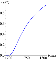
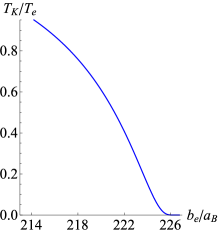
Figure 5: Kondo temperature (45) as a function of $T_{\mathrm{e}}$ for $D_{0}=T_{F}=T_{\mathrm{e}}$ and $b_{\mathrm{e}}$ belonging to (a) the interval (42) and (b) the interval (43).

The Kondo temperature (45) as a function of $T_{\mathrm{e}}$ is shown in Fig. 5 for $D_{0}=T_{F}=T_{\mathrm{e}}$ (purple curves). It is seen that $T_{K}$ is large enough and can be measured in experiment.

IV Calculation of Observables

Having set up the model and the corresponding Coqblin-Schrieffer Hamiltonian, it is then possible to predict experimentally measurable observables. At this stage we are content with presenting a few thermodynamics quantities appropriate for a system in thermal equilibrium. These include the impurity contributions to the magnetic susceptibility, specific heat and entropy. Calculations in the weak coupling regime $T>T_{K}$ require different techniques than those in the strong coupling regime, hence they are presented separately. Specifically, in the weak coupling regime one applies the RG formalism, while in the strong coupling regime the Bethe Ansatz (BA) analyses is employed. Both techniques are well documented and the resulting quantities are universal functions of $T/T_{K}$. Since we have already estimated $T_{K}$, we can use the known universal expressions for computing and presenting the pertinent thermodynamic quantities.

IV.1 Magnetic Susceptibility, specific heat and entropy in the Weak Coupling Regime

Since the ytterbium atoms are in a quantum state where the total electronic angular momentum is zero, the only contribution to magnetism is due to the nucleus (the nuclear spin is $5/2$).
Magnetization: The impurity contribution to the magnetization is defined through the relation Hewson-book ,

$${\mathbf{M}}_{\mathrm{imp}} = g_{\mathrm{Yb}}\mu_{\mathrm{n}}\Big{\{}\big{\langle}{\mathbf{S}}+{\mathbf{s}}\big{\rangle}-\big{\langle}{\mathbf{s}}\big{\rangle}_{0}\Big{\}},$$ (46)

where $\langle\cdots\rangle$ indicates thermal averaging with respect to the full Hamiltonian $H$, whereas $\langle\cdots\rangle_{0}$ indicates thermal averaging respect to $H_{0}$. $g_{\mathrm{Yb}}=-0.2592$ is the nuclear g-factor of ¹⁷³Yb nuclear-moment , and $\mu_{\mathrm{n}}$ is the nuclear magneton,

$$\mu_{\mathrm{n}} = \frac{e\hbar}{2m_{\mathrm{p}}c},$$

where $m_{\mathrm{p}}$ is the proton rest mass, and $c$ is the speed of light. ${\mathbf{S}}$ and ${\mathbf{s}}$ are the nuclear spin operators for the impurity and the itinerant atoms, explicitly written as

$${\mathbf{S}}~{}=~{}\sum_{\mu\mu^{\prime}}{\mathbf{t}}_{\mu\mu^{\prime}}X^{\mu\mu^{\prime}},$$

$${\mathbf{s}}~{}=~{}\sum_{{\mathbf{nn}}^{\prime}\mu\mu^{\prime}}{\mathbf{t}}_{\mu\mu^{\prime}}c_{{\mathbf{n}}\mu}^{{\dagger}}c_{{\mathbf{n}}^{\prime}\mu^{\prime}},$$

where $\hat{\mathbf{t}}=(\hat{t}^{x},\hat{t}^{y},\hat{t}^{z})$ is a vector of the spin $5/2$ matrices. In the weak coupling limit, the zero-field magnetic susceptibility calculated within the poor man’s scaling technique is Hewson-book ,

$$\chi(T) = \frac{\chi_{0}T_{K}}{T}~{}\bigg{\{}1-\frac{2}{N\ln\big{(}T/T_{K}\big{)}}\bigg{\}},$$ (47)

where

$$\chi_{0} = \frac{g_{\mathrm{Yb}}^{2}\mu_{\mathrm{n}}^{2}}{4T_{K}}.$$ (48)

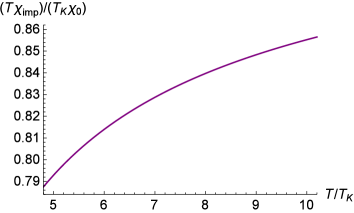
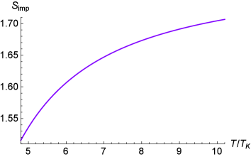
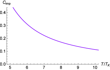
Figure 6: ($T\chi(T)$ [panel (a)], entropy (50) [panel (b)] and specific heat (51) [panel (c)] as functions of temperature $T$ in the weak coupling regime ${T}\gg{T_{K}}$.

The quantity $T\chi(T)$ are shown in Fig. 6. Within the realm of solid state physics, the mild logarithmic increase of $\chi(T)$ with decreasing temperature in the weak coupling regime of the Coqblin-Schrieffer model, has been discussed experimentally and theoretically a long time ago [see Ref.Hewson-book , page 258 Fig.(II)]. It would be of extreme interest to reveal it also within the realm of cold atom physics. For the isolated impurity, $T\chi(T)=T_{K}\chi_{0}$ is a constant (Curie law). The fact that $T\chi(T)$ decreases with temperature is a manifestation of the Kondo interaction of the impurity with the Fermi gas. In order to compare the standard SU(2) Kondo model with the SU($N$) Coqblin-Schrieffer model, we consider the quantity $X=(T\chi-T_{K}\chi_{0})/(T_{K}\chi_{0})$. For the SU(2) Kondo effect, $X=1/\ln(T/T_{K})$, whereas for the SU($N$) Coqblin-Schrieffer model $X=2/(N\ln(T/T_{K}))$, i.e., the additional factor $2/N$ appears.

Entropy and specific heat: Calculations of entropy and specific heat start from the free energy of the impurity $F_{\mathrm{imp}}=-T\ln(Z/Z_{0})$, where $Z$ is the partition function of the entire system and $Z_{0}$ is the partition function of the Fermi gas without the impurities,

$$Z={\mathrm{tr}}~{}e^{-\beta H},\ \ \ \ \ Z_{0}={\mathrm{tr}}~{}e^{-\beta H_{0}}$$ (49)

The impurity entropy is defined as,

$$S_{\mathrm{imp}}=-\frac{\partial F_{\mathrm{imp}}}{\partial T}.$$

Poor man’s scaling technique which is used in the weak coupling regime ${T}\gg{T}_{K}$ yield the following expression for the impurity contribution to the entropy Hewson-book :

$$S_{\mathrm{imp}} = \ln\big{(}N\big{)}-\frac{N^{2}-1}{N^{3}}~{}\frac{2\pi^{2}}{3\ln^{3}(T/T_{K})}.$$ (50)

The impurity specific heat $C_{\mathrm{imp}}=TdS_{\mathrm{imp}}/dT$ is,

$$C_{\mathrm{imp}} = \frac{N^{2}-1}{N^{3}}~{}\frac{2\pi^{2}}{\ln^{4}(T/T_{K})}.$$ (51)

The entropy (50) and the specific heat (51) as functions of temperature are displayed in Figs. 6 and 6. Kondo effect results in reducing of the entropy with decreasing temperature, whereas $C_{\mathrm{imp}}$ increases when temperature decreases. This is the manifestation of the Kondo effect. Note that for the standard SU(2) KE (which is the case $N=2$), both $S_{\mathrm{imp}}-\ln(2)$ and $C_{\mathrm{imp}}$ are proportional to the factor $3/8$, whereas for the SU($N$) Coqblin-Schrieffer model, the factor $(N^{2}-1)/N^{3}$ appears.

IV.2 Magnetization, specific heat and entropy in the strong coupling regime

For $T<T_{K}$, a non-perturbative method should be employed for calculating observables. This is worked out in Ref. Rajan-prl-83 , where the BA was applied for studying the Coqblin-Schrieffer model at low temperature. Here we apply the formalism derived therein for calculating the pertinent observables in thermal equilibrium. The general structure and behaviour of these quantities is expressed as universal functions of $T/T_{K}$. In particular, the magnetic susceptibility $\chi_{\mathrm{imp}}$, the ratio $S_{\mathrm{imp}}/T$ between the entropy and temperature and the ratio $C_{\mathrm{imp}}/T$ between the specific heat and the temperature are characterized by a finite temperature peak that becomes more dominant at larger $N$. This is the main difference between the standard SU(2) Kondo model and SU($N$) Coqblin-Schrieffer model: For the SU(2) KE, each one of these three quantities displays a zero temperature peak Rajan-prl-83 ; Hewson-book .

The contribution of the impurity to the free energy at a given magnetic field $B$ (and for $T<T_{K}$) reads Rajan-prl-83 ,

$$F_{\mathrm{imp}} = -T\sum_{\mu}\int{d\epsilon}~{}\rho_{\mathrm{sc}}\big{(}\epsilon-\mu\Delta_{B}\big{)}\ln\Big{(}1+e^{-\epsilon/T}\Big{)}+$$ (52)

$$+T\int{d\epsilon}~{}\rho_{\mathrm{sc}}\big{(}\epsilon\big{)}\ln\Big{(}1+e^{-\epsilon/T}\Big{)},$$

where

$$\Delta_{B}~{}=~{}g_{\mathrm{Yb}}\mu_{n}B,$$

the energy $\epsilon$ is measured with respect to the Fermi energy. Here $\rho_{\mathrm{sc}}(\epsilon)$ is the density of state (DOS) of fermions calculated in the strong coupling limit. At zero temperature, there is a peak in the DOS of width of order $T_{K}$ near the Fermi energy Hewson-book . This peak is calculated in the framework of slave boson mean field theory Hewson-book ; KA-prb14 ,

$$\rho_{\mathrm{sc}}(\epsilon) = \frac{1}{2}\sum_{\nu=\pm 1}\frac{\frac{\pi T_{K}}{N}}{\big{(}\epsilon-\nu\epsilon_{N}\big{)}^{2}+\left(\frac{\pi T_{K}}{N}\right)^{2}},$$ (53)

where $\epsilon_{N}=T_{K}\cos(\pi/N)$. Here we take into account that the electron excitations and hole excitations contribute equally to the free energy Rajan-prl-83 , and take $g(\epsilon)=g(-\epsilon)$.

Magnetic susceptibility: The zero field impurity magnetic susceptibility $\chi_{\mathrm{imp}}$, defined as

$$\chi_{\mathrm{imp}}~{}=~{}-\bigg{(}\frac{\partial^{2}F_{\mathrm{imp}}}{\partial B^{2}}\bigg{)}_{B\to 0},$$

is given by Rajan-prl-83 ,

$$\chi_{\mathrm{imp}} = \frac{\chi_{0}T_{K}}{12T}~{}N\big{(}N^{2}-1\big{)}\int\frac{\rho_{\mathrm{sc}}(\epsilon)d\epsilon}{\cosh^{2}\left(\frac{\epsilon}{2T}\right)},$$ (54)

where $\chi_{0}$ is given by Eq. (48).

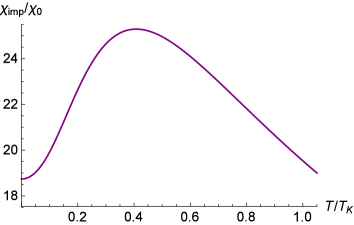
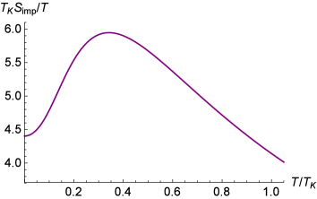
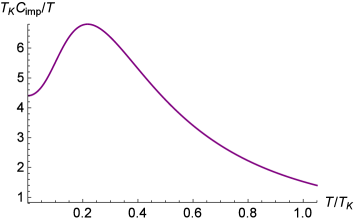
Figure 7: (Magnetic susceptibility (54) [panel (a)], $S_{\mathrm{imp}}/T$ [panel (b)] and $TC_{\mathrm{imp}}(T)$ [panel (c)] as functions of temperature in the strong coupling regime $T<T_{K}$

.

The magnetic susceptibility (54) is shown in Fig. 7.

Entropy: Differentiating the free energy (52) and letting the magnetic field $B\to 0$, we obtain an expression for the impurity entropy,

$$S_{\mathrm{imp}} = (N-1)\int{d\epsilon}~{}\rho_{\mathrm{sc}}\big{(}\epsilon\big{)}\ln\Big{(}1+e^{-\epsilon/T}\Big{)}+$$ (55)

$$+\frac{N-1}{T}\int{d\epsilon}~{}\epsilon\rho_{\mathrm{sc}}\big{(}\epsilon\big{)}f(\epsilon),$$

where $f(\epsilon)$ is the Fermi-Dirac distribution,

$$f(\epsilon)~{}=~{}\frac{1}{1+e^{\epsilon/T}}.$$

Specific heat: Differentiating the entropy, we get specific heat of the impurity Rajan-prl-83 ,

$$C_{\mathrm{imp}} = \big{(}N-1\big{)}\int\Big{(}\frac{\epsilon}{2T}\Big{)}^{2}~{}\frac{\rho_{\mathrm{sc}}(\epsilon)d\epsilon}{\cosh^{2}\left(\frac{\epsilon}{2T}\right)}.$$ (56)

The functions $S_{\mathrm{imp}}/T$ and $C_{\mathrm{imp}}/T$ are shown in Figs. 7 and 7.

V Conclusions

We have studied the feasibility of realizing the Coqblin-Schrieffer model in cold ¹⁷³Yb atoms. The peculiarities of this framework are as follows: 1) The same atoms are used as itinerant fermions and impurity atom, the only difference is that the former is in an excited state ³P₀ and the latter is in the atomic ground-state ¹S₀. 2) For both ground and excited states, the electronic total angular momentum is zero. 3) Therefore the ensuing exchange interaction is indirect and proceeds through virtual ionic states

$$[(6s^{2}),(6s6p)]\to[(6s^{2}6p)^{-},(6s)^{+}]\to[(6s6p),(6s^{2})].$$

The corresponding (positive) exchange energy between the localized and itinerant ytterbium atoms is calculated using reasonable models of atomic wave functions and experimental data for scattering lengths obtained in Ref. 6 . It is then incorporated within a Coqblin-Schrieffer Hamiltonian, and the Kondo temperature is estimated to be $T_{K}=~{}0.16\sim 0.31~{}T_{F}$ for $T_{F}=~{}50\sim 300$ nK. These conditions are favourable for the Kondo effect to be observed in cold fermionic ytterbium laboratories. Using renormalization group analysis, we calculated the magnetic susceptibility, entropy and specific heat of the impurity in the weak coupling regime, $T\gg{T}_{K}$. The temperature behaviour of these two quantities is in (qualitative) agreement with calculations carried out in heavy fermion systems, specifically for the $\Gamma_{8}$ quartet $S=\frac{3}{2}$ in a system of Ce impurity immersed in a LaB metal under cubic crystal field Schlottmann .

In the second step, we used the machinery of the Bethe Ansatz formalismBA for the calculation of the impurity contribution to the magnetic susceptibility, entropy and specific heat with the specific parameters pertaining to our Yb system (such as $J$, $T_{K}$, $N$, $g_{\mathrm{Yb}}$ and $\mu_{n}$). These results should consist of a reference starting point for relevant experiments.

Acknowledgements
Invaluable correspondence and discussion with Leonid Isaev are highly appreciated. The research of IK, TK and YA is partially supported by the Israel Science Foundation (ISF) under Grant 400/2012. G.B.J acknowledges financial support from the Hong Kong Research Grants Council (Project No.ECS26300014).

Appendix A Derivation of the Exchange Interaction

In this appendix we derive an expression for the exchange interaction between two atoms of ¹⁷³Yb. One of them (numbered 1) is the long-lived ³P₀ excited state with nuclear spin $\mu$, and the other one (numbered 2) is the ¹S₀ ground state with nuclear spin $\mu^{\prime}$. Each atom is considered as composed of an inert core (charge (+2) closed shell rigid ion) and two valence electrons, as illustrated in Fig. 2. The electron configuration of the excited state ³P₀ is $6s6p$, while that of the ground state ¹S₀ is $6s^{2}$. The positions of the ions are denoted as $\mathbf{R}_{\mathrm{e}}$ and $\mathbf{R}_{\mathrm{g}}$.

A.1 Indirect Exchange Interaction

In the present subsection we consider tunnelling of an electron from one atom to another which turns two neutral atoms into two ions or vice-versa, two ions into neutral atoms, as illustrated in Fig. 8. Explicitly, a 6$p$ electron tunnels from the atom in the excited state to the atom in the ground state. As a result, we have two ions with parallel electronic orbital moments [Fig. 8(b)]. Then one electron from the 6$s$ orbital tunnels from the negatively charged ion to the 6$s$ orbital of the positively charged ion. The net outcome is that the atoms “exchange their identity” specified by their electronic quantum states: one atom transforms from the ground state to the excited state, whereas the other atom transforms from the excited state to the ground state.

The Kohn-Sham scheme of density functional theory e-density-1996 ; e-density-ChemPhysLett-1997 ; e-density-JChemPhys-2002 ; e-density-Pollet-IntJQuantumChem-2003 ; e-density-Savin-IntJQuantumChem-2003 ; e-density-PhysRevA-2004 ; e-density-JChemPhys-2005 enables one to describe the long-range part of the potential created by an electron cloud as,

$$\Phi(R) = -\frac{2e}{R}~{}{\mathrm{erf}}\big{(}\mu R\big{)},$$ (57)

where $R$ is the distance from the nucleus and $1/\mu$ represents the distance beyond which the interaction reduces to the usual Coulomb long-range tail. The coefficient 2 in the numerator indicates 2 outer electrons of the Yb atom [namely, $6s^{2}$ or $6s6p$ electrons of the Yb(¹S₀) or Yb(³P₀) atom]. It is assumed that $\mu$ is the same for the $6s$ and $6p$ electrons. It is used below as a parameter for fitting the scattering lengths.

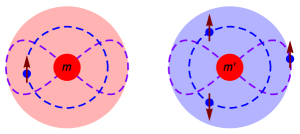
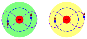
Figure 8: Illustration of exchange interaction between ytterbium atoms. Panel (a): Initial quantum state - the first atom (numbered 1) is in the meta-stable state (light yellow disk) and the second one (numbered 2) is in the ground state (light green disk); panel (b): virtual state - the first atom is positively ionized (light red disk), and the second one is negatively charged (light blue disk); panel (c): final state - the first atom is in the ground state and the other one is in the meta-stable state. For all the panels, arrows denote the electronic spin, $m$ or $m^{\prime}$ is nuclear spin of the first or second atom.

The Coulomb interaction between an electron and Yb(¹S₀) and Yb(³P₀) atoms separated by distance $R$ can be written as

$$V(\mathbf{r},\mathbf{R})=-\frac{2e^{2}}{\big{|}\mathbf{r}-\mathbf{R}/2\big{|}}~{}\Big{[}1-{\mathrm{erf}}\big{(}\mu|\mathbf{r}-\mathbf{R}/2|\big{)}\Big{]}$$

$$~{}~{}~{}~{}~{}~{}~{}~{}~{}~{}-\frac{2e^{2}}{\big{|}\mathbf{r}+\mathbf{R}/2\big{|}}~{}\Big{[}1-{\mathrm{erf}}\big{(}\mu|\mathbf{r}+\mathbf{R}/2|\big{)}\Big{]},$$ (58)

where $\mathbf{r}$ is the position of the electron, and $\pm\mathbf{R}/2$ are the positions of the atoms.

The tunnelling rate for an electron between the atoms can be calculated using the WKB approximation,

$$t_{\nu}(R) = \epsilon_{\nu}~{}e^{-2\gamma_{\nu}(R)},$$

$$\gamma_{\nu}(R) = \int\limits_{-z_{0}(\epsilon_{\nu})}^{z_{0}(\epsilon_{\nu})}\frac{\sqrt{2m_{e}}~{}dz}{\sqrt{\hbar^{2}\big{(}V(z,R)-\epsilon_{\nu}\big{)}}},$$ (59)

where $\nu=s,p$ for the $6s$ and $6p$ electrons, $m_{e}$ is the mass of electron, $V(z,R)$ is the potential energy (58) for $\mathbf{r}=(0,0,z)$ and $\mathbf{R}=(0,0,R)$, and $\pm z_{0}(\epsilon_{\nu})$ are classical turning points. The single-electron energies are $\epsilon_{s}=6.2542$ eV and $\epsilon_{p}=4.1107$ eV.

We calculate $t_{\nu}(R)$ numerically for different $R$ and found that it can be approximated by the simple function,

$$t_{\nu}(R) = t_{\nu}^{(0)}~{}e^{-2A_{\nu}^{(1)}(R-R_{0})},$$ (60)

where $R_{0}=4$ Å, $t_{\nu}^{(0)}=\epsilon_{\nu}e^{-2A_{\nu}^{(0)}}$, and $A_{\nu}^{(0)}$ and $A_{\nu}^{(1)}$ are given by

$$A_{s}^{(0)}=1.579,\ \ \ \ \ A_{s}^{(1)}=1.284~{}{\text{\AA}}^{-1},$$

$$A_{p}^{(0)}=0.943,\ \ \ \ \ A_{p}^{(1)}=1.044~{}{\text{\AA}}^{-1}.$$

Explicitly, $t_{s}^{(0)}=0.266$ eV and $t_{p}^{(0)}=0.248$ eV. Accordingly, the exchange interaction due to tunnelling of the $6s$ and $6p$ electrons is

$$g(R) = \frac{2t_{s}(R)t_{p}(R)}{\Delta\varepsilon},$$ (61)

where

$$\Delta\varepsilon = \varepsilon_{\mathrm{ion}}-\varepsilon_{\mathrm{ea}}+\epsilon_{1}-\epsilon_{2}~{}=~{}4.4107~{}{\mathrm{eV}},$$

where $\varepsilon_{\mathrm{ion}}=6.2542$ eV is the ionization energy Yb-spectrum-78 and $\varepsilon_{\mathrm{ea}}=-0.3$ eV is the electron affinity Electron-afinity-PhRep04 of ytterbium.

A.2 Semiclassical Wave Function in Atomic Scattering

Here we solve Schrödinger equation (20) in the framework of the semiclassical approximation Scatt-Length-WKB-PRA93 ; vdW-Yb-PRA-08 . The potential $W(R)$, Eq. (8), depends just on the distance $R$ from the impurity. Therefore, the orbital momentum $L$ and its projection $m$ on the axis $z$ are good quantum numbers. Because of the centrifugal barrier, atoms with nonzero $L$ cannot approach close one to another. Therefore we restrict ourselves by considering just the s-wave (i.e., the wave with $L=0$). Represent the wave function $\Psi_{r}(\mathbf{R})\equiv\Psi_{n}(\mathbf{R})$ as

$$\Psi_{n}(\mathbf{R}) = \frac{\psi_{n}(R)}{\sqrt{4\pi}~{}R}.$$ (62)

The radial wave function $\psi_{n}(R)$ satisfies the 1D Schrödinger equation,

$$\psi^{\prime\prime}_{n}(R)+\frac{M}{\hbar^{2}}~{}W(R)\psi_{n}(R)=0.$$ (63)

To solve this equation it is useful to employ different approximations in several corresponding intervals as defined below. To this end, we underline the following constraints on the parameters $R$: $r_{0}$, $b_{0}$ and $\lambda$ as follows:

• $r_{0}$ is determined from the equation $W(r_{0})=0$. The classical mechanics allows motion of the zero-energy particle in the interval $R>r_{0}$.

• $b_{0}$ is constrained by the inequality,

  $$\bigg{|}\frac{\sigma^{6}}{b_{0}^{6}}-\frac{C_{8}}{C_{6}b_{0}^{2}}\bigg{|}~{}\ll~{}1.$$

  For ${R}\geq{b}_{0}$, we can approximate $W(R)\approx-C_{6}/R^{6}$. Practically, we take $b_{0}\approx 10$ Å [see Fig. 3].

• $\lambda=(MC_{6}/\hbar^{2})^{1/4}=89.97$ Å. In principle, the WKB approximation can be used for for $R\ll\lambda$.

A brief list of approximations per intervals is as follows (see details below): For the interval $r_{0}<R\ll\lambda$, we can apply the WKB approximation to solve the Schrödinger equation (19). For the interval $b_{0}<R<\lambda$, we can approximate $W(R)$ by $-C_{6}/R^{6}$ and solve eq. (19). The interval $R<r_{0}$ corresponds to classically forbidden region where the wave function decays exponentially. In the following discussions, we find the wave function within each interval. The intervals $r_{0}<R\ll\lambda$ and $b_{0}<R<\lambda$ overlap one with another since there is a wide interval $b_{0}<R\ll\lambda$ where both the WKB approximation and the approximation $W(R)\approx-C_{6}/R^{6}$ are valid. Therefore, within this interval both the approaches should give the same solution. We use this condition as as a connection condition for the solutions within two overlapping intervals [see eqs. (69) and (74) below].

1. Interval $r_{0}<R\ll\lambda$: In order to solve equation (19), we apply the WKB approximation with quantum corrections vdW-Yb-PRA-08 . The wave function within this approximation is,

$$\psi_{n}^{(1)}(R) = \frac{A_{1n}}{\sqrt{K(R)}}~{}\sin\Big{(}\Phi_{r}(R)+\frac{\pi}{4}\Big{)},$$ (64)

where $A_{1n}$ is unknown constant,

$$\Phi_{r}(R) = \int\limits_{r_{0}}^{R}K(R^{\prime})dR^{\prime},$$ (65)

$$K(R) = \frac{1}{\hbar}~{}\sqrt{-MW(R)}.$$ (66)

Here the phase $\pi/4$ takes into account connection of $\psi_{n}^{(1)}(R)$ with exponentially decaying solution in the classically forbidden interval $R<r_{0}$ [see Ref. Scatt-Length-WKB-PRA93 ; vdW-Yb-PRA-08 ].

When $R>b_{0}$, we can write eq. (65) as,

$$\Phi_{r}(R)=\int\limits_{r_{0}}^{\infty}K(R^{\prime})~{}dR^{\prime}-\int\limits_{R}^{\infty}K(R^{\prime})~{}dR^{\prime}.$$ (67)

For any $R\geq{b}_{0}$, $K(R)$ can be approximated by $K_{0}(R)$ given by the equation,

$$K_{0}(R)~{}=~{}\frac{\sqrt{MC_{6}}}{\hbar R^{3}}~{}=~{}\frac{\lambda^{2}}{R^{3}}.$$

Then the second integral on the right hand side of eq. (67) can be performed analytically and gives,

$$\int\limits_{R}^{\infty}\frac{\lambda^{2}~{}dR^{\prime}}{\big{(}R^{\prime}\big{)}^{3}}~{}=~{}\frac{\lambda^{2}}{2R^{2}}.$$

Taking into account that the first term on the right hand side of eq. (67) is $\Phi_{w}$, eq. (30), we can write

$$\Phi_{r}(R)=\Phi_{w}-\frac{\lambda^{2}}{2R^{2}}.$$ (68)

Then $\psi_{n}^{(1)}(R)$ for $R>b_{0}$ takes the form,

$$\psi_{n}^{(1)}(R)=\frac{A_{1n}R^{3/2}}{\lambda}~{}\sin\Big{(}\Phi_{w}-\frac{\lambda^{2}}{2R^{2}}+\frac{\pi}{4}\Big{)}.$$ (69)

2. Interval $R>b_{0}$: Within this interval, we can approximate the potential energy by $W(R)\approx-C_{6}/R^{6}$ and write the Schrödinger equation (63) in the form,

$$\lambda^{2}~{}\frac{d^{2}\psi_{n}^{(2)}(R)}{dR^{2}}+\frac{\lambda^{6}}{R^{6}}~{}\psi_{n}^{(2)}(R) = 0,$$ (70)

where $\lambda$ is given by eq. (9).

General solution of eq. (70) is,

$$\psi_{n}^{(2)}(R) = A_{2n}~{}\tilde{\psi}_{2A}(R)+B_{2n}~{}\tilde{\psi}_{2B}(R),$$ (71)

where $\tilde{\psi}_{2A}(R)$ and $\tilde{\psi}_{2B}(R)$ are two linearly independent solutions of eq. (70),

$$\tilde{\psi}_{2A}(R) = \sqrt{\frac{2R}{\lambda}}~{}J_{1/4}\bigg{(}\frac{\lambda^{2}}{2R^{2}}\bigg{)},$$ (72a)

$$\tilde{\psi}_{2B}(R) = \sqrt{\frac{2R}{\lambda}}~{}J_{-1/4}\bigg{(}\frac{\lambda^{2}}{2R^{2}}\bigg{)},$$ (72b)

$A_{2n}$ and $B_{2n}$ are unknown constants.

When $R\gtrsim\lambda$, the asymptotic expressions for $\tilde{\psi}_{2A}(R)$ and $\tilde{\psi}_{2B}(R)$ are,

$$\tilde{\psi}_{2A}(R)=\frac{1}{\Gamma(5/4)}~{}\Bigg{\{}1-\frac{\lambda^{4}}{20R^{4}}+O\bigg{(}\frac{\lambda^{8}}{R^{8}}\bigg{)}\Bigg{\}},$$ (73a)

$$\tilde{\psi}_{2B}(R)=\frac{2R/\lambda}{\Gamma(3/4)}~{}\Bigg{\{}1-\frac{\lambda^{4}}{12R^{4}}+O\bigg{(}\frac{\lambda^{8}}{R^{8}}\bigg{)}\Bigg{\}}.$$ (73b)

For $R\ll\lambda$, the asymptotic expressions are,

$$\tilde{\psi}_{2A}(R)=\pi~{}\bigg{(}\frac{2R}{\pi\lambda}\bigg{)}^{3/2}\sin\bigg{(}\frac{\lambda^{2}}{2R^{2}}+\frac{\pi}{8}\bigg{)},$$ (74a)

$$\tilde{\psi}_{2B}(R)=\pi~{}\bigg{(}\frac{2R}{\pi\lambda}\bigg{)}^{3/2}\cos\bigg{(}\frac{\lambda^{2}}{2R^{2}}-\frac{\pi}{8}\bigg{)}.$$ (74b)

The functions $\tilde{\psi}_{2A}(R)$ and $\tilde{\psi}_{2B}(R)$, eq. (72), and their asymptotes (73) are shown in Fig. 4, solid and dashed lines. It is seen that for $R>\lambda$, the functions $\tilde{\psi}_{2A}(R)$ and $\tilde{\psi}_{2B}(R)$ are well approximated by their asymptotic expressions Scatt-Length-WKB-PRA93 .

There is a large interval $b_{0}<R\ll\lambda$, where we can approximate $W(R)$ by $-C_{6}/R^{6}$ and apply the WKB approximation. Therefore, we can apply the following connection conditions: For any $R$ within the interval $b_{0}<R\ll\lambda$, the equality $\psi_{n}^{(1)}(R)=\psi_{n}^{(2)}(R)$ is valid. This conditions gives,

$$A_{2n} = -A_{1n}~{}\frac{\sqrt{\pi\lambda}}{2}~{}\cos\Big{(}\Phi_{w}+\frac{\pi}{8}\Big{)},$$ (75a)

$$B_{2n} = A_{1n}~{}\frac{\sqrt{\pi\lambda}}{2}~{}\sin\Big{(}\Phi_{w}+\frac{3\pi}{8}\Big{)}.$$ (75b)

Taking into account eqs. (75) and (73), we can write the asymptote of the wave function $\psi_{n}^{(2)}(R)$, eq. (71), as $\psi_{n}^{(2)}(R)\propto{R-a_{w}}$, with the scattering length $a_{w}$ given by eq. (32) [see Refs. Scatt-Length-WKB-PRA93 ; vdW-Yb-PRA-08 ].

3. Interval $R\gtrsim\lambda$: Within this interval, the wave function is given by eq. (14). However, it is convenient to introduce a radial wave function $\psi_{3n}(R)$ similar to eq. (62),

$$\Psi_{\mathrm{g}}^{n00}(\mathbf{R})~{}=~{}\frac{\psi_{n}^{(3)}(R)}{\sqrt{4\pi}~{}R},$$

$$\psi_{n}^{(3)}(R)~{}=~{}\frac{2^{3/4}\sqrt{k_{n}}}{\sqrt{\pi}~{}b_{\mathrm{g}}}~{}\big{(}R-a_{w}\big{)},$$ (76)

where

$$k_{n}~{}=~{}\frac{2\sqrt{n}}{b_{\mathrm{g}}},$$ (77)

and $b_{\mathrm{g}}$ is the harmonic length (15). Here we take into account that $k_{n}\lambda\ll 1$ and $k_{n}a_{w}\ll 1$, and approximate $\psi_{3}(R)$ for $R\gtrsim\lambda$ by a linear function.

The wave function $\psi_{n}(R)$ and its derivative $\psi^{\prime}_{n}(R)$ are continues at $R=\lambda$. These conditions give

$$A_{1n} = \frac{2~{}\sqrt{k_{n}\lambda}}{\pi b_{\mathrm{g}}}~{}\Gamma\bigg{(}\frac{3}{4}\bigg{)}~{}\sqrt{1+\Big{(}\frac{a_{w}-\bar{a}}{\bar{a}}\Big{)}^{2}}.$$ (78)

A.3 Comparison of Our Calculations with the Results of Ref. Scazza-Yb-3P0-2015

In Ref. 6 , the authors report measurement of scattering lengths for two ytterbium atoms in the “singlet” and “triplet” two particle states [i.e., two particle states with symmetric and antisymmetric spatial wave function]. Explicitly, they are,

$$a_{S} = \big{(}1878\pm 37\big{)}~{}a_{B},$$ (79)

$$a_{T} = \big{(}219.7\pm 2.2\big{)}~{}a_{B}.$$ (80)

In order to compare our results with the measurements of Ref. 6 , we consider scattering of ytterbium atoms in the ground state with a localized impurity with taking into account van der Waals and exchange interaction. The van der Waals interaction between the ytterbium atoms is given by eq. (8) [see also Ref. vdW-Yb-PRA-08 ]. The exchange interaction between two atoms separated by distance $R$ is given by Eq. (61). Recall that positive $g(R)$ means that the corresponding exchange interaction is anti-ferromagnetic.

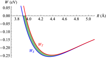
Figure 9: $W_{S}(R)$ and $W_{T}(R)$, eq. (83) [blue and red curves]. The green area indicates the exchange interaction (61).

The scattering length is given in Ref.vdW-Yb-PRA-08 in terms of a semiclassical (spin dependent) phase $\Phi$ by the following formula,

$$a_{\alpha} = \bar{a}~{}\Bigg{\{}1-\tan\bigg{(}\Phi_{\alpha}-\frac{\pi}{8}\bigg{)}\Bigg{\}},$$ (81)

where $\alpha=S$ or $T$ for the two-atomic state with spin wave function which is odd ($S$) or even ($T$) under permutation of the atoms, and $\bar{a}$ is given by eq. (33). The semiclassical phase $\Phi_{\alpha}$ is defined as vdW-Yb-PRA-08 [see eq. (23)],

$$\Phi_{\alpha} = \frac{\sqrt{M}}{\hbar}~{}\int\limits_{r_{\alpha}}^{\infty}\sqrt{-W_{\alpha}(R)}~{}dR,$$ (82)

where

$$W_{S}(R) = W(R)-g(R),$$

$$W_{T}(R) = W(R)+g(R).$$ (83)

$r_{S}$ or $r_{T}$ is a classical turning point for zero-energy particle found from the equation $W_{S}(r_{S})=0$ or $W_{T}(r_{T})=0$.

For a reference point, we also introduce the scattering length $a_{w}$ for pure van der Waals potential (without the exchange interaction). Of course, this quantity cannot be experimentally measured,

$$a_{w} = \bar{a}~{}\Bigg{\{}1-\tan\bigg{(}\Phi_{w}-\frac{\pi}{8}\bigg{)}\Bigg{\}},$$ (84)

where $\Phi_{w}(R)$ is given by eq. (30).

The potentials $W_{S}(R)$ and $W_{T}(R)$ are displayed in Fig. 9. It is seen that $W_{S}(R)$ lies below $W_{T}(R)$ which is evident due to the antiferromagnetic nature of the exchange interaction.

To proceed, we use $C_{8}$ and $\mu$ in Eqs. (8) and (61) as fitting parameters. For the best fit, we get

$$\Phi_{S}=297.318,\ \ \ \ \ \Phi_{T}=291.521,$$

$$\Phi_{w}=294.273,$$ (85)

and

$$a_{S}~{}=~{}1878~{}a_{B},\ \ a_{T}~{}=~{}219.7~{}a_{B},$$ (86)

$$a_{w}~{}=~{}650.6~{}{\text{\AA}}.$$ (87)

These values of $a_{S}$ and $a_{T}$ are close to the data given by Eqs. (79) and (80).

Figure 10: Scattering length as a function of the parameter $\Phi$ (blue curve). The red points are $a_{S}$ and $a_{T}$, the scattering lengths (86) for the “singlet” and “triplet” states, as well as $a_{w}$, the scattering length (87) for the pure van der Waals potential. The number of bound states increases by 1 as $\Phi$ increases and crossed a singularity. According to the sketch in the figure $N_{S}=N_{T}+1$.

A.4 Confinement-induced resonances

Following Ref. CIR-PhysRevA-2006 , we find “singlet” and “triplet” scattering lengths for itinerant Yb(³P₀) atoms scattered on trapped Yb(³P₀) impurity. When scattering length for two free atoms is $a$, scattering length for scattering of free atom on the impurity is

$$a_{\alpha} = 2a_{\alpha}^{(0)}\int\phi_{0}(r)\psi_{\mathrm{reg}}^{(\alpha)}(r)d^{3}\mathbf{r},$$ (88)

where $\alpha=S,T$ for the “singlet” and “triplet’ two-atomic state and $a_{\alpha}^{(0)}$ is the scattering lengths for two free atoms. $\phi_{0}(r)$ is the wave function of the ground state of a 3D harmonic oscillator describing the trapped atom, and $\psi_{\mathrm{reg}}^{k=0}(r)$ is defined as

$$\psi_{\mathrm{reg}}^{(\alpha)}(r) = \lim_{\rho\to 0}\frac{\partial}{\partial\rho}\Bigg{[}\rho~{}\psi_{\alpha}\bigg{(}\mathbf{r}+\frac{\bm{\rho}}{2},~{}\mathbf{r}-\frac{\bm{\rho}}{2}\bigg{)}\Bigg{]}.$$

Here the two-atomic wave function $\psi(\mathbf{r}_{\mathrm{g}},\mathbf{r}_{\mathrm{e}})$ is found from the equation,

$$\psi_{\alpha}(\mathbf{r}_{\mathrm{g}},\mathbf{r}_{\mathrm{e}}) = \phi_{0}(r_{B})+g_{\alpha}\int G_{E}^{(\alpha)}(\mathbf{r}_{\mathrm{g}},\mathbf{r}_{\mathrm{e}};\mathbf{r},\mathbf{r})$$ (89)

$$\times\psi_{\mathrm{reg}}^{(\alpha)}(r)~{}d^{3}\mathbf{r},$$

where

$$g_{\alpha}=\frac{4\pi\hbar^{2}a_{\alpha}^{(0)}}{M}.$$

Two-particle Green’s function is

$$G_{E}^{(\alpha)}(\mathbf{r}_{\mathrm{g}},\mathbf{r}_{\mathrm{e}};\mathbf{r},\mathbf{r})=-\frac{M}{2\pi\hbar^{2}}~{}\frac{1}{\big{|}\mathbf{r}_{\mathrm{g}}-\mathbf{r}\big{|}}$$

$$\times\sum_{\mathbf{n}}\phi_{\mathbf{n}}(\mathbf{r}_{\mathrm{e}})\phi_{\mathbf{n}}(\mathbf{r})~{}e^{-\kappa_{\mathbf{n}}|\mathbf{r}_{\mathrm{g}}-\mathbf{r}|},$$ (90)

where $\phi_{\mathbf{n}}(\mathbf{r})$ are wave functions of 3D harmonic oscillator in the state with harmonic numbers $\mathbf{n}=(n_{x},n_{y},n_{z})$,

$$\kappa_{\mathbf{n}}=\sqrt{\frac{2M\Omega_{\mathrm{e}}}{\hbar}~{}\big{(}n_{x}+n_{y}+n_{z}\big{)}},$$

and $\Omega_{\mathrm{e}}$ is the harmonic frequency.

Before solving numerically Eq. (89), we discuss, why the confinement can give rise to resonances? By the other words, why $a_{\mathrm{eff}}$ is singular? Eq. (89) can be formally written as

$$|\Psi_{\alpha}\rangle = |\Psi_{0}^{(\alpha)}\rangle+g_{\alpha}\hat{G}_{\epsilon}\hat{W}|\Psi_{\alpha}\rangle,$$ (91)

where the Green’s function is $\hat{G}_{\epsilon}=(\epsilon-H_{0}+i0)^{-1}$, and

$$\hat{W}\Psi\bigg{(}\mathbf{R}+\frac{\mathbf{r}}{2},\mathbf{R}-\frac{\mathbf{r}}{2}\bigg{)}=\delta(\mathbf{r})~{}\frac{\partial}{\partial r}\bigg{[}r~{}\Psi\bigg{(}\mathbf{R}+\frac{\mathbf{r}}{2},\mathbf{R}-\frac{\mathbf{r}}{2}\bigg{)}\bigg{]}.$$

Formal solution of Eq. (91) is

$$|\Psi_{\alpha}\rangle = \frac{1}{1-g_{\alpha}\hat{G}_{\epsilon}\hat{W}}~{}|\Psi_{0}^{(\alpha)}\rangle.$$ (92)

The operator $\hat{\mathcal{O}}=\hat{G}_{\epsilon}\hat{W}$ is a Hermitian operator, and it has real eigenvalues $\lambda_{i}$,

$$\hat{\mathcal{O}}|e_{i}\rangle=\lambda_{i}|e_{i}\rangle,$$

where $|e_{i}\rangle$ are eigenvactors of ${\mathcal{O}}$. Then the scattering length (88) can be written as CIR-PhysRevA-2006

$$a_{\alpha} = 2a_{\alpha}^{(0)}~{}\bigg{\langle}\tilde{\psi}_{0}^{(\alpha)}\bigg{|}\frac{1}{1-g_{\alpha}\hat{\mathcal{O}}}\bigg{|}\tilde{\psi}_{0}^{(\alpha)}\bigg{\rangle}$$ (93)

$$= \frac{M}{4\pi\hbar^{2}}\sum_{i}\frac{\big{|}\langle\tilde{\psi}_{0}^{(\alpha)}|e_{i}\rangle\big{|}^{2}}{g_{\alpha}^{-1}-\lambda_{i}},$$

where $\tilde{\psi}_{0}^{(\alpha)}(R)=R\Psi_{0}^{(\alpha)}(R,R)$. Singularity in $a_{\alpha}$ is expected when $g_{\alpha}^{-1}=\lambda_{i}$, or

$$a_{\alpha}^{(0)}=\frac{M}{4\pi\hbar^{2}\lambda_{i}}.$$

Since $\lambda_{i}$ is a function of $b_{\mathrm{e}}$ (the harmonic length of the trapped atom), the last equation allow us to calculate resonant values of $b_{\mathrm{e}}$.

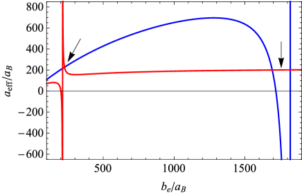
Figure 11: $a_{\mathrm{eff}}^{(S)}$ (blue curve) and $a_{\mathrm{eff}}^{(T)}$ (red curve) calculated numerically as functions of $b_{\mathrm{e}}$. The arrows show the intervals of $b_{\mathrm{e}}$ where $a_{\mathrm{eff}}^{(T)}>a_{\mathrm{eff}}^{(S)}$ and the exchange interaction turns from ferromagnetic to antiferromagnetic.

Solving Eq. (89) numerically and substituting $\psi_{\mathrm{reg}}^{(\alpha)}(r)$ into Eq. (88), we get $a_{\alpha}$ for the “singlet” ($\alpha=S$) and “triplet” ($\alpha=T$) two-atomic states. The results of the numerical calculations are shown in Fig. 11. It is seen that for most part of the interval $b_{\mathrm{e}}<1900a_{B}$, $a_{\mathrm{eff}}^{(S)}>a_{\mathrm{eff}}^{(T)}$, and the exchange interaction is ferromagnetic. However, there are two intervals, where $a_{\mathrm{eff}}^{(S)}<a_{\mathrm{eff}}^{(T)}$, and the exchange interaction is antiferromagnetic. The first one is close to a resonance for the “singlet” state,

$$1692a_{B}<b_{\mathrm{e}}<1819a_{B},$$

and the second one is close to a resonance for the “triplet” state,

$$212.8a_{B}<b_{\mathrm{e}}<226.7a_{B}.$$

Corresponding harmonic frequencies are

$$0.3026~{}\mu{\text{K}}<\frac{\hbar\Omega_{\mathrm{e}}}{k_{B}}<0.3497~{}\mu{\text{K}},$$ (94)

$$19.48~{}\mu{\text{K}}<\frac{\hbar\Omega_{\mathrm{e}}}{k_{B}}<22.11~{}\mu{\text{K}}.$$ (95)

Fig. 10 in Ref. CIR-PhysRevA-2006 show that there are more resonances corresponding to higher values of $\lambda_{i}$, but they are very narrow and do not considered here. In the following discussions, we demonstrate formation of CIRs for $a_{\alpha}^{(0)}>0$.

A.4.1 Estimation of resonant values of $\Omega_{\mathrm{e}}$

Here we follow Ref. CIR-PhysRevA-2006 and calculate resonant frequencies for $a_{\alpha}^{(0)}\ll b_{\mathrm{e}}$. In order to estimate resonant values of $\Omega_{\mathrm{e}}$, we write two-atomic Hamiltonian as

$$H = H_{R}+H_{r}+H_{\mathrm{int}},$$ (96)

where $\mathbf{R}=(\mathbf{r}_{\mathrm{g}}+\mathbf{r}_{\mathrm{e}})/2$ is the position of the center of mass and $\mathbf{r}=\mathbf{r}_{\mathrm{g}}-\mathbf{r}_{\mathrm{e}}$ is the relative coordinate.

$$H_{R} = -\frac{\hbar^{2}}{4M}~{}\frac{\partial^{2}}{\partial\mathbf{R}^{2}}+\frac{M\Omega_{\mathrm{e}}^{2}}{2}~{}R^{2},$$ (97)

$$H_{r} = -\frac{\hbar^{2}}{M}~{}\frac{\partial^{2}}{\partial\mathbf{r}^{2}}+g_{\alpha}~{}\delta(\mathbf{r})~{}\frac{\partial}{\partial r}\big{(}r\cdot\big{)},$$ (98)

$$H_{\mathrm{int}} = \frac{M\Omega_{\mathrm{e}}^{2}}{8}~{}r^{2}-\frac{M\Omega_{\mathrm{e}}^{2}}{2}~{}(\mathbf{R}\cdot\mathbf{r}).$$ (99)

$H_{r}$ describe relative motion of the atoms with van der Waals interaction (which is parametrized by the point-like interaction). Consider the situation when the atoms are trapped by the van der Waals interaction and form a molecule. Energy level of the weakest-bounded $s$ state is

$$\epsilon_{r}=-\frac{\hbar^{2}}{M\big{(}a_{\alpha}^{(0)}\big{)}^{2}}.$$

$H_{R}$ describes motion center of mass of the molecule which is trapped by the optical lattice potential and possesses harmonic oscillations. Harmonic frequency of the molecule is $\Omega_{\mathrm{e}}/\sqrt{2}$ and energies of the $s$ states are

$$\epsilon_{R}=\frac{\hbar\Omega_{\mathrm{e}}}{\sqrt{2}}~{}\bigg{(}2n+\frac{3}{2}\bigg{)},$$

where $n$ is an nonnegative integer. Corrections to the energies from $H_{\mathrm{int}}$ [which are of order $\hbar\Omega_{\mathrm{e}}\big{(}a_{\alpha}^{(0)}/b_{\mathrm{e}}\big{)}^{2}\ll\hbar\Omega_{\mathrm{e}}$] are small and can be neglected hereafter. Within this unperturbed approximation, $a_{\alpha}$ diverges each time the energy of the oscillating molecule is equal to the ground state energy of the pair of atoms, i.e. at the values of $\Omega_{\mathrm{e}}=\Omega_{n}^{(\alpha)}$ that satisfy

$$\bigg{(}2n+\frac{3}{2}\bigg{)}~{}\frac{\hbar\Omega_{n}^{(\alpha)}}{\sqrt{2}}-\frac{\hbar^{2}}{M\big{(}a_{\alpha}^{(0)}\big{)}^{2}}=\frac{3}{2}~{}\hbar\Omega_{n}^{(\alpha)}.$$ (100)

Solving Eq. (100) we find resonant harmonic frequencies,

$$\hbar\Omega_{n}^{(\alpha)} = \frac{\hbar^{2}}{M\big{(}a_{\alpha}^{(0)}\big{)}^{2}}~{}\frac{4}{\sqrt{2}(4n+3)-6)}.$$ (101)

Taking into account Eqs. (79) and (80), we get resonant frequencies for lowest $n$,

$$\begin{array}[]{|c|c|c|}\hline\cr n&\hbar\Omega_{n}^{(S)}/k_{B}(\mu{\text{K}})&\hbar\Omega_{n}^{(T)}/k_{B}(\mu{\text{K}})\\ \hline\cr 1&0.2913&21.29\\ \hline\cr 2&0.1189&8.686\\ \hline\cr 3&0.0747&5.456\\ \hline\cr 4&0.0544&3.978\\ \hline\cr\end{array}$$

The values for $n=1$ are close to values (94) and (95) calculated numerically.

References

- (1) I. Bloch, J. Dalibard, and W. Zwerger, Rev. Mod. Phys. 80, 885 (2008).
- (2) T. Bourdel, J. Cubizolles, L. Khaykovich, K.M.F. Magalhães, S.J.J.M.F. Kokkelmans, G.V. Shlyapnikov, and C. Salomon, Phys. Rev. Lett. 91, 020402 (2003).
- (3) S.J.J.M.F. Kokkelmans, G.V. Shlyapnikov, C. Salomon, Phys. Rev. A 69, 031602 (2004).
- (4) C. A. Regal and D. S. Jin, Adv. Atom. Mol. Opt. Phys. 54, 1 (2006).
- (5) Q.J. Chen, C.A. Regal, M. Greiner, D.S. Jin, and K. Levin, Phys. Rev. A 73, 041601 (2006).
- (6) Wenhui Li, G. B. Partridge, Y. A. Liao, and R. G. Hulet, Nuclear Physics A 790, 88c (2007).
- (7) Wolfgang Ketterle and Martin W. Zwierlein, in “Ultracold Fermi Gases”, Proceedings of the International School of Physics ”Enrico Fermi”, Course CLXIV, Varenna, 20 - 30 June 2006, edited by M. Inguscio, W. Ketterle, and C. Salomon (IOS Press, Amsterdam) 2008.
- (8) J. T. Stewart, J. P. Gaebler, and D. S. Jin, Nature 454, 744 (2008).
- (9) W. Li, G. B. Partridge, Y. A. Liao and R. G. Hulet, Int. J. of Mod. Phys. B 23, 3195 (2009).
- (10) S. Nascimbéne, N. Navon, K. J. Jiang, F. Chevy, and C. Salomon, Nature, 463, 1057 (2010).
- (11) N. Navon, S. Nascimbane, F. Chevy, and C. Salomon, Science 328, 729, (2010).
- (12) Marco Anderlini, Patricia J. Lee, Benjamin L. Brown, Jennifer Sebby-Strabley, William D. Phillips and J. V. Porto, Nature 448, 452 (2007).
- (13) S. Trotzky, P. Cheinet, S. Fölling, M. Feld, U. Schnorrberger, A. M. Rey, A. Polkovnikov, E. A. Demler, M. D. Lukin, and I. Bloch, Science 319, 295 (2008).
- (14) A. M. Kaufman, B. J. Lester, M. Foss-Feig, M. L. Wall, A. M. Rey, C. A. Regal, arXiv:1507.05586.
- (15) Jia Wang, Marko Gacesa, Robin Côté, Phys. Rev. Lett. 114, 243003 (2015); arXiv:1410.7853.
- (16) Russell A. Hart, Pedro M. Duarte, Tsung-Lin Yang, Xinxing Liu, Thereza Paiva, Ehsan Khatami, Richard T. Scalettar, Nandini Trivedi, David A. Huse, Randall G. Hulet, Nature 519, 211-214 (2015); arXiv:1407.5932.
- (17) C.A. Regal, C. Ticknor, J.L. Bohn and D.S. Jin, Nature 424, 47 (2003).
- (18) F. Ferlaino, S. Knoop, M. Berninger, M. Mark, H.-C. Naegerl and R. Grimm, Laser Phys. 20, 23 (2009); arXiv:0904.0935.
- (19) G. Barontini, C. Weber, F. Rabatti, J. Catani, G. Thalhammer, M. Inguscio and F. Minardi, Phys. Rev. Lett. 103, 043201 (2009).
- (20) S. Knoop, F. Ferlaino, M. Mark, M. Berninger, H. Schoebel, H.-C. Naegerl and R. Grimm, Nature Physics 5, 227 (2009).
- (21) M. Greiner, Ph.D. thesis, Ludwig Maximilian University of Munich, 2003.
- (22) Shintaro Taie, Yosuke Takasu, Seiji Sugawa, Rekishu Yamazaki, Takuya Tsujimoto, Ryo Murakami, and Yoshiro Takahashi, Phys. Rev. Lett. 105, 190401 (2010).
- (23) Yusuke Nishida, arXiv:1508.07098.
- (24) Masaya Nakagawa, Norio Kawakami, arXiv:1506.02947.
- (25) S. Lal, S. Gopalakrishnan and P. M. Goldbart, arXiv:0910.1579.
- (26) L.-M. Duan, E. Demler, and M. D. Lukin, Phys. Rev. Lett. 91, 090402 (2003).
- (27) D. C. McKay and B. DeMarco, Rep. Prog. Phys. 74, 054401 (2011).
- (28) Johannes Bauer, Christophe Salomon and Eugene Demler, Phys. Rev. Lett. 111, 215304 (2013).
- (29) I. Kuzmenko, T. Kuzmenko, Y. Avishai and K. A. Kikoin, Phys. Rev. B91, 165131 (2015); arXiv:1402.0187.
- (30) J.Kondo, Progr. Theor. Phys. 32, 37 (1964).
- (31) P. Coleman, Physics World 12, 29 (1995).
- (32) P. W. Anderson, Physics World 12, 37 (1995).
- (33) A. C. Hewson, The Kondo Problem to Heavy Fermions (Cambridge University Press, Cambridge, 1993).
- (34) V. T. Rajan, Phys. Rev. Lett. 51, 308 (1983).
- (35) P. Schlottmann, Zeitschrift für Physik B: Condensed Matter 51, 223 (1983).
- (36) Andrés Jerez, Natan Andrei, and Gergely Zaránd, Phys. Rev. B 58, 3814 (1998).
- (37) V. Zlatić, B. Horvatić, I. Milat, B. Coqblin, G. Czycholl, and C. Grenzebach, Phys. Rev. B 68, 104432 (2003); Physica B: Condensed Matter 312-313, 171 (2002); arXiv:cond-mat/0110179.
- (38) V.V. Bazhanov, S.L. Lukyanov, A.M. Tsvelik, Phys. Rev. B 68, 094427 (2003); arXiv:cond-mat/0305237.
- (39) Junya Otsuki, Hiroaki Kusunose, Philipp Werner and Yoshio Kuramoto, J. Phys. Soc. Jpn. 76, 114707 (2007); arXiv:0708.0718.
- (40) Igor Kuzmenko, Yshai Avishai, Phys. Rev. B89, 195110 (2014); arXiv:1310.6563.
- (41) H.-U. Desgranges, Physica B: Condensed Matter, 454, 135 (2014); arXiv:1309.3749.
- (42) Takeshi Fukuhara, Yosuke Takasu, Mitsutaka Kumakura, and Yoshiro Takahashi, Phys. Rev. Lett. 98, 030401 (2007).
- (43) Y.N.Martinez de Escobar, P.G. Mickelson, M. Yan, B.J. DeSalvo, S.B. Nagel, and T.C. Killian, Phys. Rev. Lett. 103, 200402 (2009).
- (44) S. Stellmer, R. Grimm, and F. Schreck, Physical Review A 84, 043611 (2011).
- (45) A.J.Daley Quantum Information Processing 10, 865 (2011).
- (46) Miguel A.Cazalilla and Ana Maria Rey, Reports on Progress in Physics 77, 124401 (2014).
- (47) Andrei Derevianko and Hidetoshi Katori, Reviews of Modern Physics 83, 331 (2011).
- (48) A. V. Gorshkov, M. Hermele, V. Gurarie, C. Xu, P. S. Julienne, J. Ye, P. Zoller, E. Demler, M. D. Lukin, and A. M. Rey, Nature Physics 6, 289 (2010).
- (49) Michael Foss-Feig, Michael Hermele and Ana Maria Rey, Physical Review A 81 051603 (2010).
- (50) Kaden R. A. Hazzard, Victor Gurarie, Michael Hermele, and Ana Maria Rey, Physical Review A 85 041604 (2012).
- (51) G. Cappellini, M. Mancini, G. Pagano, P. Lombardi, L. Livi, M. Siciliani de Cumis, P. Cancio, M. Pizzocaro, D. Calonico, F. Levi, C. Sias, J. Catani, M. Inguscio, and L. Fallani Phys. Rev. Lett. 113, 120402 (2014).
- (52) F. Scazza, C. Hofrichter, M. Fofer, P. C. De Groot, I. Bloch, and S. Folling, Nature Physics 10, 779 (2014); ibid: correction notice, (2015).
- (53) X. Zhang, M. Bishof, S. L. Bromley, C. V. Kraus, M. S. Safronova, P. Zoller, A. M. Rey, and J. Ye, Science 345, 1467 (2014).
- (54) S. K. Yip, B.-L. Huang and J.-S. Kao, Phys. Rev. A 89, 043610 (2014); arXiv:1312.6765. .
- (55) M. A. Cazalilla, A. F. Ho, and M. Ueda, New Journal of Physics, 11, 103033 (2009).
- (56) G. Pagano, M. Mancini, G. Cappellini, P. Lombardi, F. Schafer, H. Hu, X.-J. Liu, J. Catani, C. Sias, M. In- guscio, and L. Fallani, Nature Physics 10, 198 (2014).
- (57) R. Zhang, D. Zhang, Y. Cheng, W. Chen, P. Zhang, and H. Zhai, arXiv:1509.01350 (2015).
- (58) C. Pepin, P. Coleman, arXiv:cond-mat/0211284. ; P. Coleman, Lectures on the Physics of Highly Correlated Electron Systems VI, Editor F. Mancini, American Institute of Physics, New York (2002), p 79 - 160.
- (59) R. Zhang, Y. Cheng, H. Zhai, and P. Zhang, Phys. Rev. Lett. 115, 135301 (2015).
- (60) G. Pagano, M. Mancini, G. Cappellini, L. Livi, C. Sias, J. Catani, M. Inguscio, and L. Fallani, arXiv:1509.04256 (2015).
- (61) M. Hofer, L. Riegger, F. Scazza, C. Hofrichter, D. R. Fernandes, M. M. Parish, J. Levinsen, I. Bloch, and S. Folling, arXiv:1509.04257 (2015).
- (62) Yusuke Nishida, Phys. Rev. Lett. 111, 135301 (2013).
- (63) W. F. Meggers and J. L. Tech, J. Res. Natl. Bur. Stand. (U.S.) 83, 13 (1978).
- (64) W. F. Meggers and J. L. Tech, J. Res. Natl. Bur. Stand. (U.S.) 83, 13 (1978).
- (65) T. Andersen, “Atomic negative ions: Structure, dynamics and collisions”. Physics Reports 394, 157 (2004).
- (66) Masses, nuclear spins, and magnetic moments: I. Mills, T. Cvitas, K. Homann, N. Kallay, and K. Kuchitsu, in Quantities, Units and Symbols in Physical Chemistry, Blackwell Scientific Publications, Oxford, UK, 1988.
- (67) G. F. Gribakin and V. V. Flambaum, Phys. Rev. A 48, 546 (1993).
- (68) Masaaki Kitagawa, Katsunari Enomoto, Kentaro Kasa, Yoshiro Takahashi, Roman Ciuryło, Pascal Naidon, and Paul S. Julienne, Phys. Rev. A 77, 012719 (2008); arXiv:0708.0752.
- (69) S. G. Porsev, M. S. Safronova, A. Derevianko, and C. W. Clark, Phys. Rev. A 89, 012711 (2014).
- (70) P. Schlottmann, Solid State Commun. 57, 73 (1986).
- (71) A. M. Tsvelik and P. B. Wiegman, J. Phys. C 15, 1707 (1982); N. Andrei, K. Furuya and J. H. Lowenstein, Rev. Mod. Phys. 55 331 (1983).
- (72) L. Isaev and A. M. Rey, Phys. Rev. Lett. 115, 165302 (2015).
- (73) Cheng Chin, Rudolph Grimm, Paul Julienne and Eite Tiesinga, Rev. Mod. Phys. 82, 1225 (2010).
- (74) Caroline L. Blackley, Paul S. Julienne, and Jeremy M. Hutson, Phys. Rev. A 89, 042701 (2014).
- (75) A. Savin, in Recent Developments of Modern Density Functional Theory, edited by J. M. Seminario (Elsevier, Amsterdam, 1996), pp. 327Ð357.
- (76) T. Leininger, H. Stoll, H.-J.Werner, and A. Savin, Chem. Phys. Lett. 275, 151 (1997).
- (77) R. Pollet, A. Savin, T. Leininger, and H. Stoll, J. Chem. Phys. 4, 1250 (2002).
- (78) R. Pollet, F. Colonna, T. Leininger, H. Stoll, H.-J. Werner, and A. Savin, Int. J. Quantum. Chem. 91, 84 (2003).
- (79) A. Savin, F. Colonna, and R. Pollet, Int. J. Quantum. Chem. 93, 166 (2003).
- (80) J. Toulouse, F. Colonna, and A. Savin, Phys. Rev. A 70, 062505 (2004).
- (81) J. Toulouse, F. Colonna, and A. Savin, J. Chem. Phys. 122, 014110 (2005).
- (82) M. Höfer, L. Riegger, F. Scazza, C. Hofrichter, D. R. Fernandes, M. M. Parish, J. Levinsen, I. Bloch, and S. Fölling, Phys. Rev. Lett. 115, 265302 (2015).
- (83) T. Bergeman, M. G. Moore, M. Olshanii, Phys. Rev. Lett. 91, 163201 (2003); arXiv:cond-mat/0210556.
- (84) E. Haller, M. J. Mark, R. Hart, J. G. Danzl, L. Reichsöllner, V. Melezhik, P. Schmelcher, H.-C. Nägerl, Phys. Rev. Lett. 104, 153203 (2010); arXiv:1002.3795.
- (85) H. Moritz, T. Stöferle, K. Günter, M. Köhl, T. Esslinger, Phys. Rev. Lett. 94, 210401 (2005); arXiv:cond-mat/0503202.
- (86) P. Massignan and Y. Castin, Phys. Rev. A 74, 013616 (2006); arXiv:cond-mat/0604232.