Vertical Distribution Relations for Special Cycles on Unitary Shimura Varieties

Abstract.

We consider cycles on a 3-dimensional Shimura varieties attached to a unitary group, defined over extensions of a CM field $E$, which appear in the context of the conjectures of Gan, Gross, and Prasad [GGP09]. We establish a vertical distribution relation for these cycles over an anticyclotomic extension of $E$, complementing the horizontal distribution relation of [Jet15], and use this to define a family of norm-compatible cycles over these fields, thus obtaining a universal norm construction similar to the Heegner $\Lambda$-module constructed from Heegner points.

1. Introduction

Let $\mathcal{K}/\mathbb{Q}$ be an imaginary quadratic field with ring of integers $\mathcal{O}_{K}$ and let $\mathcal{N}$ be an ideal of $\mathcal{O}_{\mathcal{K}}$ of norm $N$. If $m$ is prime to $N$, the isogeny $\mathbb{C}/\mathcal{O}_{m}\to\mathbb{C}/(\mathcal{N}\cap\mathcal{O}_{m})^{-1}$ corresponds to a Heegner point $x_{m}$ in $X_{0}(N)(\mathcal{K}[m])$, where $\mathcal{K}[m]$ denotes the ring class field of conductor $m$ and $\mathcal{O}_{m}=\mathbb{Z}+m\mathcal{O}_{\mathcal{K}}$ is the corresponding order of $\mathcal{K}$.

Let $\mathcal{E}$ be an elliptic curve over $\mathbb{Q}$ of conductor $N$. For applications to anticyclotomic Iwasawa theory, one would like a module of universal norms in $\mathcal{E}(\mathcal{K}[p^{n}])$ as $n$ varies; that is, a collection of Heegner points $y_{p^{n}}\in E(\mathcal{K}[p^{n}])$ such that

(1) $$\operatorname{Tr}_{\mathcal{K}[p^{n+1}]/\mathcal{K}[p^{n}]}y_{p^{n+1}}=y_{p^{n}}.$$

The images $\widetilde{y}_{p^{n}}$ of the points $x_{p^{n}}$ constructed above under a fixed modular parametrization $X_{0}(N)\to\mathcal{E}$ do not satisfy this relation, but instead satisfy the “vertical distribution relation” (see [PR87, Lem.2]):

$$\operatorname{Tr}_{\mathcal{K}[p^{n+1}]/\mathcal{K}[p^{n}]}\widetilde{y}_{p^{n+1}}=a_{p}\widetilde{y}_{p^{n}}-\widetilde{y}_{p^{n-1}},\qquad n>1.$$

As explained in [Nek01, p.3], this relation, together with standard techniques from the theory of linear recurrences, allows one to modify the cycles $\widetilde{y}_{p^{n}}$ into a family satisfying (1).

This article establishes, under the assumption that $p$ is inert in the CM field, a vertical distribution relation for some higher-dimensional Shimura varieties, where the embedding of the non-split torus $\text{Res}_{\mathcal{K}/\mathbb{Q}}\mathbf{G}_{m}\to\operatorname{\mathbf{GL}}_{2}$ defining Heegner points is replaced by an embedding of unitary groups defining special one-dimensional cycles on a Shimura threefold. These cycles have their origin in the conjectures of Gan, Gross and Prasad [GGP09]; the intersection theory of variants of these cycles has been studied in the work of Howard [How12], and work on a Gross–Zagier formula for them has been initiated via the arithmetic fundamental lemma of Zhang [Zha12] and Rapoport, Terstiege and Zhang [RTZ13]. We work with the versions of these cycles defined in [Jet15], where a horizontal distribution relation is proven (again under the assumption that $p$ is inert).

1.1. Main theorem

Let $F$ be a totally real field and let $E/F$ be a totally imaginary quadratic extension, for which we pick once and for all an embedding into $\mathbb{C}$. Let $\tau$ be a finite prime of $F$, inert in $E$, and fix an embedding of $\overline{F}$ into $\overline{F}_{\tau}$; we will continue to write $\tau$ for the prime in any finite extension of $F$ by this choice. Let $W\subset V$ be an embedding of $E$-hermitian spaces with signatures $(1,1)$ (resp. $(2,1)$) at the distinguished real place of $F$ and $(2,0)$ (resp. $(3,0)$) at the other real places. One has algebraic groups $\mathbf{G}=\text{Res}_{E/F}(\mathbf{U}(V)\times\mathbf{U}(W))$ and $\mathbf{H}=\text{Res}_{E/F}\mathbf{U}(W)$, and an embedding $\mathbf{H}\hookrightarrow\mathbf{G}$, described in Section 2.1. In Section 2, a particular compact $K\subset\mathbf{G}(\mathbb{A}_{f})$ (for which $\tau$ is allowable in the sense of [Jet15, Defn.1.1], as recalled in Section 2.3), and Hermitian symmetric domain $X$ are chosen, which give rise to a Shimura variety $\operatorname{Sh}_{K}(G,X)$ and a family $\mathcal{Z}_{K}(\mathbf{G},\mathbf{H})$ of special one-cycles on this threefold. The cycles in $\mathcal{Z}_{K}(\mathbf{G},\mathbf{H})$ are defined over abelian extensions of $E$.

Attached to this data is the Hecke polynomial given by $\displaystyle H_{\tau}(z)=\sum_{i=0}^{6}C_{i}z^{i}\in\mathcal{H}_{\tau}[z]$, where $\mathcal{H}_{\tau}$ is a local Hecke algebra whose definition is recalled in Section 3.

Write $E[\tau^{n}]$ for the ring class field of $E$ of conductor $\tau^{n}$, that is, the abelian extension of $E$ whose norm subgroup is $E^{\times}\cdot\widehat{\mathcal{O}_{\tau^{n}}}^{\times}\subset\widehat{E}^{\times}$ where $\mathcal{O}_{\tau^{n}}=\mathcal{O}_{F}+\tau^{n}\mathcal{O}_{E}$ (here, $\tau^{n}$ denotes the $n$th power of the prime ideal of $\mathcal{O}_{F}$ corresponding to $\tau$). If $L$ is any extension of $E$, write $L[\tau^{n}]$ for the compositum $L\cdot E[\tau^{n}]$. Our main theorem holds under two assumptions:

Assumptions 1.1.

1. There exists a cycle $\xi_{1}\in\mathcal{Z}_{K}(\mathbf{G},\mathbf{H})$ defined over a finite extension $L$ of the Hilbert class field $E[1]$, which is abelian over $E$ and in which the chosen extension of $\tau$ to $E[1]$ splits completely.

2. The local invariants at $\tau$ (see Section 2.7 or [Jet15, Prop.3.4] for the definition) are given by $\operatorname{\mathbf{inv}}_{\tau}(\xi_{1})=(0,0)$.

Fixing such an $L$, the vertical distribution relation is then:

Theorem 1.2.

Suppose that $\tau$ is allowable for $(\mathbf{G},\mathbf{H},K)$ as defined in Paragraph 2.3. Under the assumptions listed in 1.1, there exists a family of cycles $\xi_{n}\in\mathcal{Z}_{K}(\mathbf{G},\mathbf{H})$ such that

• The field of definition of $\xi_{n}$ is $L[\tau^{n}]$ .

• For all sufficiently large $n$, one has

  $$\operatorname{Tr}_{L[\tau^{n+6}]/L[\tau^{n+5}]}\left(C_{6}\xi_{n+6}+\dots+C_{1}\xi_{n+1}+C_{0}\xi_{n}\right)=0.$$

Remark 1.

It would be useful to have arithmetic conditions to guarantee Assumption 1.1A in terms of a “Heegner hypothesis” on the pair $(E,K)$, particularly in the case that $L=E[1]$ is the Hilbert class field of $E$. This would require an extension of the results of [Jet15] to split and ramified primes. The case of general $L$ may be necessary for arithmetic applications (c.f. [AN10] for an instance where such a generalization is needed for $\operatorname{\mathbf{GL}}_{2}$) and the result is no harder to prove. Assumption (1.1)B holds for almost all allowable $\tau$, provided that Assumption(1.1)A holds.

As explained in Section 5, the above theorem can be used, together with a suitable choice of representation of the local group $\mathbf{U}(V)(F_{\tau})\times\mathbf{U}(W)(F_{\tau})$, to construct norm-compatible families $\{\widetilde{\xi}_{n}\}$.

There is a variant of this theorem using fewer terms, which may be more useful for computation – see Remark 4.

1.2. Strategy of proof

Theorem 1.2 would follow formally from the following “facts,” if they were true:

• There are operators $\mathcal{U}$ and $\mathcal{V}$ on $\mathcal{Z}_{K}(\mathbf{G},\mathbf{H})$ such that $\xi_{n}:=\mathcal{U}^{n}\xi_{0}$ is defined over $E[\tau^{n}]$ and, for sufficiently large $n$, $\mathcal{V}\xi_{n}=\xi_{n-1}$.

• This operator $\mathcal{V}$ is a formal root of the Hecke polynomial, in the sense that $H_{\tau}(\mathcal{V})$ induces the $0$ endomorphism of $\mathbb{Z}[\mathcal{Z}_{K}(\mathbf{G},\mathbf{H})]$.

Formalizing these “facts” is difficult on the level of the cycles themselves, but turns out to work on the level of the Bruhat–Tits building attached to ($\mathbf{G}$, $\tau$), which is a product of two trees. We recall the definitions of the cycles and buildings in Section 2, and then introduce the $\mathcal{V}$ operator in Section 3, showing that it is a root of the Hecke polynomial; we then show how to descend this to the level of cycles in Section 4. We conclude with Section 5, which explains how to build norm-compatible families.

2. Unitary Shimura Varieties

In this section we recall the constructions and notation of [Jet15, Section 2]. The reader is referred to loc. cit. for proofs and references for these facts.

2.1. Global fields and unitary groups

Write $D$ for the orthogonal complement of $W$ in $V$. Let $\mathbf{G}_{V}=\text{Res}_{F/\mathbb{Q}}\mathbf{U}(V)$ and $\mathbf{G}_{W}=\text{Res}_{F/\mathbb{Q}}\mathbf{U}(W)$; these are algebraic groups over $\mathbb{Q}$. The decomposition $V=W\perp D$ gives an embedding $\mathbf{G}_{W}\hookrightarrow\mathbf{G}_{V}$: if $R$ is a $\mathbb{Q}$-algebra, then $\mathbf{U}(W)(R)$ acts on $V\otimes R=(W\otimes R)\oplus(D\otimes R)$ by acting trivially on $D\otimes R$. Let $\mathbf{G}=\mathbf{G}_{V}\times\mathbf{G}_{W}$; there is a diagonal embedding

$$\Delta\colon\mathbf{G}_{W}\hookrightarrow\mathbf{G}.$$

Let $\mathbf{H}$ be the subgroup $\Delta(\mathbf{G}_{W})$ of $\mathbf{G}$.

Recall that we have fixed a prime $\tau$ of $F$ that is inert in $E$ and let $p$ be the rational prime below $\tau$. Let $q$ be the residue cardinality of $\tau$ (as a place of $F$), and choose a uniformizer $\varpi$ for $F_{\tau}$ (hence also for $E_{\tau}$).

Write $G_{V,\tau}=\mathbf{U}(V)(F_{\tau})$ and $G_{W,\tau}=\mathbf{U}(W)(F_{\tau})$. Let $G_{\tau}$ be the product $G_{V,\tau}\times G_{W,\tau}$ and write $H_{\tau}$ for the diagonally embedded copy of $G_{W,\tau}$ in $G_{\tau}$ (note that the symbol $H_{\tau}$ can denote either this group or the Hecke polynomial, depending on the context).

2.2. Hermitian symmetric domains

Let $X_{V}$ be the set of negative definite lines in $V\otimes\mathbb{R}$ (the tensor product taken with respect to the distinguished embedding), and similarly $X_{W}$ the set of negative definite lines in $W\otimes\mathbb{R}$.

Setting $X=X_{V}\times X_{W}$, the diagonal embedding $W\hookrightarrow V\oplus W$ induces an embedding of $X_{W}$ into $X$; write $Y$ for the image of $X_{W}$.

2.3. Compact-open subgroups of $\mathbf{G}(\mathbb{A}_{f})$

Fix a compact-open subgroup $K$ of $\mathbf{G}(\mathbb{A}_{f})$. We now make the assumption that $\tau$ is allowable for $(\mathbf{G},\mathbf{H},K)$ in the sense of [Jet15, Defn.1.1]; namely, writing $K_{\tau}$ for $K\cap\mathbf{G}_{\tau}\subset\mathbf{G}(\mathbb{A}_{f})$, we assume that

• The groups $\mathbf{U}(V)_{F_{\tau}}$ and $\mathbf{U}(W)_{F_{\tau}}$ are quasi-split.

• One has $K_{\tau}=K_{V,\tau}\times K_{W,\tau}$, where $K_{V,\tau}$ and $K_{W,\tau}$ are hyperspecial maximal compact subgroups of $G_{V,\tau}$ and $G_{W,\tau}$, respectively, and $K_{V,\tau}\cap G_{W,\tau}=K_{W,\tau}$ (the intersection taken under the given embedding).

• One has $K_{V,\tau}=K_{\tau}\times K_{V}^{(\tau)}$, where $K^{(\tau)}=K_{V}\cap\mathbf{U}(V)(\mathbb{A}_{F,f}^{(\tau)})$ (where $\mathbb{A}_{F,f}^{(\tau)}$ denotes the finite idèles outside of $\tau$)

This assumption implies that there is a Witt basis $\{e_{+},e_{0},e_{-}\}$ of the hermitian space $V_{\tau}:=V\otimes E_{\tau}$, i.e. a basis with respect to which the pairing is given by the matrix $\begin{pmatrix}0&0&1\\ 0&1&0\\ 1&0&0\end{pmatrix}$. Moreover, this basis has the properties that

• $W_{\tau}:=W\otimes E_{\tau}$ is spanned by $\{e_{+},e_{-}\}$.

• $K_{V,\tau}$ is the stabilizer in $G_{V,\tau}$ of the $\mathcal{O}_{E,\tau}$-lattice $\Lambda_{V}$ generated by $\{e_{+},e_{0},e_{-}\}$.

• $K_{W,\tau}$ is the stabilizer in $G_{W,\tau}$ of the $\mathcal{O}_{E,\tau}$-lattice $\Lambda_{W}$ generated by $\{e_{+},e_{-}\}$.

Note that the lattices $\Lambda_{V}$ and $\Lambda_{W}$ are self-dual.

2.4. Complex Shimura varieties and special cycles

The data $(\mathbf{G},X)$ and $(\mathbf{H},Y)$ satisfy Deligne’s axioms for Shimura data; one computes (see e.g. [Jet15, §2.2.6]) that the reflex field is $E$ in both cases, and thus there are varieties defined over $E$ whose complex points are given by

$$\operatorname{Sh}_{K_{V}}(\mathbf{G}_{V},X_{V})(\mathbb{C})=\mathbf{G}_{V}(\mathbb{Q})\backslash(\mathbf{G}_{V}(\mathbb{A}_{f})\times X_{V})/K_{V},$$

$$\operatorname{Sh}_{\Delta(K_{W})}(\mathbf{H},Y)(\mathbb{C})=\mathbf{H}(\mathbb{Q})\backslash(\mathbf{H}(\mathbb{A}_{f})\times Y)/\Delta(K_{W}).$$

One also has $\operatorname{Sh}_{K}(\mathbf{G},X)=\operatorname{Sh}_{K_{V}}(\mathbf{G}_{V},X_{V})\times\operatorname{Sh}_{K_{W}}(\mathbf{G}_{W},X_{W})$, with complex points given by

$$\operatorname{Sh}_{K}(\mathbf{G},X)(\mathbb{C})=\mathbf{G}(\mathbb{Q})\backslash(\mathbf{G}(\mathbb{A}_{f})\times X)/K.$$

For any $g\in\mathbf{G}(\mathbb{A}_{f})$, there is a “special cycle” $\mathcal{Z}_{K}(g)$, which is the image of $gK\times Y$ in $\operatorname{Sh}_{K}(\mathbf{G},X)(\mathbb{C})$; it is a subvariety of $\operatorname{Sh}_{K}(\mathbf{G},X)_{\mathbb{C}}$. Let $\mathcal{Z}_{K}(\mathbf{G},\mathbf{H})$ denote the set of all cycles obtained in this way. It is shown in [Jet15, §2.3] that the association $g\mapsto\mathcal{Z}_{K}(g)$ induces a bijection

$$\mathcal{Z}_{K}(\mathbf{G},\mathbf{H})\simeq\text{N}_{\mathbf{G}(\mathbb{Q})}(\mathbf{H}(\mathbb{Q}))\backslash\mathbf{G}(\mathbb{A}_{f})/K,$$

where the normalizer is explicitly given by

$$\text{N}_{\mathbf{G}(\mathbb{Q})}(\mathbf{H}(\mathbb{Q}))=\Delta(\mathbf{H}(\mathbb{Q}))\left(\underbrace{1\times\mathbf{U}(W^{\perp})(\mathbb{Q})}_{\subset{\mathbf{G}_{V}(\mathbb{Q})}}\times\underbrace{\mathbf{Z}_{\mathbf{H}}(\mathbb{Q})}_{\subset{\mathbf{G}_{W}}(\mathbb{Q})}\right)\subset\mathbf{G}(\mathbb{Q}).$$

2.5. Galois action on cycles

It is shown in [Jet15, §2.3], using Shimura reciprocity, that the cycles $\mathcal{Z}_{K}(g)$ are defined over abelian extensions of $E$. Explicitly, given $\sigma\in\text{Gal}(E^{\text{ab}}/E)$, let $s_{\sigma}\in\mathbb{A}_{E}^{\times}$ be any element such that $\text{Art}_{E}(s_{\sigma})=\sigma$ where

$$\operatorname{Art}_{E}\colon E^{\times}\backslash\mathbb{A}_{E}^{\times}\rightarrow\text{Gal}(E^{\text{ab}}/E)$$

is the Artin map. Let $\mathbf{T}^{1}=\mathbf{U}^{1}_{\mathbb{Q}}$ and let $\nu\colon\mathbf{H}\to\mathbf{T}^{1}$ be the determinant map. Consider the homomorphism $r=(r_{f},r_{\infty})\colon\mathbb{A}_{E}^{\times}\to\mathbf{T}^{1}(\mathbb{A})$ defined by $r(s)={\overline{s}}/{s}$. Then there exists $h_{\sigma}\in\mathbf{H}(\mathbb{A}_{f})$ such that $\nu(h_{\sigma})=r_{f}(s)$, and for any such choice, one has

(2) $$\sigma(\mathcal{Z}_{K}(g))=\mathcal{Z}_{K}(h_{\sigma}g).$$

This description implies that the Galois orbits of cycles receive a surjection

$$\mathbf{H}(\mathbb{A}_{f})\backslash\mathbf{G}(\mathbb{A}_{f})/K\twoheadrightarrow\text{Gal}(E^{\text{ab}}/E)\backslash\mathcal{Z}_{K}(\mathbf{G},\mathbf{H}).$$

The allowability hypothesis (Section 2.3) implies that domain of this map is of the form

$$H_{\tau}\backslash G_{\tau}/K_{\tau}\times\mathbf{H}(\mathbb{A}_{f}^{(\tau)})\backslash\mathbf{G}(\mathbb{A}_{f}^{(\tau)})/K^{(\tau)}.$$

2.6. Buildings for unitary groups

The local factor $H_{\tau}\backslash G_{\tau}/K_{\tau}$ appearing in the domain of the map above can be described in terms of the Bruhat–Tits building for $G_{\tau}$. This building is a product of two buildings; one for $G_{V,\tau}$ and the other for $G_{W,\tau}$. Each of these buildings is, in turn, isomorphic to a bicolored graph which we now describe. The reader is referred to [Kos13, §4.1] for proofs of the facts below and more details on the buildings, and to [Jet15, Figure 1] for a picture.

A “hyperspecial lattice” is a lattice $L$ of $V_{\tau}$ which is self-dual, and a “special lattice” $L$ is a lattice which is almost self-dual, which means that one has strict containments $\varpi L^{\vee}\subsetneq L\subsetneq L^{\vee}$. The (underlying bicolored graph of the) Bruhat–Tits building for $G_{V,\tau}$, which we denote by $\mathcal{B}(V_{\tau})$, consists of a black vertex for each hyperspecial lattice, and a white vertex for each special lattice. Two vertices are connected by an edge if and only if the corresponding lattices have index $q$ in one another. One calculates that each black vertex has $q^{3}+1$ white neighbors and each white vertex has $q+1$ black neighbors. A choice $\{f_{+},f_{0},f_{-}\}$ of Witt basis for $V_{\tau}$ determines an apartment in this building whose hyperspecial vertices are the self-dual lattices $\langle\pi^{m}f_{+},f_{0},\pi^{-m}f_{-}\rangle$ for $m\in\mathbb{Z}$; a “half-apartment” is the subset of an apartment where $m\geq n$ for some fixed $n$.

One defines $\mathcal{B}(W_{\tau})$ similarly; in this case, each black vertex has $q+1$ white neighbors, and each white vertex has $q+1$ black neighbors.

The building $\mathcal{B}(G_{\tau})$ is then the product of these graphs. The group $G_{\tau}$ acts on $\mathcal{B}(G_{\tau})$, preserving incidence relations and geodesics. As this action is transitive on the set of pairs of hyperspecial lattices, the quotient $G_{\tau}/K_{\tau}$ is identified with the set of (pairs of) black vertices in $\mathcal{B}(G_{\tau})$. The black vertices of $\mathcal{B}(V_{\tau})$, resp. $\mathcal{B}(W_{\tau})$, resp. the pairs of black vertices in $\mathcal{B}(G_{\tau})$ will be described in the sequel as $\operatorname{\mathbf{Hyp}}_{V,\tau}$, resp. $\operatorname{\mathbf{Hyp}}_{W,\tau}$, resp. $\operatorname{\mathbf{Hyp}}_{\tau}$. The sets $\operatorname{\mathbf{Hyp}}_{V,\tau}$ and $\operatorname{\mathbf{Hyp}}_{W,\tau}$ are endowed with distance functions, normalized so that the distance between two neighboring black points (i.e. two black points that share a white neighbor in the bicolored graph) is $1$.

Note that the choice of lattices in Section 2.3 distinguishes a particular black vertex in each graph; we will informally refer to this vertex as the “origin,” and to their product as the “origin” in the product building.

2.7. Galois action via Bruhat–Tits buildings

One can use the building to compute the orbits of the Galois action on the cycles. Given a point $x=(L_{V_{\tau}},L_{W_{\tau}})\in\mathbf{Hyp}_{\tau}$, write

$$\operatorname{\mathbf{inv}}_{\tau}(x):=\left(\text{dist}(L_{V_{\tau}},\operatorname{pr}_{W_{\tau}}(L_{V_{\tau}})),\text{dist}(L_{W_{\tau}},\operatorname{pr}_{W_{\tau}}(L_{V_{\tau}}))\right),$$

where $\operatorname{pr}_{W_{\tau}}$ is the projection as in [Jet15, §3]. The following result classifies the $H_{\tau}$-orbits in $\mathbf{Hyp}_{\tau}$ [Jet15, Prop.3.4]

Proposition 2.1.

Two hyperspecial points $x,y\in\mathbf{Hyp}_{\tau}$ lie in the same $H_{\tau}$-orbit if and only if $\operatorname{\mathbf{inv}}_{\tau}(x)=\operatorname{\mathbf{inv}}_{\tau}(y)$.

Write $\mathbb{U}^{1}(n):=\nu_{\tau}(\mathcal{O}_{n}^{\times})$, where $\nu_{\tau}\colon E_{\tau}^{\times}\to\mathbb{U}^{1}(L_{\tau})$ is given by $\nu_{\tau}(s)=\overline{s}/s$, and $\mathcal{O}_{n}=\mathcal{O}_{E,\tau}+\varpi^{n}\mathcal{O}_{F,\tau}$. The Shimura reciprocity law implies that

$$\det{\text{Stab}_{H_{\tau}}(L_{V_{\tau}},L_{W_{\tau}})}=\mathbb{U}^{1}(c_{\tau}([L_{V_{\tau}},L_{W_{\tau}}])),$$

where $c_{\tau}$ denotes the local conductor given by [Jet15, Thm.1.1], i.e.

$$c_{\tau}([L_{V_{\tau}},L_{W_{\tau}}]):=q^{\min\{\text{dist}(L_{V_{\tau}},\operatorname{pr}_{W_{\tau}}(L_{V_{\tau}})),2\text{dist}(L_{W_{\tau}},\ \operatorname{pr}_{W_{\tau}}(L_{V_{\tau}}))\}}.$$

3. Hecke operators and partial Hecke operators

3.1. The Hecke polynomial

The local Hecke algebra $\mathcal{H}_{\tau}=\mathcal{H}(G_{\tau},K_{\tau})$ is the set of $K_{\tau}$-bi-invariant continuous compactly-supported $\mathbb{Z}$-valued functions on $G_{\tau}$. There are natural actions of $\mathcal{H}_{\tau}$ on $\mathcal{B}(G_{\tau})$ and on the space $\mathcal{Z}_{K}(\mathbf{G},\mathbf{H})$, compatible with the map defined at the end of Section 2.5. Explicitly, given an element $g\in G_{\tau}$, let $\mathbf{1}_{K_{\tau}gK_{\tau}}$ be the characteristic function of the double coset $K_{\tau}gK_{\tau}$ (such functions generate $\mathcal{H}_{\tau}$). This acts on both $\operatorname{\mathbf{Hyp}}_{\tau}$ and $\mathcal{Z}_{K}(\mathbf{G},\mathbf{H})$ as follows: if $K_{\tau}gK_{\tau}=\sqcup g_{i}K_{\tau}$, then for $h\in G_{\tau}$, the corresponding endomorphism is $[h]\mapsto\sum[hg_{i}]$, where $[h]$ denotes the class of $h$ in either $G_{\tau}/K_{\tau}$ or the cycle $\mathcal{Z}_{K}(\ldots,1,1,h,1,1,\ldots)\in\mathcal{Z}_{K}(\mathbf{G},\mathbf{H})$, respectively.

Given a co-character $\mu$ of $\widehat{\mathbf{G}}$, there is a polynomial $H_{\tau}(z)$ with coefficients in $\mathcal{H}_{\tau}$, called the Hecke polynomial (this polynomial is originally defined by Langlands; we use the version of Blasius-Rogawski found in [BR94, §6]). An explicit formula for the Hecke polynomial is given in our setting by [Jet15, Thm.4.1].

To state that formula, let $\delta_{V}=\text{diag}(\varpi,1,\varpi^{-1})\in G_{V,\tau}$ and $\delta_{W}=\text{diag}(\varpi,\varpi^{-1})\in G_{W,\tau}$, where matrices are written with respect to the bases chosen in Section 2.3. Consider the Hecke operators $t_{1,0}=\mathbf{1}_{K_{\tau}(\delta_{V},1)K_{\tau}}$ and $t_{0,1}=\mathbf{1}_{K_{\tau}(1,\delta_{W})K_{\tau}}$. These act as adjacency operators on $\mathbb{Z}[\operatorname{\mathbf{Hyp}}_{\tau}]$; the former is the identity on $\operatorname{\mathbf{Hyp}}_{W,\tau}$ and sends a point in $\operatorname{\mathbf{Hyp}}_{V,\tau}$ to the formal sum of its neighbors, and similarly for the latter. Then one has:

Theorem 3.1.

The Hecke polynomial $H_{\tau}(z)\in\mathcal{H}_{\tau}[z]$ at the place $\tau$ for the Shimura datum $(\mathbf{G},X)$ is given by

$$H_{\tau}(z)=H^{(2)}(z)H^{(4)}(z)$$

where

$$H^{(2)}(z)=z^{2}-q^{2}(t_{0,1}-(q-1))z+q^{6}$$

and

$$H^{(4)}(z) =z^{4}$$

$$+(-t_{1,0}t_{0,1}+(q-1)(t_{1,0}+t_{0,1})-(q-1)^{2})z^{3}$$

$$+q^{2}(t_{1,0}^{2}+q^{2}t_{0,1}^{2}-2(q-1)t_{1,0}-2q^{2}(q-1)t_{0,1}-q^{4}-2q^{3}+2q^{2}-2q+1)z^{2}$$

$$+q^{6}(-t_{1,0}t_{0,1}+(q-1)(t_{1,0}+t_{0,1})-(q-1)^{2})z$$

$$+q^{12}.$$

Define the elements $C_{i}\in\mathcal{H}_{\tau}$ by $H_{\tau}(z)=C_{0}z^{6}+C_{1}z^{5}+\dots+C_{6}$ for $i=0,1,\dots,6$.

3.2. Partial Hecke operators

We will make use of a formal factorization of the Hecke polynomial in a ring extension of $\mathcal{H}_{\tau}$. Let $R_{V}=\operatorname{End}(\mathbb{Z}_{(p)}[\operatorname{\mathbf{Hyp}}_{V,\tau}])$, $R_{W}=\operatorname{End}(\mathbb{Z}_{(p)}[\operatorname{\mathbf{Hyp}}_{W,\tau}]$, and $R=R_{V}\otimes R_{W}=\operatorname{End}(\mathbb{Z}_{(p)}[\operatorname{\mathbf{Hyp}}_{\tau}])$, where $\mathbb{Z}_{(p)}$ denotes the localization of $\mathbb{Z}$ at $p$. The previously-defined actions on the buildings give an algebra map $\mathcal{H}_{\tau}\to R$ and a group map $H_{\tau}\to R^{\times}$.

We define predecessor and successor operators in $R_{V}$ and $R_{W}$. To keep the analogy with the case of $\operatorname{\mathbf{GL}}_{2}$, we use the notation $\mathcal{U}$ for operators which raise the distance of a point from the origin, and $\mathcal{V}$ for operators which lower it.

Thus, given a self-dual lattice $L\neq\Lambda_{V}$ in $\mathcal{B}(G_{V,\tau})$, set:

• $\mathcal{U}_{V}L=\sum L^{\prime}$, where the sum is taken over the self-dual lattices $L^{\prime}$ of $V_{\tau}$ such that $\mathrm{dist}(L,L^{\prime})=1\text{ and }\mathrm{dist}(L^{\prime},\Lambda_{V})>\operatorname{dist}(L,\Lambda_{V})$.

• $\mathcal{V}_{V}L$ is the unique self-dual lattice $L^{\prime}$ of $V_{\tau}$ such that $\mathrm{dist}(L,L^{\prime})=1$ and $\mathrm{dist}(L^{\prime},\Lambda_{V})<\operatorname{dist}(L,\Lambda_{V})$.

• $\mathcal{S}_{V}L=L+\sum L^{\prime}$, where the sum is taken over the self-dual lattices $L^{\prime}$ of $V_{\tau}$ such that $\mathrm{dist}(L,L^{\prime})=1\text{ and }\mathrm{dist}(L^{\prime},\Lambda_{V})=\operatorname{dist}(L,\Lambda_{V})$.

To complete the definition of these three operators, writing $x_{V}$ for the point corresponding to $\Lambda_{V}$, and $S_{1}$ for the formal sum of points of distance $1$ from the origin, and set:

• $\displaystyle\mathcal{U}_{V}x_{V}=\frac{q}{q+1}S_{1}$

• $\displaystyle\mathcal{V}_{V}x_{V}=(1-q^{3})x_{V}+\frac{1}{q+1}S_{1}$

• $\displaystyle\mathcal{S}_{V}x_{V}=q^{3}x_{V}$

(This definition is motivated by Lemma 3.2 below.)

Define the operators $\mathcal{U}_{W}$, $\mathcal{V}_{W}$, and $\mathcal{S}_{W}$ analogously, replacing both instances of $q^{3}$ with $q$ in the above definition. We will abuse notation and consider these as elements of $R$, e.g. writing $\mathcal{U}_{W}$ rather than $\mathcal{U}_{W}\otimes 1.$ These operators do not commute with each other. They are depicted in Figure 1.

Remark 2.

In the definition of $R$, the localization of the ring of coefficients at $p$ is necessary only to define the operators above at the origin. The cycles occurring in the main theorem, a priori in $\mathbb{Z}_{(p)}[\mathcal{Z}_{K}(\mathbf{G},\mathbf{H})]$, are in fact in $\mathbb{Z}[\mathcal{Z}_{K}(\mathbf{G},\mathbf{H})]$.

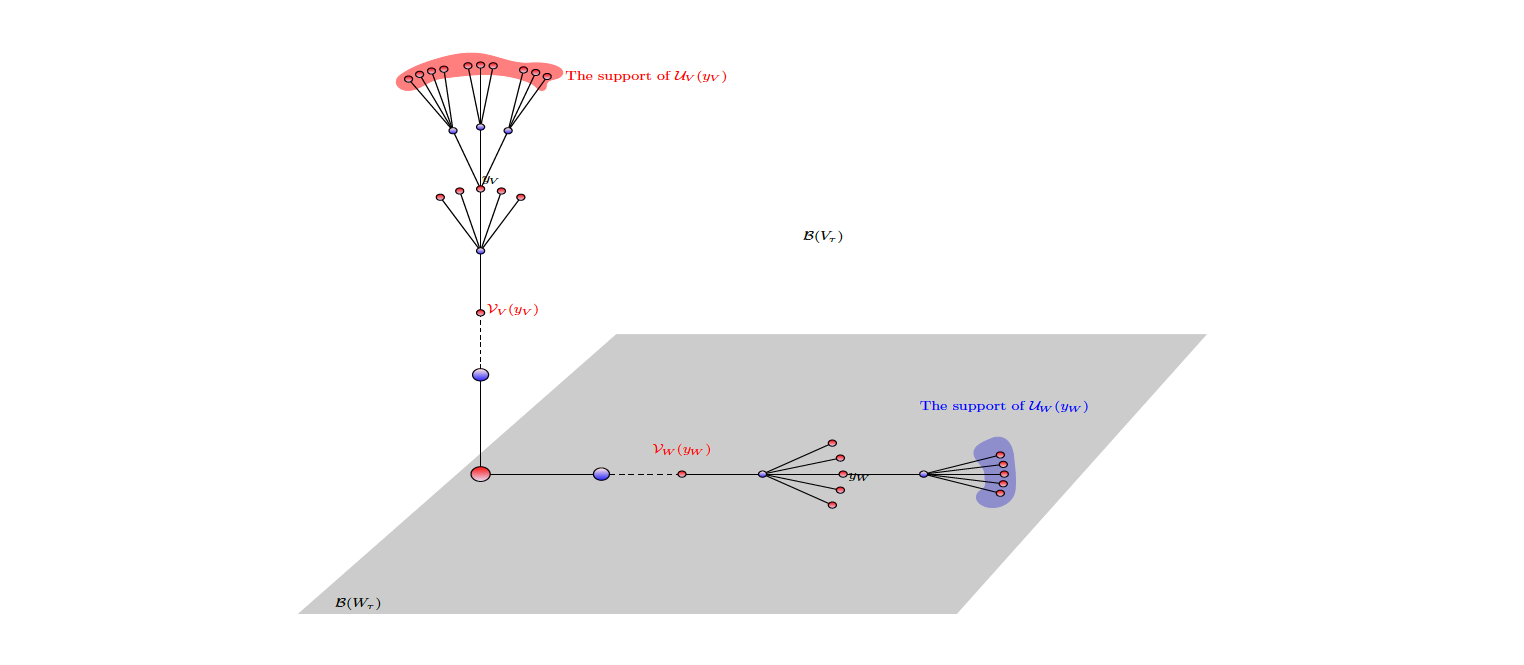
Figure 1. Examples of elements of $R$.

We gather the composition relations between the various operators in the following lemma; in each case, the proof (away from the origin) is a simple counting argument.

Lemma 3.2.

In $R$, one has

• $\mathcal{V}_{V}\mathcal{U}_{V}=q^{4}$ and $\mathcal{V}_{W}\mathcal{U}_{W}=q^{2}$

• $\mathcal{V}_{V}+\mathcal{U}_{V}+\mathcal{S}_{V}=t_{1,0}+1$ and $\mathcal{V}_{W}+\mathcal{U}_{W}+\mathcal{S}_{W}=t_{0,1}+1$.

• $\mathcal{V}_{V}\mathcal{S}_{V}=q^{3}\mathcal{V}_{V}$ and $\mathcal{V}_{W}\mathcal{S}_{W}=q\mathcal{V}_{W}$.

• $\mathcal{S}_{V}\mathcal{U}_{V}=q^{3}\mathcal{U}_{V}$ and $\mathcal{S}_{W}\mathcal{U}_{W}=q\mathcal{U}_{W}$.

• $(\mathcal{S}_{V})^{2}-q^{3}(\mathcal{S}_{V})=0$ and $(\mathcal{S}_{W})^{2}-q(\mathcal{S}_{W})=0$.

We say that an element of $\mathbb{Z}_{(p)}[\operatorname{\mathbf{Hyp}}_{V,\tau}]$ is “balanced” if $\mathcal{S}_{V}$ acts on it via $q^{3}$. Note that $\mathcal{U}_{V}\mathcal{V}_{V}=\mathcal{V}_{V}\mathcal{U}_{V}=q^{4}$ when applied to a balanced element. We define balanced elements of $\mathbb{Z}_{(p)}[\operatorname{\mathbf{Hyp}}_{W,\tau}]$ similarly. An element of $\mathbb{Z}_{(p)}[\operatorname{\mathbf{Hyp}}_{\tau}]$ is balanced if $\mathcal{S}_{V}$ acts via $q^{3}$ and $\mathcal{S}_{W}$ acts via $q$.

Let $R_{0}$ be the subring of $R$ generated by $\mathcal{H}_{\tau}$ and the six operators defined above, and let $\mathcal{I}$ be the quotient of $R_{0}$ by the relations $\mathcal{S}_{V}=q^{3}$, $\mathcal{S}_{W}=q$, and $\mathcal{U}_{V}\mathcal{V}_{V}-\mathcal{V}_{V}\mathcal{U}_{V}=\mathcal{U}_{W}\mathcal{V}_{W}-\mathcal{V}_{W}\mathcal{U}_{W}=0$. Then $\mathcal{I}$ acts on the subgroup of $\mathbb{Z}_{(p)}[\operatorname{\mathbf{Hyp}}_{\tau}]$ consisting of balanced elements. Moreover, $\mathcal{I}$ is a commutative ring extension of $\mathcal{H}_{\tau}$, so it makes sense to speak of the Hecke polynomial as an element of $\mathcal{I}[z]$. Using the lemma, one calculates that it admits the following factorization there:

$$H_{\tau}(z)=\underbrace{(z-q^{2}\mathcal{U}_{W})(z-q^{2}\mathcal{V}_{W})}_{H^{(2)}(z)}\underbrace{(z-\mathcal{V}_{W}\mathcal{V}_{V})(z-\mathcal{U}_{W}\mathcal{V}_{V})(z-\mathcal{V}_{W}\mathcal{U}_{V})(z-\mathcal{U}_{W}\mathcal{U}_{V})}_{H^{(4)}(z)}$$

In particular,

Lemma 3.3.

The image of $H_{\tau}(z)$ in $\mathcal{I}[z]$ satisfies $H_{\tau}(\mathcal{V}_{V}\mathcal{V}_{W})=0$.

4. The main theorem

4.1. Definition of the cycles

We now construct the sequence of special cycles $\{\xi_{n}\}$ of the introduction. Recall that by Assumption 1.1 one has a cycle $\xi_{0}=\xi(g_{0})$ for some $g_{0}\in\mathbf{G}(\mathbb{A}_{f})$, defined over $L$, for which $\operatorname{\mathbf{inv}}_{\tau}(\xi(g_{0}))=(0,0)$. By the description of the Galois action in (2), if $g\in G(\mathbb{A}_{f})$ is such that the image of $g$ and $g_{0}$ in $\mathbf{U}(V)\times\mathbf{U}(W)(\mathbb{A}_{F,f}^{(\tau)})$ agree, then the field of definition of $\xi(g)$ will be $L[\tau^{n}]$, where $n$ is the local conductor of $\xi(g)$ at $\tau$. In the following, we will define $\xi_{n}$ by modifying $g_{0}$ in such a manner that only the conductor at $\tau$ changes.

Call an apartment $\mathcal{A}_{V}^{\prime}$ of $\mathcal{B}(V_{\tau})$ special if its intersection with $\mathcal{B}(W_{\tau})$ is a half-line (see [Jet15, §3.3]). Let $\mathcal{A}_{V}$ be the apartment defined by the Witt basis $\{e_{+},e_{0},e_{-}\}$ of Section 2.3 and let $\mathcal{A}_{V}^{\prime}$ be any special apartment with the property that its intersection with $\mathcal{B}(W_{\tau})$ is the half-apartment of $\mathcal{A}_{V}$ given by $\{\delta_{V}^{n}x_{V}\colon n\geq 0\}$ (see Figure 2).

Figure 2. Defining $x_{n,\tau}$ via the special apartments $\mathcal{A}_{V}$ and $\mathcal{A}_{V}^{\prime}$.

As explained in [Jet15, Lem.3.2], there exists a unitary, unipotent matrix

$$u={\left[\begin{matrix}1&\beta&\gamma\\ 0&1&-\overline{\beta}\\ 0&0&1\end{matrix}\right]}\in G_{V,\tau}$$

with $\beta,\gamma\in\mathcal{O}_{E_{\tau}}^{\times}$, $\beta\overline{\beta}+\gamma+\overline{\gamma}=0$ (written in terms of the basis $\{e_{+},e_{0},e_{-}\}$) whose columns give a Witt basis determining $\mathcal{A}_{V}^{\prime}$. We then define $x_{n}\in\operatorname{\mathbf{Hyp}}_{\tau}$ where

$$x_{n}:=(x_{V,n},x_{W,n}),$$

with $x_{V,n}=\delta_{V}^{-n}ux_{V}\in\operatorname{\mathbf{Hyp}}_{V,\tau}$ and $x_{W,n}=\delta_{W}^{n}x_{W}\in\operatorname{\mathbf{Hyp}}_{W,\tau}$.

The choice of $g_{0}$ furnishes us with an embedding $G_{\tau}/K_{\tau}\hookrightarrow\mathbf{G}(\mathbb{A}_{f})/K$ given by $g_{\tau}\mapsto(g_{\tau},g_{0}^{(\tau)})$, where $g_{0}^{(\tau)}$ is the image of $g_{0}$ in $\mathbf{U}(V)\times\mathbf{U}(W)(\mathbb{A}_{F,f}^{(\tau)})$. We then have a composition

$$\pi:\mathbb{Z}_{(p)}[\operatorname{\mathbf{Hyp}}_{\tau}]=\mathbb{Z}_{(p)}[G_{\tau}/K_{\tau}]\hookrightarrow\mathbb{Z}_{(p)}[\mathbf{G}(\mathbb{A}_{f})/K]\rightarrow\mathbb{Z}_{(p)}[\mathcal{Z}_{K}(\mathbf{G},\mathbf{H})]$$

induced by this embedding. Set $\xi_{n}=\pi(x_{n})$.

The main properties of the cycles $\{\xi_{n}\}$ and the corresponding elements $x_{n}\in\operatorname{\mathbf{Hyp}}_{\tau}$ are summarized in the following:

Proposition 4.1.

(i) For every $n\geq 1$, $\mathcal{V}_{V}\mathcal{V}_{W}(x_{n+1,\tau})=x_{n,\tau}$.

(ii) For every $n\geq 0$, $\operatorname{\mathbf{inv}}_{\tau}(x_{n})=(n,n)$.

(iii) For every $n\geq 1$, the cycle $\xi_{n}$ is defined over $L[\tau^{n}]$.

Proof.

$(i)$ By definition, $\mathcal{V}_{V}(x_{V,n+1},x_{W,n+1})=(x^{\prime},x_{W,n+1})$ where $x^{\prime}\in\operatorname{\mathbf{Hyp}}_{V,\tau}$ is the unique hyperspecial point of $\mathcal{B}(V_{\tau})$ such that $\operatorname{dist}(x^{\prime},x_{V,n+1})=1$ and also $\operatorname{dist}(x^{\prime},x_{V})<\operatorname{dist}(x_{V,n+1},x_{V})$.

Note that on the half-apartment of $\mathcal{A}_{V}^{\prime}$ that is outside of $\mathcal{B}(W_{\tau})$, the operator $\delta_{V}$ coincides with the operator $\mathcal{V}_{V}$ and in the complementary half-apartment (namely, $\mathcal{A}_{V}^{\prime}\cap\mathcal{B}(W_{\tau})$), $\delta_{W}^{-1}$ coincides with $\mathcal{V}_{W}$. Thus,

$$\mathcal{V}_{V}x_{V,n+1}=\delta_{V}\delta_{V}^{-n-1}ux_{V}=\delta_{V}^{-n}ux_{V}=x_{V,n}.$$

Similarly, one checks that $\mathcal{V}_{W}x_{W,n+1}=x_{W,n}$ and hence that $\mathcal{V}_{V}\mathcal{V}_{W}(x_{n+1,\tau})=x_{n,\tau}$. To prove $(ii)$, note that $\operatorname{pr}_{W_{\tau}}(x_{V,n})=x_{V}$ for all $n\geq 0$ and hence, $\operatorname{dist}(x_{V,n},x_{V})=n$ and $\operatorname{dist}(x_{W,n},x_{W})=n$. Finally, $(iii)$ follows immediately from $(ii)$. ∎

Remark 3.

Alternatively, rather than choosing $\mathcal{A}_{V}^{\prime}$ and finding a unipotent matrix $u$, one could choose a unitary, unipotent matrix $u^{\prime}$ and work with the apartment determined by $u^{\prime}$. For instance, the choice

$$u^{\prime}={\left[\begin{matrix}1&-2&-2\\ 0&1&2\\ 0&0&1\end{matrix}\right]}\in G_{V,\tau},$$

gives a Witt basis whose associated apartment satisfies the correct properties.

Consider the compact open subgroups $H_{n}=\text{Stab}_{H_{\tau}}(x_{n})\subset H_{\tau}$.

Lemma 4.2.

One has $H_{n+1}\subset H_{n}$.

Proof.

Note that every element of $H_{n+1}$ stabilizes the pairs $(x_{V,n+1},{\operatorname{pr}_{W_{\tau}}(x_{V,n+1})})$ and $(\operatorname{pr}_{W_{\tau}}(x_{V,n+1}),x_{W,n+1})$, and thus fixes (pointwise) the geodesic segment connecting the points $x_{V,n+1}$ and $x_{W,n+1}$. In particular, it stabilizes all of the pairs $(x_{V,k},x_{W,k})$ for $k\leq n+1$, which implies the claim. ∎

Lemma 4.3.

For $n\geq 1$, the group $H_{n}$ acts transitively on the product set $S_{n}=S_{V,n}\times S_{W,n}$ where $S_{V,n}$ (resp., $S_{W,n}$) is the set of hyperspecial points in the support of $\mathcal{U}_{V}x_{V,n}$ (resp., $\mathcal{U}_{W}x_{W,n}$).

Proof.

Let $(x_{V,n+1}^{\prime},x_{W,n+1}^{\prime})\in S_{n}$ be any vertex. Pick a special apartment $\mathcal{A}_{V}^{\prime}$ of $\mathcal{B}(V_{\tau})$ containing the points $x_{V,n},x_{W,n},x_{V,n+1}^{\prime},x_{W,n+1}^{\prime}$. Such a special apartment exists by [Jet15, Lem.3.1]. Let $\mathcal{A}_{V}$ be the special apartment determined by the unipotent matrix $u\in G_{V,\tau}$ used in the definition of the $x_{n}$’s. By [Jet15, Lem.3.5], there exists an element $h\in H_{\tau}$ moving $\mathcal{A}_{V}^{\prime}$ to $\mathcal{A}_{V}$. Since this element $h$ necessarily fixes the segment connecting $x_{V,n}$ and $x_{W,n}$, it must belong to $H_{n}$ which proves the claim. ∎

In particular, as the cardinality of $S_{n}$ is $q^{6}$, we obtain:

Corollary 4.4.

For $n\geq 1$, one has $\#H_{n}/H_{n+1}=q^{6}$.

4.2. The distribution relation

In this section, a sum indexed by the quotient $H_{n}/H_{n+1}$ always means a sum over some fixed choice of coset representatives. We begin by computing traces:

Lemma 4.5.

For $n\geq 1$, one has

$$\operatorname{Tr}_{L[\tau^{n+1}]/L[\tau^{n}]}\xi_{n+1}=\frac{1}{q^{5}}\pi\left(\sum_{h\in H_{n}/H_{n+1}}h\cdot x_{n+1}\right).$$

Proof.

As $\tau$ is totally ramified in this extension, one may work with the local Galois group $\text{Gal}(L_{\tau}[\tau^{n+1}]/L_{\tau}[\tau^{n}])$ but under Assumption 1.1A, this identifies with $\text{Gal}(E_{\tau}[\tau^{n+1}]/E_{\tau}[\tau^{n}])$, so we may assume $L=E[1]$ for the purpose of this proof.

For each $h\in H_{n}$, one knows that the cycle $\pi(h(x_{n}))$ differs from $\pi(x_{n})$ by $\text{Art}_{E_{\tau}}\lambda$ for some $\lambda\in\mathcal{O}_{n}^{\times}$ with $\overline{\lambda}/{\lambda}=\det h$. If $h$ is replaced by an $H_{n+1}$-multiple, then $\lambda$ is replaced by an $\mathcal{O}_{n+1}^{\times}$-multiple. It follows that one has

$$\pi\left(\sum_{h\in H_{n}/H_{n+1}}h\cdot x_{n+1}\right)=\sum_{\lambda\in\mathcal{O}^{\times}_{n}/\mathcal{O}^{\times}_{n+1}}m(\lambda)\operatorname{Art}_{E_{\tau}}(\lambda)(\xi_{n+1}),$$

where $m(\lambda)$ is an unknown natural number that, a priori, depends on $n$ and $\lambda$; namely, the number of classes $h$ in $H_{n}/H_{n+1}$ such that $\overline{\lambda}/\lambda=\det h$. We now show that in fact $m(\lambda)=q^{5}$. For any $\gamma\in\mathcal{O}_{n}^{\times}\setminus\mathcal{O}_{n+1}^{\times}$, write $\sigma=\operatorname{Art}_{E_{\tau}}^{-1}(\gamma)\in\text{Gal}(E[\tau^{n+1}]/E[\tau^{n}])$, and choose $h_{\gamma}\in H_{n}$ with $\det h_{\gamma}=\overline{\gamma}/\gamma$. Then

$$\sigma\left(\sum_{\lambda\in\mathcal{O}_{n}^{\times}/\mathcal{O}_{n+1}^{\times}}m(\lambda){\operatorname{Art}_{E_{\tau}}(\lambda)}(\xi_{n+1})\right) =\pi\left(\sum_{h\in H_{n}/H_{n+1}}h_{\gamma}h\cdot x_{n+1}\right)=$$

$$=\pi\left(\sum_{h\in H_{n}/H_{n+1}}h\cdot x_{n+1}\right)=$$

$$=\sum_{\lambda\in\mathcal{O}_{n}^{\times}/\mathcal{O}_{n+1}^{\times}}m(\lambda){\operatorname{Art}_{E_{\tau}}(\lambda)}(\xi_{n+1}).$$

and so $m(\lambda)=m(\gamma\lambda)$, and, as $\gamma$ was arbitrary, this quantity does not depend on $\lambda$; we may thus unambiguously denote it by $m$. The map (of sets) $H_{n}/H_{n+1}\to\mathcal{O}^{\times}_{n}/\mathcal{O}^{\times}_{n+1}$ which takes $h$ to $\lambda$ such that $\det h=\overline{\lambda}/\lambda$ is then $m$-to-$1$. By Corollary 4.4, one has $m=q^{6}/q=q^{5}$ as claimed.

It follows that

$$\operatorname{Tr}_{n+1,n}(\xi_{n+1}) =\sum_{\sigma\in\text{Gal}(E[\tau^{n+1}]/E[\tau^{n}])}\sigma(\xi_{n+1})=$$

$$=\sum_{\lambda\in\mathcal{O}_{n}^{\times}/\mathcal{O}_{n+1}^{\times}}{\text{Art}_{E_{\tau}}(\lambda)}(\xi_{n+1})=$$

$$=\frac{1}{q^{5}}\pi\left(\sum_{h\in H_{n}/H_{n+1}}h\cdot x_{n+1}\right).$$

∎

We will also need a commutativity of the $H_{\tau}$-action on the building with the “partial Hecke operators.” (The genuine Hecke algebra obviously commutes with the $H_{\tau}$-action on the building, as the Hecke algebra is generated by adjacency operators and $H_{\tau}$ acts via isometries.)

Lemma 4.6.

If $h\in H_{1}$, then $h\mathcal{V}_{V}=\mathcal{V}_{V}h$ and $h\mathcal{V}_{W}=\mathcal{V}_{W}h$ in $R$.

Proof.

For the first statement, suffices to show that the operators $h\mathcal{V}_{V}$ and $\mathcal{V}_{V}h$ agree on an arbitrary vertex $y_{V}\in\operatorname{\mathbf{Hyp}}_{V}$. If $y_{V}$ is the origin, or a neighbor of the origin, then $h$ acts trivially on both $y_{V}$ and $\mathcal{V}y_{V}$, so the result is clear. Away from the origin, it follows from the definition of $\mathcal{V}_{V}$: $h\mathcal{V}_{V}y_{V}$ is a neighbor of $hy_{V}$, and $\operatorname{dist}(h\mathcal{V}_{V}y_{V},\Lambda_{V})=\operatorname{dist}(h\mathcal{V}_{V}y_{V},h\Lambda_{V})=\operatorname{dist}(\mathcal{V}_{v}y_{V},\Lambda_{V})<\operatorname{dist}(y_{V},\Lambda_{V})=\operatorname{dist}(hy_{V},h\Lambda_{V})=\operatorname{dist}(y_{V},\Lambda_{V})$. The proof for $\mathcal{V}_{W}$ and $h$ is the same. ∎

Lemmas 4.5 and 4.6 yield the main Theorem 1.2. Indeed, for $n$ sufficiently large, one has:

$$\operatorname{Tr}_{L[\tau^{n+6}]/L[\tau^{n+5}]}\left(\sum_{i=0}^{6}C_{i}\xi_{n+6-i}\right) =\frac{1}{q^{5}}\pi\left(\sum_{h\in H_{n+5}/H_{n+6}}h\sum_{i=0}^{6}C_{i}x_{n+6-i}\right)$$

$$=\frac{1}{q^{5}}\pi\left(\sum_{i=0}^{6}C_{i}\sum_{h\in H_{n+5}/H_{n+6}}h\cdot(\mathcal{V}_{V}\mathcal{V}_{W})^{i}x_{n+6}\right)$$

$$=\frac{1}{q^{5}}\pi\left(\sum_{i=0}^{6}C_{i}(\mathcal{V}_{V}\mathcal{V}_{W})^{i}\sum_{h\in H_{n+5}/H_{n+6}}hx_{n+6}\right)$$

As $\displaystyle\sum_{h\in H_{n+5}/H_{n+6}}hx_{n+6}$ is balanced, the ring $R$ acts on it via the quotient $\mathcal{I}$, and this last sum is zero by Lemma 3.3.

Remark 4.

The same proof gives a shorter distribution relation, using the coefficients of the factor $H^{(4)}(z)$ of the Hecke polynomial $H_{\tau}(z)$ from Theorem 3.1. Indeed, all that is used in the proof above is that $H_{\tau}(\mathcal{V}_{V}\mathcal{V}_{W})$ acts as 0 on the subgroup of balanced elements of $\mathbb{Z}_{(p)}[\operatorname{\mathbf{Hyp}}_{\tau}]$, and this is equally true with $H_{\tau}$ replaced by $H^{(4)}$, the key point being that the coefficients of $H^{(4)}$ are genuine Hecke operators and not just elements of $R$.

5. Norm-Compatible Families

Let $\pi_{\tau}$ be a smooth admissible representation of the local group $G_{\tau}$ on a complex vector space such that $\dim\pi_{\tau}^{K_{\tau}}=1$, so that the operators $C_{0},C_{1},\dots,C_{6}\in\mathcal{H}_{\tau}$ act on $\pi_{\tau}^{K_{\tau}}$ by scalars, which we denote by $c_{0},c_{1},\dots,c_{6}\in\mathbb{C}$, respectively; we assume that $\pi$ is algebraic in the sense that the $c_{i}$ are each algebraic integers. (One expects such $\pi_{\tau}$ to arise from cohomological representations of the global group $\mathbf{G}$, but the local representation is all that is needed to build norm-compatible sequences).

For a sufficiently large number field $M$, which we may assume contains $L$, one thus has a specialization

$$H_{\tau}(z;\pi_{\tau})=c_{0}z^{6}+\dots+c_{6}\in\mathcal{O}_{M}[z].$$

of the Hecke polynomial $H_{\tau}(z)$. Let $\beta$ be a root of $H_{\tau}(z;\pi_{\tau})$, let $\mathcal{O}_{\tau}$ be the completion of $\mathcal{O}_{M}$ at the place above $\tau$, and enlarge $\mathcal{O}_{\tau}$ if needed until $\beta\in\mathcal{O}_{\tau}$. Then $\beta^{-1}$ is a root of the polynomial $c_{6}z^{6}+\dots+c_{0}=z^{6}H_{\tau}(z^{-1};\pi_{\tau})$. Write

$$c_{6}z^{6}+\dots+c_{0}=(b_{5}z^{5}+\dots+b_{0})(z-\beta^{-1})\text{ in }\mathcal{O}_{\tau}[z].$$

For $n\geq 5$, define $\widetilde{y}_{n}=b_{5}\xi_{n}+b_{4}\xi_{n-1}+\dots+b_{0}\xi_{n-5}\in\mathcal{O}_{\tau}[\mathcal{Z}_{K}(\mathbf{G},\operatorname{\mathbf{H}})]$. The distribution relations imply the following:

Lemma 5.1.

For $n\geq 5$, one has

(3) $$\operatorname{Tr}_{n+1,n}(\widetilde{y}_{n+1})=q\beta^{-1}\widetilde{y}_{n}\in\mathcal{O}_{\tau}[\mathcal{Z}_{K}(\mathbf{G},\operatorname{\mathbf{H}})].$$

Proof.

The lemma is an immediate consequence of the following equality

$$S = \operatorname{Tr}_{n+6,n+5}\left(b_{5}\xi_{n+6}+\dots+b_{0}\xi_{n+1}-\beta^{-1}\left(b_{5}\xi_{n+5}+\dots+b_{0}\xi_{n}\right)\right)=$$

$$= \operatorname{Tr}_{n+6,n+5}\left(c_{6}\xi_{n+6}+c_{5}\xi_{n+5}+\dots+c_{0}\xi_{n}\right)=0.$$

∎

Now, let $\alpha=q\beta^{-1}$ and define $y_{n}=\alpha^{-n}\widetilde{y}_{n}$. One then has

(4) $$\operatorname{Tr}_{n+1,n}(y_{n+1})=\operatorname{Tr}_{n+1,n}\left(\alpha^{-n-1}\widetilde{y}_{n+1}\right)=\alpha^{-n-1}\widetilde{\alpha}y_{n}=y_{n},$$

which gives the family of norm-compatible cycles mentioned in the introduction. A priori, these cycles appear in $\operatorname{Frac}(\mathcal{O}_{\tau})[\mathcal{Z}_{K}(\mathbf{G},\operatorname{\mathbf{H}})]$ where $\operatorname{Frac}(\mathcal{O}_{\tau})$ denotes the fraction field of $\mathcal{O}_{\tau}$; if we make in addition the “ordinarity assumption” that $v_{\tau}(\alpha)=0$, then they are in $\mathcal{O}_{\tau}[\mathcal{Z}_{K}(\mathbf{G},\operatorname{\mathbf{H}})]$.

References

• [AN10] E. Aflalo and J. Nekovář, Non-triviality of CM points in ring class towers, Israel Journal of Math. 175 (2010), no. 1, 225–284.
• [BR94] D. Blasius and J. Rogawski, Zeta functions of Shimura varieties, Motives (Seattle, WA, 1991), Proc. Sympos. Pure Math., vol. 55, Amer. Math. Soc., Providence, RI, 1994, pp. 525–571.
• [GGP09] W.-T. Gan, B. Gross, and D. Prasad, Symplectic local root numbers, central critical L-values, and restriction problems in the representation theory of classical groups, preprint (2009).
• [How12] B. Howard, Complex multiplication cycles and Kudla-Rapoport divisors, Ann. of Math. (2) 176 (2012), no. 2, 1097–1171.
• [Jet15] D. Jetchev, Hecke and Galois properties of special cycles on unitary Shimura varieties, http://arxiv.org/pdf/1410.6692.pdf (2015).
• [Kos13] J.-S. Koskivirta, Congruence relations for Shimura varieties associated to $\text{GU}(n-1,1)$, preprint (2013).
• [Nek01] J. Nekovář, On the parity of ranks of Selmer groups. II, C. R. Acad. Sci. Paris Sér. I Math. 332 (2001), no. 2, 99–104.
• [PR87] B. Perrin-Riou, Fonctions $L$ $p$-adiques, théorie d’Iwasawa et points de Heegner, Bull. Soc. Math. France 115 (1987), no. 4, 399–456.
• [RTZ13] M. Rapoport, U. Terstiege, and W. Zhang, On the arithmetic fundamental lemma in the miniscule case, Compositio Math. 149 (2013), no. 10, 1631–1666.
• [Zha12] W. Zhang, On arithmetic fundamental lemmas, Invent. Math. 188 (2012), no. 1, 197–252.