Study on Green’s function on TI surface

Abstract

In theory of superconducting junctions, Green’s function has an important role to obtain Andreev bound states, local density of states and Josephson current in a systematic way. In this article, we show how to construct Green’s function on the surface of topological insulator following McMillan’s formalism where the energy spectrum of electrons obeys a linear dispersion. For a model of superconductor (S)/ferromagnet (F)/normal metal (N) junction, we show that the generation of Majorana Fermion gives rise to the enhanced local density of states and pair amplitude of odd-frequency pairing. We also derive an extended Furusaki-Tsukada’s formula of d.c. Josephson current in S/F/S junctions. The obtained Josephson current depends on the direction and magnitude of the magnetization.

1 Introduction

About 50 years before, McMillan has developed a theory of Green’s function [1] to study proximity effect in normal metal / superconductor junctions. McMillan’s theory of Green’s function has been known as a classical and standard one to study proximity or Josephson effect in superconducting junctions. This theory is available in a ballistic regime where the charge carriers, electrons or holes, can be described by coherent wave functions, known as Bogoliubov quasiparticles. The Green’s function is obtained by composing these wave functions in a systematic way. Thus, it is a very basic way to obtain Green’s function for ballistic junction problems.

Although there exist other approaches to solve Green’s function such as recursive technique, McMillan’s formalism has its advantages and can make simplifications in certain problems, such as Josephson effect. It is also known that the surface Green’s function can also be found by McMillan’s method [2] which is used as an initial condition in the recursive technique[3]. In its application of d.c. Josephson current, this method and the derived formula provide a clear physical correspondence between quasiparticle transport and supercurrent flow. In this article, we briefly review its mathematical framework and present a simple example to demonstrate how it works in calculating proximity effect and Josephson current in superconducting heterostructures on the surface of topological insulator (TI).

Before we start discussion, let us survey a history of this theory and its applications to superconducting junctions. The original work by McMillan[1] is to study the proximity effect of normal metal / conventional BCS superconductor junctions. After Blonder, Tinkham and Klapwijk’s theory[4], it becomes popular to study the McMillan’s Green’s function based on BdG Hamiltonian[5]. In 1991, Furusaki and Tsukada[6] derived a formula to calculate d.c.Josephoson current. The extension into $d$-wave junctions have been done in the late 90s [8, 9, 7, 10]. Also theory of unconventional Josephson junctions available for $p$-wave [11, 12, 13] case have been developed. Almost 10 years ago, it has been found that the McMillan’s formalism is also applicable in superconductors with linear dispersion like Graphene[14, 15]. Very recently, it has been revealed that McMillan’s formalism is powerful to study the transport phenomena in new materials such as 1D helical edge states [16] or 2D surface states [17, 18] on TI surface.

The rest of this paper is organized as follows. In section II, we will give an intuitive introduction of the approach of McMillan’s theory. In section III, we present an example of constructing Green’s function in an $s$-wave superconductor (S)/ferromagnet (F)/normal metal junction on TI surface. In Section IV, we will study the S/F/S Josephson junction on TI surface. A concluding remark is given in Section V.

2 McMillan’s Green’s function

We start by reviewing some general aspects of McMillan’s formalism. The retarded and advanced Green’s functions are defined by

$$G^{R}\left(\mathbf{x},\mathbf{x}^{\prime},t,t^{\prime}\right) = -i\theta\left(t-t^{\prime}\right)\left\langle\left\{\hat{\Psi}\left(\mathbf{x}\right),\hat{\Psi}^{{\dagger}}\left(\mathbf{x}^{\prime}\right)\right\}\right\rangle,$$ (1)

$$G^{A}\left(\mathbf{x},\mathbf{x}^{\prime},t,t^{\prime}\right) = i\theta\left(t^{\prime}-t\right)\left\langle\left\{\hat{\Psi}\left(\mathbf{x}\right),\hat{\Psi}^{{\dagger}}\left(\mathbf{x}^{\prime}\right)\right\}\right\rangle.$$ (2)

They follow equations

$$\left[E-\hat{H}\left(\mathbf{x}\right)\right]G^{R\left(A\right)}\left(\mathbf{x},\mathbf{x}^{\prime},E\right)=\delta\left(\mathbf{x-x}^{\prime}\right),$$ (3)

$$G^{R\left(A\right)}\left(\mathbf{x},\mathbf{x}^{\prime},E\right)\left[E-\hat{H}\left(\mathbf{x}^{\prime}\right)\right]=\delta\left(\mathbf{x-x}^{\prime}\right).$$ (4)

The operator $\mathcal{L}=E-\hat{H}$ acts on the Green’s function from the left side in Eq.(3), while it does from the right side in Eq.(4). Thus, $G^{R\left(A\right)}\left(\mathbf{x},\mathbf{x}^{\prime},E\right)$ is generally composed by $\bar{\Psi}\left(\mathbf{x}\right)=\sum\nolimits_{n}c_{n}\Psi_{n}\left(\mathbf{x}\right)$ and $\bar{\Phi}\left(\mathbf{x}^{\prime}\right)=\sum\nolimits_{m}d_{m}\Phi_{m}\left(\mathbf{x}^{\prime}\right)$ with

$$G=\bar{\Psi}\left(\mathbf{x}\right)\bar{\Phi}^{T}\left(\mathbf{x}^{\prime}\right).$$ (5)

$\Psi_{n}\left(\mathbf{x}\right)$ and $\Phi_{m}\left(\mathbf{x}^{\prime}\right)$ satisfy

$$\mathcal{L}\left(\mathbf{x}\right)\Psi_{n}\left(\mathbf{x}\right)=0,$$ (6)

$$\Phi_{m}^{T}\left(\mathbf{x}^{\prime}\right)\mathcal{L}\left(\mathbf{x}^{\prime}\right)=0,$$ (7)

where the index $m$ ($n$) is the quantum number and $c_{n}$ and $d_{m}$ are coefficients which will be determined in the framework of McMillan’s theory. We can take the transpose on both sides of Eq.(7)

$$\mathcal{L}\left(\mathbf{x}^{\prime}\right)^{T}\Phi_{m}\left(\mathbf{x}^{\prime}\right)=0,$$ (8)

To find the proper form of $\mathcal{L}\left(\mathbf{x}^{\prime}\right)^{T}$, we should use the fact $\hat{k}_{x^{\prime},y^{\prime},z^{\prime}}^{T}=-\hat{k}_{x^{\prime},y^{\prime},z^{\prime}}$, where $\hat{k}_{x,y,z}$ is a real space operator $\hat{k}_{x^{\prime},y^{\prime},z^{\prime}}=-i\partial_{x^{\prime},y^{\prime},z^{\prime}}$. For example, if we have 2 by 2 Hamiltonian

$$\hat{H}\left(\mathbf{x}^{\prime}\right)=\sum_{i}h_{i}\left(\hat{k}_{x^{\prime}},\hat{k}_{y^{\prime}},\hat{k}_{z^{\prime}}\right)\hat{\sigma}_{i},$$ (9)

where $\hat{\sigma}_{i=0,1,2,3}$ is Pauli matrix, $\hat{H}^{T}\left(\mathbf{x}^{\prime}\right)$ is then expressed by

$$\hat{H}^{T}\left(\mathbf{x}^{\prime}\right)=\sum_{i}h_{i}\left(-\hat{k}_{x^{\prime}},-\hat{k}_{y^{\prime}},-\hat{k}_{z^{\prime}}\right)\hat{\sigma}_{i}^{\ast}.$$ (10)

For convenience, we define a "new" operator $\tilde{H}$ as

$$\tilde{H}\left(\mathbf{x}^{\prime}\right)=\hat{H}^{T}\left(\mathbf{x}^{\prime}\right),$$ (11)

As seen from the 2 by 2 example of Eq.(10), one can find the general relation that the wave function $\Phi$ of $\tilde{H}\left(\mathbf{x}\right)$ and the wave function $\Psi$ of $\hat{H}^{T}\left(\mathbf{x}\right)$ have the one-to-one correspondence

$$\Phi_{k_{x},k_{y},k_{z}}^{T}\left(E\right)=\Psi_{-k_{x},-k_{y},-k_{z}}^{{\dagger}}\left(E\right),$$ (12)

or

$$\Phi_{k_{x},k_{y},k_{z}}\left(E\right)=\Psi_{-k_{x},-k_{y},-k_{z}}^{\ast}\left(E\right),$$ (13)

where $k_{x},k_{y},k_{z}$ are quantum numbers. And we know that the Hilbert spaces spanned by the eigenfunctions of $\tilde{H}$ and $\hat{H}$ have one-to-one correspondence. Then, we have

$$\left[E-\hat{H}\left(\mathbf{x}\right)\right]G^{R\left(A\right)}\left(\mathbf{x},\mathbf{x}^{\prime},E\right)=\delta\left(\mathbf{x-x}^{\prime}\right),$$ (14)

$$\left[E-\tilde{H}\left(\mathbf{x}^{\prime}\right)\right]\left[G^{R\left(A\right)}\left(\mathbf{x},\mathbf{x}^{\prime},E\right)\right]^{T}=\delta\left(\mathbf{x-x}^{\prime}\right).$$ (15)

The Green’s function of Eq.(14) corresponds to the elementary process Eq.(6) and the Green’s function of Eq.(15) corresponds to the conjugate process Eq.(8). If the system has a translational invariance along $y$- and $z$-directions, $G^{R}\left(\mathbf{x},\mathbf{x}^{\prime},E\right)=G_{k_{y},k_{z}}^{R}\left(x,x^{\prime},E\right)e^{ik_{y}\left(y-y^{\prime}\right)+ik_{z}\left(z-z^{\prime}\right)}$ is satisfied. Therefore, we must choose the solutions of Eq.(6) with quantum number $\left(k_{y},k_{z}\right)$ and those of Eq.(8) with $\left(-k_{y},-k_{z}\right)$.

The specific components of $\bar{\Psi}\left(\mathbf{x}\right)$ $\left(\bar{\Phi}^{T}\left(\mathbf{x}^{\prime}\right)\right)$ are determined by the type of Green’s function we seek. If we consider the retarded Green’s function, we need outgoing waves. In this case, Eq.(14) means that the impulse at $\mathbf{x}^{\prime}$ will propagate and affect the field at $\mathbf{x}$. On the other hand, Eq.(15) means that the impulse at $\mathbf{x}$ will propagate and affect the field at $\mathbf{x}^{\prime}$. If we consider the advanced Green’s function, we need incoming waves.

3 Green’s Function in S/FI/N junction on TI surface

In this section, we show an example to construct McMillan’s Green’s function. Let us consider an planer $s$-wave superconductor (S)/ferromagnet (F)/normal metal (N) junction on the surface of TI. The Dirac-type Hamiltonian is given by

$$\hat{H}=\left[\begin{array}[]{cc}h(k_{x},k_{y})+M&i\hat{\sigma}_{y}\Delta\\ -i\hat{\sigma}_{y}\Delta&-h^{\ast}(-k_{x},-k_{y})-M^{\ast}\end{array}\right],$$ (16)

where $h(k_{x},k_{y})=v_{f}(k_{y}\hat{\sigma}_{x}-k_{x}\hat{\sigma}_{y})-\mu$. $\hat{\sigma}_{i=x,y,z}$ is the Pauli matrix in the spin space and $\mu$ is the chemical potential. The pair potential $\Delta$ is given by $\Delta_{0}\Theta(-x)$ and the Hamiltonian has a translational invariance in the $y$-direction. Throughout this paper, we set $\hbar=1$. The exchange field in F region is $M=\sum_{i=x,y,z}m_{i}\hat{\sigma}_{i}\Theta\left(x\right)\Theta\left(L-x\right)$. For an elementary process, we solve four eigenvectors $\hat{A}_{1}e^{ik^{+}x+ik_{y}y}$, $\hat{A}_{2}e^{-ik^{-}x+ik_{y}y}$, $\hat{A}_{3}e^{-ik^{+}x+ik_{y}y}$ and $\hat{A}_{4}e^{ik^{-}x+ik_{y}y}$ with

$$\hat{A}_{1}=\frac{1}{Z_{1}^{\frac{1}{2}}}\left[\begin{array}[]{c}i\\ e^{i\theta_{+}}\\ -e^{i\theta_{+}}\gamma\\ i\gamma\end{array}\right];\hat{A}_{2}=\frac{1}{Z_{2}^{\frac{1}{2}}}\left[\begin{array}[]{c}ie^{i\theta_{-}}\gamma\\ -\gamma\\ 1\\ ie^{i\theta_{-}}\end{array}\right];\hat{A}_{3}=\frac{1}{Z_{1}^{\frac{1}{2}}}\left[\begin{array}[]{c}ie^{i\theta_{+}}\\ -1\\ \gamma\\ ie^{i\theta_{+}}\gamma\end{array}\right];\hat{A}_{4}=\frac{1}{Z_{2}^{\frac{1}{2}}}\left[\begin{array}[]{c}i\gamma\\ e^{i\theta_{-}}\gamma\\ -e^{i\theta_{-}}\\ i\end{array}\right],$$ (17)

where

$$e^{\pm i\theta_{+}} = \frac{k^{+}\pm ik_{y}}{\sqrt{k^{+2}+k_{y}^{2}}};e^{\pm i\theta_{-}}=\frac{k^{-}\pm ik_{y}}{\sqrt{k^{-2}+k_{y}^{2}}},$$ (18)

$$Z_{1\left(2\right)} = 2\left[e^{i\left(\theta\pm-\theta_{\mp}\right)}+1\right],$$ (19)

$$\gamma=\left\{\begin{array}[]{l}\frac{\Delta}{E+\sqrt{E^{2}-\Delta^{2}}},E>\Delta\\ \frac{\Delta}{E+i\sqrt{\Delta^{2}-E^{2}}},-\Delta\leq E\leq\Delta\\ \frac{\Delta}{E-\sqrt{E^{2}-\Delta^{2}}},E<-\Delta\end{array}\right.,$$ (20)

and

$$v_{f}k^{\pm}=\sqrt{\left(\mu\pm\sqrt{E^{2}-\Delta^{2}}\right)^{2}-k_{y}^{2}}.$$ (21)

For the conjugate process, we have

$$\tilde{H}=\left[\begin{array}[]{cc}\tilde{h}(k_{x},k_{y})+\tilde{M}&i\hat{\sigma}_{y}\Delta\\ -i\hat{\sigma}_{y}\Delta&-\tilde{h}^{\ast}(-k_{x},-k_{y})-\tilde{M}^{\ast}\end{array}\right],$$ (22)

with $\tilde{h}(k_{x},k_{y})=v_{f}(-k_{y}\hat{\sigma}_{x}-k_{x}\hat{\sigma}_{y})-\mu$ and $\tilde{M}=M^{\ast}$. The eigenfunctions of $\tilde{H}$ are $\hat{B}_{1}e^{ik^{+}x^{\prime}-ik_{y}y^{\prime}}$, $\hat{B}_{2}e^{-ik^{-}x^{\prime}-ik_{y}y^{\prime}}$, $\hat{B}_{3}e^{-ik^{+}x^{\prime}-ik_{y}y^{\prime}}$, and $\hat{B}_{4}e^{ik^{-}x^{\prime}-ik_{y}y^{\prime}}$, with

$$\hat{B}_{1}=\frac{1}{Z_{2}^{\frac{1}{2}}}\left[\begin{array}[]{c}ie^{-i\theta_{+}}\\ 1\\ -\gamma\\ ie^{-i\theta_{+}}\gamma\end{array}\right];\hat{B}_{2}=\frac{1}{Z_{1}^{\frac{1}{2}}}\left[\begin{array}[]{c}i\gamma\\ -e^{-i\theta_{-}}\gamma\\ e^{-i\theta_{-}}\\ i\end{array}\right];\hat{B}_{3}=\frac{1}{Z_{2}^{\frac{1}{2}}}\left[\begin{array}[]{c}i\\ -e^{-i\theta_{+}}\\ e^{-i\theta_{+}}\gamma\\ i\gamma\end{array}\right];\hat{B}_{4}=\frac{1}{Z_{1}^{\frac{1}{2}}}\left[\begin{array}[]{c}ie^{-i\theta_{-}}\gamma\\ \gamma\\ -1\\ ie^{-i\theta_{-}}\end{array}\right].$$ (23)

3.1 Retarded Green’s function

Now, we use McMillan’s method to construct the retarded Green’s function $G^{R}\left(x,x^{\prime},E+i\eta\right)$ which is analytic in the upper half complex-plane. For $x>x^{\prime}$, $G_{x>x^{\prime}}^{R}\left(x,x^{\prime},y,y^{\prime}\right)=e^{ik_{y}y-ik_{y}y^{\prime}}G_{x>x^{\prime}}^{R}\left(x,x^{\prime}\right)$ with

$$G_{x>x^{\prime}}^{R}\left(x,x^{\prime}\right)=\alpha_{1}\psi_{1}\left(x\right)\tilde{\psi}_{3}^{T}\left(x^{\prime}\right)+\alpha_{2}\psi_{1}\left(x\right)\tilde{\psi}_{4}^{T}\left(x^{\prime}\right)+\alpha_{3}\psi_{2}\left(x\right)\tilde{\psi}_{3}^{T}\left(x^{\prime}\right)+\alpha_{4}\psi_{2}\left(x\right)\tilde{\psi}_{4}^{T}\left(x^{\prime}\right),$$ (24)

and for $x<x^{\prime}$, $G_{x<x^{\prime}}^{R}\left(x,x^{\prime},y,y^{\prime}\right)=e^{ik_{y}y-ik_{y}y^{\prime}}G_{x<x^{\prime}}^{R}\left(x,x^{\prime}\right)$ with

$$G_{x<x^{\prime}}^{R}\left(x,x^{\prime}\right)=\beta_{1}\psi_{3}\left(x\right)\tilde{\psi}_{1}^{T}\left(x^{\prime}\right)+\beta_{2}\psi_{4}\left(x\right)\tilde{\psi}_{1}^{T}\left(x^{\prime}\right)+\beta_{3}\psi_{3}\left(x\right)\tilde{\psi}_{2}^{T}\left(x^{\prime}\right)+\beta_{4}\psi_{4}\left(x\right)\tilde{\psi}_{2}^{T}\left(x^{\prime}\right).$$ (25)

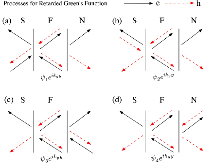
Figure 1: Schematic illustration of four types of elementary injection process for retarded Green’s function in S/F/N junctions. $e$ and $h$ denote electron and hole.

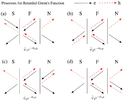
Figure 2: Schematic illustration of four types of injection process conjugate to those in Fig. 1. $e$ and $h$ denote electron and hole.

The wave functions $\psi_{1}\left(x\right)$, $\psi_{2}\left(x\right)$ $\psi_{3}\left(x\right)$, and $\psi_{4}\left(x\right)$ exhibit the processes in Figs.1(a), (b), (c) and (d), respectively and are given by

$$\psi_{1}\left(x\right) = \hat{A}_{1}e^{ik^{+}x}+a_{1}\hat{A}_{4}e^{ik^{-}x}+b_{1}\hat{A}_{3}e^{-ik^{+}x},$$ (26)

$$\psi_{2}\left(x\right) = \hat{A}_{2}e^{-ik^{-}x}+a_{2}\hat{A}_{3}e^{-ik^{+}x}+b_{2}\hat{A}_{4}e^{ik^{-}x},$$ (27)

$$\psi_{3}\left(x\right) = c_{3}\hat{A}_{3}e^{-ik^{+}x}+d_{3}\hat{A}_{4}e^{ik^{-}x},$$ (28)

$$\psi_{4}\left(x\right) = c_{4}\hat{A}_{4}e^{ik^{-}x}+d_{4}\hat{A}_{3}e^{-ik^{+}x}.$$ (29)

$\tilde{\psi}_{1}\left(x^{\prime}\right)$, $\tilde{\psi}_{2}\left(x^{\prime}\right)$, $\tilde{\psi}_{3}\left(x^{\prime}\right)$, and $\tilde{\psi}_{4}\left(x^{\prime}\right)$ exhibit those in Figs.1(a), (b), (c) and (d), respectively. They are given by

$$\tilde{\psi}_{1}\left(x^{\prime}\right) = \hat{B}_{1}e^{ik^{+}x^{\prime}}+\tilde{a}_{1}\hat{B}_{4}e^{ik^{-}x^{\prime}}+\tilde{b}_{1}\hat{B}_{3}e^{-ik^{+}x^{\prime}},$$ (30)

$$\tilde{\psi}_{2}\left(x^{\prime}\right) = \hat{B}_{2}e^{-ik^{-}x^{\prime}}+\tilde{a}_{2}\hat{B}_{3}e^{-ik^{+}x^{\prime}}+\tilde{b}_{2}\hat{B}_{4}e^{ik^{-}x^{\prime}},$$ (31)

$$\tilde{\psi}_{3}\left(x^{\prime}\right) = \tilde{c}_{3}\hat{B}_{3}e^{-ik^{+}x^{\prime}}+\tilde{d}_{3}\hat{B}_{4}e^{ik^{-}x^{\prime}},$$ (32)

$$\tilde{\psi}_{4}\left(x^{\prime}\right) = \tilde{c}_{4}\hat{B}_{4}e^{ik^{-}x^{\prime}}+\tilde{d}_{4}\hat{B}_{3}e^{-ik^{+}x^{\prime}}.$$ (33)

Substitute $\psi_{i=1\sim 4}\left(x\right)$ and $\tilde{\psi}_{i=1\sim 4}\left(x^{\prime}\right)$ into Eqs.(24) and (25), we can obtain

$$G^{R}\left(x,x^{\prime}\right)_{x>x^{\prime}}=\text{I}+\text{II}+\text{III,}$$ (34)

$$\text{I}=g_{1}\hat{A}_{1}\hat{B}_{3}^{T}e^{ik^{+}x-ik^{+}x^{\prime}}+g_{4}\hat{A}_{2}\hat{B}_{4}^{T}e^{-ik^{-}x+ik^{-}x^{\prime}},$$ (35)

$$\text{II}=g_{2}\hat{A}_{1}\hat{B}_{4}^{T}e^{ik^{+}x+ik^{-}x^{\prime}}+g_{3}\hat{A}_{2}\hat{B}_{3}^{T}e^{-ik^{-}x-ik^{+}x^{\prime}},$$ (36)

$$\begin{array}[]{c}\text{III}=g_{1}a_{1}\hat{A}_{4}\hat{B}_{3}^{T}e^{ik^{-}x-ik^{+}x^{\prime}}+g_{1}b_{1}\hat{A}_{3}\hat{B}_{3}^{T}e^{-ik^{+}x-ik^{+}x^{\prime}}\\ +g_{2}a_{1}\hat{A}_{4}\hat{B}_{4}^{T}e^{ik^{-}x+ik^{-}x^{\prime}}+g_{2}b_{1}\hat{A}_{3}\hat{B}_{4}^{T}e^{-ik^{+}x+ik^{-}x^{\prime}}\\ +g_{3}a_{2}\hat{A}_{3}\hat{B}_{3}^{T}e^{-ik^{+}x-ik^{+}x^{\prime}}+g_{3}b_{2}\hat{A}_{4}\hat{B}_{3}^{T}e^{ik^{-}x-ik^{+}x^{\prime}}\\ +g_{4}a_{2}\hat{A}_{3}\hat{B}_{4}^{T}e^{-ik^{+}x+ik^{-}x^{\prime}}+g_{4}b_{2}\hat{A}_{4}\hat{B}_{4}^{T}e^{ik^{-}x+ik^{-}x^{\prime}}\end{array},$$ (37)

and

$$G_{x<x^{\prime}}^{R}\left(x,x^{\prime}\right)=\text{I'}+\text{II'}+\text{III',}$$ (38)

I’ $$= h_{1}\hat{A}_{3}\hat{B}_{1}^{T}e^{-ik^{+}x+ik^{+}x^{\prime}}+h_{4}\hat{A}_{4}\hat{B}_{2}^{T}e^{ik^{-}x-ik^{-}x^{\prime}},$$ (39)

II’ $$= h_{2}\hat{A}_{4}\hat{B}_{1}^{T}e^{+ik^{-}x+ik^{+}x^{\prime}}+h_{3}\hat{A}_{3}\hat{B}_{2}^{T}e^{-ik^{+}x-ik^{-}x^{\prime}},$$ (40)

$$\begin{array}[]{c}\text{III'}=h_{1}\tilde{a}_{1}\hat{A}_{3}\hat{B}_{4}^{T}e^{-ik^{+}x+ik^{-}x^{\prime}}+h_{1}\tilde{b}_{1}\hat{A}_{3}\hat{B}_{3}^{T}e^{-ik^{+}x-ik^{+}x^{\prime}}\\ +h_{2}\tilde{a}_{1}\hat{A}_{4}\hat{B}_{4}^{T}e^{ik^{-}x+ik^{-}x^{\prime}}+h_{2}\tilde{b}_{1}\hat{A}_{4}\hat{B}_{3}^{T}e^{ik^{-}x-ik^{+}x^{\prime}}\\ +h_{3}\tilde{a}_{2}\hat{A}_{3}\hat{B}_{3}^{T}e^{-ik^{+}x-ik^{+}x^{\prime}}+h_{3}\tilde{b}_{2}\hat{A}_{3}\hat{B}_{4}^{T}e^{-ik^{+}x+ik^{-}x^{\prime}}\\ +h_{4}\tilde{a}_{2}\hat{A}_{4}\hat{B}_{3}^{T}e^{ik^{-}x-ik^{+}x^{\prime}}+h_{4}\tilde{b}_{2}\hat{A}_{4}\hat{B}_{4}^{T}e^{ik^{-}x+ik^{-}x^{\prime}}\end{array},$$ (41)

where we denote

$$\left\{\begin{array}[]{c}g_{1}=\alpha_{1}\tilde{c}_{3}+\alpha_{2}\tilde{d}_{4}\\ g_{2}=\alpha_{1}\tilde{d}_{3}+\alpha_{2}\tilde{c}_{4}\\ g_{3}=\alpha_{3}\tilde{c}_{3}+\alpha_{4}\tilde{d}_{4}\\ g_{4}=\alpha_{3}\tilde{d}_{3}+\alpha_{4}\tilde{c}_{4}\end{array}\right.,\left\{\begin{array}[]{c}h_{1}=\beta_{1}c_{3}+\beta_{2}d_{4}\\ h_{2}=\beta_{1}d_{3}+\beta_{2}c_{4}\\ h_{3}=\beta_{3}c_{3}+\beta_{4}d_{4}\\ h_{4}=\beta_{3}d_{3}+\beta_{4}c_{4}\end{array}\right..$$ (42)

The Green’s function must satisfy the boundary conditions obtained by integrating Eq.(14) at $x=x^{\prime}$

$$G\left(x+0,x\right)-G\left(x-0,x\right)=iv_{f}^{-1}\sigma_{y}\tau_{z}.$$ (43)

Since the right side of Eq.(43) is independent of space, we can immediately obtain II${}_{x=x^{\prime}+0}$=II’${}_{x=x^{\prime}-0}$, which gives

$$g_{2}\hat{A}_{1}\hat{B}_{4}^{T}=h_{2}\hat{A}_{4}\hat{B}_{1}^{T},$$ (44)

$$g_{3}\hat{A}_{2}\hat{B}_{3}^{T}=h_{3}\hat{A}_{3}\hat{B}_{3}^{T}.$$ (45)

By solving Eqs.(44) and (45), we can find

$$g_{2}=h_{2}=g_{3}=h_{3}=0.$$ (46)

Hence, the boundary condition becomes

$$\text{I}_{x=x^{\prime}+0}-\text{I'}_{x=x^{\prime}-0}=iv_{f}^{-1}\sigma_{y}\tau_{z}.$$ (47)

After solving this matrix equation, one can find

$$g_{1} = h_{1}=\frac{i\sqrt{Z_{1}Z_{2}}}{2v_{f}\cos\theta_{+}\left(1-\gamma^{2}\right)},$$ (48)

$$g_{4} = h_{4}=\frac{i\sqrt{Z_{1}Z_{2}}}{2v_{f}\cos\theta_{-}\left(1-\gamma^{2}\right)}.$$ (49)

The condition that III${}_{x=x^{\prime}+0}=$III’${}_{x=x^{\prime}-0}$ is guaranteed by the following detailed balanced relations,

$$g_{1}a_{1} = h_{4}\tilde{a}_{2},$$ (50)

$$g_{4}a_{2} = h_{1}\tilde{a}_{1},$$ (51)

$$g_{1}b_{1} = h_{1}\tilde{b}_{1},$$ (52)

$$g_{4}b_{2} = h_{4}\tilde{b}_{2}.$$ (53)

Thus, we have solved the retarded Green’s function

$$G_{x>x^{\prime}}^{R}\left(x,x^{\prime}\right) = g_{1}[\hat{A}_{1}\hat{B}_{3}^{T}e^{ik^{+}(x-x^{\prime})}+a_{1}\hat{A}_{4}\hat{B}_{3}^{T}e^{ik^{-}x-ik^{+}x^{\prime}}+b_{1}\hat{A}_{3}\hat{B}_{3}^{T}e^{-ik^{+}(x+x^{\prime})}]\qquad$$ (54)

$$+g_{4}[\hat{A}_{2}\hat{B}_{4}^{T}e^{-ik^{-}(x-x^{\prime})}+a_{2}\hat{A}_{3}\hat{B}_{4}^{T}e^{-ik^{+}x+ik^{-}x^{\prime}}+b_{2}\hat{A}_{4}\hat{B}_{4}^{T}e^{ik^{-}(x+x^{\prime})}],\qquad\quad$$

and

$$G_{x<x^{\prime}}^{R}\left(x,x^{\prime}\right) = h_{1}[\hat{A}_{3}\hat{B}_{1}^{T}e^{-ik^{+}(x-x^{\prime})}+\tilde{a}_{1}\hat{A}_{3}\hat{B}_{4}^{T}e^{-ik^{+}x+ik^{-}x^{\prime}}+\tilde{b}_{1}\hat{A}_{3}\hat{B}_{3}^{T}e^{-ik^{+}(x+x^{\prime})}]\qquad$$ (55)

$$+h_{4}[\hat{A}_{4}\hat{B}_{2}^{T}e^{ik^{-}(x-x^{\prime})}+\tilde{a}_{2}\hat{A}_{4}\hat{B}_{3}^{T}e^{ik^{-}x-ik^{+}x^{\prime}}+\tilde{b}_{2}\hat{A}_{4}\hat{B}_{4}^{T}e^{ik^{-}(x+x^{\prime})}].\qquad$$

3.2 Advanced Green’s function

The advanced Green’s function is analytic in the lower complex-plane $G^{A}\left(x,x^{\prime},E-i\delta\right)$. We can use incoming waves to construct it.

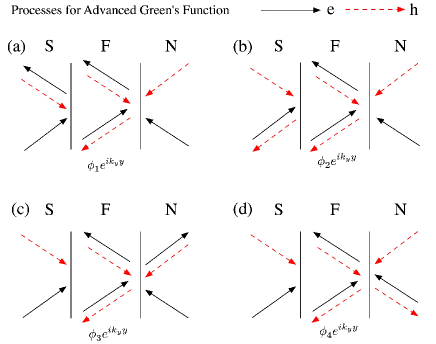
Figure 3: Schematic illustration of four types of elementary injection process for advanced Green’s function in S/F/N junctions. $e$ and $h$ denote electron and hole.

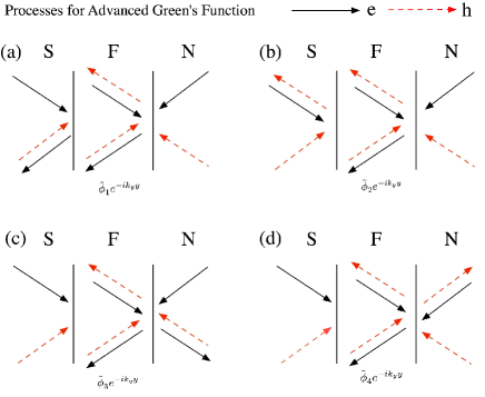
Figure 4: Schematic illustration of four types of elementary injection process conjugate to Fig.3 for advanced Green’s function in S/F/N junctions. $e$ and $h$ denote electron and hole.

The corresponding processes are shown in Figs.3 and 4. The advanced Green’s functions can be written as $G_{x>x^{\prime}}^{A}\left(x,x^{\prime},y,y^{\prime}\right)=G_{x>x^{\prime}}^{A}\left(x,x^{\prime}\right)e^{ik_{y}\left(y-y^{\prime}\right)}$ with

$$G_{x>x^{\prime}}^{A}\left(x,x^{\prime}\right)=\alpha_{1}^{\prime}\phi_{1}(x)\tilde{\phi}_{3}^{T}(x^{\prime})+\alpha_{2}^{\prime}\phi_{1}(x)\tilde{\phi}_{4}^{T}(x^{\prime})+\alpha_{3}^{\prime}\phi_{2}(x)\tilde{\phi}_{3}^{T}(x^{\prime})+\alpha_{4}^{\prime}\phi_{2}(x)\tilde{\phi}_{4}^{T}(x^{\prime}),$$ (56)

and $G_{x<x^{\prime}}^{A}\left(x,x^{\prime},y,y^{\prime}\right)=G_{x<x^{\prime}}^{A}\left(x,x^{\prime}\right)e^{ik_{y}\left(y-y^{\prime}\right)}$ with

$$G_{x<x^{\prime}}^{A}\left(x,x^{\prime}\right)=\beta_{1}^{\prime}\phi_{3}(x)\tilde{\phi}_{1}^{T}(x^{\prime})+\beta_{2}^{\prime}\phi_{4}(x)\tilde{\phi}_{1}^{T}(x^{\prime})+\beta_{3}^{\prime}\phi_{3}(x)\tilde{\phi}_{2}^{T}(x^{\prime})+\beta_{4}^{\prime}\phi_{4}(x)\tilde{\phi}_{2}^{T}(x^{\prime}).$$ (57)

In the above, $\phi_{1}(x)$, $\phi_{2}(x)$, $\phi_{3}(x)$, and $\phi_{4}(x)$ are given by

$$\phi_{1}\left(x\right) = \hat{A}_{3}e^{-ik^{+}x}+a_{1}^{\prime}\hat{A}_{2}e^{-ik^{-}x}+b_{1}^{\prime}\hat{A}_{1}e^{ik^{+}x},$$ (58)

$$\phi_{2}\left(x\right) = \hat{A}_{4}e^{ik^{-}x}+a_{2}^{\prime}\hat{A}_{1}e^{ik^{+}x}+b_{2}^{\prime}\hat{A}_{2}e^{-ik^{-}x},$$ (59)

$$\phi_{3}\left(x\right) = c_{3}^{\prime}\hat{A}_{1}e^{ik^{+}x}+d_{3}^{\prime}\hat{A}_{2}e^{-ik^{-}x},$$ (60)

$$\phi_{4}\left(x\right) = c_{4}^{\prime}\hat{A}_{2}e^{-ik^{-}x}+d_{4}^{\prime}\hat{A}_{1}e^{ik^{+}x},$$ (61)

and$\tilde{\phi}_{1}(x)$, $\tilde{\phi}_{2}(x)$, $\tilde{\phi}_{3}(x)$, and $\tilde{\phi}_{4}(x)$ are given by

$$\tilde{\phi}_{1}\left(x^{\prime}\right) = \hat{B}_{3}e^{-ik^{+}x^{\prime}}+\tilde{a}_{1}^{\prime}\hat{B}_{2}e^{-ik^{-}x^{\prime}}+\tilde{b}_{1}^{\prime}\hat{B}_{1}e^{ik^{+}x^{\prime}},$$ (62)

$$\tilde{\phi}_{2}\left(x^{\prime}\right) = \hat{B}_{4}e^{ik^{-}x^{\prime}}+\tilde{a}_{2}^{\prime}\hat{B}_{1}e^{ik^{+}x^{\prime}}+\tilde{b}_{2}^{\prime}\hat{B}_{2}e^{-ik^{-}x^{\prime}},$$ (63)

$$\tilde{\phi}_{3}\left(x^{\prime}\right) = \tilde{c}_{3}^{\prime}\hat{B}_{1}e^{ik^{+}x^{\prime}}+\tilde{d}_{3}^{\prime}\hat{B}_{2}e^{-ik^{-}x^{\prime}},$$ (64)

$$\tilde{\phi}_{4}\left(x^{\prime}\right) = \tilde{c}_{4}^{\prime}\hat{B}_{2}e^{-ik^{-}x^{\prime}}+\tilde{d}_{4}^{\prime}\hat{B}_{1}e^{ik^{+}x^{\prime}}.$$ (65)

Substitute $\phi_{i=1\sim 4}\left(x\right)$ and $\tilde{\phi}_{i=1\sim 4}\left(x^{\prime}\right)$ into Green’s function, we have

$$G_{x>x^{\prime}}^{A}\left(x,x^{\prime}\right)=\overline{\text{I}}+\overline{\text{II}}+\overline{\text{III}},$$ (66)

$$\overline{\text{I}}=g_{1}^{\prime}\hat{A}_{3}\hat{B}_{1}^{T}e^{-ik^{+}x+ik^{+}x^{\prime}}+g_{4}^{\prime}\hat{A}_{4}\hat{B}_{2}^{T}e^{ik^{-}x-ik^{-}x^{\prime}},$$ (67)

$$\overline{\text{II}}=g_{2}^{\prime}\hat{A}_{3}\hat{B}_{2}^{T}e^{-ik^{+}x-ik^{-}x^{\prime}}+g_{3}^{\prime}\hat{A}_{4}\hat{B}_{1}^{T}e^{ik^{-}x+ik^{+}x^{\prime}},$$ (68)

$$\begin{array}[]{c}\overline{\text{III}}=g_{1}^{\prime}a_{1}^{\prime}\hat{A}_{2}\hat{B}_{1}^{T}e^{-ik^{-}x+ik^{+}x^{\prime}}+g_{1}^{\prime}b_{1}^{\prime}\hat{A}_{1}\hat{B}_{1}^{T}e^{ik^{+}x+ik^{+}x^{\prime}}\\ +g_{2}^{\prime}a_{1}^{\prime}\hat{A}_{2}\hat{B}_{2}^{T}e^{-ik^{-}x-ik^{-}x^{\prime}}+g_{2}^{\prime}b_{1}^{\prime}\hat{A}_{1}\hat{B}_{2}^{T}e^{ik^{+}x-ik^{-}x^{\prime}}\\ +g_{3}^{\prime}a_{2}^{\prime}\hat{A}_{1}\hat{B}_{1}^{T}e^{ik^{+}x+ik^{+}x^{\prime}}+g_{3}^{\prime}b_{2}^{\prime}\hat{A}_{2}\hat{B}_{1}^{T}e^{-ik^{-}x+ik^{+}x^{\prime}}\\ +g_{4}^{\prime}a_{2}^{\prime}\hat{A}_{1}\hat{B}_{2}^{T}e^{ik^{+}x-ik^{-}x^{\prime}}+g_{4}^{\prime}b_{2}^{\prime}\hat{A}_{2}\hat{B}_{2}^{T}e^{-ik^{-}x-ik^{-}x^{\prime}}\end{array},$$ (69)

with

$$g_{1}^{\prime} = \alpha_{1}^{\prime}\tilde{c}_{3}^{\prime}+\alpha_{2}^{\prime}\tilde{d}_{4}^{\prime},$$ (70)

$$g_{2}^{\prime} = \alpha_{2}^{\prime}\tilde{c}_{4}^{\prime}+\alpha_{1}^{\prime}\tilde{d}_{3}^{\prime},$$ (71)

$$g_{3}^{\prime} = \alpha_{3}^{\prime}\tilde{c}_{3}^{\prime}+\alpha_{4}^{\prime}\tilde{d}_{4}^{\prime},$$ (72)

$$g_{4}^{\prime} = \alpha_{4}^{\prime}\tilde{c}_{4}^{\prime}+\alpha_{3}^{\prime}\tilde{d}_{3}^{\prime},$$ (73)

and

$$G^{A}\left(x,x^{\prime}\right)_{x<x^{\prime}}=\overline{\text{I}}\text{'}+\overline{\text{II}}\text{'}+\overline{\text{III}}\text{',}$$ (74)

$$\overline{\text{I}}\text{'}=h_{1}^{\prime}\hat{A}_{1}\hat{B}_{3}^{T}e^{ik^{+}x-ik^{+}x^{\prime}}+h_{4}^{\prime}\hat{A}_{2}\hat{B}_{4}^{T}e^{-ik^{-}x+ik^{-}x^{\prime}},$$ (75)

$$\overline{\text{II}}\text{'}=h_{2}^{\prime}\hat{A}_{2}\hat{B}_{3}^{T}e^{-ik^{-}x-ik^{+}x^{\prime}}+h_{3}^{\prime}\hat{A}_{1}\hat{B}_{4}^{T}e^{ik^{+}x+ik^{-}x^{\prime}},$$ (76)

$$\begin{array}[]{c}\overline{\text{III}}\text{'}=h_{1}^{\prime}\tilde{a}_{1}^{\prime}\hat{A}_{1}\hat{B}_{2}^{T}e^{ik^{+}x-ik^{-}x^{\prime}}+h_{1}^{\prime}\tilde{b}_{1}^{\prime}\hat{A}_{1}\hat{B}_{1}^{T}e^{ik^{+}x+ik^{+}x^{\prime}}\\ +h_{2}^{\prime}\tilde{a}_{1}^{\prime}\hat{A}_{2}\hat{B}_{2}^{T}e^{-ik^{-}x-ik^{-}x^{\prime}}+h_{2}^{\prime}\tilde{b}_{1}^{\prime}\hat{A}_{2}\hat{B}_{1}^{T}e^{-ik^{-}x+ik^{+}x^{\prime}}\\ +h_{3}^{\prime}\tilde{a}_{2}^{\prime}\hat{A}_{1}\hat{B}_{1}^{T}e^{ik^{+}x+ik^{+}x^{\prime}}+h_{3}^{\prime}\tilde{b}_{2}^{\prime}\hat{A}_{1}\hat{B}_{2}^{T}e^{ik^{+}x-ik^{-}x^{\prime}}\\ +h_{4}^{\prime}\tilde{a}_{2}^{\prime}\hat{A}_{2}\hat{B}_{1}^{T}e^{-ik^{-}x+ik^{+}x^{\prime}}+h_{4}^{\prime}\tilde{b}_{2}^{\prime}\hat{A}_{2}\hat{B}_{2}^{T}e^{-ik^{-}x-ik^{-}x^{\prime}}\end{array},$$ (77)

with

$$h_{1}^{\prime} = \beta_{1}^{\prime}c_{3}^{\prime}+\beta_{2}^{\prime}d_{4}^{\prime},$$ (78)

$$h_{2}^{\prime} = \beta_{1}^{\prime}d_{3}^{\prime}+\beta_{2}^{\prime}c_{4}^{\prime},$$ (79)

$$h_{3}^{\prime} = \beta_{3}^{\prime}c_{3}^{\prime}+\beta_{4}^{\prime}d_{4}^{\prime},$$ (80)

$$h_{4}^{\prime} = \beta_{3}^{\prime}d_{3}^{\prime}+\beta_{4}^{\prime}c_{4}^{\prime}.$$ (81)

The boundary conditions of Green’s function becomes,

$$G\left(x+0,x\right)-G\left(x-0,x\right)=iv_{f}^{-1}\sigma_{y}\tau_{z}.$$ (82)

Following the same procedure as in the case of calculating retarded Green’s function, we can find

$$g_{1}^{\prime} = h_{1}^{\prime}=\frac{i\sqrt{Z_{1}Z_{2}}}{2v_{f}\cos\theta_{+}\left[\gamma^{2}-1\right]},$$ (83)

$$g_{2}^{\prime} = h_{2}^{\prime}=g_{3}^{\prime}=h_{3}^{\prime}=0,$$ (84)

$$g_{4}^{\prime} = h_{4}^{\prime}=\frac{i\sqrt{Z_{1}Z_{2}}}{2v_{f}\cos\theta_{-}\left[\gamma^{2}-1\right]}.$$ (85)

The detailed balanced relations are given by

$$g_{1}^{\prime}a_{1}^{\prime} = h_{4}^{\prime}\tilde{a}_{2}^{\prime},$$ (86)

$$g_{4}^{\prime}a_{2}^{\prime} = h_{1}^{\prime}\tilde{a}_{1}^{\prime},$$ (87)

$$g_{1}^{\prime}b_{1}^{\prime} = h_{1}^{\prime}\tilde{b}_{1}^{\prime},$$ (88)

$$g_{4}^{\prime}b_{2}^{\prime} = h_{4}^{\prime}\tilde{b}_{2}^{\prime}.$$ (89)

Then, the advanced Green’s function is obtained by

$$G_{x>x^{\prime}}^{A}\left(x,x^{\prime}\right) = g_{1}^{\prime}[\hat{A}_{3}\hat{B}_{1}^{T}e^{-ik^{+}(x-x^{\prime})}+a_{1}^{\prime}\hat{A}_{2}\hat{B}_{1}^{T}e^{-ik^{-}x+ik^{+}x^{\prime}}+b_{1}^{\prime}\hat{A}_{1}\hat{B}_{1}^{T}e^{ik^{+}(x+x^{\prime})}]\qquad$$ (90)

$$+g_{4}^{\prime}[\hat{A}_{4}\hat{B}_{2}^{T}e^{ik^{-}(x-x^{\prime})}+a_{2}^{\prime}\hat{A}_{1}\hat{B}_{2}^{T}e^{ik^{+}x-ik^{-}x^{\prime}}+b_{2}^{\prime}\hat{A}_{2}\hat{B}_{2}^{T}e^{-ik^{-}(x+x^{\prime})}],\quad\quad\quad$$

and

$$G_{x<x^{\prime}}^{A}\left(x,x^{\prime}\right) = h_{1}^{\prime}[\hat{A}_{1}\hat{B}_{3}^{T}e^{ik^{+}(x-x^{\prime})}+\tilde{a}_{1}^{\prime}\hat{A}_{1}\hat{B}_{2}^{T}e^{ik^{+}x-ik^{-}x^{\prime}}+\tilde{b}_{1}^{\prime}\hat{A}_{1}\hat{B}_{1}^{T}e^{ik^{+}(x+x^{\prime})}]\qquad$$ (91)

$$+h_{4}^{\prime}[\hat{A}_{2}\hat{B}_{4}^{T}e^{-ik^{-}(x-x^{\prime})}+\tilde{a}_{2}^{\prime}\hat{A}_{2}\hat{B}_{1}^{T}e^{-ik^{-}x+ik^{+}x^{\prime}}+\tilde{b}_{2}^{\prime}\hat{A}_{2}\hat{B}_{2}^{T}e^{-ik^{-}(x+x^{\prime})}].\qquad\quad$$

3.3 Numerical Results

We first focus on the local density of states (LDOS) $\rho$ on the edge of superconductor $x=0$. Here, $\rho$ is given by

$$\rho=-\frac{1}{\pi}\mathrm{Im}\left[G_{11}^{R}\left(x,x\right)+G_{22}^{R}\left(x,x\right)\right].$$ (92)

The obtained results are shown in Fig.5. There are resonant states inside the gap when the magnetization is along $x$- or $z$-axis. If resonant states are located at zero energy, they are called Majorana Fermions. We can see when the magnetization is along $x$-axis, the LDOS is highly asymmetric with respect to zero energy, as shown in Fig.5(a). This reveals that the in-gap resonant states have the characteristic similar to Shiba states, $i.e.,$ magnetic impurity state coupled to superconductor, in spin non-degenerate system realized on the surface of TI [19, 20, 21, 22]. The LDOS becomes more prominent and symmetric when the magnetization is along $z$-axis, as shown in Fig.5(b). These results are consistent with previous theories of Majorana fermion on TI and its tunneling effect [23, 24].

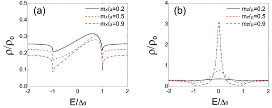
Figure 5: Local density of states at $x=0$ in S/F/N junction. (a) $m_{x}/\mu=0.2$, $0.5,$ and $0.9$ and (b) $m_{z}/\mu=0.2$, $0.5,$ and $0.9$. $\rho_{0}$ denotes the local density of states of bulk normal metal at Fermi energy. Other parameters are set as $\Delta_{0}/\mu=0.001$ and $\mu L/v_{f}=2$.

Next, we look at the pair amplitude. We obtain the Matsubara Green’s function by analytical continuation,

$$G^{R}\left(E+i\delta\right) \rightarrow G\left(i\left|\omega_{n}\right|\right),$$ (93)

$$G^{A}\left(E-i\delta\right) \rightarrow G\left(-i\left|\omega_{n}\right|\right).$$ (94)

Then, we write down the Matsubara Green’s function explicitly

$$G=\left[\begin{array}[]{cccc}G_{\uparrow\uparrow}&G_{\uparrow\downarrow}&F_{\uparrow\uparrow}&F_{\uparrow\downarrow}\\ G_{\downarrow\uparrow}&G_{\downarrow\downarrow}&F_{\downarrow\uparrow}&F_{\downarrow\downarrow}\\ \breve{F}_{\uparrow\uparrow}&\breve{F}_{\uparrow\downarrow}&\breve{G}_{\uparrow\uparrow}&\breve{G}_{\uparrow\downarrow}\\ \breve{F}_{\downarrow\uparrow}&\breve{F}_{\downarrow\downarrow}&\breve{G}_{\downarrow\uparrow}&\breve{G}_{\downarrow\downarrow}\end{array}\right],$$ (95)

The pair amplitudes at $x=x^{\prime}<0$ are given by

$$F_{\uparrow\uparrow}^{odd} = \frac{\breve{F}_{\uparrow\uparrow}\left(\omega_{n},x,x\right)-\breve{F}_{\uparrow\uparrow}\left(-\omega_{n},x,x\right)}{2},$$ (96)

$$F_{\uparrow\downarrow}^{odd} = \frac{\breve{F}_{\uparrow\downarrow}\left(\omega_{n},x,x\right)-\breve{F}_{\uparrow\downarrow}\left(-\omega_{n},x,x\right)}{2},$$ (97)

$$F_{\downarrow\uparrow}^{odd} = \frac{\breve{F}_{\downarrow\uparrow}\left(\omega_{n},x,x\right)-\breve{F}_{\downarrow\uparrow}\left(-\omega_{n},x,x\right)}{2},$$ (98)

$$F_{\downarrow\downarrow}^{odd} = \frac{\breve{F}_{\downarrow\downarrow}\left(\omega_{n},x,x\right)-\breve{F}_{\downarrow\downarrow}\left(-\omega_{n},x,x\right)}{2},\quad$$ (99)

$$F_{\uparrow\uparrow}^{even} = \frac{\breve{F}_{\uparrow\uparrow}\left(\omega_{n},x,x\right)+\breve{F}_{\uparrow\uparrow}\left(-\omega_{n},x,x\right)}{2},$$ (100)

$$F_{\uparrow\downarrow}^{even} = \frac{\breve{F}_{\uparrow\downarrow}\left(\omega_{n},x,x\right)+\breve{F}_{\uparrow\downarrow}\left(-\omega_{n},x,x\right)}{2},$$ (101)

$$F_{\downarrow\uparrow}^{even} = \frac{\breve{F}_{\downarrow\uparrow}\left(\omega_{n},x,x\right)+\breve{F}_{\downarrow\uparrow}\left(-\omega_{n},x,x\right)}{2},$$ (102)

$$F_{\downarrow\downarrow}^{even} = \frac{\breve{F}_{\downarrow\downarrow}\left(\omega_{n},x,x\right)+\breve{F}_{\downarrow\downarrow}\left(-\omega_{n},x,x\right)}{2}.\quad$$ (103)

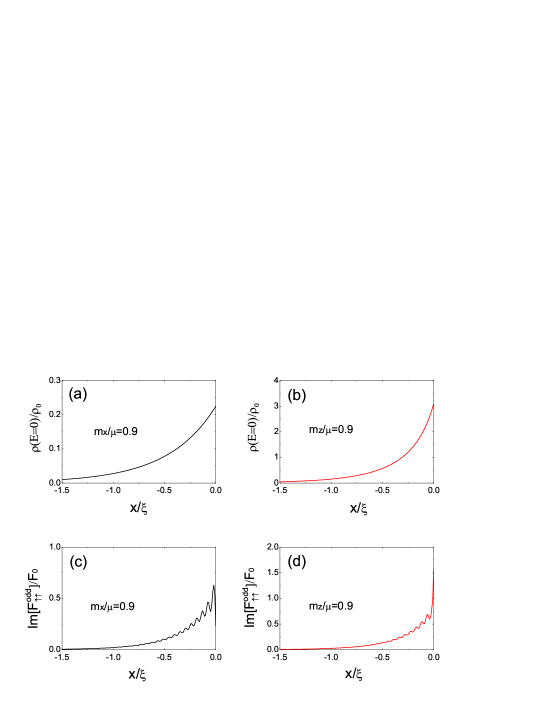
Figure 6: Spatial dependence of zero energy local density of states, $i.e.$, the LDOS in the S side in S/F/N junction for magnetization along (a) $x$-axis and (b)$z$-axis. The spatial dependence of $F_{\uparrow\uparrow}^{odd}$ is shown in (c) and (d) corresponding to (a) and (b), respectively. $F_{0}$ is the bulk value of $F_{\uparrow\downarrow}^{even}$ in S. Other parameters are set as the same as in Fig. 5.

We calculate the spatial dependence of the odd-frequency pair amplitude $F_{\uparrow\uparrow}^{odd}$. It is known that odd-frequency pairing is generated by spin-rotational symmetry breaking or translational symmetry breaking [25, 26]. The magnitude of odd-frequency pair amplitude is hugely enhanced in the presence of zero energy Andreev bound state [26] and induces anomalous proximity effect [27]. It is a remarkable feature that Majorana fermion always accompanies odd-frequency pairing [28, 29]. Thus, it is quite interesting to compare the relation between LDOS and odd-frequency pairing. Among various symmetries of odd-frequency pairings, we focus on the odd-frequency $s$-wave pairing. We show the results in Fig.6. It is shown that $F_{\uparrow\uparrow}^{odd}$ is enhanced near the S/F interface and there is a one to one correspondence between odd-frequency pairing and Majorana fermion. The results demonstrate the simultaneous penetration of Majorana fermions and odd-frequency pairing into superconducting region.

4 Josephson Current in S/F/S junction on TI surface

In this section, we derive a Josephson current. We treat S/F/S junction where the left S side is chosen as the same as that in the previous section. The phase difference between the left and right S side is $\varphi$ so that the pair potential in the right S is given by $\Delta e^{-i\varphi}$. The derivation of the Josephson current is performed in the left S side. We start from the continuity equation[30]

$$\frac{\partial}{\partial t}\hat{\rho}+\partial_{x}\hat{J}_{x}+\hat{S}=0,$$ (104)

with

$$\hat{\rho}=-e\left(\hat{\Psi}_{\uparrow}^{{\dagger}}\hat{\Psi}_{\uparrow}+\hat{\Psi}_{\downarrow}^{{\dagger}}\hat{\Psi}_{\downarrow}\right),$$ (105)

$$\hat{J}_{x}=eiv_{f}\left[\hat{\Psi}_{\downarrow}^{{\dagger}}\hat{\Psi}_{\uparrow}-\hat{\Psi}_{\uparrow}^{{\dagger}}\hat{\Psi}_{\downarrow}\right],$$ (106)

and

$$\hat{S}=ie\Delta\left[\hat{\Psi}_{\downarrow}\hat{\Psi}_{\uparrow}-\hat{\Psi}_{\uparrow}^{{\dagger}}\hat{\Psi}_{\downarrow}^{{\dagger}}-\hat{\Psi}_{\uparrow}\hat{\Psi}_{\downarrow}+\hat{\Psi}_{\downarrow}^{{\dagger}}\hat{\Psi}_{\uparrow}^{{\dagger}}\right].$$ (107)

Then, we make the wick rotation so that the time becomes imaginary $t\rightarrow i\tau$. The operators can be expressed by Matsubara Green’s function as

$$\left\langle{{\hat{J}_{x}}}\right\rangle {=} \frac{iev_{f}}{2}{{\underset{{}_{\begin{subarray}{c}x\rightarrow x^{\prime}\\ \tau^{\prime}\rightarrow\tau+0^{+}\end{subarray}}}{\lim}}}\left\langle{{\hat{\Psi}_{\downarrow}^{{\dagger}}(x^{\prime}\tau^{\prime})\hat{\Psi}_{\uparrow}(x\tau)-\hat{\Psi}_{\uparrow}^{{\dagger}}(x^{\prime}\tau^{\prime})\hat{\Psi}_{\downarrow}(x\tau)-\hat{\Psi}_{\uparrow}(x^{\prime}\tau^{\prime})\hat{\Psi}_{\downarrow}^{{\dagger}}(x\tau)+\hat{\Psi}_{\downarrow}(x^{\prime}\tau^{\prime})\hat{\Psi}_{\uparrow}^{{\dagger}}(x\tau)}}\right\rangle$$ (108)

$$= \frac{iev_{f}}{2}{\underset{{}_{\begin{subarray}{c}x\rightarrow x^{\prime}\\ \tau^{\prime}\rightarrow\tau+0^{+}\end{subarray}}}{\lim}[G_{12}(x\tau,x^{\prime}\tau^{\prime})-G_{21}(x\tau,x^{\prime}\tau^{\prime})+G_{34}(x\tau,x^{\prime}\tau^{\prime})-G_{43}(x\tau,x^{\prime}\tau^{\prime})],}$$

$$\left\langle\hat{S}\right\rangle = ie\Delta\underset{{}_{\begin{subarray}{c}x\rightarrow x^{\prime}\\ \tau^{\prime}\rightarrow\tau+0^{+}\end{subarray}}}{\lim}\left\langle\Psi_{\downarrow}\left(x^{\prime}\tau^{\prime}\right)\Psi_{\uparrow}\left(x\tau\right)-\Psi_{\uparrow}^{{\dagger}}\left(x^{\prime}\tau^{\prime}\right)\Psi_{\downarrow}^{{\dagger}}\left(x\tau\right)-\Psi_{\uparrow}\left(x^{\prime}\tau^{\prime}\right)\Psi_{\downarrow}\left(x\tau\right)+\Psi_{\downarrow}^{{\dagger}}\left(x^{\prime}\tau^{\prime}\right)\Psi_{\uparrow}^{{\dagger}}\left(x\tau\right)\right\rangle$$ (109)

$$= ie\Delta\underset{{}_{\begin{subarray}{c}x\rightarrow x^{\prime}\\ \tau^{\prime}\rightarrow\tau+0^{+}\end{subarray}}}{\lim}[G_{14}\left(x\tau,x^{\prime}\tau^{\prime}\right)-G_{23}\left(x\tau,x^{\prime}\tau^{\prime}\right)+G_{32}\left(x\tau,x^{\prime}\tau^{\prime}\right)-G_{41}\left(x\tau,x^{\prime}\tau^{\prime}\right)].$$

For the positive frequency $\omega_{n}>0$, we can obtain the Matsubara Green’s function by analytical continuation $E+i\delta\rightarrow i\omega_{n}$ from the retarded Green’s function

$$G_{x>x^{\prime}}^{R}\left(x,x^{\prime}\right) = g_{1}\left[\hat{A}_{1}\hat{B}_{3}^{T}e^{ik^{+}(x-x^{\prime})}+a_{1}\hat{A}_{4}\hat{B}_{3}^{T}e^{ik^{-}x-ik^{+}x^{\prime}}+b_{1}\hat{A}_{3}\hat{B}_{3}^{T}e^{-ik^{+}(x+x^{\prime})}\right]$$ (110)

$$+g_{4}\left[\hat{A}_{2}\hat{B}_{4}^{T}e^{-ik^{-}(x-x^{\prime})}+a_{2}\hat{A}_{3}\hat{B}_{4}^{T}e^{-ik^{+}x+ik^{-}x^{\prime}}+b_{2}\hat{A}_{4}\hat{B}_{4}^{T}e^{ik^{-}(x+x^{\prime})}\right].\qquad$$

We can find

$$\left\langle\hat{J}_{x}\right\rangle=ev_{f}\left[\frac{g_{1}a_{1}}{Z_{2}}(e^{-i\theta_{+}}+e^{i\theta_{-}})-\frac{g_{4}a_{2}}{Z_{1}}(e^{i\theta_{+}}+e^{-i\theta_{-}})\right]\gamma e^{i\left(k^{-}-k^{+}\right)x}.$$ (111)

It is noted that

$$k^{+} = \sqrt{\left(\mu+i\sqrt{\omega_{n}^{2}+\Delta^{2}}\right)^{2}-k_{y}^{2}}/v_{f},$$ (112)

$$k^{-} = \sqrt{\left(\mu-i\sqrt{\omega_{n}^{2}+\Delta^{2}}\right)^{2}-k_{y}^{2}}/v_{f},$$ (113)

we have the relations

$$k^{+2}-k^{-2}=4ik_{f}\sqrt{\omega_{n}^{2}+\Delta^{2}}/v_{f},\quad\quad\left(\mu/v_{f}=k_{f}\right),$$ (114)

and

$$e^{-i\theta_{+}}+e^{i\theta_{-}} = \frac{1}{4}\frac{k^{+}+k^{-}}{k_{f}}Z_{2},$$ (115)

$$e^{i\theta_{+}}+e^{-i\theta_{-}} = \frac{1}{4}\frac{k^{+}+k^{-}}{k_{f}}Z_{1}.$$ (116)

Hence, quasiparticle current becomes

$$\left\langle\hat{J}_{x}\right\rangle=\frac{e\sqrt{Z_{1}Z_{2}}\left(k^{+}+k^{-}\right)\Delta}{16\sqrt{\omega_{n}^{2}+\Delta^{2}}}\left[\frac{a_{1}}{k_{f}\cos\theta_{+}}-\frac{a_{2}}{k_{f}\cos\theta_{-}}\right]e^{i\left(k^{-}-k^{+}\right)x}.$$ (117)

The current which arises from the source term is given by

$$J_{s} = \int_{0}^{x}dx\left\langle\hat{S}\right\rangle=ei\Delta\left[-g_{1}a_{1}+g_{4}a_{2}\right]\frac{\left(\gamma^{2}-1\right)}{2}\int_{0}^{x}dx\left[e^{i\left(k^{-}-k^{+}\right)x}\right]$$ (118)

$$= \frac{e\sqrt{Z_{1}Z_{2}}\left(k^{+}+k^{-}\right)\Delta}{16\sqrt{\omega_{n}^{2}+\Delta^{2}}}\left[\frac{a_{1}}{k_{f}\cos\theta_{+}}-\frac{a_{2}}{k_{f}\cos\theta_{-}}\right]\left[1-e^{i\left(k^{-}-k^{+}\right)x}\right].$$

Finally, we can obtain the total Josephson current $J=\left\langle\hat{J}_{x}\right\rangle+J_{s}$

$$J=\frac{e\sqrt{Z_{1}Z_{2}}\left(k^{+}+k^{-}\right)\Delta}{16\sqrt{\omega_{n}^{2}+\Delta^{2}}}\left[\frac{a_{1}}{k_{f}\cos\theta_{+}}-\frac{a_{2}}{k_{f}\cos\theta_{-}}\right],(\omega_{n}>0).$$ (119)

In the same way, we obtain the Josephson current for the negative frequency region from the analytical continuation from advanced Green’s function

$$J=\frac{-e\sqrt{Z_{1}Z_{2}}\left(k^{+}+k^{-}\right)\Delta}{16\sqrt{\omega_{n}^{2}+\Delta^{2}}}\left[\frac{a_{1}^{\prime}}{k_{f}\cos\theta_{+}}-\frac{a_{2}^{\prime}}{k_{f}\cos\theta_{-}}\right],(\omega_{n}<0).$$ (120)

We sum Matsubara frequencies and wave vector $k_{y}$. Then, we obtain the Josephson current

$$I = ek_{B}T\sum_{k_{y},\omega_{n}>0}\frac{\sqrt{Z_{1}Z_{2}}\left(k^{+}+k^{-}\right)\Delta}{16\sqrt{\omega_{n}^{2}+\Delta^{2}}}\left[\frac{a_{1}}{k_{f}\cos\theta_{+}}-\frac{a_{2}}{k_{f}\cos\theta_{-}}\right]$$ (121)

$$+\sum_{k_{y},\omega_{n}<0}\frac{-\sqrt{Z_{1}Z_{2}}\left(k^{+}+k^{-}\right)\Delta}{16\sqrt{\omega_{n}^{2}+\Delta^{2}}}\left[\frac{a_{1}^{\prime}}{k_{f}\cos\theta_{+}}-\frac{a_{2}^{\prime}}{k_{f}\cos\theta_{-}}\right].$$

The above equation is an extended version of Furusaki-Tsukada’s formula for Josephson current on TI surface. The physical picture is that the Josephson current is carried via Andreev reflection which transfers (annihilates) Cooper pair. In the quasiclassical limit, with $E$, $\Delta\ll\mu$, we have

$$\begin{array}[]{l}Z_{1}\approx Z_{2}\approx 2,\\ \theta_{+}\approx\theta_{-}\approx\theta,\\ k_{+}\approx k_{-}\approx k_{f}\cos\theta.\end{array}$$ (122)

Then, the resulting Josephson current becomes

$$I=\frac{ek_{B}T\Delta}{2}\sum_{k_{y}}\left[\sum_{\omega_{n}>0}\frac{(a_{1}-a_{2})}{\sqrt{\omega_{n}^{2}+\Delta^{2}}}+\sum_{\omega_{n}<0}-\frac{(a_{1}^{\prime}-a_{2}^{\prime})}{\sqrt{\omega_{n}^{2}+\Delta^{2}}}\right].$$ (123)

We can derive that the contribution from negative frequencies are the same as that from positive frequencies in the above equation. Then we have

$$I=ek_{B}T\Delta\sum_{k_{y},\omega_{n}>0}\frac{(a_{1}-a_{2})}{\sqrt{\omega_{n}^{2}+\Delta^{2}}}.$$ (124)

In Fig.7, we present results of Josephson current in S/F/S junctions on TI surface. It is normalized by $eR_{N}I/\Delta_{0}$ where $R_{N}$ is the resistivity of the junction in normal state and $\Delta_{0}=\Delta(T=0)$. In panels (a) and (b), we plot Josephson current $I(\varphi)$ as a function of the phase difference $\varphi$. We can see that $I(\varphi)$ has a dominant first order $\sin\varphi$ coupling in both cases independent of the direction of the magnetization. We also plot the maximum Josephson current $I_{c}$ with respect to $\varphi$. Here, we assume that the temperature dependence of pair potential $\Delta$ obeys the BCS relation: $\Delta=\Delta_{0}\tanh(1.74\sqrt{T_{c}/T-1})$ with $\Delta_{0}=1.76k_{B}T_{c}$ where $T_{c}$ is the critical temperature.

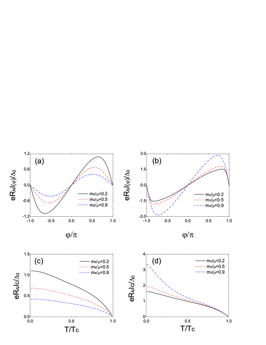
Figure 7: Josephson current in S/F/S junction on TI surface. Current phase relation for (a) magnetization along $x$-axis and (b) that along $z$-axis. Temperature is set to be $T=0.1T_{c}$ where $T_{c}$ is the critical temperature. The maximum Josephson current for magnetization along $x$- and $z$-axis is shown in (c) and (d), respectively. Other parameters are set as the same as in Fig.6.

We plot $I_{C}$ as a function of temperature in panels (c) and (d). The magnitude of $eR_{N}I_{C}/\Delta_{0}$ is enhanced with the increase of the magnetization along $z$-axis shown in panel (d), while it becomes suppressed as the magnitude of magnetization along $x$-axis increases, as shown in panel (c). In the low temperature region, the temperature dependence of $I_{c}$ is seriously influenced by the presence of zero-energy states. When the magnetization is along $x$-axis, $I_{c}$ has the Ambegaokar-Baratoff[31] type temperature dependence for low transmissivity junction due to the absence of zero-energy states. It is consistent with the energy dependence of LDOS as shown in panel (a). Although Shiba state exists at the interface, the peak of LDOS is not located at zero energy. Then, Shiba state does not contribute to the enhancement of Josephson current at low temperatures. When the magnetization is along $z$-axis, the significant enhancement of the magnitude of LDOS at zero energy by Majorana fermion gives rise to the Kulik-Omelyanchuk[32] type behavior of $I_{c}$, i.e. the dash dotted line in panel (b). Also, as compared to Fig.5, we can find that the magnitude of $I_{c}$ increases (or decreases) as the zero energy states is enhanced (or suppressed).

5 Discussion and Conclusion

In this article, we have shown how to construct Green’s function in superconducting hybrid systems on the surface of topological insulator following McMillan’s formalism where the energy spectrum of electrons obeys linear dispersion. We have obtained not only retarded Green’s function but also advanced one. We have applied this theory for a model of superconductor/ferromagnet/normal metal (S/F/N) junction. When the magnetization is along $x$-axis, the local density of states is highly asymmetric around zero energy. On the other hand, when the magnetization is along $z$-axis, we have obtained a prominent zero-energy peak due to the generation of Majorana fermion. At the same time, pair amplitude of odd frequency pairing is also enhanced. We have also derived an extended Furusaki-Tsukada’s formula of d.c. Josephson current in S/F/S junctions. It is remarkable that a compact formula of Josephson current is obtained. When the magnetization is along $x$-axis, $I_{c}$ has the Ambegaokar-Baratoff type temperature dependence for low transmissivity junction. On the other hand, when the magnetization is along the $z$-axis, we can obtain Kulik-Omelyanchuk type behavior of $I_{c}$ due to the presence of prominent zero-energy states by Majorana fermion.

Before closing this article, we mention about the relation between the present theory and the quasiclassical Green’s function theory. It is an efficient way to study proximity effect based on quasiclassical Green’s function theory as far as we are focusing on the low energy excitation. Although there have been many good review articles of quasiclassical Green’s function theory [33, 34, 35, 36], a theoretical procedure to formulate quasiclassical Green’s function in superconducting junctions on TI has not been fully clarified yet[37]. Only the case in Graphene junctions has been studied up to now [38, 39]. Thus, it is promising to start from our obtained Green’s function to establish the quasiclassical theory of TI-based junctions and compare with the present results in our article in future.

This work has been supported by Topological Materials Science (TMS) (No. 15H05853) and No. 25287085 from the Ministry of Education, Culture, Sports, Science, and Technology, Japan (MEXT), and by the Core Research for Evolutional Science and Technology (CREST) of the Japan Science and Technology Corporation (JST).

We thank P. Burset, K. Yada, A.A.Golubov and Y. Asano for valuable discussions.

References

- [1] W. L. McMillan, Phys. Rev. 175, 559 (1968).
- [2] M. P. Samanta and S. Datta, Phys. Rev. B 57, 10972 (1998).
- [3] A. Furusaki, Physica (Amsterdam) 203B, 214 (1994).
- [4] G. E. Blonder, M. Tinkham, and T. M. Klapwijk, Phys. Rev. B 25, 4515 (1982).
- [5] P. G. De Gennes, "Superconductivity of Metals and Alloys", Benjamin, New York (1966).
- [6] A. Furusaki and M. Tsukada, Solid State Commun. 78, 299 (1991).
- [7] S. Kashiwaya and Y. Tanaka, Rep. Prog. Phys. 63, 1641 (2000).
- [8] Y. Tanaka and S. Kashiwaya, Phys. Rev. B 53, R11957 (1996).
- [9] Y. Tanaka and S. Kashiwaya, Phys. Rev. B 56,892 (1997).
- [10] Yu.S. Barash, H. Burkhardt, D. Rainer, Phys. Rev. Lett. 77, 4070 (1996).
- [11] Y. Asano, Phys. Rev. B 64, 224515 (2001).
- [12] Y. Asano, Phys. Rev. B 74, R220501 (2006).
- [13] P. M. R. Brydon, D. Manske and M. Sigrist, J. Phys. Soc. Jpn. 77, 103714 (2008).
- [14] Y. Asano, T. Yoshida, Y. Tanaka, and A. A. Golubov, Phys. Rev. B 78, 014514 (2008).
- [15] W. J. Herrera, P. Burset, and A. L. Yeyati, J. Phys.: Condens. Matter 22, 275304 (2010).
- [16] F. Crépin, Pablo Burset and B. Trauzettel, preprint, arxiv:1503.07784 (2015).
- [17] C. Benjamin, Europhys. Lett. 110, 50003 (2015).
- [18] C. X. Bai and Y.L. Yang, Nanoscale Research Letters 9, 515(2014).
- [19] L. Yu, Acta Phys. Sin. 21, 75 (1965).
- [20] H. Shiba, Prog. Theor. Phys. 40, 435 (1968).
- [21] A. I. Rusinov, Sov. Phys. JETP Lett. 29, 1101 (1969).
- [22] B. Lu, P. Burset, K. Yada, and Y. Tanaka, preprint, arXiv:1504.06208 (2015) (accepted for publication on Supercond. Sci. Technol.).
- [23] L. Fu and C. L. Kane, Phys. Rev. Lett. 100, 096407 (2008).
- [24] Y. Tanaka, T. Yokoyama, and N. Nagaosa, Phys. Rev. Lett. 103, 107002 (2009).
- [25] F. S. Bergeret, A. F. Volkov, and K. B. Efetov, Phys. Rev. Lett. 86, 4096 (2001); F. S. Bergeret, A. F. Volkov, and K. B. Efetov, Rev. Mod. Phys. 77, 1321 (2005).
- [26] Y. Tanaka, M. Sato, and N. Nagaosa, J. Phys. Soc. Jpn. 81, 011013 (2012).
- [27] Y. Tanaka and A. A. Golubov, Phys. Rev. Lett. 98, 037003 (2007).
- [28] Y. Asano and Y. Tanaka, Phys. Rev. B 87, 104513 (2013).
- [29] H. Ebisu, K. Yada, H. Kasai, and Y. Tanaka, Phys. Rev. B 91, 054518 (2015).
- [30] We do not consider the current since we can prove that in our setup.
- [31] V. Ambegaokar and A. Baratoff, Phys. Rev. Lett. 10,486 (1963); 11, 104 (1963).
- [32] I. O. Kulik and A. N. Omelyanchuk, Fiz. Nizk. Temp. 4, 296 (1978)[Sov. J. Low Temp. Phys. 4, 142 (1978)].
- [33] J.W. Serene and D. Rainer, Phys. Rep. 101, 221 (1983).
- [34] W. Belzig, F. K. Wilhelm, C. Bruder, G. Schon and A. Zaikin, Superlattices Microstruct. 25, 1251 (1999).
- [35] M. Eschrig, Phys. Rev. B 61, 9061 (2000).
- [36] N. Kopnin, “Theory of Nonequilibrium Superconductivity”, Clarendon Press, Oxford (2001).
- [37] After the submission of the present paper, we notice the work “A. Zyuzin, M. Alidoust, and D. Loss, Arxiv: 1511.01486(2015)”, where the Usadel approach for Josephson effect in a S-TI-S junction is discussed.
- [38] Y. Takane and K.-I. Imura, J. Phys. Soc. Jpn. 80, 043702 (2011).
- [39] A. Ossipov, M. Titov, and C. W. J. Beenakker, Phys. Rev. B 75, R241401 (2007).