Dengue disease: a multiobjective viewpoint

Abstract.

During the last decades, the global prevalence of dengue progressed dramatically. It is a disease that is now endemic in more than one hundred countries of Africa, America, Asia, and the Western Pacific. In this paper, we present a mathematical model for the dengue disease transmission described by a system of ordinary differential equations and propose a multiobjective approach to find the most effective ways of controlling the disease. We use evolutionary multiobjective optimization (EMO) algorithms to solve the resulting optimization problem, providing the performance comparison of different algorithms. The obtained results show that the multiobjective approach is an effective tool to solve the problem, giving higher quality and wider range of solutions compared to the traditional technique. The obtained trade-offs provide a valuable information about the dynamics of infection transmissions and can be used as an input in the process of planning the intervention measures by the health authorities. Additionally, a suggested hybrid EMO algorithm produces highly superior performance compared to five other state-of-the-art EMO algorithms, being indispensable to efficiently optimize the proposed model.

1. Introduction

Epidemiology – the study of patterns of diseases including those which are noncommunicable infections in population – has become more relevant and indispensable in the development of new models and explanations for the outbreaks, namely due to their propagation and causes. In epidemiology, an infection is said to be endemic in a population when it is maintained in the population without the need for external inputs. An epidemic occurs when new cases of a certain disease appears, in a given human population during a given period, and then essentially disappears.

Mathematical modeling is critical to understand how epidemiological diseases spread. It can help to explain the nature and dynamics of infection transmissions and can be used to devise effective strategies for fighting them. When formulating a model for a particular disease, we should make a trade-off between simple models – that omit several details and generally are used for specific situations in a short time, but have the disadvantage of possibly being naive and unrealistic – and more complex models, with more details and more realistic, but generally more difficult to solve or could contain parameters which their estimates cannot be obtained.

Dengue is a vector-borne disease transmitted from an infected human to a female Aedes mosquito by a bite. Then, the mosquito, that needs regular meals of blood to feed their eggs, bites a potentially healthy human and transmits the disease, turning it into a cycle.

There are four distinct, but closely related, viruses that cause dengue. The four serotypes, named DEN-1 to DEN-4, belong to the Flavivirus family, but they are antigenically distinct. Recovery from infection by one virus provides lifelong immunity against that virus but provides only partial and transient protection against subsequent infection by the other three viruses. There are strong evidences that a sequential infection increases the risk of developing dengue hemorrhagic fever.

The spread of dengue is attributed to the geographic expansion of the mosquitoes responsible for the disease: Aedes aegypti and Aedes albopictus. The Aedes aegypti mosquito is a tropical and subtropical species widely distributed around the world, mostly between latitudes $35^{o}$N and 35^oS. In urban areas, Aedes mosquitoes breed on water collections in artificial containers such as cans, plastic cups, used tires, broken bottles and flower pots. Due to its high interaction with humans and its urban behavior, the Aedes aegypti mosquito is considered the major responsible for the dengue transmission.

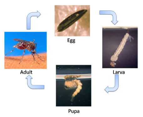
Figure 1. Life cycle of Aedes aegypti.

The life cycle of a mosquito has four distinct stages: egg, larva, pupa and adult, as it is possible to see in Figure 1. In the case of Aedes aegypti, the first three stages take place in, or near, the water, whereas the air is the medium for the adult stage [20].

It is very difficult to control or eliminate Aedes aegypti mosquitoes due to their resiliency, fast adaptation to changes in the environment and their ability to rapidly bounce back to initial numbers after disturbances resulting from natural phenomena (e.g., droughts) or human interventions (e.g., control measures).

Primary prevention of dengue resides mainly in mosquito control. There are two primary methods: larval control and adult mosquito control, depending on the intended target. Larvicide treatment is done through long-lasting chemical in order to kill larvae and preferably have World Health Organization clearance for use in drinking water [8]. Adulticides is the most common measure. Its application can have a powerful impact on the abundance of adult mosquito vector. However, the efficacy is often constrained by the difficulty in achieving sufficiently high coverage of resting surfaces [9].

In this paper, our first motivation is to analyse a mathematical model for the dengue disease transmission, including the control parameter representing measures to fight the disease. Since there are different goals that can be sought dealing with the dengue epidemic, we suggest a multiobjective approach to find the optimal control in the proposed model. Such approach better reflects the nature of an underlying decision-making problem, hence, can provide more interesting results.

Without loss of generality, a multiobjective optimization (MO) problem with $m$ objectives and $n$ decision variables can be mathematically formulated as follows:

$$\begin{array}[]{rl}\text{minimize:}&\boldsymbol{f}(\boldsymbol{x})=(f_{1}(\boldsymbol{x}),f_{2}(\boldsymbol{x}),\ldots,f_{m}(\boldsymbol{x}))^{\text{T}}\\ \text{subject to:}&\boldsymbol{x}\in\Omega,\end{array}$$ (1.1)

where $\boldsymbol{x}$ is the decision vector, $\Omega\subseteq\mathbb{R}^{n}$ is the feasible decision space, and $\boldsymbol{f}(\boldsymbol{x})$ is the objective vector defined in the objective space $\mathbb{R}^{m}$.

When several objectives are optimized at the same time, the search space becomes partially ordered. In such scenario, solutions are compared on the basis of the Pareto dominance. For two solutions $\boldsymbol{a}$ and $\boldsymbol{b}$ from $\Omega$, a solution $\boldsymbol{a}$ is said to dominate a solution $\boldsymbol{b}$ (denoted by $\boldsymbol{a}\prec\boldsymbol{b}$) if:

$$\forall i\in\{1,\ldots,m\}:f_{i}(\boldsymbol{a})\leq f_{i}(\boldsymbol{b})\,\wedge\,\exists j\in\{1,\ldots,m\}:f_{j}(\boldsymbol{a})<f_{j}(\boldsymbol{b}).$$

Since solutions are compared against different objectives, there is no longer a single optimal solution but a set of optimal solutions, generally known as the Pareto optimal set. This set contains equally important solutions representing different trade-offs between the given objectives and can be defined as:

$$\mathcal{PS}=\{\boldsymbol{x}\in\Omega\,|\,\nexists\boldsymbol{y}\in\Omega:\boldsymbol{y}\prec\boldsymbol{x}\}.$$

Approximating the Pareto optimal set is the main goal in multiobjective optimization.

Evolutionary multiobjective optimization (EMO) algorithms have become popular and successful in solving MO problems. Like their single-objective counterparts, EMO algorithms mimic the principles of the natural selection and evolution. EMO algorithms are population-based optimization techniques. This feature makes them especially attractive to dealing with MO problems, allowing to approximate the Pareto optimal set in a single simulation run. Since the first implementations appeared in the mid 1980s, there has been a growing interest to developing efficient EMO algorithms. This resulted in a plenty of proposals [3, 4]. All these algorithms proved their viability in a number of comparative studies and were successfully used in many real-world applications [27]. However, it is well-known that overall successful and efficient general solvers do not exist. Statements about the optimization algorithms’ performance must be qualified with regard to the “no free lunch” theorem for optimization [26]. Its simplest interpretation is that a general-purpose universal optimization strategy is theoretically impossible, and the only way one strategy can outperform another is if it is specialized to the specific problem under consideration [11]. This motivates to study strengths and weaknesses of existing techniques, contributing to the development of new efficient optimization methods. Therefore, additionally to solving the problem resulting from the model for the dengue disease, we perform a comparative study of different EMO algorithms on the proposed model. Motivated by the promising results presented in [6], we suggest an improved descent direction-guided multiobjective algorithm (DDMOA2) as the base algorithm for solving the herein formulated MO problem. DDMOA2 is a hybrid multiobjective algorithm inspired by its predecessor, which proved to be highly competitive and often superior compared to the existing approaches [7]. For the comparison, we select the most representative state-of-the-art EMO algorithms with popular evolutionary operators to produce offspring and different algorithmic frameworks. Thus, our second motivation in this paper is to promote a hybrid methodology in the design of EMO algorithms. Such methods do not only increase the variety of existing approaches, they also represent a significant contribution to the optimization, often becoming indispensable to successfully solve real-world problems.

The remainder of this paper is organized as follows. Section 2 describes a mathematical model for the dengue disease transmission and formulates a multiobjective optimization problem to find the optimal control in the presented model. Section 3 gives a detailed description of DDMOA2 and provides an overview of five other state-of-the-art EMO algorithms. Section 4 offers the performance comparison of all the algorithms, analysing the difficulties faced by the solvers. It also discusses different perspectives of the dengue disease extracted from the obtained trade-off solutions, and compares the proposed approach with the traditional one. Section 5 concludes the work.

2. Mathematical Model

This section introduces a mathematical model for the dengue disease transmission based on a system of ordinary differential equations and the real data of a dengue disease outbreak that occurred in the Cape Verde archipelago in 2009 [18, 23]. After describing the model, a multiobjective approach is proposed to find the most effective ways of controlling the disease.

2.1. ODE SEIR+ASEI Model with Insecticide Control

The model consists of eight mutually-exclusive compartments representing the human and vector dynamics. It also includes a control parameter, an adulticide spray, as a measure to fight the disease.

The notation used in the mathematical model includes four epidemiological states for humans:

$S_{h}(t)$	–	susceptible;
$E_{h}(t)$	–	exposed;
$I_{h}(t)$	–	infected;
$R_{h}(t)$	–	resistant.

It is assumed that the total human population $(N_{h})$ is constant, so, $N_{h}=S_{h}+E_{h}+I_{h}+R_{h}$.

There are also four other state variables related to the mosquitoes:

$A_{m}(t)$	–	aquatic phase;
$S_{m}(t)$	–	susceptible;
$E_{m}(t)$	–	exposed;
$I_{m}(t)$	–	infected.

Similarly, it is assumed that the total adult mosquito population is constant, which means $N_{m}=S_{m}+E_{m}+I_{m}$.

The model includes a control variable, which represents the amount of insecticide that is continuously applied during a considered period, as a measure to fight the disease:

$c(t)$	–	level of insecticide campaigns.

The control variable is an adimensional value that is considered in relative terms varying from 0 to 1.

In the following, for the sake of simplicity, the independent variable $t$ is omitted when writing the dependent variables (for instance, $S_{h}$ is used instead of $S_{h}(t)$).

The parameters necessary to completely describe the model are presented in Table 1. This set of parameters includes the real data related to the outbreak of dengue disease occurred in Cape Verde in 2009.

Table 1. Model parameters.

Parameter	Meaning	Value
$N_{h}$	total population	480000
$B$	average daily bites (per mosquito per day)	1
$\beta_{mh}$	transmission probability from $I_{m}$ (per bite)	0.375
$\beta_{hm}$	transmission probability from $I_{h}$ (per bite)	0.375
$\mu_{h}$	average human lifespan (in days)	$1/(71\times 365)$
$\eta_{h}$	mean viremic period (in days)	1/3
$\mu_{m}$	average lifespan of adult mosquitoes (in days)	1/11
$\varphi$	number of eggs at each deposit per capita (per day)	6
$\mu_{A}$	natural mortality of larvae (per day)	1/4
$\eta_{A}$	rate of maturing from larvae to adult (per day)	0.08
$\eta_{m}$	extrinsic incubation period (in days)	1/11
$\nu_{h}$	intrinsic incubation period (in days)	1/4
$m$	number of female mosquitoes per human	6
$k$	number of larvae per human	3

Furthermore, in order to obtain a numerically stable problem, all the state variables are normalized as follows:

$\displaystyle s_{h}=\frac{S_{h}}{N_{h}},$	$\displaystyle e_{h}=\frac{E_{h}}{N_{h}},$	$\displaystyle i_{h}=\frac{I_{h}}{N_{h}},$	$\displaystyle r_{h}=\frac{R_{h}}{N_{h}},$
$\displaystyle a_{m}=\frac{A_{h}}{kN_{h}},$	$\displaystyle s_{m}=\frac{S_{m}}{mN_{h}},$	$\displaystyle e_{m}=\frac{E_{m}}{mN_{h}},$	$\displaystyle i_{m}=\frac{I_{m}}{mN_{h}}.$

Thus, the dengue epidemic is modeled by the following nonlinear time-varying state equations [24]:

$$\left\{\begin{array}[]{l}\displaystyle\frac{ds_{h}}{dt}=\mu_{h}-(B\beta_{mh}mi_{m}+\mu_{h})s_{h}\\ \displaystyle\frac{de_{h}}{dt}=B\beta_{mh}mi_{m}s_{h}-(\nu_{h}+\mu_{h})e_{h}\\ \displaystyle\frac{di_{h}}{dt}=\nu_{h}e_{h}-(\eta_{h}+\mu_{h})i_{h}\\ \displaystyle\frac{dr_{h}}{dt}=\eta_{h}i_{h}-\mu_{h}r_{h}\\ \displaystyle\frac{da_{m}}{dt}=\varphi\frac{m}{k}(1-a_{m})(s_{m}+e_{m}+i_{m})-(\eta_{A}+\mu_{A})a_{m}\\ \displaystyle\frac{ds_{m}}{dt}=\eta_{A}\frac{k}{m}a_{m}-(B\beta_{hm}i_{h}+\mu_{m})s_{m}-cs_{m}\\ \displaystyle\frac{de_{m}}{dt}=B\beta_{hm}i_{h}s_{m}-(\mu_{m}+\eta_{m})e_{m}-ce_{m}\\ \displaystyle\frac{di_{m}}{dt}=\eta_{m}e_{m}-\mu_{m}i_{m}-ci_{m}\\ \end{array}\right.$$

(2.1)

with the initial conditions

$s_{h}(0)=0.99865,$	$e_{h}(0)=0.00035,$	$i_{h}(0)=0.001,$	$r_{h}(0)=0,$
$a_{m}(0)=1,$	$s_{m}(0)=1,$	$e_{m}(0)=0,$	$i_{m}(0)=0.$

Since any mathematical model is an abstraction of a complex natural system, additional assumptions are made to make the model mathematically treatable. This is also the case for the above epidemiological model, which comprises the following assumptions:

• the total human population ($N_{h}$) is constant;

• there is no immigration of infected individuals into the human population;

• the population is homogeneous, which means that every individual of a compartment is homogeneously mixed with other individuals;

• the coefficient of transmission of the disease is fixed and does not vary seasonally;

• both human and mosquitoes are assumed to be born susceptible, i.e., there is no natural protection;

• there is no resistant phase for mosquitoes, due to their short lifetime.

The mathematical model for the dengue disease given by (2.1) includes the control parameter, which represents a measure that can be taken by authorities in response to the disease. Analysing the model, a natural question arises – What is the most effective way of applying the control? A problem of finding a control law for a given system is commonly formulated and solved using Optimal Control Theory, where a control problem includes a cost functional that is a function of state and control variables. Thus, the objective functional $J$, considering the costs of infected humans and costs with insecticide, can formulated as follows [22]:

$$\text{minimize }J=\int_{0}^{T}\left[\gamma_{D}i_{h}(t)^{2}+\gamma_{S}c(t)^{2}\right]dt,$$ (2.2)

where $\gamma_{D}$ and $\gamma_{S}$ are positive constants representing the costs weights of infected individuals and spraying campaigns, respectively. The optimal control can be derived using Pontryagin’s Maximum Principle [21].

2.2. Multiobjective Approach

An approach based on Optimal Control Theory allows to obtain a single optimal solution. The most straightforward disadvantage of such approach is that only a limited amount of information about a choice of the optimal strategy can be presented to the decision maker. On the other hand, when formulating a multiobjective optimization problem one seeks to simultaneously optimize several objectives. Solving a multiobjective optimization problem yields a set of optimal solutions, given two or more conflicting objectives. This set provides a whole range of optimal strategies, being crucial to an effective decision-making process. Thus, we propose a multiobjective approach to find optimal strategies for applying insecticide. Our approach is based on simultaneously optimizing the cost due to infected population and the cost associated with the insecticide. The problem is stated as follows:

$$\begin{array}[]{rl}\text{minimize:}&f_{1}(c(t))=\int_{0}^{T}i_{h}(t)\,dt\\ &f_{2}(c(t))=\int_{0}^{T}c(t)\,dt\\ \text{subject to:}&\eqref{app:dengue:eq:1}\end{array}$$ (2.3)

where $T$ is the period of time, $f_{1}$ and $f_{2}$ represent the total cost incurred in the form of infected population and the total cost of applying insecticide for the period $T$, respectively.

3. Algorithms and Experimental Design

This section describes EMO algorithms and the experimental design used to find the optimal control in the mathematical model for the dengue disease transmission given by (2.3). First, we give a detailed description of the second version of descent directions-based multiobjective algorithm. It follows a brief discussion of five other state-of-the-art EMO algorithms. Finally, the general experimental setting is provided for all the algorithms.

3.1. DDMOA2

Algorithm 1 DDMOA2

1:$g\leftarrow 0$;

2:initialization: $P^{(g)}$, $W=\{\boldsymbol{w}_{1},\ldots,\boldsymbol{w}_{\mu}\}$;

3:repeat

4:    $P^{(g)}\leftarrow\texttt{leaderSelection}(P^{(g)})$;

5:    $P^{(g)}\leftarrow\texttt{updateSearchMatrix}(P^{(g)})$;

6:    $P^{(g)}\leftarrow\texttt{updateStepSize}(P^{(g)})$;

7:    $P^{(g)}\leftarrow\texttt{parentSelection}(P^{(g)})$;

8:    $P^{(g)}\leftarrow\texttt{mutation}(P^{(g)})$;

9:    $P^{(g+1)}\leftarrow\texttt{environmentalSelection}(P^{(g)})$;

10:    $g\leftarrow g+1$;

11:until the stopping criterion is met

12:output: $P^{(g)}$;

Descent directions-based multiobjective algorithm (DDMOA2) described in this paper is a recent hybrid multiobjective optimization algorithm proposed by Denysiuk et al. [6]. The main loop of DDMOA2 is given by Algorithm 1. In each generation, the selection of leaders and the adaptation of the strategy parameters of all population members are followed by the successive application of parent selection, mutation, and environmental selection.

In DDMOA2, an individual $a_{i}$ ($i\in\{1,\ldots,\mu\}$) in the current population $P^{(g)}$ in generation $g$ is a tuple of the form $[\boldsymbol{x}_{i},\delta_{i},\boldsymbol{S}_{i},\sigma_{i}]$, where $\boldsymbol{x}_{i}\in\mathbb{R}^{n}$ is the decision vector, $\delta_{i}>0$ is the step size used for local search, $\boldsymbol{S}_{i}\in\mathbb{R}^{n\times 2}$ is the search matrix, and $\sigma_{i}>0$ is the step size used for reproduction.

In the following, the components of DDMOA2 are discussed in more detail.

3.1.1. Initialization Procedure

The algorithm starts by generating a set of weight vectors $W=\{\boldsymbol{w}_{1},\ldots,\boldsymbol{w}_{\mu}\}$ and initializing the population of size $\mu$ using Latin hypercube sampling [16]. The strategy parameters of each population member are initialized taking default values. The search matrix $\boldsymbol{S}^{(0)}$ is initialized by simply generating a zero matrix of size $n\times 2$.

3.1.2. Leader Selection Procedure

Each generation of DDMOA2 is started by selecting leaders of the current population. A leader is a population member that performs the best on at least one weight vector. Thus, leaders are selected as follows. First, the objective values of all individuals in the population are normalized:

$$\overline{f}_{i}=\frac{f_{i}-f_{i}^{\text{min}}}{f_{i}^{\text{max}}-f_{i}^{\text{min}}},\quad\forall i\in\{1,\ldots,m\},$$ (3.1)

where $f_{i}^{\text{min}}$ and $f_{i}^{\text{max}}$ are the minimum and maximum values of the $i$th objective in the current population, respectively, and $\overline{f}_{i}\in[0,1],\forall i\in\{1,\ldots,m\}$ is the normalized objective value. For each weight vector, the fitness of each population member is calculated on a given weight vector using the weighted Chebyshev method, which after normalization of objectives can be defined as:

$$f_{\text{fitness}}=\max\limits_{1\leq i\leq m}\,\,\{\,w_{i}\,\overline{f}_{i}(\boldsymbol{x})\,\},$$ (3.2)

where $f_{\text{fitness}}$ is the fitness of the population member $\boldsymbol{x}$ on the weight vector $\boldsymbol{w}$. An individual having the best fitness on a given weight vector is a leader. It should be noted that one leader can have the best fitness value on several weight vectors.

3.1.3. Update Search Matrix Procedure

After selecting leader individuals, the search matrices of all individuals in the current population are updated in the updateSearchMatrix procedure. In DDMOA2, descent directions are calculated only for two randomly chosen objectives, regardless of the dimensionality of the objective space. Thus, the search matrix of each population member contains two columns that store descent directions for these randomly chosen objectives.

In the beginning of the updateSearchMatrix procedure, two objectives are chosen at random, and only leaders of the current population are considered while all the other individuals are temporarily discarded. Thereafter, for the first chosen objective, the resulting population is sorted in ascending order and partitioned into $\alpha$ equal parts. Thus, $\alpha$ subpopulations are defined in order to promote different reference points for the computation of descent directions. It follows that in each subpopulation, a representative individual $a_{\text{r}}$ is selected. A representative of the subpopulation is a solution with the smallest value of the corresponding objective function among other solutions in the subpopulation and $\delta>\delta_{\text{tol}}$. Thus, if the solution with the smallest value of the corresponding objective has $\delta\leq\delta_{\text{tol}}$ then the solution with the second smallest value is selected as representative and so on. After that, a descent direction for the corresponding objective function is computed for the representative using coordinate search [25]. It should be noted that a descent direction $\boldsymbol{s}$ for subpopulation representative $\boldsymbol{x}_{\text{r}}$ is accepted when trial solution $\boldsymbol{x}_{\text{r}}+\boldsymbol{s}$ is nondominated with respect to the current population. During coordinate search, the step size $\delta$ of the representative is reduced if no decrease in the objective function value is found. Each time a trial solution is calculated, this solution is compared with the current population. If this trial solution has a smaller value for at least one objective compared with each member of the current population (i.e. the trial is nondominated with respect to the current population) then it is added to the population, assuming the default values of the strategy parameters. When a descent direction $\boldsymbol{s}_{\text{r}}$ for the subpopulation representative is found, descent directions for all other subpopulation members are computed as follows:

$$\boldsymbol{s}_{i}=\boldsymbol{x}_{\text{r}}-\boldsymbol{x}_{i}+\boldsymbol{s}_{\text{r}},$$ (3.3)

where $\boldsymbol{s}_{i}$ is the descent direction for the $i$th subpopulation member, $\boldsymbol{x}_{i}$ is the decision vector of the $i$th subpopulation member, $\boldsymbol{x}_{\text{r}}$ is the subpopulation representative, and $\boldsymbol{s}_{\text{r}}$ is the descent direction for the representative. The calculated descent directions are stored in the first column of the search matrices of the corresponding individuals. Thereafter, the same procedure for finding descent directions is performed for the second chosen objective and the results are stored in the second column of the search matrices.

After the search matrices of leaders of the current population are updated, the search matrices of all other population members need to be updated. For this purpose, a simple stochastic procedure is used. For each non-leader individual, a leader is randomly chosen and this leader shares its search matrix, i.e., non-leader individual’s search matrix is equal to the selected leader’s search matrix. At the end of the updateSearchMatrix procedure, the search matrices of all population members are updated. Since some promising solutions satisfying the aforementioned conditions are added to the population during coordinate search, at the end of this procedure, the population size is usually greater than $\mu$.

3.1.4. Update Step Size Procedure

Before generating offspring, the step size of each population member needs to be updated. However, there is no common rule to update the step size $\sigma$, but it must be done carefully to ensure convergence to the Pareto set, starting from a larger value at the beginning and gradually reducing it during the generations. DDMOA2 uses the following rule for updating the step size of each population member:

$$\sigma=\max\{\exp(\tau N(0,1))\,\sigma_{0}^{(1-\frac{3\,funEval}{maxEval})},\delta_{\text{tol}}\},$$ (3.4)

where $\tau$ is the learning parameter ($\tau=1/\sqrt{2n}$), $N(0,1)$ is a random number sampled from the normal distribution with mean $0$ and standard deviation $1$, $\sigma_{0}$ is the initial value of the step size, $funEval$ is the current number of function evaluations, and $maxEval$ is the maximum number of function evaluations. The idea here is to exponentially reduce the step size depending on the current number of function evaluations and multiply it by a scaling factor (borrowed from evolution strategies [2]), thereby obtaining different step size values among the population members.

3.1.5. Parent Selection Procedure

In each generation, $\lambda$ offspring individuals are generated by mutating the correspondent parent. The decision on how many offspring are produced from each population member is made in the parentSelection procedure. At the beginning, it is assumed that none offspring is generated by each individual. Then, binary tournament selection based on scalarizing fitness is performed to identify which population members will be mutated in order to produce offspring. This selection process is based on the idea proposed in [13] and fosters promising individuals to produce more offspring.

The procedure starts by normalizing the objective values of all individuals in the population as defined in (3.1). Then, the selection process is performed in two stages. In the first stage, only leaders of the current population are considered. For each weight vector, two individuals are randomly selected and the fitness of the corresponding individual is calculated as defined in (3.2). The individual having the smallest fitness value is a winner and the number of times it is mutated is augmented by one. Thereafter, all leaders are removed from the population and, for each weight vector, binary tournament selection is performed on the resulting population in the same way as it is done for leaders. It should be noted that some population members might be mutated several times, as a result of this procedure, while others will not produce any offspring at all.

3.1.6. Mutation Procedure

After identifying which population members have to be mutated, offspring are generated in the mutation procedure. For the corresponding individual, the mutation is performed as follows:

$$\boldsymbol{x}^{\prime}=\boldsymbol{x}+\sigma\boldsymbol{S}\,\boldsymbol{\nu},$$ (3.5)

where $\sigma$ is the step size, $\boldsymbol{S}$ is the search matrix and $\boldsymbol{\nu}$ is a column vector of random numbers sampled from the uniform distribution ($\forall i\in\{1,2\}:\nu_{i}\sim\mathbb{U}(0,1)$). To guarantee that each new solution $\boldsymbol{x}^{\prime}=(x_{1}^{\prime},\ldots,x_{n}^{\prime})^{\text{T}}$ belongs to $\Omega$, projection is applied to each component of the decision vector: $\boldsymbol{x}^{\prime}=\min\{\max\{\boldsymbol{x}^{\prime},\boldsymbol{l}\},\boldsymbol{u}\}$. After offspring $\boldsymbol{x}^{\prime}$ is repaired, it is evaluated and added to the population.

3.1.7. Environmental Selection Procedure

At the end of each generation, $\mu$ fittest individuals are selected from the enlarged population in the environmentalSelection procedure. DDMOA2 uses the selection mechanism proposed in [12].

First, the objective values of all individuals are normalized as defined in Equation (3.1). Next, the following steps are performed:

1. matrix $\boldsymbol{M}$ is calculated, which stores metrics for each population member on each weight vector (for each population member, a metric on a corresponding weight vector is computed as defined in (3.2));

2. for each column (weight vector), the minimum and second smallest metric value are found;

3. for each column, metric values are scaled by the minimum value found, except for the row which gave the minimum value. This result is scaled by the second lowest value;

4. for each row (population member), the minimum scaled value is found, this value represents individual’s fitness;

5. the resulting column vector is sorted, and $\mu$ individuals with the smallest fitness values are selected.

Normalizing objective values allows to cope with differently scaled objectives, while the weighted Chebyshev method can find optimal solutions in convex and nonconvex regions of the Pareto front. When the stopping criterion is met, the algorithm returns its final population.

3.2. Other EMO Algorithms

Nondominated sorting genetic algorithm (NSGA-II) was suggested by Deb et al. [5]. In NSGA–II, each solution in the current population is evaluated using the Pareto ranking and a crowding distance measure. Fitness assignment procedure ranks the population according to different non-domination levels using the fast nondominated sorting. In each non-domination level, the crowding distance is calculated and assigned to each solution. During the mating selection procedure, the binary tournament selection based on two sorting criteria, namely, the non-domination rank and crowding distance is performed to select a mating pool. When two solutions are selected, the one with the lower non-domination rank is preferred. If both solutions belong to the same rank, then the solution with the higher crowding distance is selected. The offspring population is created by selecting two parents from the mating pool and applying genetic operators. The real representation of individuals is used, and the genetic operators are: the SBX crossover and the polynomial mutation. After the offspring population is generated, it is combined with the parent population and the fitness assignment procedure is performed. Then, the environmental selection procedure is used to select the population of the next generation. Thus, each non-domination level is selected one at a time, starting from the first level, until no further level can be included without increasing the population size. In general, the last accepted level cannot be completely accommodated. In such a case, only solutions having higher values of the crowding distance are selected to complete the population.

Indicator-based evolutionary algorithm (IBEA) was proposed by Zitzler and Künzli [28]. IBEA calculates the individuals’ fitness by comparing pairs of population members using binary performance indicators. In this paper, IBEA is used in combination with the additive epsilon indicator, which subsumes the translations in each dimension of the objective space that are necessary to create a weakly dominated solution. In the mating selection procedure, the binary tournament selection with replacement based on the scalar fitness values is performed to fill a mating pool. In the variation procedure, two parents are selected from the mating pool and genetic operators, namely, the SBX crossover and the polynomial mutation, are applied to produce offspring. After that, the parent and offspring populations are combined. During the environmental selection procedure used to select the population of the next generation, individuals having the worst fitness values are iteratively removed from the population, updating the fitness values of the remaining individuals.

The third version of a generalized differential evolution (GDE3) was proposed by Kukkonen and Lampinen [14]. The proposal extends the $DE/rand/1/bin$ variant to solve multiobjective optimization problems. In each generation, GDE3 goes through population members and creates a corresponding trial vector using the differential evolution (DE) operator. When the trial is generated, it is compared with the target vector. The selection of the solution for the next generation is based on the following rules. In the case of infeasible vectors, the trial vector is selected if it weakly dominates the target vector in the constraint violation space, otherwise the target vector is selected. In the case of the feasible and infeasible vectors, the feasible vector is selected. If both vectors are feasible, then the trial is selected if it weakly dominates the target vector in the objective space. If the target vector dominates the trial vector, then the target vector is selected. If neither vector dominates each other in the objective space, then both vectors are kept in the population. After a generation, the population size may increase. In this case, the population is sorted using a modified nondominated sorting, which takes into consideration constraints. As the second sorting criterion, the crowding distance measure is used. The best population members according to these two sorting criteria are selected to form the population of the next generation.

Multiobjective evolutionary algorithm based on decomposition (MOEA/D) was suggested by Li and Zhang [15]. MOEA/D decomposes a multiobjective optimization problem into a number of scalar optimization subproblems and optimizes them simultaneously in a single run instead of solving a multiobjective problem directly. Neighborhood relations among the single objective subproblems are defined based on the distances among their weight vectors. For each weight vector, a certain number of closest weight vectors are associated, which constitute the neighborhood to this vector. Each subproblem is optimized by using information from its several neighboring subproblems. Each individual in the current population is associated with the corresponding subproblem. In each generation, MOEA/D goes through each subproblem and generates an offspring using the DE operator, where the individual associated with the given subproblem is used as the parent. The other two individuals are selected from its neighborhood with a certain probability, or from the whole population otherwise. If a child solution is of high quality, it replaces current solutions performing worse in its neighborhood or in the entire population. An extra parameter is introduced to control the maximum number of solutions replaced by a child solution.

Speed-constrained multiobjective particle swarm optimization (SMPSO) was proposed by Nebro et al. [19]. In each flight cycle, SMPSO maintains a swarm that includes the position, velocity, and individual best position of the particles. A new position of the particle is calculated by adding an updated speed to the previous position of the particle. The speed of each particle is calculated taken into account its best position and the leader particle taken from the archive containing nondominated solutions. SMPSO uses a special velocity constriction procedure to control the speed of the particles. After the velocity for each particle is calculated using the traditional particle swarm optimization rule, the obtained velocity is multiplied by a constriction factor. Then, the resulting velocity value is constrained by bounds calculated for each component of the velocity. Additionally, the polynomial mutation is applied on each particle to accelerate the convergence of the swarm. After positions of the particles are updated, the swarm is evaluated. Thereafter, the memory of each particle and the archive of leaders are updated. To maintain the archive of bounded size, the crowding distance measure is used to decide which particles must be retained in the archive. At the end of the optimization process, the leaders’ archive contains the Pareto set approximation.

3.3. Experimental Setup

The constraints presented in (2.1) are numerically integrated using the fourth-order Runge-Kutta method with 1000 equally spaced time intervals over the period of 84 days (the Cape Verde outbreak period). This way, the system of differential equations is solved, and its components become a part of the objective functions given in problem (2.3), thereby obtaining an unconstrained problem. The decision variable $c(t)$ is also discretized ending up with a total of 1001 decision variables. Thus, the feasible decision space is $c\in[0,1]^{1001}$. Furthermore, the integrals used to determine objective function values in (2.3) are calculated using the trapezoidal rule. The problem is coded in the MATLAB^® and Java^TM programming languages.

The MATLAB^® implementation of DDMOA2 is used, while the other five EMO algorithms are used within the jMetal framework [10]. For each algorithm, 30 independent runs are performed with a population size of $100$, running for $10^{5}$ function evaluations. For each algorithm within the jMetal framework, the remaining parameters use the default settings. The parameter settings employed for DDMOA2 are: the initial step size for local search $\delta^{(0)}=0.4$, the initial step size for reproduction $\sigma^{(0)}=5$, the number of subpopulations $\alpha=5$, and the tolerance for step size $\delta_{\text{tol}}=10^{-3}$.

4. Discussion

This section reports the empirical results obtained after the performed experiments. The performance comparison of the algorithms is carried out, and the problem difficulties are discussed. The obtained trade-off solutions are presented, and different scenarios of the dengue disease transmission are considered. Finally, we provide the comparison of the results obtained for this problem using the proposed multiobjective approach and the traditional technique presented in (2.2).

4.1. Performance Comparison

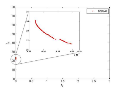
(a) NSGA-II

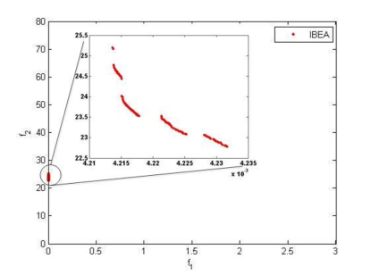
(b) IBEA

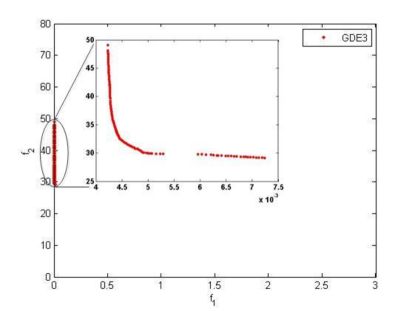
(c) GDE3

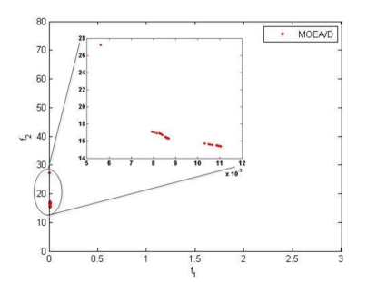
(d) MOEA/D

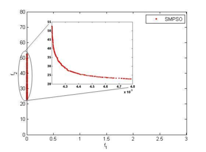
(e) SMPSO

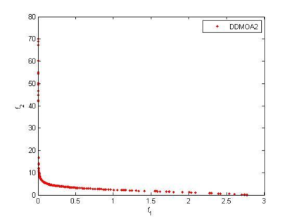
(f) DDMOA2

Figure 2. Trade-off curves obtained by six different algorithms.

Figure 2 depicts the sets containing all the nondominated solutions obtained by each algorithm after 30 runs. The total infected human population is shown in the x-axis ($f_{1}$). The total cost of insecticide is shown in the y-axis ($f_{2}$). One can easily observe that all EMO algorithms, with the exception of DDMOA2, face significant difficulties in obtaining a set of well-distributed nondominated solutions in the objective space. The obtained solutions are located in very small regions, while the majority of the search space remains unexplored (Figures 2(a)–2(e)). However, DDMOA2 is the only algorithm able to provide a good spread in the obtained nondominated solutions (Figure 2(f)). DDMOA2 extensively explores the search space and provides a wide range of trade-off solutions. Even the visual comparison of the obtained results allows to conclude that DDMOA2 performs significantly better on this problem compared to all the other tested algorithms.

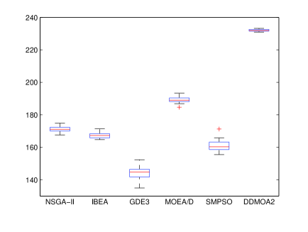
(a) distribution of hypervolume values

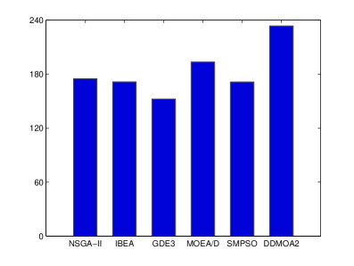
(b) total hypervolume

Figure 3. Performance comparison of the algorithms in terms of the hypervolume on the dengue transmission model.

To quantitatively assess the outcomes produced by the algorithms, the hypervolume [29] is calculated using $(f_{1},f_{2})=(3,80)$ as a reference point. Performance comparison of the algorithms with respect to the hypervolume is shown in Figure 3. The boxplots representing the distributions of the hypervolume values over the runs for each algorithm are depicted in Figure 3(a). It is interesting to note that the performance of genetic algorithms, namely NSGA-II (dominance-based) and IBEA (indicator-based), seems to be quite similar. However, NSGA-II gives a better spread of solutions that results in slightly higher values of the hypervolume. Two DE-based algorithms, namely GDE3 (dominance-based) and MOEA/D (scalarizing-based), perform differently. GDE3 has the worst performance, while MOEA/D behaves the best without considering DDMOA2. It can also be observed that the only PSO-based algorithm performs poorly. In turn, DDMOA2 yields the highest values of the hypervolume when compared to the other EMO algorithms. Moreover, the small variability of the achieved values highlights the robustness of DDMOA2. Performance comparison with respect to the total hypervolume achieved by all nondominated solutions obtained by each algorithm is presented in Figure 3(b). The data presented in this plot are consistent with the previous observations, being DDMOA2 again the algorithm with the best performance.

4.2. Problem Difficulties

To better understand the difficulties in solving this multiobjective optimization problem, $10^{5}$ points are sampled within the $1001$-dimensional unit hypercube (the feasible decision space) using a uniform distribution. Figure 4 illustrates the mapping of these points into the objective space. It can be observed that the uniform distribution of solutions in the decision space does not correspond to a uniform distribution in the objective space. Solutions are mapped into a relatively small region of the objective space. Thus, the probability of getting solutions in the region shown in Figure 4 is much higher than anywhere in the objective space. So there exists a pretty significant bias that can easily deceive the operators of evolutionary algorithms.

Another difficulty that significantly exacerbates the above discussed problem bias is related with the high dimensionality of the decision space. It is well known that the volume of the decision space increases exponentially with the number of decision variables. This means that in higher dimensions it is required to maintain much larger populations in order to have a similar coverage of the decision space as in the lower dimensions. This effect is called the curse of dimensionality [1].

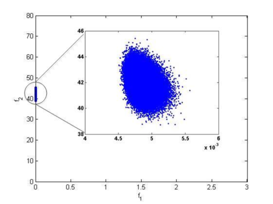
Figure 4. Mapping of uniformly sampled points in the decision space into the objective space defined by the dengue transmission model.

The discussed performance comparison of different algorithms reveals that all of the considered state-of-the-art EMO algorithms face significant difficulties dealing with such problem properties. Popular traditional evolutionary operators to perform the search in the decision space (including genetic algorithm-based, differential evolution-based and particle swarm optimization-based variation operators) perform poorly due to aforementioned difficulties. Moreover, most existing algorithms are typically tested on artificial benchmarks with up to 30 decision variables. As a result, they often become useless for large-scale problems that are highly common in real-world applications. On the other hand, DDMOA2 is a hybrid algorithm, which uses the concepts of traditional and stochastic optimization methods. Its local search procedure used to find descent directions explores extensively the decision space, working somewhat like global search in the case of this problem. It appears to be much more effective than pure evolutionary variation operators. Since DDMOA2 uses information about descent directions for different objectives to produce offspring, its variation operator is an intrinsically multiobjective one, contrary to the other algorithms. These features become extremely useful when solving this problem, showing the superiority of hybrid methodologies in algorithms’ design.

4.3. Dengue Dynamics

For this particular real-world problem, the above analysis allows to conclude that DDMOA2 works significantly better than the other considered algorithms. However, from a decision maker’s perspective, instead of comparing the performance of EMO algorithms, the main concern is a set of optimal solutions. Therefore, in the following we are focusing on presenting optimal solutions corresponding to the most effective ways of fighting the dengue epidemics.

To ensure the near optimality properties of obtained trade-off solutions, we perform local search using all the nondominated solutions returned by DDMOA2. For this purpose, we use the normal constraint (NC) method proposed by Messac and Mattson [17]. First, extreme solutions for all objectives are improved using a single-objective optimization algorithm. Then, the obtained solutions are used to construct the simplex with 300 uniformly distributed points. Finally, for each NC subproblem, from the obtained nondominated set we select a solution performing the best on the corresponding NC subproblem as the initial point to optimize this subproblem. As single-objective optimizer we use the MATLAB^® built-in function fmincon. Since not all solutions optimal for the NC subproblems may correspond to the Pareto optimal solutions, we discard all dominated solutions from the resulting set.

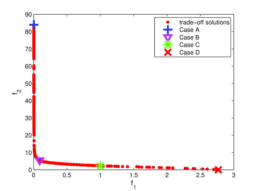
Figure 5. Trade-off curve for the infected population and control.

Figure 5 presents all the nondominated solutions obtained afterwards. It can be observed that the range of the trade-off curve has been extended compared to the results shown in Figure 2(f). Further observing this figure, one can see that for the insecticide cost in the range $0\leq f_{2}\leq 5$ there is almost a linear dependency between the infected human population ($f_{1}$) and the insecticide cost ($f_{2}$). Hence, reducing the number of infected humans from the worst scenario to $0.5$ can be done at a relatively low cost. However, starting from some further point, reducing the number of infected humans can be achieved through exponential increase in spendings for insecticide. Thus, even a small decrease in the number of infected humans corresponds to a high increase in expenses for insecticide. Scenarios represented by this part of the trade-off curve can be unacceptable from the economical point of view. Furthermore, it should be noted that even with the maximum spending it is not possible to eradicate the disease, being 0.0042 the lowest obtained value for the infected population.

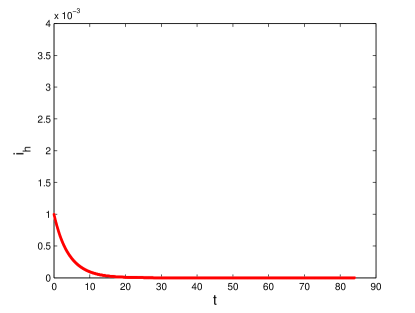
(a) Case A

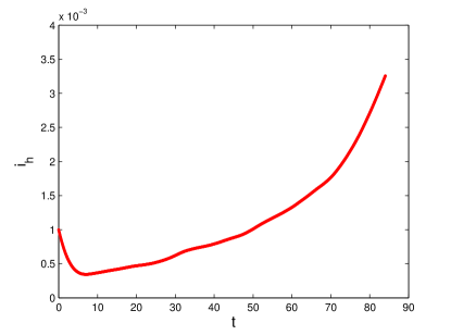
(b) Case B

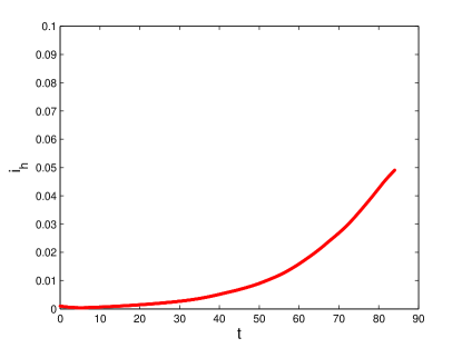
(c) Case C

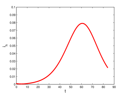
(d) Case D

Figure 6. Different scenarios of the dengue epidemic.

Additionally, Figure 5 presents four distinct points (Case A, Case B, Case C, and Case D) representing different parts of the trade-off curve, and, consequently, different scenarios of the dengue epidemic. For each case, Figure 6 plots the dynamics of the numbers of infected humans over the considered period of time.

Case A represents the medical perspective, when the number of infected humans is the lowest. From Figure 6(a), one can see that the number of infected people decreases from the very beginning. However, it is achieved through a huge expense for the insecticide.

Case B represents the region of the trade-off curve where an exponential dependency between the infected humans and the control begins. From Figure 6(b), it can be seen that, at the beginning, the number of infected humans decreases slightly. Thereafter, it grows steadily.

Case C represents the part of the trade-off curve with seemingly linear dependency between the two objectives. Figure 6(c) shows that in this case the number of infected humans grows from the very first moment. A more rapid grow is observed in the second half of the considered period of time.

Finally, Case D represents the economical perspective, when the treatment for infected population is neglected and the main concern is the saving from not performing insecticide campaigns. Figure 6(d) illustrates that in Case D the number of infected humans grows rapidly from the very beginning, reaching its peak approximately on the 60th day. After that the number of infected people decreases. This case corresponds to the worst scenario from the medical point of view.

4.4. Methods Comparison

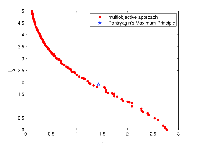
Figure 7. Solutions obtained using the multiobjective approach and Optimal Control Theory.

Finally, we compare the multiobjective approach discussed in this paper with the traditional technique based on the Optimal Control Theory commonly used to deal with such types of problems. Figure 7 shows the region of trade-off curve with $0\leq f_{2}\leq 5$ and a solution obtained using Pontryagin’s Maximum Principle. From this figure, it can be seen that there are solutions on the trade-off curve obtained using the multiobjective approach, which dominate the solution obtained using the Optimal Control Theory. Additionally, as it is shown in Figure 5 and can be seen in Figure 7, the multiobjective approach allows to find a number of other solutions that are incomparable with respect to the solution obtained using Pontryagin’s Maximum Principle. All these trade-off solutions provide more valuable information about the dengue epidemic, offering a variety of potential strategies to fight the disease. This highlights the advantages of a multiobjective approach compared to traditional techniques for finding the optimal control.

5. Conclusions

We proposed a multiobjective approach to find the optimal control to manage financial expenses caused by the outbreak of the dengue epidemic. We formulated the optimization problem with two objectives, including the system of differential equations modelling the disease. The first objective represents expenses due to the infected population. The second objective represents the cost of applying insecticide in order to fight the disease. We sought the optimal control simultaneously optimizing these clearly conflicting objectives. The obtained trade-off solutions reveal different perspectives on applying insecticide: a low number of infected humans can be achieved spending larger financial recourses, whereas low spendings for prevention campaigns result in significant portions of the population affected by the disease. At the same time, a number of other solutions represent different trade-offs between the objectives. Once the whole range of optimal solutions is obtained, the final decision on the control strategy can be made taking into consideration the available financial resources and goals of public health care. The analysis of different approaches to find the optimal control in the proposed model shows that the multiobjective approach presents clear advantages compared to the traditional approach based on the Optimal Control Theory. Additionally, the performance comparison of different multiobjective optimization algorithms is carried out on the optimization problem resulting from the proposed modelling approach. The obtained results show that the hybrid methodology significantly outperforms the traditional evolutionary algorithms. DDMOA2 appears to be the only among considered algorithms capable to find a wide range of trade-off solutions, whereas the other tested EMO algorithms face significant difficulties in solving this problem: the obtained solutions are located in small regions of the objective space. We believe that the promising results presented here will promote multiobjective modelling and will motivate further research in the design of hybrid and local search-based multiobjective optimization algorithms, which until now received relatively limited attention.

Acknowledgments

This work has been supported by the Portuguese Foundation for Science and Technology (FCT) in the scope of projects UID/CEC/00319/2013 (ALGORITMI R&D Center) and UID/MAT/04106/2013 (CIDMA).

References

- [1] R. Bellman. Dynamic Programming. Princeton Univ. Press, Princeton, NJ, 1957.
- [2] H.-G. Beyer and H.-P. Schwefel. Evolution strategies: A comprehensive introduction. Natural Computing, 1(1):3–52, 2002.
- [3] C. A. Coello Coello, G. B. Lamont, and D. A. Van Veldhuizen. Evolutionary Algorithms for Solving Multi-Objective Problems. Genetic and Evolutionary Computation, Springer, New York, 2007.
- [4] K. Deb. Multi-Objective Optimization using Evolutionary Algorithms. Wiley-Interscience Series in Systems and Optimization. John Wiley & Sons, 2001.
- [5] K. Deb, A. Pratap, S. Agarwal, and T. Meyarivan. A fast and elitist multiobjective genetic algorithm: NSGA-II. IEEE Transactions on Evolutionary Computation, 6(2):182–197, 2002.
- [6] R. Denysiuk, L. Costa, and I. Espírito Santo. DDMOA2: Improved descent directions-based multiobjective algorithm. In Proceedings of the Conference on Computational and Mathematical Methods in Science and Engineering, CMMSE’13, pages 513–524, 2013.
- [7] R. Denysiuk, L. Costa, and I. Espírito Santo. A new hybrid evolutionary multiobjective algorithm guided by descent directions. Journal of Mathematical Modelling and Algorithms in Operations Research, 12(3):233–251, 2013.
- [8] M. Derouich, A. Boutayeb, and E. Twizell. A model of dengue fever. Biomedical Engineering Online, 2(4):1–10, 2003.
- [9] G. J. Devine, E. Z. Perea, G. F. Killen, J. D. Stancil, S. J. Clark, and A. C. Morrison. Using adult mosquitoes to transfer insecticides to aedes aegypti larval habitats. In Proceeding of the National Academy of Sciences of the United States of America, 2009.
- [10] J. J. Durillo and A. J. Nebro. jMetal: A Java framework for multi-objective optimization. Advances in Engineering Software, 42(10):760–771, 2011.
- [11] Y. C. Ho and D. L. Pepyne. Simple explanation of the no-free-lunch theorem and its implications. Journal of Optimization Theory and Applications, 115(3):549–570, 2002.
- [12] E. J. Hughes. MSOPS-II: A general-purpose many-objective optimiser. In Proceedings of the IEEE Congress on Evolutionary Computation, CEC’07, pages 3944–3951, 2007.
- [13] H. Ishibuchi, T. Doi, and Y. Nojima. Incorporation of scalarizing fitness functions into evolutionary multiobjective optimization algorithms. In Proceedings of the Conference on Parallel Problem Solving from Nature, PPSN’06, pages 493–502, 2006.
- [14] S. Kukkonen and J. Lampinen. GDE3: the third evolution step of generalized differential evolution. In Proc. IEEE Congress on Evolutionary Computation, CEC’05, 443–450, 2005.
- [15] H. Li and Q. Zhang. Multiobjective optimization problems with complicated Pareto sets, MOEA/D and NSGA-II. IEEE Trans. Evolutionary Computation, 13(2):284–302, 2009.
- [16] W. L. Loh. On latin hypercube sampling. Annals of Statistics, 33(6):2058–2080, 1996.
- [17] A. Messac and C. Mattson. Normal constraint method with guarantee of even representation of complete Pareto frontier. AIAA Journal, 42:2101–2111, 2004.
- [18] Ministério da Saúde de Cabo Verde. Dengue. http://www.minsaude.gov.cv, January 2012.
- [19] A. J. Nebro, J. J. Durillo, J. García-Nieto, C. A. Coello Coello, F. Luna, and E. Alba. SMPSO: A new PSO-based metaheuristic for multi-objective optimization. In Proceedings of the Symposium on Computational Intelligence in Multicriteria Decision-Making, MCDM’09, pages 66–73, 2009.
- [20] M. Otero, N. Schweigmann, and H. G. Solari. A stochastic spatial dynamical model for aedes aegypti. Bulletin of Mathematical Biology, 70(5):1297–1325, 2008.
- [21] L. S. Pontryagin, V. G. Boltyanskii, R. V. Gamkrelidze, and E. F. Mishchenko. The mathematical theory of optimal processes. International series of monographs in pure and applied mathematics. Pergamon Press, New York, USA, 1964.
- [22] H. S. Rodrigues, M. T. T. Monteiro, and D. F. M. Torres. Bioeconomic perspectives to an optimal control dengue model. Int. J. Comput. Math., 90(10):2126–2136, 2013. arXiv:1303.6904
- [23] H. S. Rodrigues, M. T. T. Monteiro, and D. F. M. Torres. Dengue in Cape Verde: vector control and vaccination. Math. Popul. Stud., 20(4):208–223, 2013. arXiv:1204.0544
- [24] H. S. Rodrigues, M. T. T. Monteiro, D. F. M. Torres, and A. Zinober. Dengue disease, basic reproduction number and control. Int. J. Comput. Math., 89(3):334–346, 2012.
- [25] V. Torczon. On the convergence of pattern search algorithms. SIAM J. Optim., 7:1–25, 1997.
- [26] D. H. Wolpert and W. G. Macready. No free lunch theorems for optimization. IEEE Transactions on Evolutionary Computation, 1(1):67–82, 1997.
- [27] A. Zhou, B.-Y. Qu, H. Li, S.-Z. Zhao, P. N. Suganthan, and Q. Zhang. Multiobjective evolutionary algorithms: A survey of the state of the art. Swarm and Evolutionary Computation, 1(1):32–49, 2011.
- [28] E. Zitzler and S. Künzli. Indicator-based selection in multiobjective search. In Proceedings of the Conference on Parallel Problem Solving from Nature, PPSN’04, pages 832–842, 2004.
- [29] E. Zitzler and L. Thiele. Multiobjective optimization using evolutionary algorithms – A comparative case study. In Proceedings of the Conference on Parallel Problem Solving From Nature, PPSN’98, pages 292–304, 1998.