Velocity resolved [C ii] spectroscopy of the center and the BCLMP 302 region of M 33 (HerM 33es)

Abstract

Context. The forbidden fine structure transition of C⁺ at 158 $\mu$m is one of the major cooling lines of the interstellar medium (ISM).

Aims. We aim to understand the contribution of the ionized, atomic and molecular phases of the ISM to the [C ii] emission from clouds near the dynamical center and the BCLMP302 H ii region in the north of the nearby galaxy M 33 at a spatial resolution of 50 pc.

Methods. We combine high resolution [C ii] spectra taken with the HIFI spectrometer onboard the Herschel satellite with [C ii] Herschel-PACS maps and ground-based observations of CO(2-1) and H i. All data are at a common spatial resolution of 50 pc. Correlation coefficients between the integrated intensities of [C ii], CO(2–1) and H i are estimated from the velocity-integrated PACS data and from the HIFI data. We decomposed the [C ii] spectra in terms of contribution from molecular and atomic gas detected in CO(2–1) and H i, respectively. At a few positions, we estimated the contribution of ionized gas to [C ii] from the emission measure observed at radio wavelengths.

Results. In both regions, the center and BCLMP302, the correlation seen in the [C ii], CO(2–1) and H i intensities from structures of all sizes is significantly higher than the highest correlation in intensity obtained when comparing only structures of the same size. The correlations between the intensities of tracers corresponding to the same velocity range as [C ii], differ from the correlation derived from PACS data. Typically, the [C ii] lines have widths intermediate between the narrower CO(2–1) and broader H i line profiles. A comparison of the spectra shows that the relative contribution of molecular and atomic gas traced by CO(2–1) and H i varies substantially between positions and depends mostly on the local physical conditions and geometry. At the positions of the H ii regions, the ionized gas contributes between 10–25% of the observed [C ii] intensity. We estimate that 11–60% and 5–34% of the [C ii] intensities in the center and in BCLMP302, respectively, arise at velocities showing no CO(2–1) or H i emission and could arise in CO-dark molecular gas. The deduced strong variation in the [C ii] emission not associated with CO and H i cannot be explained in terms of differences in $A_{\rm V}$, far-ultraviolet radiation field, and metallicity between the two studied regions.

Conclusions. The relative amounts of diffuse (CO-dark) and dense molecular gas possibly vary on spatial scales smaller than 50 pc. In both regions, a larger fraction of the molecular gas is traced by [C ii] than by the canonical tracer CO. Correlations between observed intensities of [C ii], CO, and H i crucially depend on the spatial and spectral resolution of the data and need to be used carefully, in particular, for extragalactic studies. These results emphasize the need for velocity-resolved observations to discern the contribution of different components of the ISM to [C ii] emission.

1 Introduction

Under a wide range of astrophysical conditions, including ionized, atomic, and molecular phases of the interstellar medium (ISM), a significant fraction of gaseous carbon is in the form of C⁺. The forbidden fine structure transition ³P_3/2$\rightarrow$³P_1/2 of C⁺ (with $\Delta$E=91 K), written as [C ii], is easily excited and is typically optically thin and not affected by extinction in most astrophysical environments. Thus, [C ii] is not only an excellent coolant of the neutral gas exposed to the ionizing flux of nearby early-type stars, but also an excellent probe of stellar radiation fields and their effects on the physical conditions of the ambient neutral gas.

Early studies of [C ii] emission from nearby galaxies revealed that the line contributes 0.1% to 1% of the total far-infrared (FIR) continuum and is strongly correlated with the strength of the CO(1–0) rotational line (Crawford et al. 1985; Stacey et al. 1991; Madden et al. 1993; Malhotra et al. 2001). These studies suggested that [C ii] line emission on galactic scales mostly originates from the warm, dense photodissociated surfaces of clumps in molecular clouds, known as photodissociation regions (PDRs). The PDRs are created by far-UV (FUV; 6 eV$<$h$\nu<$13.6 eV) photons from nearby OB stars or the general interstellar radiation field (ISRF). Moderate density ($n_{\rm H}<10^{4}$ cm^-3) and temperature (30 – 100 K) clouds in the PDRs are primarily cooled by the 158 $\mu$m [C ii]  line, with [O i] at 63 $\mu$m being responsible for the cooling at high FUV fields and large gas densities. However, high spatial resolution ($<$300 pc) observations of nearby galaxies that resolve individual giant molecular clouds (GMCs) show the correlation between [C ii] and CO(1–0) to be much weaker (Rodriguez-Fernandez et al. 2006; Mookerjea et al. 2011; Kramer et al. 2013). The question of disentangling the contributions of the components (PDR, cold neutral medium (CNM), and ionized gas) to the [C ii] emission from galaxies can only be appropriately addressed via observations of several emission lines at high spatial and spectral resolution.

In the absence of multiple transitions of C⁺, comparison of spectral profiles with those of CO, H i and other tracers at resolutions comparable to ground-based single dish telescopes are crucial and the velocity-resolved high spatial resolution capabilities of the recent far-infrared missions HIFI/Herschel and GREAT/Stratospheric Observatory for Far Infrared Astronomy (SOFIA) have made these possible. Located at a distance of 840 kpc (Freedman et al. 1991), the Triangulum galaxy M 33 is a nearby, gas-rich disk galaxy with half the solar metallicity, which allows for this type of a coherent survey at high spatial and spectral resolution. As part of the Herschel Key Program HerM 33es (Kramer et al. 2010), selected regions along the major axis of M 33 were mapped with PACS in [C ii], [O i] (63 $\mu$m) and [N ii] (122 $\mu$m) (Mookerjea et al. 2011, ;Nikola et al. (in prep)). These PACS regions are further probed along selected cuts with velocity-resolved spectra of [C ii] at 158 $\mu$m using HIFI (Braine et al. 2012). Higdon et al. (2003) performed a detailed study of the nucleus of M 33 and six selected H ii regions using seven FIR fine-structure lines observed with ISO/LWS. The present Herschel observations also follow up on the ISO/LWS observations of [C ii] integrated intensities at 280 pc resolution along the major axis of M 33 (Kramer et al. 2013), encompassing the regions observed in [C ii] with Herschel. In this paper, we present higher resolution [C ii] lines observed with HIFI in the central region of M 33 and the H ii region BCLMP302 along two 140″ long strips approximately oriented along the north-south and east-west direction in each of the two regions. The BCLMP302 region is located at a galactocentric distance of 2 kpc in the northern spiral arm. The HIFI spectra sample multiple emission features detected in CO and dust continuum emission, with sizes typically corresponding to GMCs. The HIFI [C ii] data are compared with CO(2–1) and H i spectra tracing the molecular and atomic components of the neutral interstellar medium (Gratier et al. 2010). The primary aim of the paper is to utilize the velocity information in the newly observed HIFI [C ii] data to identify the phase of the ISM that mainly contributes to the [C ii] emission and also to derive its physical properties. The work presented here extends the [C ii] PACS and HIFI (single-position) observations of BCLMP 302 (Mookerjea et al. 2011). It also compares the properties of the [C ii] emitting regions in the central region of M 33 and BCLMP302 with the H ii region BCLMP691, located approximately at a galactocentric distance of 3.5 kpc (Braine et al. 2012).

2 Observations

2.1 Herschel: [C ii] with HIFI

We have observed the ³P_3/2–³P_1/2 transition of C⁺ at 1900536.9 MHz with the Heterodyne Instrument for Far Infrared astronomy (HIFI) onboard Herschel (Pilbratt et al. 2010; de Graauw et al. 2010). The observations consisted of two load-chopped, on-the-fly (OTF) scans each of $\sim 140$″ length with position angle (PA) of 22.5^∘ and 112.5^∘ for an area around the center of M 33 and with PA of 45^∘ and 135^∘ for a region around the H ii region BCLMP302 in M 33. The measurements presented here correspond to the Herschel observation identification (Obsids) 1342213340 (OD623), 1342213702 (OD630), 1342213741 (OD632) and 1342214315 (OD642). The observations were performed on 26 January, 2, 4, and 14 February, 2011. The offsets for the OTF positions in the central region are given relative to the position $\alpha_{2000}$ = 01^h33^m48$\aas@@fstack{s}$20 $\delta_{2000}$ = 30^∘39′21$\aas@@fstack{\prime\prime}$4 with the east-west (EW) cut passing through the dynamical center of M 33. For the BCLMP302 region, the corresponding offsets are given relative to $\alpha_{2000}$ = 01^h34^m06$\aas@@fstack{s}$30 $\delta_{2000}$ = 30^∘47′25$\aas@@fstack{\prime\prime}$3. At the frequency of [C ii], the Herschel/HIFI beam size is 11$\aas@@fstack{\prime\prime}$1, the forward efficiency $F_{\rm eff}$ is 96%, and the main beam efficiency $B_{\rm eff}$ is 59% (Mueller et al. 2014).

The HIFI Wide Band Spectrometer (WBS) was used with spectral resolution of 1.1  MHz (0.17 km s^-1) over an instantaneous bandwidth of 2.4 GHz at 1.9 THz. The [C ii] spectra were smoothed to a resolution of 1.2 km s^-1 to improve the signal-to-noise ratios per channel.

Data was reduced using the standard HIFI pipeline up to level 2 including HifiFitFringe, with the ESA supported-package HIPE 10.0 (Ott 2010). About 30% of the observed [C ii] spectra were found to suffer from the standing wave pattern seen in receivers with hot electron bolometers (HEB), which were corrected to a large extent via a tool employing the current matching technique provided by the Herschel helpdesk. The data were then exported as FITS files into CLASS/GILDAS format for subsequent reduction. The spectra on the two fully-sampled cuts for each region were averaged over 15″ and gridded into a 10″ grid (Fig. 2). We obtained the main beam brightness temperature, $T_{\rm mb}$, by multiplying the antenna temperature, $T_{\rm A}^{\ast}$, by $F_{\rm eff}$/$B_{\rm eff}$.

The gridded spectra from the central region of M 33, which we selected for further analysis, have typical integration times between 20 to 40 minutes and show an rms of 48 to 62 mK for a velocity resolution of 1.2 km s^-1. Similarly, for BCLMP302 at a velocity resolution of 1.2 km s^-1 the final rms noise varies between 42 to 54 mK with most positions having an integration time of 54 mins. The rms levels mentioned above are in the $T_{\rm mb}$ scale.

2.2 Complementary data

The PACS/Herschel spectroscopy observations of [C ii], [OI] 63 $\mu$m, and [N ii] 122 $\mu$m contain 22 (including BCLMP302 and the center) independent observations of smaller regions, each covered by a 3x3 raster with the PACS array, and combined they result in a strip map along the major axis of M33. In total, these observations cover a region of about 45′ $\times$ 2$\aas@@fstack{\prime}$5 at a resolution of 12″ with some gaps in the northern part. The complete PACS spectroscopic dataset will be presented in Nikola et al. (in prep). The H i VLA and CO(2–1) HERA/30m spectra at the HIFI [C ii] positions were extracted from the maps presented by Gratier et al. (2010). The original angular resolutions of the H i and CO(2–1) data were 5″ and 12″, respectively. The spectral resolutions of the H i and CO(2–1) data were 2.6 km s^-1 and 1.3 km s^-1, respectively. We also use the Spitzer MIPS 24 $\mu$m data presented by Tabatabaei et al. (2007), and the HerM 33es PACS and SPIRE maps at 100, 160, 250, 350 and 500 $\mu$m (Verley et al. 2010; Boquien et al. 2010; Kramer et al. 2010; Boquien et al. 2011; Xilouris et al. 2012). All complementary Herschel data up to 160 $\mu$m were smoothed to a resolution of 12″ for direct comparison with [C ii].

3 Global morphology of [C ii] emission in M 33

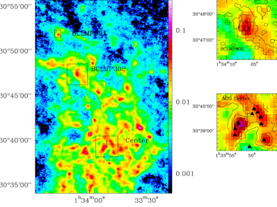
Figure 1: PACS 160 $\mu$m continuum image of M 33 (Kramer et al. 2010). The boxes corresponding to the regions around the H ii regions BCLMP302, BCLMP691 and the center of M 33 are indicated. The cross shows the position of the dynamical center of M 33. Zoomed in images of the two regions studied, the center and BCLMP302, are shown to the right, with contours indicating the integrated [C ii] intensities observed with PACS (Mookerjea et al. (2011); Nikola et al. in prep). The known H ii regions in the central region (Gordon et al. 1999) are shown as filled triangles.

Figure 1 shows the 160 $\mu$m PACS continuum map of M 33 with squares indicating the central, BCLMP302, and BCLMP691 regions. Contours of [C ii] intensity maps observed with PACS for the two regions presented here (central and BCLMP302) are overlayed on the 160 $\mu$m continuum map and are shown in the insets of Fig. 1. For both regions, the [C ii] integrated intensity contours follow the dust continuum distribution rather closely. Toward the center and in BCLMP302 region the [C ii] intensity maps are also morphologically similar to the tracers of star formation such as the H$\alpha$ emission. The ISO/LWS [C ii] study along the major axis also shows a relatively constant correlation with the H$\alpha$ and the far-infrared continuum; the $I_{\rm CII}$/$I_{\rm FIR}$ ratio stays constant at 0.8% in the inner 4.5 kpc of M 33, rising in the outskirts to values of 3% at 6 kpc radial distance (Kramer et al. 2013).

Figure 2 shows the observed [C ii] spectra at 29 positions on a 10″ grid along the two cuts observed in each of the two regions in the center of M 33 and around BCLMP302, overlayed on the MIPS 24 $\mu$m image. Out of the 29 observed positions in each of the regions, [C ii] emission has been detected at 23 and 19 positions in the central and BCLMP302 regions, respectively.

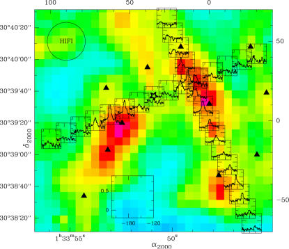
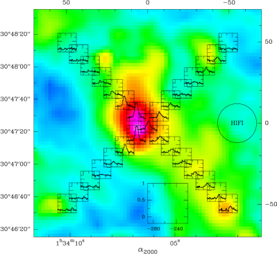
Figure 2: MIPS 24 $\mu$m image of the regions around the center of M 33 (left) and the H ii region BCLMP302 (right) in M 33 overplotted with the observed spectra of [C ii]. Filled black triangles in the left box denote positions of the GMCs identified by Gratier et al. (2012) and the star indicated on the eastern part of the E-W cut shows the position of the dynamical center of M 33. The HIFI beam at 1.9 THz is also shown as inset. All spectra are shown on a 10″ grid. Empty boxes show the intensity and velocity scales for the spectra plotted.

3.1 M 33 central region

The dynamical center ($\alpha_{2000}$=01^h33^m50$\aas@@fstack{s}$9 $\delta_{2000}$=30^∘39′35.8″; Jarrett et al. 2003) of M 33 is unspectacular in both [C ii] and dust continuum, with no emission feature located exactly at that position. However, two intersecting ridges, consisting of bright infrared peaks, are discernible and the HIFI cuts are approximately oriented along the two ridges. Within the observed region at the center of M 33, 12 GMCs (# 95, 99, 100, 107, 108, 109, 110, 111, 114, 116, 175, and 176; Gratier et al. 2012) and ten H ii regions (Gordon et al. 1999) are already identified (Figs. 1,2).

The cuts along which the [C ii] HIFI observations are performed, extend approximately along the north-south (N-S) and the east-west (E-W) directions (Fig. 2). The N-S cut passes through several bright continuum sources, while the E-W cut traces the outskirts of a few of the continuum sources. Because of the position of the cuts across the dynamical center of M 33, the v_LSR of peak [C ii] emission also changes by up to 40 km s^-1 along the two cuts (Sec. 4). The E-W cut passes through the dynamical center of M 33 and we do not detect any [C ii] emission at the center with HIFI. The [C ii] intensity measured by PACS at the center of M 33 is 5.9 K km s^-1, which for the typical velocity spread of 50 km s^-1 of the [C ii] line in this region corresponds to a peak $T_{\rm mb}$ of 110 mK. The rms measured in the HIFI spectrum at the position of the center at a resolution of 1.2 km s^-1 is 71 mK. Thus the non detection of [C ii] emission at the center in the HIFI data is consistent with the PACS observations. Depending on the position of the HIFI [C ii] beam relative to the location of molecular clouds, the [C ii] spectra exhibit one or more velocity components. In addition, the [C ii] intensities decrease with increasing distance from the dust continuum peaks.

3.2 BCLMP302

The mid- and far-infrared dust continuum emission from the BCLMP302 region is dominated by the H ii region itself and extends along the NE-SW direction with a secondary peak approximately 75″ to the SW of the main peak (Fig. 2). Previous PACS observations have shown that the [C ii] intensities in this region correlate well with the dust continuum and H$\alpha$ emission, thus broadly tracing star- forming regions (Mookerjea et al. 2011). However, the [C ii] and [O i] 63 $\mu$m intensities do not correlate well with either the CO(2-1) or the H i emission. One of the two HIFI cuts is aligned with the dust continuum emission ridge extending in the NE-SW direction and passes through the secondary peak to the SW. We detected [C ii] emission primarily close to the dust continuum peaks, although we see no intensity enhancement toward the SW peak. The spectra typically show a single velocity component except at a few positions immediately to the SW of the main dust continuum peak, where an additional narrow velocity component is also detected.

4 Integrated [C ii] intensities

4.1 Spatial distribution

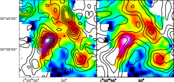
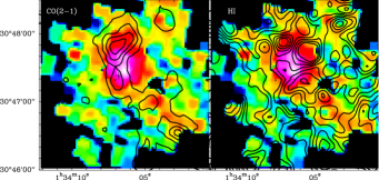
Figure 3: Overlay of CO(2–1) ($left$) & H i ($right$) contours on the PACS intensity map of [C ii] for the central ($top$) and BCLMP302 ($bottom$; Mookerjea et al. (2011)) regions. The [C ii] data has no velocity information and CO(2–1) and H i spectra have been integrated over the entire range of velocities. The white and black regions in the top and bottom panels respectively, indicate regions not mapped with PACS.

Figure 3 shows a comparison of the maps of integrated intensities of [C ii] (observed with PACS), CO(2–1), and H i for the central region (top panel) of M 33 and BCLMP302 (bottom panel). Correspondence between the emission from the three tracers is typically considered to be an indicator of the physical proximity or association of the emitting atomic, molecular, and PDR gas. In the central region, the main emission features of [C ii] agree in position with CO(2–1) and H i, and also with tracers of star formation such as the 160 and 24 $\mu$m dust continuum or H$\alpha$.

Mookerjea et al. (2011) used the PACS [C ii] data to perform an analysis of the linear correlation of the integrated intensities of CO(2–1) and H i relative to those of [C ii] for the BCLMP302 region. These authors derived linear correlation coefficients of 41% and 22% for [C ii]–CO and [C ii]–H i, respectively, using the same maps as in Fig. 3. We perform a similar analysis of the [C ii] PACS data for the mapped region around the center of M 33 and find the global correlation coefficients to be 71% and 69% for the [C ii]–CO(2–1) and [C ii]–H i integrated intensities, respectively.

The correlation coefficients presented above measure the correspondence between the structures in the maps, independent of their size, averaged over the entire map. For a scale-dependent investigation that only compares structures with a particular size, we measure the correspondence on a scale-by-scale basis. For this analysis, we use the wavelet-based weighted cross-correlation (WWCC) tool developed by Arshakian & Ossenkopf (2015) to study the degree of correlation of structures seen in a pair of maps as a function of their spatial scale. The method first filters the maps to be compared with a wavelet of a characteristic size so that only structures of that size remain in the maps, and in a second step computes the correlation between the filtered maps. With this approach, only structures of the same scale are compared. Use of different wavelet sizes results in a spectrum of correlation coefficients. In case of systematic shifts of characteristic structures between the maps, the tool can also measure their mutual displacement. Figure 4 shows the correlation coefficient as a function of scale for the [C ii]–CO(2–1) and [C ii]–H i maps for both the central and the BCLMP302 regions.

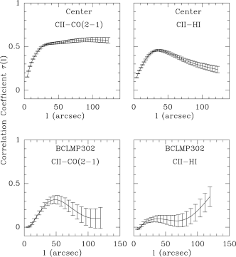
Figure 4: Correlation coefficient as a function of scale for the integrated intensity maps presented in Fig. 3.

In the center of M 33, we find an increasing correlation both between [C ii] and CO(2–1) and between [C ii] and H i at scales up to about 30″ (Fig. 4). As seen in the maps, individual smaller structures are typically displaced between the different maps, but the main emission peaks, having a size of about 30″, agree in their rough location. When considering larger scale structures, the relative contribution of those peaks matters as they merge. In H i the strongest emission is located in the western peak and the overall emission is very extended while the [C ii] and CO(2–1) emission is highly concentrated at the eastern peak. This leads to constant and high correlation between [C ii] and CO(2–1) at large scales and a corresponding decreasing correlation with H i.

In BCLMP302, we even find a small anticorrelation between the species at the smallest scales. The maps already show that the location of the peaks is rather disjunct. When comparing [C ii] and CO(2–1), the correlation increases again up to scales of about 45″, the size of the main emission feature seen in both species. The correlation coefficient, however, is less than 30% as the internal structure of both peaks is very different and there is also a systematic offset. When looking at larger scales, the correlation drops here because the two CO(2–1) emission features in the north start to merge so that the main structure is shifted to the north relative to the centrally peaked main emission seen in [C ii]. When comparing [C ii] with H i, the situation is different. The coefficient is less than 10% for all structures that can be identified by eye in Fig. 3, but at the largest scales the individual clumps in the overall extended H i emission start to merge into a centrally peaked structure that appears more similar to the centrally peaked [C ii] map.

Overall, we find that for both regions, the global correlation coefficients between [C ii], CO(2–1) and H i maps, derived considering structures of all sizes, are larger than even the peak of the correlation coefficient seen on a scale-by-scale basis. We also see that a good correlation measured at large scales is not at all necessarily related to a good correlation at smaller scales. Thus, observations with insufficient spatial resolution can easily be misleading. The possible implications of these results are discussed in Sect. 10.3.

4.2 Correlation plots

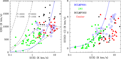
Figure 5: Correlation of integrated intensities of H i (left) and CO(2–1) (right) with [C ii] integrated intensities for BCLMP302 (black squares), central region (red triangles), and BCLMP691 (blue empty squares; Braine et al. 2012) and for positions along the major axis of M 33 measured with ISO/LWS at 280 pc resolution (green filled circles; Kramer et al. 2013). For the central and BCLMP302 region, [C ii], CO(2–1) and H i are integrated only over the range of velocities in which [C ii] is detected at the individual positions. The dashed curved lines in the left panel show the predicted $I$([C ii]) for low-density diffuse atomic H i clouds as a function of $I$(H i), corresponding to the pressures $P$ = 2000 and 8000 K cm^-3 for a kinetic temperature of 100 K. The box in dashed lines shows the region occupied by the [C ii] emitting H i clouds analyzed by the GOT C⁺ project (Langer et al. 2014). Both panels show lines (blue continuous) of proportionality to guide the eye.

The velocity-resolved [C ii] spectra observed with HIFI provide us with the unique opportunity of identifying the velocity range over which [C ii] is emitted. Consequently, it is possible to compare the intensities of CO(2–1) and H i integrated over the same velocity range where [C ii] is detected. Figure 5 shows a comparison of the H i and CO(2–1) intensities as a function of the [C ii] intensities at all positions observed with HIFI in the center and the BCLMP302 regions. All the integrated intensities were calculated over the velocity range ($\upsilon_{\rm min}$ to $\upsilon_{\rm max}$ in Tables 2 and 3) in which [C ii] emission is detected. For comparison, we have overplotted the [C ii], CO, and H i intensities measured with HIFI in the BCLMP691 region (Braine et al. 2012), as well as the results of the analysis of the ISO-LWS data taken along the major axis of M 33 (Kramer et al. 2013). Figure 5 also shows the region (dashed parallelogram) in the [C ii]–H i correlation graph occupied by the clouds detected in the Milky Way by the GOT C⁺ survey performed with Herschel/HIFI (Langer et al. 2014).

The [C ii] intensities measured by the ISO-LWS typically have values lower than those measured using HIFI, possibly because of the significantly larger size of the ISO beam (70″). The points belonging to the central and the BCLMP302 regions occupy separate areas in the [C ii]-H i correlation plot. For the same values of [C ii] intensities, the BCLMP302 positions show higher $I$(H i) as compared to the positions in the central region. This kind of a segregation is not seen in the [C ii]-CO(2–1) plot where the points from the two regions overlap significantly with each other. The points corresponding to BCLMP691 occupy essentially the same region in the [C ii]–H i correlation plot as the M 33 center, although the H i intensity from BCLMP691 remains almost constant. For the same values of $I$([C ii]), $I$(CO(2–1)) tends to be higher in BCLMP691 than in the other regions. The Galactic clouds detected by the GOT C⁺ survey typically have similar $I$([C ii]) as the M 33 clouds but somewhat lower $I$(H i). Comparison of M 33 and Galactic molecular clouds is strongly affected by the different spatial scales probed by the HIFI observations. Furthermore, for the Galactic observations within GOT C⁺ the beam size of H i observations was larger than the [C ii] beam.

Table 1 presents the linear correlation coefficients for the [C ii]–H i and the [C ii]–CO(2–1) scatterplots (Fig. 5) for the different datasets. We find that for the BCLMP302, BCLMP691, and ISO-LWS data along the major axis of M 33, the [C ii] intensities have a correlation coefficient $>65$% with CO(2–1), whereas in the center the correlation is somewhat poor. The correlation between [C ii]–H i also varies from region to region, with H i in BCLMP691 practically showing no correlation with [C ii]. For both the central and BCLMP302 region, the correlation coefficient for [C ii]–CO(2–1) and [C ii]–H i derived with the line velocity information appears to contradict the correlation coefficient estimated from the PACS observations of those region (Sec. 4.1).

Table 1: Linear correlation coefficients for the scatter plots in Fig. 5. Here $I$(CO(2–1) and $I$(H i) were estimated by integrating only over the velocity range over which [C ii] is detected.

Region	[C ii]–CO(2–1)	[C ii]–H i
Center	0.33	0.50
BCLMP302	0.67	0.61
BCLMP691	0.70	0.07
Major Axis	0.77	0.44
All	0.75	0.66

Thus, for the integrated intensities derived over selected velocity ranges (as for the center, the BCLMP302, and BCLMP691 regions) the [C ii]-CO(2–1) correlation varies drastically with location, with M 33’s outer arm regions showing higher correlations. The correlation between [C ii] and H i is generally worse than the [C ii]–CO(2–1) correlation, and also varies greatly between the different regions.

5 Results: position-velocity diagrams

5.1 Central region of M 33

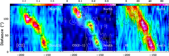
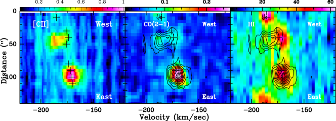
Figure 6: Position-velocity diagrams for [C ii], CO(2–1) and H i along the north-south (top) and east-west (bottom) directions in the central region of M 33. The contours in the middle and right panels correspond to [C ii] emission and range from 10% to 100% of the peak values of 0.6 and 0.8 K in steps of 10% for the NS and EW cuts, respectively. The color bar on top of each panel shows the color scale of the corresponding image in units of K. The crosses in all panels denote the nominal velocities due to galactic rotation obtained from H i spectra (see text).

Figure 6 shows the position-velocity (PV) diagrams along cuts oriented in the NS and EW directions for [C ii], CO(2–1) and H i of the region close to the center of M 33. For all three tracers, the velocity gradients observed toward the center of M 33 are dominated by the rotation of the galaxy. We first estimate the differences in velocities observed in the three tracers beyond the effect of rotation of the galaxy. For this, we have derived the velocity due to the galactic rotation by fitting a single-component Gaussian to H i spectra smoothed to a resolution of 10 km s^-1 at individual positions on the cut. The fitted H i velocities are indicated with crosses in Fig. 6. The velocities estimated from the H i spectra along both directions are consistent with the galactic rotation curve derived by Corbelli & Walterbos (cf. 2007) using H$\alpha$ data. The velocity due to rotation leads to gradients of 40 km s^-1 and 25 km s^-1 over a length of 140″ in the NS and EW directions, respectively.

For the NS cut, we find that the velocities of the peak emission of both [C ii] and CO(2–1) agree reasonably well with the centroid velocity of the H i emission up to a length of 70″ starting from the south (Fig. 6, top). Further north along the NS cut, (i) the CO(2–1) peak is shifted toward more northern positions relative to [C ii], and (ii) H i emission shows double emission peaks around 100″, of which the lower velocity peak is followed by [C ii] and CO(2–1). Along the EW direction, H i shows four emission peaks, out of which only one around 100″ from west matches the [C ii] and CO(2–1) peaks. The [C ii] emission peak at 50″ from west occurs at 16 km s^-1 lower velocity compared to H i, while CO(2–1), though not bright at this position, is closer in velocity to [C ii]. The redward shift in H i velocity relative to the velocities of [C ii] and CO(2–1) in the central region of M 33 could be indicative of local dynamics, which leads to differential motion between the diffuse atomic and molecular (or PDR) phases of the ISM. This also implies that toward the center of the galaxy the [C ii] emitting gas is better associated with the CO emitting PDRs than the H i emitting more diffuse atomic gas.

5.2 BCLMP302 region

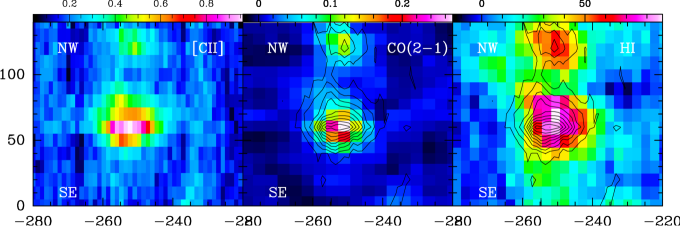
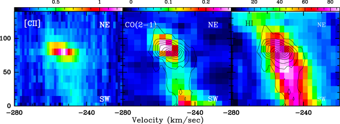
Figure 7: Position-velocity diagrams for [C ii], CO(2–1) and H i along the SE-NW (top) and SW-NE (bottom) directions for BCLMP302. The contours in the middle and right panels correspond to [C ii] emission and range from 20% to 100% of the peak value of 1.1 K and 0.8 K in steps of 10% for SE-NW and SW-NE cuts, respectively. The color bar on top of each panel shows the color scale of the corresponding image in units of K.

Similar to the central region, the [C ii] spectra in the two cuts along the SE-NW and SW-NE directions crossing BCLMP302 show broader line widths than the CO(2-1) lines, while the H i emission is only slightly broader than the [C ii] line (Fig. 7). Along the SE-NW cut all three tracers match well both velocity-wise and spatially. Along the SW-NE cut in the BCLMP302 region: (i) the velocities of the [C ii] and H i emitting clouds appear to match each other, while the CO(2–1) emission shows a redward shift by 10 km s^-1, and (ii) although the [C ii] and CO(2–1) emission peaks match spatially, the H i emission peak is shifted by 10–20″ to the SW.

While there is an overall similarity of the [C ii], CO(2–1) and H i position-velocity diagrams, both in the center and BCLMP302, in some locations strong [C ii] is detected at velocities significantly shifted relative to both the CO(2–1) and H i emission.

6 Excess [C ii] emission seen in the spectra

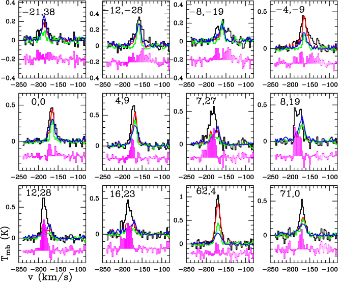
Figure 8: [C ii] (black), CO(2–1) (green), and H i (blue) spectra at selected positions in the center of M 33. The H i spectrum has been scaled by a factor of 0.005 for easier comparison. The fit to the observed [C ii] spectrum, as obtained from the method described in text, is shown in red and the residual spectrum (vertically offset) is shown in magenta.

Figures 8 and 9 show the [C ii], CO(2–1) and H i spectra at selected positions in the central and BCLMP302 regions of M 33. The positions in both regions were chosen based on the S/N ratio of the [C ii] spectra. In the central region, the [C ii] spectra show widths intermediate between the linewidths of H i and CO(2–1). Given the higher propensity of CO(2–1) to become optically thick it is understandable if both [C ii] and H i emission trace larger column densities of gas (Henkel & Wiklind 1997). As seen in the PV diagrams, at multiple positions the [C ii] spectra show additional features at velocities where very little or no CO(2–1) and/or H i emission are detected.

Ignoring the contribution of the ionized gas, the [C ii] emission may arise from (a) HI, (b) CO-traced H₂, (c) H/H₂ not traced by either H i or CO emission. In order to estimate the fraction of [C ii] emission arising from the component not detected in CO or H i, we fit the observed [C ii] spectrum at each position as a linear combination of the CO(2–1) and H i intensities. The fitting procedure does not make any assumption about the physical heating model (PDR, GMC, shocked ISM, XDR, CR). It maximizes the emission that could be associated with (a) and (b), and so determines the minimum profile associated with (c). Thus at each position we fit the [C ii] spectrum channel-wise as

$$I({\rm CII})=a\,I({\rm CO})+b\,I({\rm HI}),$$ (1)

where $a$ and $b$ are held constant for a particular spectrum so as to obtain the best fit to the spectrum. The fit we perform is restricted, and ensures that the residuals from the fit always remain positive so that the contributions from the gas components other than those emitting in CO(2–1) and H i are always taken into account. In order to perform this fitting we smoothed the [C ii] and H i spectra to the resolution of the CO(2–1) spectrum, which is 2.6 km s^-1. Figures 8 and 9 also show the fitted profile and the residual spectrum for the selected positions in the central and the BCLMP302 regions, respectively.

At each position, we derive the fraction of [C ii] intensity arising from the gas not detected in CO(2–1) or H i by integrating the observed and residual spectra over the entire velocity range (between $\upsilon_{\rm min}$ and $\upsilon_{\rm max}$) in which [C ii] emission is detected (Table 2). For all positions in the central region the analysis outlined above suggests that 11–60% of the observed [C ii] intensity is due to gas not detected in CO(2–1) and H i. At all positions but one, more than 20% of the [C ii] intensity is not explained by the detected components of molecular and atomic gas. We note that this process of fitting is naturally biased toward not allowing the linear combination of CO(2–1) and H i spectra to fully fit the [C ii] intensity. Additionally, the fitting procedure cannot break the degeneracy between the contributions from the gas emitting CO(2–1) and H i when the two profiles match reasonably well, barring the differences in absolute intensities. Since we have insufficient information to distinguish this, hence, the designation minimum for the contribution of the CO-dark molecular gas. The existence of untraced H/H₂ gas makes the a priori use of any model, PDR or otherwise, to determine physical conditions somewhat speculative.

Table 2: Results of analysis of [C ii], CO(2–1) and H i spectra for selected positions in the central region. The quantities $I$([C ii]), $I$(CO(2–1) and $N$(H i) = 1.82$\times 10^{18}$ $I$(H i) (with $I$(H i) in K km s^-1) are estimated over the velocity range $\upsilon_{\rm min}$ to $\upsilon_{\rm max}$. $I_{\rm res}$([C ii]), $a$, and $b$ are obtained from fitting the [C ii] spectrum as a combination of CO(2–1) and H i spectra, as described in Sect. 6.

Offset	$\upsilon_{\rm min}$	$\upsilon_{\rm max}$	$I$([C ii])	$I$(CO(2–1)	$N$(H i)	$I_{\rm res}$([C ii])	$\frac{I_{\rm res}(CII)}{I(CII)}$	$a$	$b$
(″,″)	km s-1	km s-1	K km s-1	K km s-1	1021cm-2	K km s-1
(-21, 38)	-210	-160	4.64$\pm$0.81	1.3	1.4	1.78	0.38	0.4	3.1e-3
(-12,-28)	-181	-129	8.25$\pm$0.61	2.0	1.9	4.04	0.49	0.4	3.4e-3
( -8,-19)	-186	-135	6.02$\pm$0.60	2.1	1.2	3.60	0.60	0.3	2.8e-3
( -4, -9)	-198	-121	12.64$\pm$0.79	2.5	1.6	4.81	0.38	0.9	6.3e-3
( 0, 0)	-189	-140	8.36$\pm$0.60	3.1	2.1	1.90	0.23	0.8	3.5e-3
( 4, 9)	-192	-148	11.36$\pm$0.64	5.9	2.4	3.03	0.27	1.1	1.4e-3
( 7, 27)	-220	-155	12.25$\pm$1.00	3.3	2.1	6.51	0.53	1.1	1.6e-3
( 8, 19)	-197	-164	9.04$\pm$0.50	3.8	2.0	5.36	0.59	0.8	6.7e-4
( 12, 28)	-206	-165	10.47$\pm$0.63	2.7	1.7	6.31	0.60	1.2	1.0e-3
( 16, 23)	-213	-163	9.64$\pm$0.83	1.7	1.6	6.02	0.62	1.6	9.4e-4
( 62, 4)	-193	-135	15.43$\pm$1.08	6.2	1.7	1.68	0.11	1.3	5.9e-3
( 71, 0)	-190	-145	7.77$\pm$0.85	3.9	1.4	2.88	0.37	0.9	1.8e-3

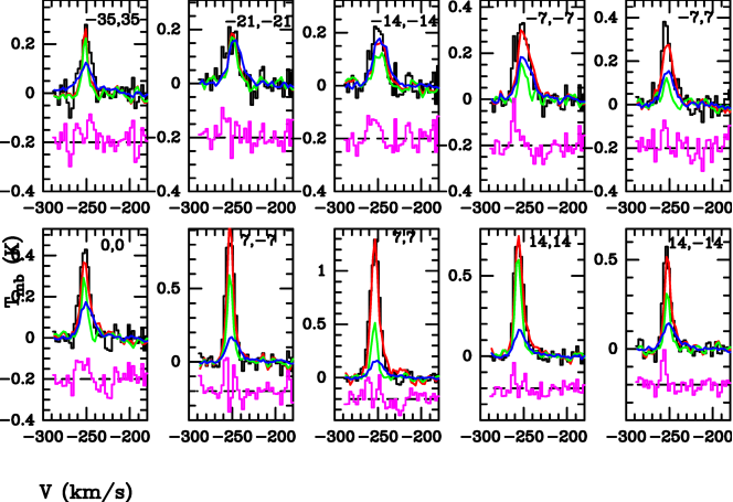
Figure 9: [C ii] (black), CO(2–1) (green), and H i (blue) spectra at selected positions in the BCLMP302 region. The H i spectrum has been scaled by a factor of 0.002 for easier comparison. The fit to the observed [C ii] spectrum, as obtained from the method described in text, is shown in red and the residual spectrum (vertically offset) is shown in magenta.

Table 3: Same as Table 2, but for selected positions in the BCLMP302 region.

Offset	$\upsilon_{\rm min}$	$\upsilon_{\rm max}$	$I$([C ii])	$I$(CO(2–1)	$N$(H i)	$I_{\rm res}$([C ii])	$\frac{I_{\rm res}(CII)}{I(CII)}$	$a$	$b$
(″,″)	km s-1	km s-1	K km s-1	K km s-1	1021cm-2	K km s-1
(-35, 35)	-268	-237	3.42$\pm$0.45	1.6	2.0	1.09	0.32	1.0	6.7e-4
(-21,-21)	-276	-232	3.49$\pm$0.50	2.3	2.7	0.81	0.23	1.0	2.3e-4
(-14,-14)	-270	-233	3.90$\pm$0.48	2.0	3.2	0.70	0.18	0.7	1.0e-3
( -7, -7)	-272	-227	6.12$\pm$0.57	1.7	3.4	0.44	0.07	0.3	2.8e-3
( 0, 0)	-268	-228	6.09$\pm$0.39	2.7	2.8	0.66	0.11	0.8	2.2e-3
( 7, 7)	-274	-227	17.61$\pm$0.55	4.5	2.7	1.12	0.06	1.7	5.9e-3
( 14, 14)	-269	-237	9.93$\pm$0.41	6.1	2.4	0.50	0.05	0.8	3.7e-3
( 14,-14)	-274	-233	5.93$\pm$0.45	2.5	2.3	0.44	0.07	1.3	1.8e-3

Figure 9 shows the observed [C ii], CO(2–1) and H i spectra (all smoothed to 2.6 km s^-1) for ten selected positions in the BCLMP302 region, along with the fit to the spectrum at each position derived using the described method and the residual spectrum. We find that (as mentioned before) the [C ii] spectrum has a line width intermediate between the CO(2–1) and H i spectra and the peak velocity of [C ii] is slightly shifted. However, unlike the [C ii] spectrum from the central region, in BCLMP302 the spectral profiles of [C ii], CO(2–1) and H i look similar with very little [C ii] emission detected at velocities not detected in the other two tracers. This is different from the conclusions derived on the basis of the integrated intensity maps of the region (Fig. 3), which show very little similarity in the emission features due to the three tracers. We performed fits to the spectra at all positions in the BCLMP302 region following the procedure presented above and find that the contribution of the gas not traced by either CO(2–1) and H i ranges between 10-55%, with typical values around 20% (Table 3).

7 Emission of [C ii] of ionized gas

In order to investigate the origin of [C ii] intensity not directly assignable to the observed CO(2–1) and H i emission, we estimate the possible contribution of H ii regions in the center and in BCLMP302. Among the H ii regions observed by Israel & van der Kruit (1974), the H ii regions # 35, 37, 38, and 42 are located in the central region and #53 corresponds to BCLMP302.

The relation between the [C ii] intensity (in K km s^-1) and the column density, $N$(C⁺) is (Crawford et al. 1985; Pineda et al. 2013)

$$I({\mathrm{C}II})=N({\mathrm{C}^{+}})\left[3.05\times 10^{15}\left(1+0.5\left(1+\frac{A_{ul}}{qn}\right)\exp^{91.2/kT_{\rm kin}}\right)\right]^{-1},$$ (2)

where $A_{\rm ul}=2.3\times 10^{6}$ s^-1 is the Einstein spontaneous decay rate and $q$ is the collisional de-excitation rate coefficient at a kinetic temperature of $T_{\rm kin}$. We assume $n=100$ cm^-3 and $T_{\rm kin}$ = 10000 K (typical for H ii regions). For collisions between C⁺ and electrons the de-excitation coefficient $q$ = 1.4$\times 10^{-6}$T${}_{\rm kin}^{-0.37}$ = 4$\times 10^{-8}$ s^-1 cm^-3 (Goldsmith et al. 2012). Thus we get $I$([C ii]) [K km s^-1]= $N$(C⁺)/5.5$\times 10^{15}$. We use the emission measure (EM = $n_{e}^{2}D$, where $D$ is the size of the source) observed by Israel & van der Kruit (1974) to determine $N$(H) (assuming H to be completely ionized, $n_{e}$ = $n$(H⁺) and $N$(H⁺)=$N$(H)=$n$(H)$D$) for $n$=100 cm^-3. Since the metallicity of M 33 as determined by Magrini et al. (2010) does not vary significantly within the inner 2.5 kpc, we use C/H = 8$\times 10^{-5}$ (assuming no depletion, since to a good approximation there are no grains in H ii regions) to estimate $N_{\rm ion}$(C⁺) from $N$(H) for all H ii regions.

Table 4: Estimate of [C ii] emission from ionized gas.

#	($\Delta\alpha$,$\Delta\delta$)	EM	$N$(H)	$N_{\rm ion}$(C+)	$I_{\rm ion}$(CII)
		103	1020	1016
	(″,″)	pc cm-6	cm-2	cm-2	K km s-1
Center
35	(-15,-37)	3.0	0.93	0.74	1.3a
37	(0,0)	19.1	5.9	4.7	2.1b
38	(16,23)	5.2	1.6	1.3	1.7
42	(62,4)	3.6	1.1	0.89	1.6
BCLMP302
53	(7,7)	3.0	0.93	0.74	1.3

^a $I$(CII) at (-15,-37) is 11.4 K km s^-1.
^b Using a dilution factor of 0.20 to account for the smaller size of the H ii region (5$\aas@@fstack{\prime\prime}$4) compared to the 12″ resolution of [C ii] data.

Table 4 presents the parameters for the four H ii regions as obtained from Israel & van der Kruit (1974), along with estimates of the [C ii] intensity originating from the ionized gas. We emphasize that only the H ii region #37 is smaller (5$\aas@@fstack{\prime\prime}$4) than the HIFI beamsize and the $I$([C ii]) estimated to arise from the ionized gas had to be corrected for the beam dilution. For the positions in the central region: at (-15,-37), (0,0), (16,23), and (62,4) the ionized gas contributes 11%, 25%, 18%, and 10% respectively, to the total [C ii] emission. In BCLMP302, we find that while 14% of [C ii] emission is unexplained at (7,7), only 7% can arise from the ionized gas. Mookerjea et al. (2011) had used the measured [N ii] (122 $\mu$m) intensities to estimate a contribution of 20–30% by the ionized gas in BCLMP302. Both of these estimates depend crucially on the value assumed for $n_{\rm e}$. For smaller values of $n_{\rm e}$ the contribution of the ionized gas to the [C ii] intensity is larger, as less Carbon is driven to higher ionization states (Abel 2006). In the present estimate, as well as in Mookerjea et al. (2011), a density of $n_{\rm e}$ = 100 cm^-3 has been used and the contribution of ionized gas to the overall [C ii] emission is found to be $<$25% in the two regions of M 33.

8 Properties of the neutral atomic gas emitting [C ii]

We use the results of the fitting procedure to estimate the fraction of [C ii] emission arising from the molecular gas traced by CO(2–1) and atomic gas traced by H i (Tables 5 and 6). Kramer et al. (2013) had estimated that for positions along the major axis of M 33, PDRs contribute a constant H i column density of 3.25$\times$10²⁰ cm^-2, which is 15–70% of the total H i column density they observed. They had concluded that diffuse atomic clouds (the cold neutral medium) contribute $\sim$15% of the observed [C ii] emission in the inner 2 kpc of M 33, while this contribution rises to about 40% in the outer disk at 6 kpc. Here for the central and BCLMP302 regions the observed $N$(H i) lies between 9.0$\times$10²⁰ cm^-2 and 3.4$\times$10²¹ cm^-2, so that the PDR contribution to the H i intensity lies at 10–30%. The typical H i column density of diffuse atomic clouds is $<$few$\times$10²⁰ cm^-2, while that for the atomic envelopes of dense molecular clouds lie in the range (1-7)$\times 10^{20}$ cm^-2 (Wolfire et al. 2010). This suggests that the observed H i emission either arises from several diffuse clouds or from the atomic envelopes of dense molecular clouds, which also emit in [C ii]. This is consistent with Kramer et al. (2013) and the results of the Galactic [C ii] survey by Langer et al. (2014), which had concluded that the H i emission is much brighter than what is expected from a single diffuse atomic cloud.

It is not possible to separate out the contribution of the diffuse and dense (PDR) atomic gas based on velocity information. However, since the PDR contribution to H i intensity is less than 30% for the two regions considered here, we use the total H i intensities for the following calculations. We use the fraction of [C ii] intensity estimated in the fits (Sec. 6) to arise from the atomic gas (Tables 5 and 6), the observed $N$(H i) (Tables 2 and 3) and Eq. (2) to estimate the volume density ($n$(H i)) of atomic gas, which could account for the [C ii] emission. We assume the temperature of the atomic gas to be 100 K and at this temperature the de-excitation coefficient for C⁺-H collisions is 8.1$\times 10^{-10}$ s^-1 cm^-3 (Launay & Roueff 1977). For the atomic gas, we estimate that 50% of the carbon is locked in the dust grains so that the C/H ratio is half the value used for the ionized gas; C/H = 4$\times 10^{-5}$. We find that at most positions in the center the atomic gas densities are larger than 200 cm^-3 and go up to 1700 cm^-3 at the position of the brightest H ii region (Table 5). Similarly, in the BCLMP302 region the atomic gas densities are larger than 150 cm^-3 and go up to 1500 cm^-3. Thus the H i gas contributing to the [C ii] emission has densities significantly larger than the densities found in diffuse clouds and are most likely to be atomic envelopes of molecular PDRs.

Table 5: Relative contribution of CO(2–1) and H i emitting molecular and atomic gas to [C ii] emission at positions in the central region of M 33 $I_{\rm CO}$(CII) and $I_{\rm HI}$(CII) are the estimated integrated intensities of [C ii] obtained from the fits described in the text. The difference between the observed [C ii] intensity and the result of this fit is $I_{\rm res}$(CII).

Offset	$\frac{I_{\rm CO}(CII)}{I(CII)}$	$\frac{I_{\rm HI}(CII)}{I(CII)}$	$\frac{I_{\rm res}(CII)}{I(CII)}$	$n$(H i)
(″,″)	%	%	%	cm-3
(-21, 38)	11	51	38	590
(-12,-28)	9	42	49	670
(-8,-19)	9	31	60	520
(-4,-9)	18	44	38	1700
( 0,0)	29	48	23	690
( 4,9)	57	16	27	230
( 7,27)	32	15	53	270
( 8,19)	33	8	59	100
(12,28)	31	9	60	160
(16,23)	28	9	63	150
(62,4)	53	36	11	1500
(71,0)	45	18	37	310

Table 6: Same as Table 5, but for positions in the BCLMP302 region.

Offset	$\frac{I_{\rm CO}(CII)}{I(CII)}$	$\frac{I_{\rm HI}(CII)}{I(CII)}$	$\frac{I_{\rm res}(CII)}{I(CII)}$	$n$(H i)
(″,″)	%	%	%	cm-3
(-35, 35)	47	21	32	104
(-21,-21)	67	10	23	34
(-14,-14)	37	45	18	160
(-7,-7)	7	86	7	532
( 0,0)	34	55	11	383
( 7,7)	43	51	6	1540
(14,14)	46	49	5	740
(14,-14)	54	39	7	316

9 Estimate of carbon abundances at selected positions

We next check the consistency of the derived column densities of C⁺, C⁰, and CO with the abundance of gaseous carbon relative to hydrogen. To accomplish this, we select two positions, one each in the two regions presented here, for which we also have low-$J$ CO (¹³CO) observations at an angular resolution similar to the [C ii] observations.

For GMC1 (Gratier et al. 2012), a molecular cloud in the central region (offset 62″,4″), an LTE analysis of the CO (and ¹³CO) intensities of the $J$=1–0 and $J$=2–1 was performed by Buchbender et al. (2013). For the BCLMP302 region, Mookerjea et al. (2011) have presented the CO(¹³CO) intensities based on IRAM 30m observations at a position almost coincident with the offset (7″,7″). The fraction of [C ii] emission contributed by the molecular, atomic, and gas unassociated with CO and H i emission in GMC1 is 53%, 36%, and 11%. In BCLMP302 it is 43%, 51%, and 6%. The H ii region contributes 11% and 7% of the total [C ii] emission in GMC1 and BCLMP302, respectively. The density of atomic gas required to explain the fraction of [C ii] emission arising from it is 1500 cm^-3 for both positions.

For both positions, we estimate the CO column densities from the ¹³CO(1–0) intensities assuming LTE and optically thin emission

$$N=\frac{3h}{8\pi^{3}S\mu^{2}}\frac{Z}{g_{J}}\frac{\exp{\left(\frac{h\nu}{kT_{\rm ex}}\right)}}{\left[\exp{\left(\frac{h\nu}{kT_{\rm ex}}\right)-1}\right]}\left[J_{\nu}(T_{\rm ex})-J_{\nu}(T_{\rm BG})\right]^{-1}\int{T_{\rm mb}d\upsilon},$$ (3)

where $\mu$ = 0.11 Debye is the dipole moment for CO, $S=J/(2J+1)$ is the line strength, $Z$ = $\sum\limits_{J=0}^{\infty}g_{J}\exp\left(-\frac{E_{J}}{kT}\right)$ is the partition function, $E_{J}$ = $hBJ(J+1)$, $g_{J}=(2J+1)$, $J_{\nu}(T)=\frac{h\nu}{k}\frac{1}{\exp^{{h\nu}/kT}-1}$. We assume the excitation temperatures (T_ex) to be the same as the dust temperatures at the selected positions and use the values given by Buchbender et al. (2013). For GMC1 we use the $I$(CO(1–0)) from Table 2 of Buchbender et al. (2013), $I$(CO(2–1)) from this work and for position (7,7) in BCLMP302, we use Table 2 of Mookerjea et al. (2011).

Next for the CO(1–0) and (2–1) intensities, we use the abovementioned excitation temperatures as kinetic temperatures and the estimated LTE column densities to estimate the local volume densities ($n$) based on an LVG analysis using RADEX (van der Tak et al. 2007). The values of $n$ at GMC1 and BCLMP302 are 3.3$\times 10^{3}$ cm^-3 and 9$\times 10^{3}$ cm^-3, respectively. For these densities ($n$), we assume a kinetic temperature of 91 K and use for the C⁺-H₂ collisions de-excitation coefficients given by $q=\left(4.9+0.22\frac{T_{\rm kin}}{100K}\right)\times 10^{-10}$ (Eq. 3 in Wiesenfeld & Goldsmith 2014) to estimate $N$(C⁺) at the selected positions using Eq. 2. Table 7 presents the parameters and estimated C⁺ and CO column densities for the two positions in the center and BCLMP302 region. We find that the two positions have very similar values of $N$(C⁺), although GMC1 has a $N$(CO), which is three times higher than the value of the BCLMP302 position. The BCLMP302 position, on the other hand has a 1.6 times higher atomic hydrogen column density. In low metallicity galaxies like the SMC and LMC recent observations have shown that [C i] has a column density similar to or within a factor of 4 of the CO column density (Okada et al. 2015, Requena-Torres et al in prep.). In the absence of [C i] observations, we assume that $N$(CO) = $N$(C⁰) and calculate the total carbon column density, $N$(C), at the two selected positions as $N$(C⁺)+$N$(C⁰)+$N$(CO).

Braine et al. (2010) derived a H₂ column density map for M 33 based on the 500 $\mu$m SPIRE map, $\beta=2$ and the 250/350 $\mu$m dust temperature. These authors proposed that within the inner 2 kpc of M 33 the $N$(H₂) scales as 2.2$\times 10^{20}I$(CO(2–1)). For the two selected positions we estimate $N$(H₂) with this scaling relation and the measured $I$(CO(2–1)) (Table 7). The total hydrogen column density ($N_{\rm tot}$ = $N$(H)+2$N$(H₂)) at both these positions results to 5.1$\times$10²¹ cm^-2. Thus we estimate the abundance of carbon in the center and in the BCLMP302 region to be 5.6$\times 10^{-5}$ and 4.1$\times 10^{-5}$ and it is consistent with our assumption of 50% depletion of carbon onto the grains.

Table 7: Estimate of column densities .

Position	$I$(CO(1–0))	$I$(CO(2–1))	$I$(13CO(1–0))	$T_{\rm ex}^{a}$	$N$(CO)b	$n$(H2)c	$N$(C+)d	$N$(H2)e	$N$(H i)f
	K km s-1	K km s-1	K km s-1	K	1016cm-2	cm-3	1017cm-2	1021cm-2	1021cm-2
Center
(62,4)	7.2	7.7	0.799	25	8.3	3300	2.0	1.7	1.7
BCLMP302
(7,7)	3.2	5.3	0.28	22	3.1	9000	1.6	1.2	2.7

^a Equal to the $T_{\rm dust}$ as in Table D.1 of Buchbender et al. (2013).
^b Calculated from $I$(¹³CO(1–0)), $T_{\rm ex}$ and ${12}$C/¹³C = 60.
^c Estimated from LVG analysis of CO(1–0) and CO(2–1) intensities, with $T_{\rm dust}$ as T_kin and $N$(CO) as inputs.
^d Estimated using $n$ derived from $I$(CO(1–0)) and $I$(CO(2–1)) using LVG model, $T_{\rm ex}$ = 91 K and $I$([C ii]) in Tables 2 & 3 in Eq. 2.
^e Estimated using $N$(H₂) = 2.2$\times 10^{20}$ $I$(CO(2–1)) (Braine et al. 2010).
^f See Tables 2 and 3.

10 Discussion

10.1 Phases of ISM contributing to [C ii] emission

One of the primary aims of the HerM 33es project has been to disentangle the contribution of the different phases of the ISM toward [C ii] emission in M 33. In this paper, we have used velocity-resolved [C ii] spectra to estimate the contributions of dense PDRs (traced by CO(2–1)), atomic gas (dense and diffuse), ionized gas, and the CO-dark molecular gas to the observed [C ii] emission. In the two regions of M 33 studied here, we find that the contributions of the molecular gas traced by CO and atomic gas traced by H i to the [C ii] intensity vary substantially from position to position. The contribution of the ionized gas to the [C ii] intensity is estimated to be typically between 10–20%. For the Milky Way, the ISM components have been shown to have approximately comparable contributions to the [C ii] luminosities: dense PDRs (30%), cold H i (25%), CO-dark H₂ (25%), and ionized gas (20%) (Pineda et al. 2014). Furthermore, Pineda et al. (2013) concluded that the fraction of the CO-dark molecular gas traced by [C ii] ranges from about 20% in the metal-rich inner Galaxy to 80% in the metal poor outer-Galaxy. M 33 has approximately half the solar metallicity and in the outskirts of the Galactic disk the metallicity is comparable to the metallicity of M 33. In addition to being at a metallicity twice the value of M 33, these observations of the long lines of sight through the Galactic disk are sensitive to significant contributions from the diffuse gas and, hence, may not be directly comparable to the observations of M 33. Recent SOFIA observations of regions in the SMC and LMC are probably more directly comparable to the case of M 33. In the star-forming regions of the SMC at a resolution of 10 pc, the [C ii] emission is found to trace between 50–85% of the bulk of the mass of the molecular gas, with minor contributions from the ionized gas in the H ii regions (Requena-Torres et al. in prep.). For N159 in the LMC, Okada et al. (2015) concluded that the fraction of the [C ii] emission that cannot be attributed to the material traced by the CO line profiles, is around 20% around the CO cores and up to 50% in the area between the cores. In M 33, though we do not have the spatial resolution to distinguish the core and inter-core regions, the fraction of [C ii] intensity tracing the CO-dark molecular gas is similar to the value found in the LMC. In the LMC, the ionized gas contributes $\sim 15$% of the [C ii] emission, which is similar to our estimate of 10–20% for the two regions in M 33.

10.2 Emission of [C ii] unassociated with CO or H i

Use of high spectral resolution observations has led to the detection of significant [C ii] intensity from molecular gas not detected in CO(2–1). Such excess [C ii] emission has been observed along many Galactic lines of sight (Pineda et al. 2013, and references therein), as well as in external galaxies including the SMC and LMC (Madden et al. 1997; Okada et al. 2015, Requena-Torres et al in prep.). A possible explanation is that this excess [C ii] emission is produced in the envelopes of dense molecular clouds in which the H i/H₂ transitions are largely complete, but the column densities are low enough such that the C⁺/C⁰/CO transition is still far from complete. Wolfire et al. (2010) theoretically estimated that the mass fraction of CO-dark molecular gas increases with decreasing $A_{\rm V}$, since relatively more molecular H₂ material lies outside the CO region in this case. For M 33 we estimate the fraction of [C ii] intensity without any corresponding CO(2–1) and H i emission to be between 20–60% in the central region and below 30% in the BCLMP302 region. This difference in the estimated fraction of CO-dark molecular gas toward [C ii] emission in two regions of M 33 could be due to the difference in the FUV flux, extinction, and metallicity. Since within the inner 2 kpc of M 33 the metallicity does not vary significantly (Magrini et al. 2007), we compare the FUV intensities and extinction in the two regions next.

For stars embedded in dusty clouds, the total FUV photon energy deposited into the cloud is re-emitted in the FIR, hence the FUV intensity varies linearly as the total FIR continuum intensity (Kaufman et al. 1999). Thus to estimate the FUV intensity we first estimated the total FIR continuum intensity in the central and BCLMP302 regions from the PACS 70, 100, and 160 micron intensities. For M 33, Xilouris et al. (2012) found that a modified blackbody with $\beta=1.5$ and warm dust temperatures of the order of 55 K provide the best fit. Using these parameters Nikola et al. (in prep) estimated that the total FIR intensities for the two regions in M 33 studied here have similar values with peaks of 2–3 10^-15 Watt m^-2 pixel^-1 for a 3″ pixel. The similarity in range of FIR intensities in the two regions indicate similar values of the far ultraviolet (FUV) intensities for the two regions.

Based on the 24 $\mu$m MIPS and the H$\alpha$ maps for M 33, an extinction map for the entire galaxy was generated by Monica Relano (priv. comm) via the method presented by Relaño & Kennicutt (2009). The $A_{\rm V}$ thus calculated are similar for the central and BCLMP302 regions, with typical values between 0.6–0.7 mag. At the position of the [C ii] peak in BCLMP302 the value of $A_{\rm V}$ is 0.4 mag. At the location of the [C ii] peaks in the central region, $A_{\rm V}$ ranges between 0.5–1.6. The somewhat higher values of $A_{\rm V}$ seen toward the center also does not help us explain the larger proportion of CO-dark molecular H₂ at the center. The $A_{\rm V}$ values presented here are averaged over a 12″ beam. Given the inhomogeneous nature of the ISM, it is likely that the actual value of $A_{\rm V}$ on smaller spatial scales is significantly larger than the average estimated.

Thus at a resolution of 50 pc the difference in metallicity, FUV radiation field, and extinction between the center and the BCLMP302 regions are not significant enough to explain the difference in the CO-dark component of molecular gas. This indicates a variation of the relative amounts of diffuse (CO-dark) and dense molecular gas on spatial scales smaller than 50 pc.

10.3 Interpretation of correlation between [C ii], CO, and H i

We find that the derived correlation between [C ii], CO and H i intensities depends crucially on the availability of spectral and spatial resolution. Velocity-resolved spectra for BCLMP302 show very little [C ii] emission not associated with CO and H i. However, H i and CO are spatially disjunct and integrated intensities without velocity information mix [C ii] contributions from H i and CO. Thus, we find a low correlation between [C ii] and either of them when looking at just the integrated intensities. When we are able to filter out CO and H i gas based on the velocity information, we obtain a much better correlation (Table 1) as we only compare contributions corresponding to the same velocity ranges. For the center, we estimate a large amount of nonassociated [C ii] emission leading to a low correlation when we are able to determine the associations based on the velocity information, as reflected by the lower numbers in Table 1. The higher correlation when considering integrated intensities (Fig. 5) must indicate a spatial relation of the CO-dark [C ii] emitting molecular gas to the other tracers. Thus, for the central region, a possible explanation of the derived correlations could be in terms of production of the excess [C ii] emission in gas falling onto or outflowing from denser CO gas. These results show the complementarity of information provided by observations with or without spectral resolution, which needs to be factored in when interpreting observed correlations or the lack of it as seen in galaxies at larger distances.

11 Summary

A comparison of velocity-resolved observations of [C ii] with other dedicated tracers of neutral atomic and molecular gases has been used to find the relative contribution of the atomic and molecular phases of the ISM at all positions in two regions within the Triangulum galaxy M 33. The difference in the estimated [C ii] emission that is not originating from CO(2–1) and H i emitting clouds, between the center and the BCLMP302 regions does not have any obvious explanation in terms of the variation of extinction, FUV radiation field, and metallicity of the gas at spatial scales of 50 pc. This suggests the role of smaller scale variations of all these parameters toward the observed [C ii] emission. Based on detailed analysis of one position each in the center and in the BCLMP302 regions, we estimate that 70% and 89% of gas-phase carbon is in the form of C⁺. In both these regions at selected locations coinciding with H ii regions, 10–20% of the [C ii] intensities arise from the ionized gas. However in the absence of any velocity information about the ionized gas it is not possible to conclude whether this could explain at least part of the [C ii] emission not corresponding to the H i and CO(2–1) emission. While the velocity information and better spatial (50 pc) resolution significantly improves our understanding of the origin of [C ii] in emission, even from nearby extragalactic sources, such as M 33, where the linear resolution in the present observations is 50 pc, the situation is still complicated by the intermixing of emission from different physical entities within the same beam.