Estimating Learning Effects: A Short-Time Fourier Transform Regression Model for MEG Source Localization

Abstract

Magnetoencephalography (MEG) has a high temporal resolution well-suited for studying perceptual learning. However, to identify where learning happens in the brain, one needs to apply source localization techniques to project MEG sensor data into brain space. Previous source localization methods, such as the short-time Fourier transform (STFT) method by Gramfort et al.([Gramfort et al., 2013]) produced intriguing results, but they were not designed to incorporate trial-by-trial learning effects. Here we modify the approach in [Gramfort et al., 2013] to produce an STFT-based source localization method (STFT-R) that includes an additional regression of the STFT components on covariates such as the behavioral learning curve. We also exploit a hierarchical $L_{21}$ penalty to induce structured sparsity of STFT components and to emphasize signals from regions of interest (ROIs) that are selected according to prior knowledge. In reconstructing the ROI source signals from simulated data, STFT-R achieved smaller errors than a two-step method using the popular minimum-norm estimate (MNE), and in a real-world human learning experiment, STFT-R yielded more interpretable results about what time-frequency components of the ROI signals were correlated with learning.

This is an author manuscript. The paper is in press and will be published in the volume for the 4th NIPS Workshop on Machine Learning and Interpretation in Neuroimaging (2014), Lecture Notes in Computer Science, Springer. (Original publication link by Springer will appear here later.)

1 Introduction

Magnetoencephalography (MEG) [Hamalainen et al., 1993] has a high temporal resolution well-suited for studying the neural bases of perceptual learning. By regressing MEG signals on covariates, for example, trial-by-trial behavioral performance, we can identify how neural signals change with learning. Based on Maxwell’s equations[Hamalainen and Ilmoniemi, 1994], MEG sensor data can be approximated by a linear transform of the underlying neural signals in a “source space”, often defined as $\sim 10^{4}$ source points distributed on the cortical surfaces. Solving the inverse of this linear problem (“source localization”) facilitates identifying the neural sites of learning. However, this inverse problem is underspecified, because the number of sensors ($\sim 300$) is much smaller than the number of source points. Many source localization methods use an $L_{2}$ penalty for regularization at each time point (minimum-norm estimate [Hamalainen and Ilmoniemi, 1994], dSPM [Dale et al., 2000] and sLORETA [Pascual-Marqui, 2002]). These methods, however, may give noisy solutions in that they ignore the temporal smoothness of the MEG signals. Other methods have been proposed to capture the temporal structure (e.g. [Galka et al., 2004, Lamus et al., 2012]), among which, a sparse short-time Fourier transform (STFT) method by Gramfort et al. [Gramfort et al., 2013] yields solutions that are spatially sparse and temporally smooth.
With $L_{2}$ methods such as the minimum-norm estimate (MNE), one can study learning effects in a two-step procedure: 1) obtain source time series in each trial; 2) regress some features of the time series on the covariates. However, these methods may give noisy solutions due to lack of smoothness. To address this, we might want to regress the STFT components in [Gramfort et al., 2013] on the covariates in a two-step procedure, but being designed for single-trial data, [Gramfort et al., 2013] may not provide consistent sparse structures across trials. Additionally, in cases with pre-defined regions of interest (ROIs) that are theoretically important in perceptual learning, for example, “face-selective” areas [Gauthier et al., 2000, Kanwisher et al., 1997, Pitcher et al., 2011], it is not desirable to shrink all source points equally to zero as in MNE. Instead, it may be useful to assign weighted penalties to emphasize the ROIs.
Here we modify the model in [Gramfort et al., 2013] to produce a new method (STFT-R) to estimate learning effects in MEG. We represent the source signals with STFT components and assume the components have a linear relationship with the covariates. To solve the regression coefficients of STFT components, we design a hierarchical group lasso ($L_{21}$) penalty [Jenatton et al., 2011] of three levels to induce structured sparsity. The first level partitions source points based on ROIs, allowing different penalties for source points within ROIs and outside ROIs; then for each source point, the second level encourages sparsity over time and frequency on the regression coefficients of the STFT components, and finally for each STFT component, the third level induces sparsity over the coefficients for different covariates. We derive an algorithm with an active-set strategy to solve STFT-R, and compare STFT-R with an alternative two-step procedure using MNE on both simulated and human experimental data.

2 Methods

Model Assume we have $n$ sensors, $m$ source points, $T$ time points in each trial, and $q$ trials together. Let $\bm{M}^{(r)}\in\mathbb{R}^{n\times T}$ be the sensor time series we observe in the $r$th trial, and $\bm{G}\in\mathbb{R}^{n\times m}$ be the known linear operator (“forward matrix”) that projects source signals to sensor space. Following the notation in [Gramfort et al., 2013], let $\bm{\Phi^{H}}\in\mathbb{C}^{s\times T}$ be $s$ pre-defined STFT dictionary functions at different frequencies and time points (see Appendix 1). Suppose we have $p$ covariates (e.g. a behavioral learning curve, or non-parametric spline basis functions), we write them into a design matrix $\bm{X}\in\mathbb{R}^{q\times p}$, which also includes an all-one column to represent the intercept. Besides the all one column, all other columns have zero means. Let the scalar $X_{k}^{(r)}=\bm{X}(r,k)$ be the $k$th covariate in the $r$th trial. When we represent the time series of the $i$th source point with STFT, we assume each STFT component is a linear function of the $p$ covariates: the $j$th STFT component in the $r$th trial is $\sum_{k=1}^{p}X_{k}^{(r)}Z_{ijk}$, where the regression coefficients $Z_{ijk}$’s are to be solved. We use a complex tensor $\bm{Z}\in\mathbb{C}^{m\times s\times p}$ to denote the $Z_{ijk}$’s, and use $\bm{Z}_{k}\in\mathbb{C}^{m\times s}$ to denote each layer of $\bm{Z}$. Our STFT-R model reads

$$\bm{M}^{(r)}=\bm{G}\left(\sum_{k=1}^{p}X_{k}^{(r)}\bm{Z_{k}}\right)\bm{\Phi^{H}}+\bm{E}^{(r)}\hskip 10.00002pt\text{ for }\hskip 10.00002ptr=1,\cdots,q.$$

where the error $\bm{E}^{(r)}\in\mathbb{R}^{n\times T}$ is an i.i.d random matrix for each trial. To solve $\bm{Z}$, we minimize the sum of squared prediction error across $q$ trials, with a hierarchical $L_{21}$ penalty $\Omega$ on $\bm{Z}$:

$$\min_{\bm{Z}}\left(\frac{1}{2}\sum_{r=1}^{q}\|\bm{M}^{(r)}-\bm{G}(\sum_{k=1}^{p}X_{k}^{(r)}\bm{Z}_{k})\bm{\Phi^{H}}\|_{F}^{2}+\Omega(\bm{Z},\alpha,\beta,\gamma,\bm{w})\right)$$ (1)

where $\|\cdot\|_{F}$ is the Frobenius norm and

$$\Omega(\bm{Z},\alpha,\beta,\gamma,\bm{w}) =\alpha\sum_{l}w_{l}\sqrt{\sum_{i\in\mathcal{A}_{l}}\sum_{j=1}^{s}\sum_{k=1}^{p}|Z_{ijk}|^{2}}$$ (2)

$$+\beta\sum_{i=1}^{m}\sum_{j=1}^{s}\sqrt{\sum_{k=1}^{p}|Z_{ijk}|^{2}}$$ (3)

$$+\gamma\sum_{i=1}^{m}\sum_{j=1}^{s}\sum_{k=1}^{p}|Z_{ijk}|.$$ (4)

The penalty $\Omega$ involves three terms corresponding to three levels of nested groups, and $\alpha$, $\beta$ and $\gamma$ are tuning parameters. On the first level in (2), each group under the square root either consists of coefficients for all source points within one ROI, or coefficients for one single source point outside the ROIs. Therefore we have $N_{\alpha}$ groups, denoted by $\mathcal{A}_{l},l=1,\cdots,N_{\alpha}$, where $N_{\alpha}$ is the number of ROIs plus the number of source points outside the ROIs. Such a structure encourages the source signals outside the ROIs to be spatially sparse and thus reduces computational cost. With a good choice of weights for the $N_{\alpha}$ groups, $\bm{w}=(w_{1},w_{2},\dots w_{N_{\alpha}})^{T}$, we can also make the penalty on coefficients for source points within the ROIs smaller than that on coefficients for source points outside the ROIs. On the second level, for each source point $i$, the term (3) groups the $p$ regression coefficients for the $j$th STFT component under the square root, inducing sparsity over time points and frequencies. Finally, on the third level, (4) adds an $L_{1}$ penalty on each $Z_{ijk}$ to encourage sparsity on the $p$ covariates, for each STFT component of each source point.
The FISTA algorithm We use the fast iterative shrinkage-thresholding algorithm (FISTA [Beck and Teboulle, 2009]) to solve (1), with a constant step size, following [Gramfort et al., 2013]. Let $\bm{z}$ be a vector that is concatenated by all entries in $\bm{Z}$, and let $\bm{y}$ be a vector of the same size. In each FISTA step, we need the proximal operator associated with the hierarchical penalty $\Omega$:

$$\arg\min_{\bm{z}}(\frac{1}{2}\|\bm{z}-\bm{y}\|^{2}+\Omega(\bm{z},\alpha,\beta,\gamma,\bm{w}))=\arg\min_{\bm{z}}(\frac{1}{2}\|\bm{z}-\bm{y}\|^{2}+\sum_{h=1}^{N}\lambda_{h}{\|\bm{z}|_{g_{h}}\|_{2}})$$ (5)

where we concatenate all of the nested groups on the three levels in $\Omega$ into an ordered list $\{g_{1},g_{2},\cdots,g_{N}\}$ and denote the penalty on group $g_{h}$ by $\lambda_{h}$. For example, $\lambda_{h}=\alpha w_{l}$ if $g_{h}$ is the $l$th group on the first level, $\lambda_{h}=\beta$ if $g_{h}$ is on the second level, and $\lambda_{h}=\gamma$ if $g_{h}$ is on in the third level. $\{g_{1},g_{2},\cdots,g_{N}\}$ is obtained by listing all the third level groups, then the second level and finally the first level, such that if $h_{1}$ is before $h_{2}$, then $g_{h_{1}}\subset g_{h_{2}}$ or $g_{h_{1}}\cap g_{h_{2}}=\emptyset$. Let $\bm{z}|_{g_{h}}$ be the elements of $\bm{z}$ in group $g_{h}$. As proved in [Jenatton et al., 2011], (5) is solved by composing the proximal operators for the $L_{21}$ penalty on each $g_{h}$, following the order in the list; that is, initialize $\bm{z}\leftarrow\bm{y}$, for $h=1,\cdots N$ in the ordered list,

$$\bm{z}|_{g_{h}}\leftarrow\left\{\begin{array}[]{l l}\bm{z}|_{g_{h}}(1-\lambda_{h}/\|\bm{z}|_{g_{h}}\|_{2})&\text{ if }\|\bm{z}|_{g_{h}}\|_{2}>\lambda_{h}\\ 0&\text{ otherwise }\end{array}\right.$$

Data: $L,f(\bm{z})=\frac{1}{2}\sum_{r=1}^{q}\|\bm{M}^{(r)}-\bm{G}\left(\sum_{k=1}^{p}X_{k}^{(r)}\bm{Z_{k}}\right)\bm{\Phi^{H}}\|_{F}^{2},\Omega(\bm{z})=\Omega(\bm{Z},\alpha,\beta,\gamma,\bm{w})$

Result: the optimal solution $\bm{z}$

initialization: $\bm{z_{0}},\zeta=1,\zeta_{0}=1$, $\bm{y}\leftarrow\bm{z_{0}}$, $\bm{z}\leftarrow\bm{z_{0}}$ ;

while  change of $\bm{z}$ in two iterations is not small enough  do

       $\bm{z_{0}}\leftarrow\bm{z}$; Compute $\nabla f(\bm{y})$ ;

       Apply the proximal operator $\bm{z}=\arg_{\bm{x}}\min(\frac{1}{2}\|\bm{x}-(\bm{y}-\frac{1}{L}\nabla f(\bm{y}))\|^{2}+\frac{1}{L}\Omega(\bm{x}))$;

       $\zeta_{0}\leftarrow\zeta$; $\zeta\leftarrow\frac{1+\sqrt{4\zeta_{0}^{2}+1}}{2}$; $\bm{y}\leftarrow\bm{z}+\frac{\zeta_{0}-1}{\zeta}(\bm{z}-\bm{z_{0}})$;

      

end while

Algorithm 1 FISTA algorithm given the Lipschitz constant $L$

Details of FISTA are shown in Algorithm 1, where $\bm{y}$ and $\bm{z_{0}}$ are auxiliary variables of the same shape as $\bm{z}$, and $\zeta,\zeta_{0}$ are constants used to accelerate convergence. The gradient of $f(\bm{z})$ is computed in the following way: $\frac{\partial f}{\partial\bm{Z}_{k}}=-\bm{G}^{T}\sum_{r=1}^{q}X_{k}^{(r)}\bm{M}^{(r)}\bm{\Phi}+\bm{G}^{T}\bm{G}(\sum_{r=1}^{q}X_{k}^{(r)}\sum_{k^{\prime}=1}^{p}\bm{Z}_{k^{\prime}}X_{k^{\prime}}(r))\bm{\Phi}^{H}\bm{\Phi}.$ We use the power iteration method in [Gramfort et al., 2013] to compute the Lipschitz constant of the gradient.
The active-set strategy In practice, it is expensive to solve the original problem in (1). Thus we derive an active-set strategy (Algorithm 2), according to Chapter 6 in [Bach et al., 2011]: starting with a union of some groups on the first level ($J=\cup_{l\in\mathcal{B}}{\mathcal{A}_{l}},\mathcal{B}\subset\{1,\cdots,N_{\alpha}\}$), we compute the solution to the problem constrained on $J$, then examine whether it is optimal for the original problem by checking whether the Karush-Kuhn-Tucker(KKT) conditions are met, if yes, we accept it, otherwise, we greedily add more groups to $J$ and repeat the procedure.
Let $\bm{z}$ denote the concatenated $\bm{Z}$ again, and let diagonal matrix $\bm{D}_{h}$ be a filter to select the elements of $\bm{z}$ in group $g_{h}$ (i.e. entries of $\bm{D}_{h}\bm{z}$ in group $g_{h}$ are equal to $\bm{z}|_{g_{h}}$, and entries outside $g_{h}$ are 0). Given a solution $\bm{z}_{0}$, the KKT conditions are

$$\nabla f(\bm{z})_{\bm{z}=\bm{z}_{0}}+\sum_{h}\bm{D}_{h}\bm{\xi}_{h}=0,\text{and}\begin{cases}\bm{\xi}_{h}=\lambda_{h}\frac{\bm{D}_{h}\bm{z}_{0}}{\|\bm{D}_{h}\bm{z}_{0}\|_{2}}&\text{if}\,\|\bm{D}_{h}\bm{z}_{0}\|_{2}>0,\\ \|\bm{\xi}_{h}\|_{2}\leq\lambda_{h}&\text{if}\,\|\bm{D}_{h}\bm{z}_{0}\|_{2}=0\end{cases}$$

where $\bm{\xi}_{h},h=1,\cdots,N$ are Lagrange multipliers of the same shape as $\bm{z}$. We defer the derivations to Appendix 2.
We minimize the following problem

$$\min_{\bm{\xi}_{h},\forall h}\frac{1}{2}\|\nabla f(\bm{z})_{\bm{z}=\bm{z}_{0}}+\sum_{h}\bm{D}_{h}\bm{\xi}_{h}\|_{2}^{2},$$

subject to $$\begin{cases}\bm{\xi}_{h}=\lambda_{h}\frac{\bm{D}_{h}\bm{z}_{0}}{\|\bm{D}_{h}\bm{z}_{0}\|_{2}}&\text{if}\,\|\bm{D}_{h}\bm{z}_{0}\|_{2}>0,\\ \|\bm{\xi}_{h}\|_{2}\leq\lambda_{h}&\text{if}\,\|\bm{D}_{h}\bm{z}_{0}\|_{2}=0\end{cases}$$

and use $\frac{1}{2}\|\nabla f(\bm{z})_{\bm{z}=\bm{z}_{0}}+\sum_{h}\bm{D}_{h}\bm{\xi}_{h}\|_{2}^{2}$ at the optimum to measure the violation of KKT conditions. Additionally, we use the $\frac{1}{2}\|\left(\nabla f(\bm{z})_{\bm{z}=\bm{z}_{0}}+\sum_{h}\bm{D}_{h}\bm{\xi}_{h}\right)|_{\mathcal{A}_{l}}\|_{2}^{2}$, constrained on each non-active first-level group $\mathcal{A}_{l}\not\subset J$, as a measurement of violation for the group.

initialization: choose initial $J$ and initial solution $Z$; compute the KKT violation for each $\mathcal{A}_{l}\not\in J$ ;

while  the total KKT violation is not small enough do

       add 50 non-active groups that have the largest KKT violations to $J$;

       compute a solution to the problem constrained on $J$ using FISTA ;

       compute the KKT violation for each $\mathcal{A}_{l}\not\subset J$ ;

      

end while

Algorithm 2 Active-set strategy

$\bm{L_{2}}$ regularization and bootstrapping The hierarchical $L_{21}$ penalty may give biased results [Gramfort et al., 2013]. To reduce bias, we computed an $L_{2}$ solution constrained on the non-zero entries of the hierarchical $L_{21}$ solution. Tuning parameters in the $L_{21}$ and $L_{2}$ models were selected to minimize cross-validated prediction error.
To obtain the standard deviations of the regression coefficients in $\bm{Z}$, we performed a data-splitting bootstrapping procedure. The data was split to two halves (odd and even trials). On the first half, we obtained the hierarchical $L_{21}$ solution, and on the second half, we computed an $L_{2}$ solution constrained on the non-zero entries of the hierarchical $L_{21}$ solution. Then we plugged in this $L_{2}$ solution $\bm{Z}$ to obtain residual sensor time series of each trial on the second half of the data ($\bm{R}^{(r)}=\bm{M}^{(r)}-\bm{G}(\sum_{k=1}^{p}X_{k}^{(r)}\bm{Z}_{k})\bm{\Phi^{H}}$). We rescaled the residuals according to the design matrix $\bm{X}$ [Stine, 1985]. Let $X_{r}=\bm{X}(r,:)^{T}=(X_{1}^{(r)},X_{2}^{(r)},\cdots,X_{p}^{(r)})^{T}$, and $h_{r}=X_{r}^{T}(\bm{X}^{T}\bm{X})^{-1}X_{r}$. The residual in the $r$th trial was rescaled by $1/(1-h_{r})^{0.5}$. The re-sampled residuals $\bm{R}^{(r)*}$s were random samples with replacement from $\{\bm{R}^{(r)}/(1-h_{r})^{0.5},r=1,\cdots,q\}$ and the bootstrapped sensor data for each trial were

$$\bm{M}^{(r)*}=\bm{G}(\sum_{k=1}^{p}X_{k}^{(r)}\bm{Z}_{k})\bm{\Phi^{H}}+\bm{R}^{(r)*}$$

After $B$ re-sampling procedures, for each bootstrapped sample, we re-estimated the solution to the $L_{2}$ problem constrained on the non-zero entries again, and the best $L_{2}$ parameter was determined by a 2-fold cross-validation.

3 Results

Simulation On simulated data, we compared STFT-R with an alternative two-step MNE method (labelled as MNE-R), that is, (1) obtain MNE source solutions for each trial; (2) apply STFT and regress the STFT components on the covariates.
We performed simulations using “mne-python” [Gramfort et al., 2014], which provided a sample dataset, and a source space that consisted of 7498 source points perpendicular to the gray-white matter boundary, following the major current directions that MEG is sensitive to. Simulated source signals were constrained in four regions in the left and right primary visual and auditory cortices (Aud-lh, Aud-rh, Vis-lh and Vis-rh, Fig. 1(a)). All source points outside the four regions were set to zero. To test whether STFT-R could emphasize regions of interest, we treated Aud-lh and Aud-rh as the target ROIs and Vis-lh and Vis-rh as irrelevant signal sources. The noiseless signals were low-frequency Gabor functions (Fig. 1(b)), whose amplitude was a linear function of a sigmoid curve (simulated “behavorial learning curve”, Fig. 1(c)). We added Gaussian process noise on each source point in the four regions independently for each trial. We denoted the ratio of the marginal standard deviation of this noise to the largest amplitude of the signal as noise levels, and ran multiple simulations with different noise levels. We also simulated the sensor noise as multivariate Gaussian noise filtered by a 5th order infinite impulse response (IIR) filter. The filter and covariance matrix of the sensor noise were estimated from the sample data. We used different signal-to-noise ratios (SNRs) in Decibel when adding sensor noise. Hence we had two different levels of noise characterized by noise level in the source space and SNR in the sensor space.
We ran 5 independent simulations for SNR $\in\{0.5,1\}$ and noise level $\in\{0.1,0.3,0.5\}$, with 20 trials (length of time series $T=100$, sampling rate = 100 Hz, window size of the STFT = $160$ ms and step size $\tau_{0}=40$ ms). With only one covariate (the sigmoid curve), we fit an intercept and a slope for each STFT component. Before applying both methods, we pre-whitened the correlation between sensors. In STFT-R, the weights for $\alpha$ in the ROI groups were set to zero, and the weights in the non-ROI groups were equal and summed to 1. We tuned the penalization parameters $\alpha$, $\beta$ in STFT-R. For $\gamma$, because the true slope and intercept were equal in the simulation, we did not need a large $\gamma$ to select between the slope and intercept, therefore we fixed $\gamma$ to a small value to reduce the time for parameter tuning. The $L_{2}$ penalty parameter in MNE-R was also selected via cross-validation. We used $B=20$ in bootstrapping.
We reconstructed the source signals in each trial using the estimated $\bm{Z}$. Note that true source currents that were close to each other could have opposite directions due to the folding of sulci and gyri, and with limited precision of the forward matrix, the estimated signal could have an opposite sign to the truth. Therefore we “rectified” the reconstructed signals and the true noiseless signals by taking their absolute values, and computed the mean squared error (MSE) on the absolute values. Fig. 1(d) shows estimated source signals in the target ROIs (red and yellow) by the two methods in the $20$th trial (SNR = 0.5, noise level = 0.5). Noticing the scales, we found that MNE-R shrank the signals much more than STFT-R. We show the ratios of the rectified MSEs of STFT-R to the rectified MSEs of MNE-R for source points within the ROIs (Fig. 1(e)), and for all source points in the source space (Fig. 1(f)). Compared with MNE-R, STFT-R reduced the MSE within the ROIs by about $20\sim 40\%$ (Fig. 1(e)) . STFT-R also reduced the MSE of all the source points by about $20\%$ in cases with low noise levels (0.1) (Fig. 1(f)). The MSE reduction was larger when noise level was small.

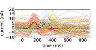
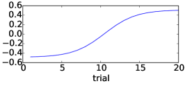
(a)	(b)	(c)

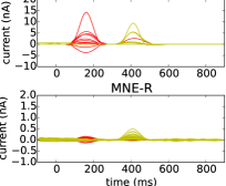
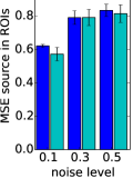
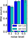
(d)	(e)	(f)

Figure 1: Simulation results: source signal reconstruction. (a), Target ROIs: Aud-lh (red), Aud-rh (yellow) and irrelevant regions: Vis-lh (blue), Vis-rh (green). (b), The simulated source signals with Gaussian process noise in the 20th trial. Each curve represents one source point. The thicker curves show the noiseless true signals (solid: target ROIs, dashed: irrelevant regions). noise level = 0.5. (c), The simulated “behavioral learning curve”. (d), Estimates of source signals (noise level = 0.5, SNR = 0.5) in the $20$th trial by STFT-R and MNE-R, in Aud-lh (red) and Aud-rh (yellow). Each curve represents one source point. Note the scale for MNE-R is $<1/10$ of the truth. (e) and (f), Ratios of rectified MSE (STFT-R over MNE-R) for source points within the target ROIs (e) and for all source points (f). The bars show averaged ratios across 5 independent runs of simulation, and the error bars show standard errors of the averaged ratios.

To visualize which time-frequency components were correlated with the covariate, we computed the T-statistic for each slope coefficient of each STFT component, defined as the estimated coefficient divided by the bootstrapped standard error. Again, since our estimate could have an opposite sign to the true signals, we rectified the T-statistics by using their absolute values. We first averaged the absolute values of the T-statistics for the real and imaginary parts of each STFT component, and then averaged them across all non-zero source points in an ROI, for each STFT component. We call these values averaged absolute Ts.
In Fig. 2, we plot the T-statistic of the slope coefficient for each STFT component of each source point in the two ROIs by STFT-R (Fig. 2(b)) and by MNE-R (Fig. 2(c)), and compared them with the true coefficients in Fig. 2(a) (SNR = 0.5, noise level = 0.5). The T-statistics for the real and imaginary parts are shown separately. In Fig. 2(a),(b) and (c), the vertical axis corresponds to the indices of source points, concatenated for the two ROIs. The horizontal axis corresponds to the indices of STFT components, which is a one-dimensional concatenation of the cells of the frequency $\times$ time matrix in Fig. 2(d); 0-24 are 25 time points in 0 Hz, 25-49 in 6.25 Hz, 50-74 in 12.5 Hz, and so on. STFT-R yielded a sparse pattern, where only the lower frequency (0 to 6.25 Hz) components were active, whereas the pattern by MNE-R spread into higher frequencies (index 100-200,25-50Hz). We also compared the averaged absolute Ts for each ROI by STFT-R (Fig. 2(e)) and by MNE-R (Fig. 2(f)), with the true pattern in Fig. 2(d), in which we averaged the absolute values of the real and imaginary parts of the true coefficients across the source points in the ROI. Again, STFT-R yielded a sparse activation pattern similar to the truth, where as MNE-R yielded a more dispersed pattern.

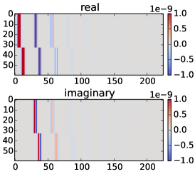
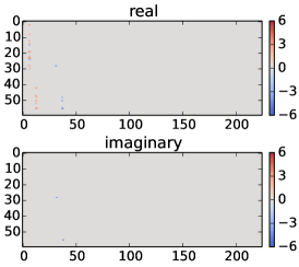
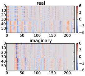
(a) Truth	(b) STFT-R	(c) MNE-R
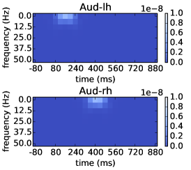
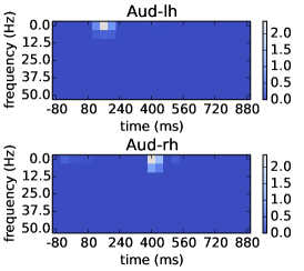
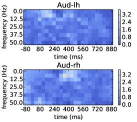
(d) Truth	(e) STFT-R	(f) MNE-R

Figure 2: Simulation results: inference of regression. SNR = 0.5, noise level = 0.5. (a), The true slope coefficients of the regression. The vertical axis corresponds to the indices of source points. Source points from the two ROIs are concatenated. The horizontal axis corresponds to the indices of frequency $\times$ time components, where 0-24 are 25 time points in 0 Hz, 25-49 in 6.25 Hz, etc. The upper and lower plots show the real and imaginary parts of the complex coefficients. (b) and (c), The T-statistics for each STFT components, by STFT-R (b) and by MNE-R(c). (d), Averaged absolute values of the real and imaginary parts of the true slope coefficients across source points in each ROI. (e) and (f), Averaged absolute T for each STFT component in the two ROIs by STFT-R (e) and MNE-R (f).

Human face-learning experiment We applied STFT-R and MNE-R on a subset of data from a face-learning study [Xu, 2013], where participants learned to distinguish two categories of computer-generated faces. In each trial, a participant was shown a face, then reported whether it was Category 0 or 1, and got feedback. In about 500 trials, participants’ behavioural accuracy rates increased from chance to at least $70\%$. Fig. 3(a) shows the smoothed behavioral accuracy of one participant for Category 0, where the smoothing was done by a logistic regression on Legendre polynomial basis functions of degree 5. We used face-selective ROIs pre-defined in an independent dataset, and applied STFT-R and MNE-R to regress on the smoothed accuracy rates. Considering that the participants might have different learning rates for different categories, we analyzed trials with each category separately. Again, it was a simple linear regression with only one covariate, where we fit a slope and an intercept for each STFT component, and we were mainly interested in the slope regression coefficients, which reflected how neural signals correlated with learning. We preprocessed the sensor data using MNE-python and re-sampled the data at 100 Hz. STFT was computed in a time window of 160 ms, at a step size $\tau_{0}=$ 40 ms. When applying STFT, we set the weights of $\alpha$ for the ROI groups to zero, and used equal weights for other non-ROI groups, which summed to 1. All of the tuning parameters in both methods, including $\alpha,\beta$ and $\gamma$, were selected via cross-validation. We used $B=20$ in bootstrapping.

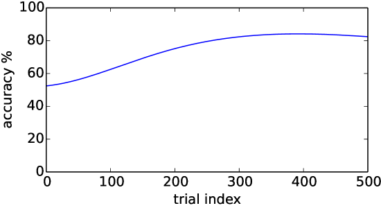
(a) Behavioral accuracy
(b) STFT-R slope time series	(c) MNE-R slope time series
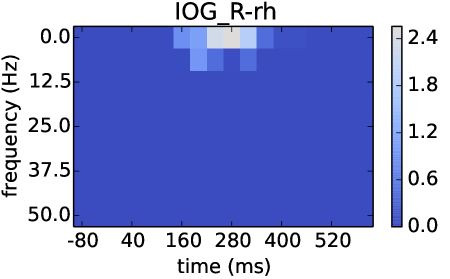
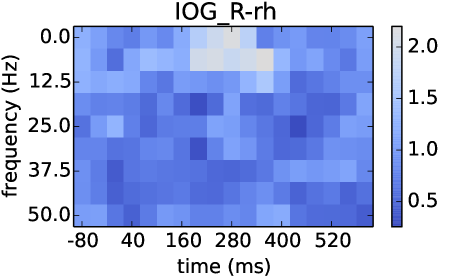
(d) STFT-R averaged absolute T	(e) MNE-R averaged absolute T

Figure 3: Face-learning experiment results for one participant. (a), Smoothed behavioral accuracy for Category 0. (b) and (c), Time series reconstructed from the STFT slope coefficients in trials with faces of Category 0 . Each curve denotes one source point. The shaded bands show 95% confidence intervals. (d,e) Averaged absolute Ts by STFT-R and MNE-R.

We report here results in one of the face selective regions, the right inferior occipital gyrus (labelled as IOG_R-rh), for one participant and one face category. This area is part of the “occipital face area” reported in the literature [Pitcher et al., 2011]. Since both STFT and the regression on the covariates are linear, we inversely transformed the slope coefficients of the STFT components to a time series for each source point, (denoted by “slope time series”), which showed the slope coefficient in the time domain (Fig. 3(b) and (c)). We observed that STFT-R produced smooth slope time series due to the sparse STFT representation (Fig. 3(b)), whereas MNE-R produced more noisy time series (Fig. 3(c)). We also show the previously defined averaged absolute Ts in the ROI, produced by STFT-R (Fig. 3(d)) and MNE-R (Fig. 3(e)) Compared with the dispersed pattern by MNE-R, STFT-R produced a more sparse pattern localized near $200\sim 300$ ms. We speculate that this pattern corresponds to the N250 component near 250 ms, which is related to familiarity of faces [Tanaka et al., 2006].

4 Discussion

To estimate learning effects in MEG, we introduced a source localization model (STFT-R), in which we embedded regression of STFT components of source signals on covariates, and exploited a hierarchical $L_{21}$ penalty to induce structured sparsity and emphasize regions of interest. We derived the FISTA algorithm and an active-set strategy to solve STFT-R. In reconstructing the ROI source signals from simulated data, STFT-R achieved smaller errors than a two-step method using MNE, and in a human learning experiment, STFT-R yielded more sparse and thus more interpretable results in identifying what time-frequency components of the ROI signals were correlated with learning. In future work, the STFT-R framework can also be used to regress MEG signals on high-dimensional features of stimuli, where the sparsity-inducing property will be able to select important features relevant to complex cognitive processes.
One limitation of STFT-R is its sparse representation of the non-ROI source points. In our simulation, all of the source points outside the four regions had zero signals, and it was reasonable to represent the two irrelevant regions as sparse source points. However, further simulations are needed to test how well STFT-R behaves when the true signals of the non-ROI source points are more dispersed. It is also interesting to develop a one-step regression model based on Bayesian source localization methods [Henson et al., 2011, Mattout et al., 2006], where we can relax the hard sparse constraints but still regularize the problem according to prior knowledge.

Appendix 1

Short-time Fourier transform (STFT) Our approach builds on the STFT implemented by Gramfort et al. in [Gramfort et al., 2013]. Given a time series $\bm{U}=\{U(t),t=1,\cdots,T\}$, a time step $\tau_{0}$ and a window size $T_{0}$, we define the STFT as

$$\Phi(\{U(t)\},\tau,\omega_{h})=\sum_{t=1}^{T}U(t)K(t-\tau)e^{(-i\omega_{h})}$$ (6)

for $\omega_{h}=2\pi h/T_{0},h=0,1,\cdots,T_{0}/2$ and $\tau=\tau_{0},2\tau_{0},\cdots n_{0}\tau_{0}$, where $K(t-\tau)$ is a window function centered at $\tau$, and $n_{0}=T/\tau_{0}$. We concatenate STFT components at different time points and frequencies into a single vector in $\bm{V}\in\mathbb{C}^{s}$, where $s=(T_{0}/2+1)\times n_{0}$. Following notations in [Gramfort et al., 2013], we also call the $K(t-\tau)e^{(-i\omega_{h})}$ terms STFT dictionary functions, and use a matrix’s Hermitian transpose $\bm{\Phi^{H}}$ to denote them, i.e. $(\bm{U}^{T})_{1\times T}=({\bm{V}}^{T})_{1\times s}(\bm{\Phi^{H}})_{s\times T}$.

Appendix 2

The Karush-Kuhn-Tucker conditions Here we derive the Karush-Kuhn-Tucker (KKT) conditions for the hierarchical $L_{21}$ problem. Since the term $f(\bm{z})=\frac{1}{2}\sum_{r=1}^{q}||\bm{M}^{(r)}-\bm{G}(\sum_{k=1}^{p}X_{k}^{(r)}\bm{Z}_{k})\bm{\Phi^{H}}||_{F}^{2}$ is essentially a sum of squared error of a linear problem, we can re-write it as $f(\bm{z})=\frac{1}{2}||\bm{b}-\bm{A}\bm{z}||^{2}$, where $\bm{z}$ again is a vector concatenated by entries in $\bm{Z}$, $\bm{b}$ is a vector concatenated by $\bm{M}^{(1)},\cdots,\bm{M}^{(q)}$, and $\bm{A}$ is a linear operator, such that $\bm{A}\bm{z}$ is the concatenated $\bm{G}(\sum_{k=1}^{p}X_{k}^{(r)}\bm{Z}_{k})\bm{\Phi^{H}},r=1,\cdots,q$. Note that although $\bm{z}$ is a complex vector, we can further reduce the problem into a real-valued problem by rearranging the real and imaginary parts of $\bm{z}$ and $\bm{A}$. Here for simplicity, we only derive the KKT conditions for the real case. Again we use $\{g_{1},\cdots,g_{h},\cdots,g_{N}\}$ to denote our ordered hierarchical group set, and $\lambda_{h}$ to denote the corresponding penalty for group $g_{h}$. We also define diagonal matrices $\bm{D}_{h}$ such that

$$\bm{D}_{h}(l,l)=\left\{\begin{array}[]{l l}1&\text{ if }l\in g_{h}\\ 0&\text{ otherwise }\end{array}\right.\forall h$$

therefore, the non-zero elements of $\bm{D}_{h}\bm{z}$ is equal to $\bm{z}|_{g_{h}}$. With the simplified notation, we re-cast the original problem into a standard formulation:

$$\min_{\bm{z}}(\frac{1}{2}\|\bm{b}-\bm{A}\bm{z}\|^{2}_{2}+\sum_{h}\lambda_{h}\|\bm{D}_{h}\bm{z}\|_{2})$$ (7)

To better describe the KKT conditions, we introduce some auxiliary variables, $\bm{u}=\bm{A}\bm{z},\bm{v}_{h}=\bm{D}_{h}\bm{z}$. Then (7) is equivalent to

$$\min_{\bm{z},\bm{u},\bm{v}_{h}} (\frac{1}{2}\|\bm{b}-\bm{u}\|^{2}_{2}+\sum_{h}\lambda_{h}\|\bm{v}_{h}\|_{2})$$

such that $$\bm{u}=\bm{A}\bm{z},\quad\bm{v}_{h}=\bm{D}_{h}\bm{z},\forall h$$

The corresponding Lagrange function is

$$L(\bm{z},\bm{u},\bm{v}_{h},\bm{\mu},\bm{\xi}_{h})=\frac{1}{2}\|\bm{b}-\bm{u}\|^{2}_{2}+\sum_{h}\lambda_{h}\|\bm{v}_{h}\|_{2}+\bm{\mu}^{T}(\bm{A}\bm{z}-\bm{u})+\sum_{h}\bm{\xi}_{h}^{T}(\bm{D}_{h}\bm{z}-\bm{v}_{h})$$

where $\bm{\mu}$ and $\bm{\xi}_{h}$’s are Lagrange multipliers. At the optimum, the following KKT conditions hold

$$\frac{\partial{L}}{\partial{\bm{u}}} =\bm{u}-\bm{b}-\bm{\mu}=0$$ (8)

$$\frac{\partial{L}}{\partial{\bm{z}}} =\bm{A}^{T}\bm{\mu}+\sum_{h}\bm{D}_{h}\bm{\xi}_{h}=0$$ (9)

$$\frac{\partial{L}}{\partial{\bm{v}_{h}}} =\lambda_{h}\partial{\|\bm{v}_{h}\|_{2}}-\bm{\xi}_{h}\ni 0,\forall h$$ (10)

where $\partial{\|\cdot\|_{2}}$ is the subgradient of the $L_{2}$ norm. From (8) we have $\bm{\mu}=\bm{u}-\bm{b}$, then (9) becomes $\bm{A}^{T}(\bm{u}-\bm{b})+\sum_{h}\bm{D}_{h}\bm{\xi}_{h}=0$. Plugging $\bm{u}=\bm{Az}$ in, we can see that the first term $\bm{A}^{T}(\bm{u}-\bm{b})=\bm{A}^{T}(\bm{A}\bm{z}-\bm{b})$ is the gradient of $f(\bm{z})=\frac{1}{2}\|\bm{b}-\bm{A}\bm{z}\|_{2}^{2}$. For a solution $\bm{z}_{0}$, once we plug in $\bm{v}_{h}=\bm{D}_{h}\bm{z}_{0}$, the KKT conditions become

$$\nabla f(\bm{z})_{\bm{z}=\bm{z}_{0}}+\sum_{h}\bm{D}_{h}\bm{\xi}_{h}=0$$ (11)

$$\lambda_{h}\partial{\|\bm{D}_{h}\bm{z}_{0}\|_{2}}-\bm{\xi}_{h}\ni 0,\forall h$$ (12)

In (12), we have the following according to the definition of subgradients

$$\bm{\xi}_{h}=\lambda_{h}\frac{\bm{D}_{h}\bm{z}_{0}}{\|\bm{D}_{h}\bm{z}_{0}\|_{2}}\text{ if }\|\bm{D}_{h}\bm{z}_{0}\|_{2}>0$$

$$\|\bm{\xi}_{h}\|_{2}\leq\lambda_{h}\text{ if }\|\bm{D}_{h}\bm{z}_{0}\|_{2}=0$$

Therefore we can determine whether (11) and (12) hold by solving the following problem.

$$\min_{\bm{\xi}_{h}} \frac{1}{2}\|\nabla f(\bm{z})_{\bm{z}=\bm{z}_{0}}+\sum_{h}\bm{D}_{h}\bm{\xi}_{h}\|_{2}^{2}$$

subject to $$\bm{\xi}_{h}=\lambda_{h}\frac{\bm{D}_{h}\bm{z}_{0}}{\|\bm{D}_{h}\bm{z}_{0}\|_{2}}\text{ if }\|\bm{D}_{h}\bm{z}_{0}\|_{2}>0$$

$$\|\bm{\xi}_{h}\|_{2}\leq\lambda_{h}\text{ if }\|\bm{D}_{h}\bm{z}_{0}\|_{2}=0$$

which is a standard group lasso problem with no overlap. We can use coordinate-descent to solve it. We define $\frac{1}{2}\|\nabla f(\bm{z})_{\bm{z}=\bm{z}_{0}}+\sum_{h}\bm{D}_{h}\bm{\xi}_{h}\|_{2}^{2}$ at the optimum as a measure of violation of the KKT conditions.
Let $f_{J}$ be the function $f$ constrained on a set $J$. Because the gradient of $f$ is linear, if $\bm{z_{0}}$ only has non-zero entries in $J$, then the entries of $\nabla f(\bm{z})$ in $J$ are equal to $\nabla f_{J}(\bm{z}|_{J})$ at $\bm{z}=\bm{z}_{0}$. In addition, $\bm{\xi}_{h}$’s are separate for each group. Therefore if $\bm{z}_{0}$ is an optimal solution to the problem constrained on $J$, then the KKT conditions are already met for entries in $J$ (i.e. $\left(\nabla f(\bm{z})_{\bm{z}=\bm{z}_{0}}+\sum_{h}\bm{D}_{h}\bm{\xi}_{h}\right)|_{J}=0$); for $g_{h}\not\subset J$, we use ( $\frac{1}{2}\|\left(\nabla f(\bm{z})_{\bm{z}=\bm{z}_{0}}+\sum_{h}\bm{D}_{h}\bm{\xi}_{h}\right)|_{g_{h}}\|^{2}$) at the optimum as a measurement of how much the elements in group $g_{h}$ violate the KKT conditions, which is a criterion when we greedily add groups (see Algorithm 2).

References

- [Bach et al., 2011] Bach, F., Jenatton, R., Mairal, J., and Obozinski, G. (2011). Optimization with sparsity-inducing penalties. CoRR, abs/1108.0775.
- [Beck and Teboulle, 2009] Beck, A. and Teboulle, M. (2009). A fast iterative shrinkage-thresholding algorithm for linear inverse problems. SIAM Journal on Imaging Sciences, 2(1):183–202.
- [Dale et al., 2000] Dale, A. M., Liu, A. K., Fischl, B. R., Buckner, R. L., Belliveau, J. W., Lewine, J. D., and Halgren, E. (2000). Dynamic statistical parametric mapping: combining fmri and meg for high-resolution imaging of cortical activity. Neuron, 26(1):55–67.
- [Galka et al., 2004] Galka, A., Ozaki, O. Y. T., Biscay, R., and Valdes-Sosa, P. (2004). A solution to the dynamical inverse problem of eeg generation using spatiotemporal kalman filtering. NeuroImage, 23:435–453.
- [Gauthier et al., 2000] Gauthier, I., Tarr, M. J., Moylan, J., Skudlarski, P., Gore, J. C., and Anderson, A. W. (2000). The fusiform “face area” is part of a network that processes faces at the individual level. Journal of cognitive neuroscience, 12(3):495–504.
- [Gramfort et al., 2014] Gramfort, A., Luessi, M., Larson, E., Engemann, D. A., Strohmeier, D., Brodbeck, C., Parkkonen, L., and Hämäläinen, M. S. (2014). Mne software for processing meg and eeg data. NeuroImage, 86(0):446 – 460.
- [Gramfort et al., 2013] Gramfort, A., Strohmeier, D., Haueisen, J., Hamalainen, M., and Kowalski, M. (2013). Time-frequency mixed-norm estimates: Sparse m/eeg imaging with non-stationary source activations. NeuroImage, 70(0):410 – 422.
- [Hamalainen et al., 1993] Hamalainen, M., Hari, R., Ilmoniemi, R. J., Knuutila, J., and Lounasmaa, O. V. (1993). Magnetoencephalography–theory, instrumentation, to noninvasive studies of the working human brain. Reviews of Modern Physics, 65:414–487.
- [Hamalainen and Ilmoniemi, 1994] Hamalainen, M. and Ilmoniemi, R. (1994). Interpreting magnetic fields of the brain: minimum norm estimates. Med. Biol. Eng. Comput., 32:35–42.
- [Henson et al., 2011] Henson, R. N., Wakeman, D. G., Litvak, V., and Friston, K. J. (2011). A parametric empirical bayesian framework for the eeg/meg inverse problem: generative models for multi-subject and multi-modal integration. Frontiers in human neuroscience, 5.
- [Jenatton et al., 2011] Jenatton, R., Mairal, J., Obozinski, G., and Bach, F. (2011). Proximal methods for hierarchical space coding. J. Mach. Learn. Res, 12:2297–2334.
- [Kanwisher et al., 1997] Kanwisher, N., McDermott, J., and Chun, M. M. (1997). The fusiform face area: a module in human extrastriate cortex specialized for face perception. The Journal of Neuroscience, 17(11):4302–4311.
- [Lamus et al., 2012] Lamus, C., Hamalainen, M. S., Temereanca, S., Brown, E. N., and Purdon, P. L. (2012). A spatiotemporal dynamic distributed solution to the meg inverse problem. NeuroImage, 63:894–909.
- [Mattout et al., 2006] Mattout, J., Phillips, C., Penny, W. D., Rugg, M. D., and Friston, K. J. (2006). Meg source localization under multiple constraints: an extended bayesian framework. NeuroImage, 30(3):753–767.
- [Pascual-Marqui, 2002] Pascual-Marqui, R. (2002). Standardized low resolution brain electromagnetic tomography (sloreta): technical details. Methods Find. Exp. Clin. Pharmacol., 24:5–12.
- [Pitcher et al., 2011] Pitcher, D., Walsh, V., and Duchaine, B. (2011). The role of the occipital face area in the cortical face perception network. Experimental Brain Research, 209(4):481–493.
- [Stine, 1985] Stine, R. A. (1985). Bootstrp prediction intervals for regression. Journal of the American Statistical Association, 80:1026–1031.
- [Tanaka et al., 2006] Tanaka, J. W., Curran, T., Porterfield, A. L., and Collins, D. (2006). Activation of preexisting and acquired face representations: the n250 event-related potential as an index of face familiarity. Journal of Cognitive Neuroscience, 18(9):1488–1497.
- [Xu, 2013] Xu, Y. (2013). Cortical spatiotemporal plasticity in visual category learning (doctoral dissertation).