Single Molecule Spectroscopy of Monomeric LHCII: Experiment and Theory

Abstract

We derive approximate equations of motion for excited state dynamics of a multilevel open quantum system weakly interacting with light to describe fluorescence detected single molecule spectra. Based on the Frenkel exciton theory, we construct a model for the chlorophyll part of the LHCII complex of higher plants and its interaction with previously proposed excitation quencher in the form of the lutein molecule Lut 1. The resulting description is valid over a broad range of timescales relevant for single molecule spectroscopy, i.e. from ps to minutes. Validity of these equations is demonstrated by comparing simulations of ensemble and single-molecule spectra of monomeric LHCII with experiments. Using a conformational change of the LHCII protein as a switching mechanism, the intensity and spectral time traces of individual LHCII complexes are simulated, and the experimental statistical distributions are reproduced. Based on our model, it is shown that with reasonable assumptions about its interaction with chlorophylls, Lut 1 can act as an efficient fluorescence quencher in LHCII.

Introduction

Photosynthesis, arguably the most important photo-induced process on Earth, converts the energy of light into its chemically/biologically useful form. It is often argued that this conversion is remarkably efficient. However, it has to be distinguished between the quantum efficiency, reaching almost unityBlankenshipBook ; Wraight1974 , and light-to-chemical energy efficiency, which is significantly lower, in the order of several percentBlankenship2011 . This is given by an evolutionary pressure on the development of a robust photosynthetic machinery optimized for survival rather than energy conversion efficiency. Energy relaxation processes are integral part of the photosynthetic function as they enable the energy transfer to proceed unidirectionally VanAmerongen2000 , and provide protection of the photosynthetic apparatus against harmful over-excitation. The photosynthetic machinery of plants has developed a complex hierarchy of self-regulatory mechanisms to avoid excess excitation or (when unavoidable) to dissipate it into heat Ruban2012 . Starting from processes controlled on the macroscopic level (e. g. orientation of leaves), over spontaneous microscopic (cellular) events such as chloroplast movements, to truly nano- and sub-nanoscopic mechanisms such as reorganization of antenna complexes and direct regulation of energy transfer on the level of small groups of interacting chromophores, plants actively react to changing illumination conditions. The sub-nanoscopic processes, which are the focus of the present study, operate in response to the increase of $\Delta{\rm pH}$ across the thylakoid membrane. Such an increase is an indicator of high illumination. Nowadays it is generally accepted that carotenoids are involved in these energy dissipation processes. The precise molecular mechanism is, however, still subject of discussionHolt2005 ; Ruban2007 ; Avenson2008 ; Bode2009 ; Berera2010 ; Muller2010 ; Fuciman2012 ; Staleva2015 . It is likely that different mechanisms evolved in different classes of organisms and/or that several mechanisms operate at once.

Most of our current knowledge about the early processes of photosynthesis was obtained by ultrafast spectroscopy. While conventional bulk spectroscopies are extremely useful in following ultrafast photo-induced events in photosynthesis, whenever structural inhomogeneity of the sample is involved, the information obtained from these spectroscopies becomes obscured by an inevitable ensemble averaging. Some well established spectroscopic methods, such as hole-burning Haarer1990 ; Johnson1989 ; Creemers1999 , and some modern multidimensional methods, such as coherent two-dimensional spectroscopy Jonas2003 , provide certain access to the homogeneous properties. Information on the behaviour of individual molecules has been, however, available only since the advent of single-molecule spectroscopy (SMS) Moerner1989 .

The system studied in this work, the light harvesting complex II (LHCII) of higher plants, is the plants’ major light-harvesting antenna containing almost half of all the chlorophyll in the chloroplast. Correspondingly, most of the light absorption and subsequent energy transfer processes in plants and algae occur in this complex. The LHCII antenna occurs naturally in a trimeric form and its main function is to deliver excitation energy to the nearby photosystem II (PSII). Given the major role of LHCII in light-harvesting and energy transfer, it is not surprising that it is also implicated in participating in regulated energy dissipation, the so-called non-photochemical quenching (NPQ) Ruban2007 ; Bode2009 ; Schlau-Cohen2015 . The crystal structure of the complex Liu2004 enables us efficient theoretical modeling of the complex’s spectroscopic properties using its chromophores (chlorophylls (Chl) and carotenoids) as the model units. The model parameters such as electronic coupling are greatly constrained by the known mutual orientation and distances. Existence of a large body of previous measurements together with theoretical attempts to fit this whole body of data to a single model Novoderezhkin2004 ; Novoderezhkin2005a ; Novoderezhkin2011 gives a great confidence in extending the modeling towards single molecular experiments.

In recent years, single-molecule spectroscopy (SMS) experiments on several photosynthetic antenna complexes including the LHCII were performed. Fluorescence spectral peak distributions Kruger2010 , spectral diffusion Tietz2001 , fluorescence intensity distributions Kruger2011 ; Kruger2012 and time traces Kruger2011a were obtained from these measurements. In many cases also fluorescence intermittency (blinking) was observed, and it was conjectured that in the case of LHCII the process behind the fluorescence intermittency plays a role in NPQ Kruger2011 .

As far as the theory of the SMS of LHCII is concerned, the ensemble-averaged spectra and also the peak distributions of LHCII trimers can be successfully explained by the disordered excitonic model Kruger2010 . In general, the excitonic model was successfully applied in the past on fs to ps timescale, and it represents an indispensable tool in analyzing ultrafast spectroscopic experiments on molecular aggregates and in particular on photosynthetic antennaeVanAmerongen2000 . Its application to longer time scales of seconds and minutes is conditioned by the assumption of a certain separation of time-scales. Over the course of the excitation-emission cycle (nanoseconds), individual chromophores of a complex are assumed to be found in fixed spatial arrangements and experiencing an environment described by a fixed set of parameters. The emission spectrum of a complex in such a fixed spatial arrangement is predicted by the excitonic model which gives the population distribution of the excited state manifold and the probability of emission at the corresponding transition frequencies. The spectrum of exciting light matters only to the extent to which the excited states reached at a given excitation wavelength are connected to the final state by some relaxation pathways. Once the pathways are available, the final state is given irrespective of the initial state after absorption of light. Because only the final distribution of excited state population matters, the changes (switches) of the spatial arrangement or environmental conditions occurring on the sub-nanosecond time scale are only observed as sudden changes (with respect to the nanosecond fluorescence time scale) of the fluorescence spectra. Despite the fact that the experiment we analyze in this work does not provide more insight into the sub-nanosecond dynamics of individual complexes than previous works, we nevertheless formulate the theory consistently in such a way that it enables the description of such processes. This is done in order to highlight the existence of a less studied type of processes on an intermediate time scale and to stress the need to search for experimental techniques which can cover the range of timescales from femtoseconds to nanoseconds in single molecular spectroscopy. We thus provide theoretical techniques to treat these future experiments. We have recently reported a progress towards measuring processes on the order of hundreds of femtoseconds in single light-harvesting complexes Maly2015 .

The paper is organized as follows: In Section I.1 we first discuss the Frenkel exciton model as a basis for the formulation of equations of motion for the populations of the excited states of chromophore aggregates with strong interchromophore couplings. Then, in Section I.2, we introduce equations of motion for excitonic populations valid over a broad (from ps to min) timescale range. We discuss their generality and the range of validity. It is argued that these equations provide an ideal means for the description of the SMS experiments. In Section I.3 the results of Section I.2 are applied to LHCII photosynthetic antenna complexes. All results are compared to the experiment. It is shown that our equations give correct fluorescence spectrum and peak statistics, i. e. appropriate steady-state population, under typical SMS experiment condition. Then we model the intensity traces, while the switching behaviour is included by incorporating one particular previously proposed NPQ mechanism, namely energy transfer to lutein Lut 1. The switching between on and off states is controlled by a 2-level model, where the switching causes a change of the Chl a612 - Lut 1 coupling. It is shown that using realistic parameters we are able to reproduce the experimental results. The details of our energy relaxation theory and of the stochastic model of switching are given in Supporting Information (SI).

I Results

I.1 Frenkel-Exciton model

In the usual SMS experiments, time-resolved (on the times scale of 10 ms to s) fluorescence of the studied molecules is observed. If the excited state life time of the studied chromophores is sufficiently long (nanoseconds in the case of chlorophylls studied here), the expected fluorescence spectra can be calculated from the steady state, quasi-equilibriated populations of the excited electronic eigenstates of the molecular system, assuming canonical equilibrium. Depending on the strengths of the chromophore-chromophore resonance interaction and the system-bath couplings, the eigenstates can be approximated either by the excited eigenstates of the electronic subsystem or the excited state of the individual chromophores forming the aggregate. In the present paper, we treat both cases within one formalism provided by the framework of the Frenkel exciton model.

The Frenkel exciton model provides an excellent tool for the treatment of pigment-protein complexes on femto- and pico-second time scales VanAmerongen2000 . The basic notion of the Frenkel exciton model is the one of localized excited states of the chromophores. These states have negligible wavefunction overlap with neighboring excited states, and they can therefore be assumed orthogonal to each other, forming a suitable basis for the aggregate Hilbert space. In the treatment of linear absorption and fluorescence experiments, only singly excited collective states of the molecular aggregate have to be included. The localized excited states can thus be denoted as $|i\rangle=|e_{i}\rangle\prod_{n\neq i}|g_{n}\rangle,$where $|g_{i}\rangle$ and $|e_{i}\rangle$ are the electronic ground and excited states of the chromophore denoted by index $i$, respectively. The states $|i\rangle$ form a complete Hilbert subspace for the case that exactly one molecule of the aggregate is excited. The molecular system Hamiltonian, $H_{S}$, is however rarely diagonal in the basis of the states $|i\rangle$ and resonance couplings $J_{ij}$ between excited electronic states $|i\rangle$ and $|j\rangle$ occur in all situations interesting for light-harvesting. In the absence of a protein environment, the light would resonantly excite eigenstates of the system Hamiltonian. In all realistic cases, the interaction of the system with its environment co-determines the excitation frequencies, and prescribes thus a “preferred basis” of electronic states in which it is the most advantageous to formulate the energy transfer theory.

In the case of the resonance interaction $J_{ij}$ exceeding the typical reorganization energy $\lambda$ of the protein bath of the chromophores $i$ and $j$, ($J_{ij}>\lambda)$, we include $J_{ij}$ explicitly into the system Hamiltonian. The Hamiltonian is diagonalized to obtain electronic eigenstates, and the effect of the protein bath is included via perturbation theory yielding a Redfield type relaxation tensor. In the opposite case $(J_{ij}<\lambda)$ we neglect the resonance coupling in the system Hamiltonian, and its effects are included perturbatively yielding Förster type energy transfer rates between localized excited states VanAmerongen2000 ; MayKuhn ; MancalBook .

I.2 Excited State Dynamics across Time-Scales

Let us first focus on deriving a closed set of equations for the excited state populations. Extensive work was done in the last years on developing methods to accurately describe the system dynamics following an ultrafast excitation by external light. The traditional Redfield and Förster approaches were superseded by more accurate (exact in some cases) methods, such as HEOM Ishizaki2009 ; Hein2012 ; Wilkins2015 , TEDOPA Prior2010 and other methods Shi2004 ; Stockburger2002 ; Xu2005 ; Huo2010 ; Schroter2014 . These methods bring unprecedented accuracy at an increased numerical cost. It seems, however, that for analyzing many of the recent experiments, it is still possible to rely on the traditional tools, as they capture the physics of the problem (and often even the quantitative aspects of the problem) very well Wilkins2015 .

Commonly, equations of motion for some relevant degrees of freedom (DOF), electronic states in our case, are derived by reducing the Liouville - von Neumann equation for the total density matrix to an equation for the so-called reduced density matrix (RDM). These equations describe time evolution of a molecular system for a fixed configuration of the protein environment (assuming fast fluctuations around this fixed configuration), and they are therefore suitable for the description of ultrafast laser experiments. However, on the timescale relevant in SMS (up to tens of seconds), usage of these equations is actually not appropriate. First of all, some transient effect at the short times affect even the long time properties of the system and the steady state population dynamics, and second, slow changes in the protein environment can entirely change the energy landscape including the case that one has to change the theoretical limit (localized states, delocalized states) in which one works. The latter case is especially difficult to treat and requires to go beyond the traditional master equation approaches which we apply here. In this work we therefore concentrate on the extension of the validity of the master equation approach towards long times under the assumption that the dependence of the Hamiltonian of the system on time is negligible within one absorption emission time scale (nanoseconds). As for the transient effects at short time, when dealing with fast dephasing of optical coherences, short time transient effects are responsible for the absorption lineshape. This aspect of the transient effects will be taken into account in full.

Spontaneous emission of photons by chlorophylls occurs with a nanosecond life-time. Another class of transient effects, namely dynamic electronic coherence due to excitation by light, is therefore also unimportant and its treatment can be avoided. We therefore derive approximative equations for the populations dynamics only, with the validity in the range from picoseconds to tens of seconds.

Initially, our Hamiltonian consists of the system, bath and system-bath interaction terms, and we formally assume some total density matrix $W(t)$ which follows the Liouville–von Neumann equation. There are several methods how to arrive to a master equation (in a convolution-less form) RDM $\rho(t)=Tr_{B}W(t)$ Fain2000 ; MancalBook . In general, such equation reads:

$$\frac{\partial}{\partial t}\rho(t)=-\frac{i}{\hbar}[H(t,t_{0}),\rho(t)]-{\cal R}(t,t_{0})\rho(t),$$ (1)

$$H(t,t_{0})=H_{S}(t_{0})-\mu E(t).$$ (2)

The total Hamiltonian $H$ consists of the bath renormalized system Hamiltonian $H_{S}(t_{0})$ and the system-light interaction, which is (in the dipole approximation) given by the dipole moment operator $\mu$ and electric field $E(t)$. The bath is completely eliminated in the reduced description, and its effects are represented by the relaxation tensor ${\cal R}(t,t_{0})$. It is important to note that in Eq. (1), the relaxation tensor ${\cal R}(t,t_{0})$ explicitly depends on some initial time $t_{0}$, in which the initial condition for the propagation is set, or more precisely, the relaxation tensor depends on the quantity $t-t_{0}$. An exact relaxation tensor would also depend on $E(t)$. In general, the choice of $t_{0}$ is arbitrary, and we should choose it such that the temporal profile of the excitation field is non-zero for $t>t_{0}$ only. However, in most practical theoretical approaches, the evolution of the bath due to excitation of the system is reflected in the relaxation tensor ${\cal R}(t,t_{0})$ by the bath correlation function, which decays rather quickly. By choosing $t_{0}$ sufficiently small, we could always make such a relaxation tensor constant. This is obviously an artifact of the approximations used. For a smooth envelope of the external field changing on the same or slower timescale than the correlation function of the bath, there is no good choice of $t_{0}$. The relaxation tensor always becomes constant too early. Luckily, as we will see below, we do not need to account for the external field $E(t)$ beyond first order perturbation theory, and in this regime, there is a natural choice of time $t_{0}$ which enables us to correctly account for the transient time dependence of the relaxation tensor even for a steady state externally driven by light. It is important to note, that the relaxation tensor ${\cal R}(t,t_{0})$ is completely abstract up to now. It can represent some exact relaxation superoperator, or a result of perturbation theory with respect to some parameters, such as the Redfield or Förster tensors.

Let us now formulate the equations of motion for the excited state evolution in the linear regime of the system’s interaction with the electric field. The validity of the linear regime has been discussed e.g. in Refs. Jiang1991 ; Mancal2010 ; Brumer2012a ; Chenu2014 , and it is the same as the validity of the third order response theory for non-linear laser spectroscopy. We will also use the secular approximation (equations of motion for populations $\rho_{ii}$ and coherences $\rho_{ij}$, $i\neq j$ are assumed independent), although this we do only to simplify the resulting equations. Secular approximation could be avoided if one so wishes, at the cost of treating the full DM. We write explicitly the elements of the RDM of Eq. (1) in which we keep the double time dependence of the Hamiltonian and the relaxation tensor. We get the following set of coupled equations:

$$\frac{\partial\rho_{ii}(t)}{\partial t}=\sum_{j}k_{ij}(t,t_{0})\rho_{jj}(t)-\Gamma_{i}(t,t_{0})\rho_{ii}(t)+(i\mu_{i0}\rho_{0i}(t)E(t)+c.c.),$$ (3)

$$\frac{\partial\rho_{i0}(t)}{\partial t}=-i\omega_{i0}(t_{0})\rho_{i0}-\gamma_{i}(t,t_{0})\rho_{i0}(t)+i\mu_{i0}(\rho_{00}-\rho_{ii}(t))E(t).$$ (4)

Here, the $k_{ij}(t,t_{0})\equiv{\cal R}_{iijj}(t,t_{0})$ are transfer rates between populations (from $j$ to $i$), $\Gamma_{i}(t,t_{0})\equiv\tilde{\Gamma}_{i}+{\cal R}_{iiii}(t,t_{0})$ is the population relaxation rate of the state $i$, including the rate of radiative depopulation $\tilde{\Gamma}_{i}$ (we assume it is constant), and $\gamma_{i}(t,t_{0})\equiv{\cal R}_{i0i0}(t,t_{0})$ is the optical coherence dephasing rate.

The equation of motion for the optical coherences, Eq. (4), can be solved by introducing the interaction picture using the evolution operator element ${\cal U}_{i0i0}(t,t^{\prime})$, and integrating Eq. (4) in the interaction picture. By returning back to the Schrödinger picture, we obtain the actual field-induced and field driven optical coherence element in the form:

$$\rho_{i0}(t)=i\int_{0}^{t-t_{0}}dt^{\prime}{\cal U}_{i0i0}(t,t-t^{\prime})\mu_{i0}[\rho_{00}(t-t^{\prime})-\rho_{ii}(t-t^{\prime})]E(t-t^{\prime}).$$ (5)

We can see that Eq. (5) is actually not a solution of Eq. (4). In solving Eq. (4) numerically, the dephasing rate would quickly become constant for $t\gg t_{0}$ and the transient effects for $t-t_{0}\approx 0$ would be lost completely. However, in Eq. (5) these effects are properly taken into account. The discrepancy between Eq. (4) and Eq. (5) is due to a different treatment of the bath. In a response function approach, of which the linearization of the full equations of motion with respect to the field is a variant, it is in general possible to account for the bath in a more consistent way than in master equations. In ordinary master equations, the bath is correctly described at $t_{0}$, and the description of its subsequent evolution after $t_{0}$ is extremely limited. An example of such limitation is discussed e.g. in Ref. Mancal2012 .

In most biological energy transferring systems, the pure dephasing is much faster (hundreds of fs) than the population relaxation (units and tens of ps). We can therefore assume that the populations remain constant during the integration in Eq. (5). Moreover, it is reasonable to set the upper limit of the integration in Eq. (5) to infinity by sending $t_{0}\rightarrow-\infty$. We can expect that the simultaneous action of pure dephasing and external driving by a field with a slowly varying envelop creates a steady state optical coherence. The dependence on $t_{0}$ in the upper limit of the integral describes a transient evolution of the optical coherence after switching on the interaction with the field. Now that the short time time-dependent nature of the dephasing rates is taken into account correctly, we can set $t_{0}\rightarrow-\infty$ and write:

$$\rho_{i0}(t)=i\int_{0}^{\infty}dt^{\prime}{\cal U}_{i0i0}(t,t-t^{\prime})E(t-t^{\prime})\mu_{i0}[(\rho_{00}(t)-\rho_{ii}(t)].$$ (6)

It is important to note that now $t$ is a global time which can run through the whole minutes long SMS experiment. The evolution operator changes on an ultrafast time scale, but this timescale is scanned in the integration over the variable $t^{\prime}$. The properties of the Hamiltonian $H_{S}(t)$ change on a very slow time scale (with respect to optical dephasing), and so does the evolution operator element ${\cal U}_{i0i0}(t,t-t^{\prime})$. Unlike the Eq. (4), which is valid for $t-t_{0}$ small, Eq. (6) is valid for all times.

The purpose of deriving Eq. (6) was to insert it eventually into Eq. (3). Also here we face the problem of transient time dependence of the rates. However, because populations change much more slowly, these effects are not as important as in the case of coherences. They can be, however, treated rigorously, even including bath memory effects between evolutions by Eq. (4) and Eq. (3), as we have shown elsewhere Olsina2012 . In this work, we will assume the energy transfer and relaxation rates not to depend on the difference $t-t_{0}$, although they may depend weakly on the time $t$, i. e. $k_{ij}(t,t_{0})=k_{ij}(t)$ and $\Gamma_{i}(t,t_{0})=\Gamma_{i}(t)$. We are ready now to insert Eq. (6) for optical coherences into the equation for populations, Eq. (3). We obtain

$$\frac{\partial P_{i}(t)}{\partial t}=\sum_{j}k_{ij}(t)P_{j}(t)-\Gamma_{i}(t)P_{i}(t)+|\mu_{i0}|^{2}(P_{0}(t)-P_{i}(t))\cdot 2{\rm Re}\int_{0}^{\infty}dt^{\prime}E(t)E(t-t^{\prime}){\cal U}_{i0i0}(t,t-t^{\prime}).$$ (7)

Here, we defined $P_{i}(t)=\rho_{ii}(t)$, and we used the fact that $\mu_{i0}$ and even ${\cal U}_{i0i0}(t,t^{\prime})$ are ordinary c-numbers.

In Eq. (7), the populations are driven by a second order field term. We have treated the field classically so far. If we did that quantum mechanically, we would now have to trace over the field DOF in order to obtain reduced equations of motion for the electronic state populations only. The term $E(t)E(t-t^{\prime})$ would thus be replaced by $\left\langle E(t)E(t-t^{\prime})\right\rangle$ which can be interpreted as a quantum mechanical expectation value. The latter expression has the form of two-time correlation function of the electric fields of the light and its Fourier transform is the power spectrum of the light Jiang1991 ; Brumer2012a ,

$$\left\langle E(t)E(t-\tau)\right\rangle=\int_{0}^{\infty}d\omega W(\omega)e^{i\omega\tau}.$$ (8)

Now, inserting Eq. (8) into Eq. (7), switching the order of integrations, and using the definition of absorption lineshape of the i-th excitonic transitions (see e.g. MukamelBook )

$$\chi_{i}(\omega;t)=|\mu_{i0}|^{2}\int_{0}^{\infty}dt^{\prime}e^{i\omega t^{\prime}}{\cal U}_{i0i0}(t,t-t^{\prime}),$$ (9)

we arrive at

$$\frac{\partial P_{i}(t)}{\partial t}=\sum_{j}k_{ij}(t)P_{j}(t)-\Gamma_{i}(t)P_{i}(t)+\left[P_{0}(t)-P_{i}(t)\right]\int d\omega W(\omega)\chi_{i}(\omega;t).$$ (10)

Our effort has yielded a closed set of equations for excitonic populations only. The population changes are given by the transfer rates between electronic levels, population quenching and a source terms expressed as an overlap of the excitonic spectra with the light spectrum. All quantities are in principle dependent on time, most importantly the excitonic absorption spectrum and all rates can weakly depend on time to simulate slow changes of the protein and chromophore configurations. Also the light spectrum can be considered time-dependent by generalizing the Wiener-Khintchine theorem for the instaneous power spectrum $W(\omega,t)$Page1952 ; Jiang1991 . The changes can be faster than the time resolution of the SMS experiment, but they have to be slower than the dephasing, or even energy transfer dynamics.

We should also note here that if we wish to stay strictly in the linear regime, the saturation term $(P_{0}-P_{i})$ in Eq. (10) should be very close to one. In fact, we can set it equal to one as a reasonable approximation with the same validity as the linear approximation for fields.

I.3 Spectroscopy of LHCII Complex

I.3.1 Excitonic Model for Bulk and Single Molecule Spectra

According to crystalographic studies, LHCII complex consists of three monomeric units, each containing 14 chlorophylls and for carotenoids: two luteins, neoxanthin and a carotenoid of the xanthophyll cycleLiu2004 . The experiments described in this section were performed on monomeric LHCII complexes. In accord with the experiment, we focus on one such a monomeric unit in our model. We treat the LHCII monomer as a strongly coupled systems of chromophores, weakly coupled to the bath and weakly interacting with light. Because only absorption and fluorescence are measured, we do not attempt to fit the site energies in our simulations from scratch, as the fitting of this limited set of experiments would not be unique. Instead, we take the pigment transition energies from Ref. Novoderezhkin2005a , where both LHCII trimers and monomers where treated. The coupling energies between the pigments were calculated in the dipole-dipole approximation, and the dipole orientations were taken from the crystal structure using an effective dipole strengths of 3.4 D for Chl b and 4.0 D for Chl a. The bath is described by means of a spectral density obtained by fluorescence line narrowing experiment (FLN) (see Ref. Novoderezhkin2004 ; Peterman1997 ). Excitonic absorption and fluorescence lineshapes are calculated by means of the second order cumulant expansion (see Ref. MukamelBook ), and the population transfer rates are calculated by the multilevel Redfield theory (see Ref. MayKuhn ). For comparison, we also calculated the rates by Modified Redfield theory, Ref.Novoderezhkin2004 , and we concluded that the results remain essentially the same. The population relaxation rates of chlorophylls were taken to be 3 ns in accord with the experiment Nordlund1981 . The equations of motion, Eq. (10), allow us to use light with any spectral composition. In the experiment described in this paper, we use spectrally narrow (laser) illumination at 630 nm. For details on the calculations see SI.

In Figs. 1A and 1B we present the calculated bulk absorption and fluorescence spectra of LHCII monomers at 5° C compared to experimental values taken from Kruger2010 . We note here that the bulk spectra of LHCII in monomeric and trimeric form are practically identical, see Fig. S1 in SI for comparison. In calculations, the spectra were averaged over a Gaussian disorder of site energies with full width at half maximum (FWHM) of 110 cm^-1. Although the blue Chl b shoulder is not perfectly reproduced, the agreement between measured and theoretical absorption is good in the region of our excitation, and the fluorescence (FL) spectrum shows a good agreement in general. We therefore conclude that our excitonic model captures correctly the features of the studied system that are the most relevant in the present study.

The FL spectrum in Fig. 1B is dominated by the lowest four excitons, which are the most populated ones. These excitons are formed by strongly coupled pigments Chl 610-611-612, Chl 602-603 and Chl 613-14 (see Ref. Liu2004 for nomenclature). This is in agreement with previous modeling results for the trimeric LHCII Novoderezhkin2005a .

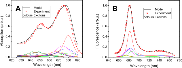
Figure 1: Bulk (A) Absorption and (B) Fluorescence spectrum of the Qy band of LHCII monomers. The points are experimental values taken from Ref. Kruger2010 , the lines are calculated by our exciton model. The coloured lines are individual excitonic contributions, the black line is the overal spectrum.

The calculated bulk spectra seem to be in a good agreement with the experiment. Our model also reproduces successfully the statistics from the SMS experiments. In Fig. 2A we present the FL spectral peak distribution compared to the experiment. We can see that the calculated distribution is a little broader than the experimental one, but the agreement is again reasonably good. The larger distribution width of the calculated spectra can be explained by a relatively long integration time in the experiment (1 s), during which the system samples several individual realizations of the disorder. In extreme cases the measured values get averaged towards the mean value. As a result the measured distribution is narrower. From our comparisons between experiments and calculations we conclude that the exciton model with Gaussian disorder not only reproduces the averaged absorption spectra and equilibriated populations of excitons (resulting in characteristic FL spectra), but also the individual realizations provided by this model are in a good agreement with the experiment.

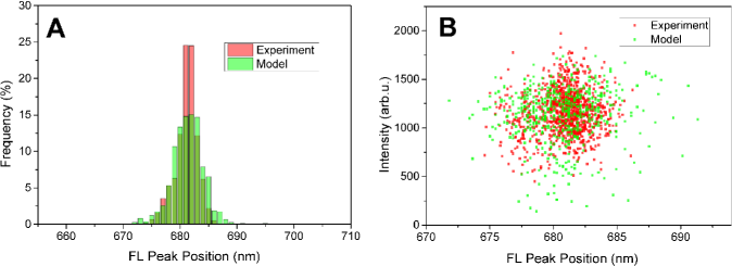
Figure 2: Experimental (red) and calculated (green) fluorescence peak distribution. (A) Peak position histogram, (B) FL peak position and intensity plot. Theoretical points are calculated as individual realizations of energetic disorder.

The next feature of the LHCII single molecular spectra that we need to address is the significant amount of blinking, i. e. reversible switching to the off state. Since the measured dwell times in the off state are in the range of seconds, which is significantly longer than the lifetime of any long-living species such as triplet states Schodel1998 , the off states must correspond to states with efficient excitation energy dissipation. Correspondingly, our model has to be extended by including some fluorescence quenching mechanism.

I.3.2 Lutein Lut 1 as a Fluorescence Quencher

One of the possible mechanism of FL quenching in LHCII, proposed by Ruban and coworkers Ruban2007 ; Duffy2013 , is an excitation energy transfer from the lowest chl a exciton states to a lutein molecule, Lut 1 (lut620), see Ref. Liu2004 for nomenclature). The Lut 1 molecule resides in the vicinity of the so-called terminal emitter group of chlorophylls, composed of Chls a610, 611 and 612, and it is supposed to be coupled mainly to Chl a612 Ruban2007 ; Duffy2013 . The S1 state of the Lut molecule is optically forbidden, and it has a short (10 ps) lifetime due to a decay through a non-radiative channel Polivka2002 . The transition energy from the S0$\rightarrow$S1 of Lut is in the vicinity of the transition to the Chl $Q_{Y}$ state. Due to its short excited state life-time, Lut could in principle act as an excitation (and fluorescence) quencher. Let us test this mechanism within our model to see if it can account for the observed blinking. The important parameters of the lutein in context of our model are its S1 state site energy relative to its groundstate and the coupling to chlorophylls, in particular to Chl a612.

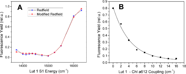
Figure 3: Role of Lut 1 parameters. Dependence of the fluorescence yield on (A) Lut 1 S1 energy and (B) Lut 1 - Chl a612 coupling. The energy dependence is calculated with Redfield (blue) and Modified Redfield (red) theory for comparison. The dependence on the coupling strength depicts calculated points (Redfield theory) fitted with exponential dependence. Already a realistically small coupling around $12\mbox{ cm}^{-1}$ leads to significant FL quenching.

In Fig. 3A we present the dependence of the relative FL quantum yield on the Lut energy for fixed value of the Lut-Chl coupling of 14 cm^-1. The energy dependence agrees well with the one obtained by Ruban Duffy2013 . The quenching is only efficient when the Lut energy is below one of the red chlorophylls (around 15100 cm^-1) and the plateau enables Lut to act as an efficient quencher even in disordered systems.

In Fig. 3B we show the dependency of the FL quantum yield on the Lut-Chl coupling for fixed Lut energy 14500 cm^-1. Due to large reorganization energy, 14500 cm^-1 corresponds to the zero-phonon line at 13900 cm^-1 and thus agrees with experimental observations Polivka2002 . From the coupling dependence of fluorescence in Fig. 3B we can conclude that weak coupling is sufficient for Lut 1 to act as a fluorescence quencher. Very importantly, even small changes in the Lut-Chl coupling can result in a big difference in the fluorescence intensity. Based on this analysis we decided to use lutein S1 site energy of 14500 cm^-1 in our simulations of blinking. We define the quenched state by the value of 12 cm^-1 for coupling of the Lut 1 to Chl 612 and the unquenched state by the zero coupling. Our model allows any type of time dependency of the Chl-Lut coupling to be used, and it could in principle accommodate input from structure based MD studies and quantum chemical treatment of the (Dexter type) coupling of the Chl $Q_{Y}$ and the Lut S1 states. However, a much rougher phenomenological model of the Chl-Lut coupling changes enables a better discussion of the feasibility of the proposed quenching mechanism than the parameter free ab initio calculations suffering from uncertainties in the structural information. Next we proceed to model the blinking statistics.

I.3.3 Model of the On-Off State Switching

As mentioned in the Introduction, the blinking statistics alone can be well described by a two-level model proposed by Valkunas et al. in Ref. Valkunas2012 . By random fluctuations, the protein samples its potential energy surface (PES) performing thus a random walk (RW). The model of Ref. Valkunas2012 assumes that there are two stable conformations of the protein corresponding to two minima of the protein PES. These are approximated by two harmonic potentials. The protein undergoes a RW in this potential, and at every step it has a certain probability to switch from its current PES to the other PES. In our treatment we use a discrete RW description, which enables us to follow individual trajectories of the proteins. For the details of the approach taken in this study and the differences from the original model by Valkunas et al., see SI and Refs. Valkunas2012 ; Chmeliov2013 .

To connect the two PES model to our particular Lut quenching model, we assume that the change of protein conformation somehow changes the Lut-Chl coupling. The Lut S1 state does not have a dipole moment, and the resonance coupling similar to those between allowed states does not occur here. The two different protein conformations responsible for the quenched/unquenched states would then result in two slightly different orientations/positions of the pigments, leading to different strengths of the coupling. This mechanism is in accord with recent quantum-chemical study by Duffy et al. Chmeliov2015b , where small configurational changes were found to lead to substantial changes in chl-car couplings. The switching between the PES is controlled by the RW model with diffusion parameters adjusted to fit the experimental dwell time distributions. The comparison between the calculated and experimentally determined dwell-times is presented in Figs. 4A and 4B, for the on and off times, respectively. The agreement is again fairly good letting us believe that our phenomenological model captures the most important features of the protein dynamics affecting the blinking behaviour.

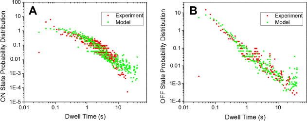
Figure 4: Experimental (red) and calculated (green) probability distribution of dwell times in the (A) ON and (B) OFF state, logarithmic scale. While the OFF state distribution follows a power law, the ON state distribution has an exponential tail at longer times.

I.3.4 Intensity traces

Finally, we can connect the two models described above and simulate the blinking behaviour. To this end we continuously model the fluorescence of the LHCII complexes, and output the intensity (and spectrum) every 10 ms corresponding to the experimental integration bins. Simultaneously, we let the protein do the RW on its PES, and we adjust the Chl/Lut coupling, when the protein switches between PES. To obtain more realistic traces, either the site energies or couplings can be slightly varied after every jump, resulting in different energy levels. Such a procedure, however, does not lead to qualitatively different conclusions and it can be in principle omitted. In the calculations presented here, we used Gaussian disorder with the FWHM of 0.3 cm^-1 for couplings and 1 cm^-1 for energies. For every realization of the disorder a 60 s trace is modelled. This is repeated for 200 realizations of the disorder, reflecting the experimental conditions. The resulting statistics are presented in Fig. 5.

Total dwell times in Fig. 5A represent the overall amount of time spent in a given intensity level. From this we can see the two-level character of the blinking and simultaneously also the presence of some intermediate levels, which result from particular disorder realizations. The dwell times are similar for the on and off states. Fig. 5B shows how often are the intensity levels visited per fixed amount of time. The modelled access frequency distribution is naturally very symmetrical, a direct result of the fact that in the model the complex switches only between the on and off state. The number of on/off states visited per minute therefore has to be the same. The experimentally analyzed intensity traces contain also jumps between levels within the on/off states in an amount which can be, to some extent, modified by adjusting the sensitivity of the level analysis. The presence of these intra-state jumps results in higher switching frequency and wider distribution in intensities, causing a moderate discrepancy between experiment and simulation. In order to include this kind of switching into the model, dynamic sampling of the disorder would have to be incorporated. Work in this direction will be presented elsewhere.

For the reasons stated above, the level access frequency distribution is not well suited for comparison of the model with the experiment. A more appropriate measure of the blinking would be the intensity-intensity correlation function defined as $h^{(2)}(\tau)=\nicefrac{{\left\langle I(\tau)I(0)\right\rangle}}{{\left\langle I(0)\right\rangle^{2}}}$. This quantity is well-known from single-molecule measurements, where it is often used to characterize the blinking behaviour SMSignalsBook . In Fig. 5C we present $h^{(2)}(\tau)$ obtained from 50 measured long enough traces, compared with the model. We can see that the agreement between experiment and theory is good, indicating that our model gives reasonable switching between the intensity levels. The shape of the correlation function is given by the dwell time statistics, see also Fig. 4. The initial fast drop implies the abundance of short blinking events. This results from the mechanism of the protein switching between its potential surfaces, where the short succesive blinking events are caused by the dynamics in the vicinity of the PES intersection.

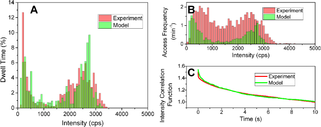
Figure 5: Experimental (red) and calcuated (green) intensity blinking statistics. (A) The percentage of time the complexes dwelled on respective intensity levels. The two-state structure of the low-intensity OFF states and higher intensity ON states is apparent. (B) How often per minute the complexes accessed the respective intensity levels. The experimental frequency is higher due to switching within the ON/OFF states. (C) The intensity correlation function.

Discussion

In Section I.2 of the Results we derived approximate equations of motion for populations evolution on the timescale of the SMS experiment. We have shown that the weak illumination regime, in which the SMS experiment is performed, allows for an effective source term description of the light-matter interaction in which short time transient effects arising in the photoinduced evolution of molecular systems can be consistently accommodated side by side with the slow evolution of the protein bath observed in SMS experiments. We demonstrated the validity and scope of application of our equations by simulating our single molecule experiment on LHCII monomers. Based on the recent research in elucidating the NPQ mechanism in LHCII and the connection between fluorescence quenching and energy dissipation we implemented energy transfer to Lut 1 as a blinking mechanism. Based on our calculations we were able to confirm the findings of Duffy et al. Duffy2013 and Chmeliov et al.Chmeliov2015b that, within a reasonable range of parameters, Lut 1 can indeed act as an efficient quencher. Since our model extends the previous treatment by including realistic excitation conditions and population transfer rates, it is remarkable, how similar our fluorescence quenching dependence on the Lut 1 energy is to the one in Ref. Duffy2013 . Moreover, we were able to confirm that Lut 1 acts as an efficient quencher also under AM1.5 illumination (data not shown since the dependence is very similar). At the same time we can see that the amount of quenching is very sensitive to the change of coupling of the Lut to the chlorophylls. Since the coupling itself is very sensitive to the distance and orientation between the pigments, it provides a possible link to the protein conformation change working as a switching mechanism as proposed in Ref. Valkunas2012 ; Chmeliov2015b . Indeed, when using the 2-level switching model to control the change of coupling, we are able to reproduce the experimentally obtained blinking statistics. Although far from being exclusive in any way, our argument strongly supports the notion of the protein acting as a conformational switch regulating the amount of quenching in the system.

The agreement between the theory and experiment also serves as a good demonstration of the scope of our equations. They provide a description for controlling the energy transfer in the system by modulating the parameters of the excitonic model. We are aware of the remaining phenomenological nature of our connection of the 2-level switching model with the excitonic model. Further improvements in the direction of introducing more parameters with a particular physical meaning, for example the relation to the actual PES shape, are needed and will be subject to further study. Also recent experimental observations indicate the presence of more relevant timescales in the intensity traces suggesting the inadequacy of a 2-level model with one reaction coordinate. Finally, although some connection between the fluorescence blinking and NPQ was already shown by Krüger et al. Kruger2011 , their exact relation is yet to be elucidated. The equations derived here are a suitable tool for these future investigations.

Methods

Sample preparation

Trimeric LHCII complexes of spinach were isolated from freshly prepared thylakoid membranes as described earlier VanRoon2000 . Monomeric complexes were obtained by incubating LHCII trimers with 1% (w/v) octyl glucoside and 10 $\mathrm{\mu g/mL}$ phospholipase A2 (Sigma) Nussberger1994 . Subsequent fast protein liquid chromatography (FPLC) ensured a homogeneous sample preparation. The ensemble fluorescence absorption and emission spectra were measured on a Lambda40 spectro-photometer (Perkin-Elmer) and a FluoroLog Tau-3 (Jobin Yvon), respectively. For SMS experiments, the sample was diluted down to a concentration of ~ 10 pM in a measuring buffer (20 mM Hepes, pH 8 and 0.03% (w/v) n-Dodecyl ${\textstyle\beta}$-D-maltoside) and then immobilized on a PLL (poly-L-Lysine, Sigma) coated cover glass. Addition of an oxygen scavenging mix of 750 $\mathrm{\mathrm{\mu g/ml}}$ Glucose Oxidase, 100 $\mathrm{\mu g/ml}$ Catalase and 7.5 $\mathrm{mg/ml}$ Glucose (all Sigma) to the closed sample chamber inhibited the formation of highly reactive singlet oxygen and improved the photostability of complexes.

Single-molecule detection

A confocal microscope was used to measure the fluorescence of single complexes at 5 ${}^{\circ}C$ as described previously Kruger2010 . The sample was excited at 630 nm utilizing a Ti:sapphire laser (Coherent MIRA 900F) with a pulse width of 200 fs and a repetition rate of 76 MHz coupled to a tunable optical parametric oscillator (Coherent MIRA OPO). Near-circular polarized light was obtained by utilizing a Berek polarization compensator (5540 New Focus). A fluorescence beam splitter (70:30, Thorlabs) allowed us to simultaneously measure the fluorescence spectrum via a CCD camera (Spec10:100BR, Roper Scientific) with an integration time of one second and the wavelength integrated fluorescence intensity via an avalanche diode (SPCM-AQR 16, Perkin Elmer) with a binning time of 10 milliseconds. The fluorescence of one complex was analyzed for either one minute or until it photo-bleached and a set of 200 complexes served as the basis for statistical analysis. The fluorescence peak distribution was obtained by fitting of a skewed Gaussian to the fluorescence spectrum as shown in Kruger et al. Kruger2010 and the blinking analysis was performed equivalently to the algorithm described elsewhere Kruger2011a .

Dynamics simulation

The equations of motion, Eq. (10), have quasi constant coefficients, and they can therefore be written in the form

$$\frac{\partial\mathbf{P}}{\partial t}=\mathbf{{\cal M}}\mathbf{P}+\mathbf{S},$$ (11)

where ${\cal M}$ is a matrix of relaxation and population transfer rates, and $\mathbf{S}$ are the source terms. Eq. (11) can be solved analytically:

$$\mathbf{P}(t)=\mathbf{{\cal M}}^{-1}(e^{\mathbf{{\cal M}}(t-t_{0})}-1)\mathbf{S}+e^{\mathbf{{\cal M}}(t-t_{0})}\mathbf{P}(t_{0}).$$ (12)

This expression enables us to find the populations at any time without the need to solve for all the previous times. If we aim at steady state, $t_{0}$ can be send to $-\infty$ and the populations then depend only parametrically on time $t$. The weak dependence of $\bm{{\rm S}}$ and ${\cal M}$ on $t$ makes it possible to explain changes in the populations of the emitting states of a molecular system due to slow changes of the protein environment and the structure of the molecular system.

Supplementary Information

Exciton model

The interaction of the pigments, i. e. the system, with the vibrations, i. e. its environment, is treated by second order perturbation theory. There the bath is completely described by its correlation function or, equivalently, in the frequency domain, by the spectral density of the bath vibrations. We use the spectral density from Ref. Novoderezhkin2004 . It is constructed from one overdamped oscillator representing the slow protein vibrations and 48 high-frequency intrapigment modes (for more context for the spectral density and excitonic model see Ref. MukamelBook ):

$$C^{\prime\prime}(\omega)=2\lambda_{0}\frac{\gamma_{0}\omega}{\omega^{2}+\gamma_{0}^{2}}+\sum_{i=1}^{48}2S_{j}\omega_{j}\frac{\omega_{j}^{2}\gamma_{j}\omega}{(\omega^{2}-\omega_{j}^{2})^{2}+\omega^{2}\gamma_{j}^{2}}.$$ (13)

The (temperature dependent) correlation function given by this spectral density is assumed to be uncorrelated between individual sites and differs only between Chl a and Chl b, while the difference is in the coupling strength $\nu_{n}=\nu_{a/b}$:

$$C_{n}(\omega)=\nu_{n}C(\omega)=\nu_{n}\left(1+\coth\left(\frac{\hbar\omega}{2k_{B}T}\right)\right)C^{\prime\prime}(\omega).$$ (14)

The time-dependent correlation function is then obtained by Fourier transform of (14). We use the same values of the spectral density parameters as in Ref. Novoderezhkin2004 . The difference between the vertical, Franck-Condon transition of the pigments, which are called site energies in this text, and their 0-0 transitions is given by the reorganization energy due to the interaction with the bath:

$$\lambda=\frac{1}{\pi}\int_{0}^{\infty}\frac{C^{\prime\prime}(\omega)}{\omega}.$$ (15)

Because the pigments are strongly coupled, the preferred basis of calculations is the excitonic basis in which the system Hamiltonian is diagonal with eigenvalues, exciton energies, $\omega_{i0}$. All quantities, including correlation functions $C(t)$, reorganization energies $\lambda$ and transition dipole moments $\mu$ have to be transformed into the excitonic basis:

$$C_{i}(t) =\sum_{n}|c_{i}^{n}|^{2}C_{n}(t),$$ (16)

$$\mu_{i0} =\sum_{n}c_{i}^{n}\mu_{n0},$$ (17)

$$\lambda_{i}=\sum_{n}|c_{i}^{n}|^{4}\nu_{n}\lambda.$$ (18)

The position of the zero phonon lines of the excitonic transitions is then

$$\omega_{i0}^{ZPL}=\omega_{i0}-\lambda_{i}.$$ (19)

The spectral lineshapes are calculated by 2nd order cumulant expansion employing the so-called lineshape functions:

$$g_{ii}(t)=\int_{0}^{t}d\tau\int_{0}^{\tau}d\tau^{\prime}C_{i}(\tau^{\prime}).$$ (20)

The lineshape function is conveniently expressed in terms of the spectral densities

$$g_{ii}(t)=\frac{1}{\pi}\int_{0}^{\infty}d\omega\frac{C_{i}^{\prime\prime}(\omega)}{\omega^{2}}\left[\coth\left(\frac{\hbar\omega}{2k_{B}T}\right)\left(1-\cos(\omega t)\right)+i\left(\sin(\omega t)-\omega t\right)\right].$$ (21)

The absorption spectrum is calculated as

$$abs(\omega)\propto\omega\sum_{i}\chi_{i}(\omega),$$ (22)

where the absorption lineshape is

$$\chi_{i}(\omega)=|\mu_{i0}|^{2}{\rm Re}\int_{0}^{\infty}d\tau\>e^{-i(\omega-\omega_{i0})\tau-g_{ii}(\tau)-\frac{\Gamma_{i}}{2}\tau}.$$ (23)

Here $\Gamma_{i}$ is the population relaxation rate from state $i$. The fluorescence is similarly given as

$$FL(\omega)\propto\omega^{3}\sum_{i}P_{i}\tilde{\chi}_{i}(\omega),$$ (24)

where $P_{i}$ is the steady-state population of state $i$ and the fluorescence lineshape is

$$\tilde{\chi}_{i}(\omega)=|\mu_{i0}|^{2}{\rm Re}\int_{0}^{\infty}d\tau\>e^{-i(\omega-\omega_{i0}+2\lambda_{i})\tau-g_{ii}^{*}(\tau)-\frac{\Gamma_{i}}{2}\tau}.$$ (25)

The population transfer rates in the Redfield theory are obtained as

$$k_{ij}=\sum_{n}|c_{i}^{n}|^{2}|c_{j}^{n}|^{2}C_{n}(\omega_{i0}^{ZPL}-\omega_{j0}^{ZPL}).$$ (26)

The population relaxation rates of chlorophylls are a result of energy transfer and radiative and non-radiative decay, i.e. $\Gamma_{i}=\sum_{j}k_{ji}+\tilde{\Gamma}_{i}$, where $\tilde{\Gamma}_{i}=\sum_{n}|c_{i}^{n}|^{2}\tilde{\Gamma}_{n}$, $\tilde{\Gamma}_{n}=1/\tau_{n}$ is inverse lifetime $\tau_{n}$ of site $n$ excited state, which is taken to be 3 ns for all $n$.

Bulk spectra measurement

To check for sample degradation a control bulk measurement of absorption and fluorescence was performed. In Fig. S1 the measured spectra are given together with the spectra of LHCII trimers taken from Kruger2010 . Their excellent agreement confirms absence of degradation in course of the experiment and also justifies the usage of the trimer spectra for the bulk spectra modelling in the main text.

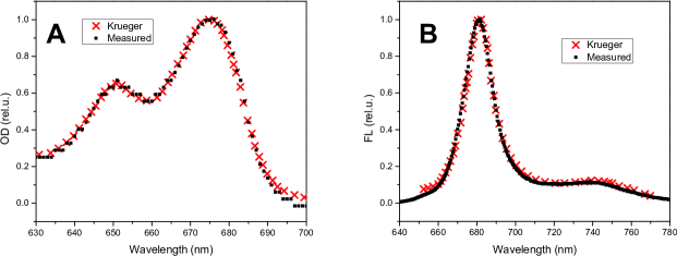
Figure S1: Bulk spectra measured and taken from Ref. Kruger2010

Random Walk Model

In the original description by Valkunas Valkunas2012 and, in more detail, in Chmeliov2013 , the protein diffusive motion was described as a continuous-time random walk (CTRW) on a two-dimensional potential energy surface. Here we somewhat simplify this description in the following way. The two generalized coordinates represent fast and slow degrees of freedom and thus, when following the slow dynamics, the fast fluctuations can be adiabatically eliminated. It can be shown that when we consider the potential dependence on the fast coordinate the same in both the on and off states for simplicity, i.e. setting $x_{0}=0,\>\nicefrac{{\lambda_{2}}}{{\lambda_{1}}}=1$ in Valkunas2012 , the fast coordinate can be completely removed. This leaves us with effectively one-dimensional problem.

After transforming into dimensionless coordinates $y\sqrt{\frac{\gamma_{1}}{k_{B}T}}\rightarrow y$, the parabolically approximated minima of the potential for the on (1) and off (2) state are

$$\frac{U_{1}}{k_{B}T} = \frac{1}{2}y^{2},$$

$$\frac{U_{2}}{k_{B}T} = \frac{1}{2}\frac{\gamma_{2}}{\gamma_{1}}\left(y-y_{0}\right)^{2}+\frac{U_{0}}{k_{B}T}.$$ (27)

Here $\gamma_{1,2}$ determine the steepness of the potential and the second minimum is shifted by $y_{0}$ along the slow coordinate and by $U_{0}$ along the potential energy.

The protein then performs random walk on the respective surface, with probabilities to tunnel to the other surface

$$\kappa_{1\rightarrow 2}(y) =k_{1} e^{-\alpha|U_{1}-U_{2}|/\hbar\omega_{0}}\mbox{min$\{1,e^{(U_{1}-U_{2})/k_{B}T}$}\},$$

$$\kappa_{2\rightarrow 1}(y) =k_{2} e^{-\alpha|U_{1}-U_{2}|/\hbar\omega_{0}}\mbox{min$\{1,e^{(U_{2}-U_{1})/k_{B}T}$}\}.$$ (28)

$k_{i}$ is a rate of falling from the $i-th$ potential, the first exponential term reflects the energy gap law and the min term ensures detailed balance condition. The coefficient $\alpha$ can be treated as a constant and $\omega_{0}$ is a characteristic frequency of the protein environment vibrations responsible for the tunneling.

The protein diffusion under this conditions can be described either by the CTRW or by a discrete random walk (RW). The former approach was employed by Valkunas et al.Valkunas2012 ; Chmeliov2013 . However, we believe that for our purpose it is better to solve this problem as a discrete RW for two reasons. First, the coupled Smoluchovski equations for the CTRW on the two potentials can be decoupled only for conditional probabilities, i.e. assuming that the system was in the opposite state in the previous interval, and, in the same time, employing the same, equilibrium initial condition for each dwell time. When continuously modelling the trajectory of a single protein, we do not have to include the resetting after switching and also the conditioning will be inherent, as the system is observed being in a particular state. And second, when we want to simulate the individual intensity time traces, it is more natural to really follow the trajectories of the individual proteins on their PES.

If we want to follow the time trace of every single molecule, we should follow its particular trajectory. The blinking statistics will then be recovered by averaging over a large number of molecules, exactly as in the experiment. To the purpose of following trajectories of individual proteins, we need to describe its discrete RW (DRW) in the potential. We will denote probability of going right (left) as $p$ ($q$). In the symmetrical RW we have $p=q=\frac{1}{2}$. If the protein is at a coordinate $y$, in the next step it will move with probability $p$ to $y+a$ and with probability $q$ to $y-a$, where $a$ is the length of the step. Inspired by classical approach by van Kampen vanKampen , we augment the position dependent probabilities in the presence of the potential $U(y)$ as

$$p(y) = \frac{1}{2}e^{-\frac{1}{k_{B}T}\left(U(y+a)-U(y)\right)},$$

$$q(y) = \frac{1}{2}e^{-\frac{1}{k_{B}T}\left(U(y-a)-U(y)\right)}.$$ (29)

We note that defined probabilities defined in Eq. (29) reflect the detailed balance condition $\frac{p(y)}{q(y)}=e^{-\frac{1}{k_{B}T}\left(U(y+a)-U(y-a)\right)}$. Considering a small step $a$, we can use Taylor expansion in $y$ $\left(e^{-\frac{1}{k_{B}T}U(y\pm a)}\approx e^{-\frac{1}{k_{B}T}U(y)}\left(1\mp\frac{1}{k_{B}T}\frac{dU}{dy}(y)a\right)\right)$, obtaining

$$p(y)-q(y)=-\frac{1}{k_{B}T}\frac{dU}{dy}(y)a.$$ (30)

Now, considering that $p(y)+q(y)=1$, we get

$$p(y)=\frac{1}{2}-\frac{1}{2k_{B}T}\frac{dU(y)}{dy}a.$$ (31)

Using the potential form (27), we get for the probabilities

$$p_{1}(y) = \frac{1}{2}-\frac{1}{2k_{B}T}ya_{1},$$

$$p_{2}(y) = \frac{1}{2}-\frac{1}{2k_{B}T}\frac{\gamma_{2}}{\gamma_{1}}(y-y_{0})a_{2}.$$ (32)

The length of the step $a$ on respective surface can be related to the transformed diffusion coefficient $D_{1,2}$:

$$a_{1,2}=\sqrt{\frac{D_{1,2}\gamma_{1}}{k_{B}T}\Delta t},$$ (33)

where $\Delta t$ is the time duration of the step. During $\Delta t$ the protein walks either to the left or right with the respective probability and with the probability $\kappa_{i\rightarrow j}(y)\Delta t$ switches to the other surface.

Similarly to Valkunas2012 the position near the potential intersection can be chosen as an initial condition. However, as we do not include resetting after switching in our approach, this determines only the starting point of each trajectory and is therefore not of significant importance. In Table 1 we present the parameters of our RW model compared to the ones used by Valkunas et al Valkunas2012 . Considering the differences - LHCII monomers vs trimers, discrete vs continuous RW, no resetting vs resetting - the agreement is satisfactory.

parameter	Valkunas (Valkunas2012, , pH 8)	This work
$\nicefrac{{\lambda_{2}}}{{\lambda_{1}}}$	0.2	1.0
$\nicefrac{{\gamma_{2}}}{{\gamma_{1}}}$	0.72	0.72
$x_{0}\sqrt{\nicefrac{{\lambda_{1}}}{{k_{B}T}}}$	1.0	0.0
$y_{0}\sqrt{\nicefrac{{\gamma_{1}}}{{k_{B}T}}}$	8.57	6.07
$\nicefrac{{U_{0}}}{{k_{B}T}}$	1.5	1.5
$k_{1}^{-1}$	430 ms	330 ms
$k_{2}^{-1}$	4.8 ms	50 ms
$\left(D_{1}\nicefrac{{\gamma_{1}}}{{k_{B}T}}\right)^{-1}$	3.8 s	66 s
$\left(D_{2}\nicefrac{{\gamma_{1}}}{{k_{B}T}}\right)^{-1}$	1.4 s	10 s
$\nicefrac{{\hbar\omega_{0}}}{{\alpha k_{B}T}}$	1.0	1.0

Table 1: RW model parameters

References

- (1) Blankenship, R. E. Molecular Mechanisms of Photosynthesis (Blackwell Science, 2002).
- (2) Wraight, C. A. & Clayton, R. K. The absolute quantum efficiency of bacteriochlorophyll photooxidation in reaction centres of Rhodopseudomonas spheroides. Biochim. Biophys. Acta - Bioenerg. 333, 246–260 (1974).
- (3) Blankenship, R. E. et al. Comparing photosynthetic and photovoltaic efficiencies and recognizing the potential for improvement. Science 332, 805–809 (2011).
- (4) van Amerongen, H., van Grondelle, R. & Valkunas, L. Photosynthetic Excitons (World Scientific, London, 2000).
- (5) Ruban, A. V., Johnson, M. P. & Duffy, C. D. P. The photoprotective molecular switch in the photosystem II antenna. Biochim. Biophys. Acta - Bioenerg. 1817, 167–181 (2012).
- (6) Holt, N. E. et al. Carotenoid cation formation and the regulation of photosynthetic light harvesting. Science 307, 433–436 (2005).
- (7) Ruban, A. V. et al. Identification of a mechanism of photoprotective energy dissipation in higher plants. Nature 450, 575–8 (2007).
- (8) Avenson, T. J. et al. Zeaxanthin radical cation formation in minor light-harvesting complexes of higher plant antenna. J. Biol. Chem. 283, 3550–3558 (2008).
- (9) Bode, S. et al. On the regulation of photosynthesis by excitonic interactions between carotenoids and chlorophylls. Proc. Natl. Acad. Sci. U. S. A. 106, 12311–12316 (2009).
- (10) Berera, R., Van Stokkum, I. H. M., Kennis, J. T. M., Grondelle, R. V. & Dekker, J. P. The light-harvesting function of carotenoids in the cyanobacterial stress-inducible IsiA complex. Chem. Phys. 373, 65–70 (2010).
- (11) Müller, M. G. et al. Singlet energy dissipation in the photosystem II light-harvesting complex does not involve energy transfer to carotenoids. Chemphyschem 11, 1289–96 (2010).
- (12) Fuciman, M. et al. The Role of Xanthophylls in Light-Harvesting in Green Plants: A Spectroscopic Investigation of Mutant LHCII and Lhcb Pigment-Proteins Complexes. J. Phys. Chem. B 116, 3834–49 (2012).
- (13) Staleva, H. et al. Mechanism of photoprotection in the cyanobacterial ancestor of plant antenna proteins. Nat. Chem. Biol. 11 (2015).
- (14) Haarer, D. & Silbey, R. Hole-Burning Spectroscopy of Glasses. Phys. Today 43, 58 (1990).
- (15) Johnson, S., Tang, D., Jankowiak, R., Hayes, J. M. & Small, G. J. Structure and marker mode of the primary electron donor state absorption of photosynthetic bacteria: hole-burned spectra. J. Phys. Chem. 93, 5953–5957 (1989).
- (16) Creemers, T. M. H., Caro, C. A. D., Visschers, R. W., Grondelle, R. V. & Vo, S. Spectral Hole Burning and Fluorescence Line Narrowing in Subunits of the Light-Harvesting Complex LH1 of Purple Bacteria. J. Phys. Chem. B 103, 9770–9776 (1999).
- (17) Jonas, D. M. Two-dimensional femtosecond spectroscopy. Annu. Rev. Phys. Chem. 54, 425–463 (2003).
- (18) Moerner, W. & Kador, L. Optical detection and spectroscopy of single molecules in a solid. Phys. Rev. Lett. 62, 2535–2538 (1989).
- (19) Schlau-Cohen, G. S. et al. Single-Molecule Identification of Quenched and Unquenched States of LHCII. J. Phys. Chem. Lett. 860–867 (2015).
- (20) Liu, Z. et al. Crystal structure of spinach major light-harvesting complex at 2 . 72 A resolution. Nature 428, 287–292 (2004).
- (21) Novoderezhkin, V. I., Palacios, M. A., van Amerongen, H. & van Grondelle, R. Energy-Transfer Dynamics in the LHCII Complex of Higher Plants: Modified Redfield Approach. J. Phys. Chem. B 108, 10363 (2004).
- (22) Novoderezhkin, V. I., Palacios, M. A., van Amerongen, H. & van Grondelle, R. Excitation dynamics in the LHCII complex of higher plants: modeling based on the 2.72 Angstrom crystal structure. J. Phys. Chem. B 109, 10493–504 (2005).
- (23) Novoderezhkin, V., Marin, A. & Grondelle, R. V. Supplementary Information Intra- and inter-monomeric transfers in the light harvesting LHCII complex : the Redfield-Förster picture (2011).
- (24) Krüger, T. P. J., Novoderezhkin, V. I., Ilioaia, C. & van Grondelle, R. Fluorescence spectral dynamics of single LHCII trimers. Biophys. J. 98, 3093–101 (2010).
- (25) Tietz, C. et al. Single molecule spectroscopy on the light-harvesting complex II of higher plants. Biophys. J. 81, 556–62 (2001).
- (26) Krüger, T. P. J., Ilioaia, C., Valkunas, L. & van Grondelle, R. Fluorescence intermittency from the main plant light-harvesting complex: sensitivity to the local environment. J. Phys. Chem. B 115, 5083–95 (2011).
- (27) Krüger, T. P. J. et al. Controlled disorder in plant light-harvesting complex II explains its photoprotective role. Biophys. J. 102, 2669–76 (2012).
- (28) Krüger, T. P. J., Ilioaia, C. & van Grondelle, R. Fluorescence intermittency from the main plant light-harvesting complex: resolving shifts between intensity levels. J. Phys. Chem. B 115, 5071–82 (2011).
- (29) Malý, P., Gruber, J. M., Cogdell, R. J., Mančal, T. & van Grondelle, R. Ultrafast Energy Relaxation in Single Light-Harvesting Complexes. arXiv:1511.04936[physics.bio-ph] (2015).
- (30) May, V. & Kühn, O. Charge and Energy Transfer Dynamics in Molecular Systems (Wiley-VCH, 2011).
- (31) Valkunas, L., Abramavicius, D. & Mančal, T. Molecular Excitation Dynamics and Relaxation (Wiley-VCH, 2013).
- (32) Ishizaki, A. & Fleming, G. R. Unified treatment of quantum coherent and incoherent hopping dynamics in electronic energy transfer: reduced hierarchy equation approach. J. Chem. Phys. 130, 234111 (2009).
- (33) Hein, B., Kreisbeck, C., Kramer, T. & Rodríguez, M. Modelling of oscillations in two-dimensional echo-spectra of the Fenna-Matthews-Olson complex. New J. Phys. 14, 023018 (2012).
- (34) Wilkins, D. M. & Dattani, N. S. Why quantum coherence is not important in the Fenna-Matthews-Olsen Complex. J. Chem. Theory Comput. 150304125043002 (2015).
- (35) Prior, J., Chin, A. W., Huelga, S. F. & Plenio, M. B. Efficient simulation of strong system-environment interactions. Phys. Rev. Lett. 105, 1–4 (2010).
- (36) Shi, Q. & Geva, E. A semiclassical generalized quantum master equation for an arbitrary system-bath coupling. J. Chem. Phys. 120, 12063 (2004).
- (37) Stockburger, J. T. & Grabert, H. Exact c-number representation of non-Markovian quantum dissipation. Phys. Rev. Lett. 88, 170407 (2002).
- (38) Xu, R. X., Cui, P., Li, X. Q., Mo, Y. & Yan, Y. Exact quantum master equation via the calculus on path integrals. J. Chem. Phys. 122, 041103 (2005).
- (39) Huo, P., Bonella, S., Chen, L. & Coker, D. F. Linearized approximations for condensed phase non-adiabatic dynamics: Multi-layered baths and Brownian dynamics implementation. Chem. Phys. 370, 87–97 (2010).
- (40) Schröter, M. et al. Exciton-vibrational coupling in the dynamics and spectroscopy of Frenkel excitons in molecular aggregates. Phys. Rep. 567, 1–78 (2014).
- (41) Fain, B. Irreversibilities in Quantum Mechanics (Kluer Acadenic Publishers, Dorderecht, 2000).
- (42) Jiang, X.-p. & Brumer, P. Creation and dynamics of molecular states prepared with coherent vs partially coherent pulsed light. J. Chem. Phys. 94, 5833–5843 (1991).
- (43) Mančal, T. & Valkunas, L. Exciton dynamics in photosynthetic complexes: Excitation by coherent and incoherent light. New J. Phys. 12, 1–12 (2010).
- (44) Brumer, P. & Shapiro, M. Molecular response in one-photon absorption via natural thermal light vs. pulsed laser excitation. Proc. Natl. Acad. Sci. U. S. A. 109, 19575–8 (2012).
- (45) Chenu, A., Malý, P. & Mančal, T. Dynamic coherence in excitonic molecular complexes under various excitation conditions. Chem. Phys. 439, 100–110 (2014).
- (46) Mančal, T. & Šanda, F. Quantum master equations for non-linear optical response of molecular systems. Chem. Phys. Lett. 530, 140–144 (2012).
- (47) Olšina, J. & Mančal, T. Parametric projection operator technique for second order non-linear response. Chem. Phys. 404, 103–115 (2012).
- (48) Mukamel, S. Principles of nonlinear spectroscopy (Oxford University Press, Oxford, 1995).
- (49) Page, C. H. Instantaneous Power Spectra. J. Appl. Phys. 23, 103 (1952).
- (50) Peterman, E. J. G., Pullerits, T., Van Grondelle, R. & Van Amerongen, H. Electron-phonon coupling and vibronic fine structure of light-harvesting complex II of green plants: Temperature dependent absorption and high-resolution fluorescence spectroscopy. J. Phys. Chem. B 101, 4448–4457 (1997).
- (51) Nordlund, T. M. & Knox, W. H. Lifetime of Fluorescence from Light-Harvesting Chlorophyll a/b proteins. Biophys. J. 36, 193–201 (1981).
- (52) Schodel, R., Irrgang, K. D., Voigt, J. & Renger, G. Rate of carotenoid triplet formation in solubilized light-harvesting complex II (LHCII) from spinach. Biophys. J. 75, 3143–53 (1998).
- (53) Duffy, C. D. P. et al. Modeling of fluorescence quenching by lutein in the plant light-harvesting complex LHCII. J. Phys. Chem. B 117, 10974–86 (2013).
- (54) Polívka, T., Zigmantas, D. & Sundström, V. Carotenoid S1 State in a Recombinant Light-Harvesting Complex of Photosystem II. Biochemistry 41, 439 (2002).
- (55) Valkunas, L., Chmeliov, J., Krüger, T. P. J., Ilioaia, C. & van Grondelle, R. How Photosynthetic Proteins Switch. J. Phys. Chem. Lett. 3, 2779–2784 (2012).
- (56) Chmeliov, J., Valkunas, L., Krüger, T. P. J., Ilioaia, C. & van Grondelle, R. Fluorescence blinking of single major light-harvesting complexes. New J. Phys. 15, 85007 (2013).
- (57) Chmeliov, J. et al. An ’all pigment’ model of excitation quenching in LHCII. Phys. Chem. Chem. Phys. 17, 15857–15867 (2015).
- (58) Barkai, E., Brown, F. L. H., Orrit, M. & Yang, H. (eds.) Theory and Evaluation of Single-Molecule Signals (World Scientific, 2008).
- (59) Van Roon, H., Van Breemen, J. F. L., De Weerd, F. L., Dekker, J. P. & Boekema, E. J. Solubilization of green plant thylakoid membranes with n-dodecyl-a,D-maltoside. Implications for the structural organization of the Photosystem II, Photosystem I, ATP synthase and cytochrome b6f complexes. Photosynth. Res. 64, 155–166 (2000).
- (60) Nussberger, S. et al. Spectroscopic characterization of three different monomeric forms of the main chlorophyll a/b binding protein from chloroplast membranes. Biochemistry 33, 14775–14783 (1994).
- (61) van Kampen, N. G. Stochastic processes in physics and chemistry (North Holland, 1992).
Acknowledgments
P.M., J.M.G. and R.v.G. were supported by the VU University and by an Advanced Investigator grant from the European Research Council (no. 267333, PHOTPROT) to R.v.G.; R.v.G. was also supported by the Nederlandse Organisatie voor Wetenschappelijk Onderzoek, Council of Chemical Sciences (NWO-CW) via a TOP-grant (700.58.305), and by the EU FP7 project PAPETS (GA 323901). R.v.G. gratefully acknowledges his Academy Professor grant from the Netherlands Royal Academy of Sciences (KNAW). P.M. and T.M. received financial support from the Czech Science Foundation (GACR), grant no. 14-25752S. T. M. acknowledges the kind support of the Nederlandse Organisatie voor Wetenschappelijk Onderzoek (NWO) visitor grant nr. 040.11.423 during his stay at the VU Amsterdam.