Improved fractal Weyl bounds
for hyperbolic manifolds

Abstract.

We give a new fractal Weyl upper bound for resonances of convex co-compact hyperbolic manifolds in terms of the dimension $n$ of the manifold and the dimension $\delta$ of its limit set. More precisely, we show that as $R\to\infty$, the number of resonances in the box $[R,R+1]+i[-\beta,0]$ is $\mathcal{O}(R^{m(\beta,\delta)+})$, where the exponent $m(\beta,\delta)=\min(2\delta+2\beta+1-n,\delta)$ changes its behavior at $\beta={n-1\over 2}-{\delta\over 2}$. In the case $\delta<{n-1\over 2}$, we also give an improved resolvent upper bound in the standard resonance free strip $\{\operatorname{Im}\lambda>\delta-{n-1\over 2}\}$. Both results use the fractal uncertainty principle point of view recently introduced in [DyZa]. The appendix presents numerical evidence for the Weyl upper bound.

In this paper we study asymptotics of scattering resonances of convex co-compact hyperbolic quotients $(M,g)=\Gamma\backslash\mathbb{H}^{n}$. Resonances are complex numbers which replace eigenvalues as discrete spectral data of the Laplacian for non-compact manifolds – see for instance [Bo16, DyZw]. They are defined as poles of the scattering resolvent

$$\mathcal{R}(\lambda)=\Big{(}-\Delta_{g}-{(n-1)^{2}\over 4}-\lambda^{2}\Big{)}^{-1}:L^{2}_{\operatorname{comp}}(M)\to H^{2}_{\operatorname{loc}}(M),\quad\lambda\in\mathbb{C},$$ (1.1)

which is the meromorphic continuation of the $L^{2}$ resolvent from the upper half-plane – see §2.2. Resonances correspond to zeroes of the Selberg zeta function [GLZ, (3.1)]

$$Z_{\Gamma}(s)=\prod_{\gamma}\prod_{\alpha\in\mathbb{N}_{0}^{n-1}}\Big{(}1-e^{-i\langle\theta(\gamma),\alpha\rangle}e^{-(s+|\alpha|)\ell(\gamma)}\Big{)},\quad s={n-1\over 2}-i\lambda,$$ (1.2)

where $\gamma$ varies in the set of primitive closed geodesics on $M$, $\ell(\gamma)$ is its period, and $\theta(\gamma)$ its holonomy spectrum – see [GLZ] for details.

Our main result is a bound on the number of resonances in strips, using the quantity

$$\mathcal{N}(R,\beta)=\#\{\lambda\text{ resonance},\ \operatorname{Re}\lambda\in[R,R+1],\ \operatorname{Im}\lambda\geq-\beta\},\quad R,\beta>0.$$

Theorem 1.

Let $\delta\in[0,n-1]$ be the dimension of the limit set of $\Gamma$, see e.g. [DyZa, (5.2)]. Then for each $\beta\geq 0,\varepsilon>0$, there exists a constant $C$ such that

$$\mathcal{N}(R,\beta) \leq CR^{m(\beta,\delta)+\varepsilon},\quad R\to\infty;$$ (1.3)

$$m(\beta,\delta) :=\min(2\delta+2\beta+1-n,\delta).$$ (1.4)

Here resonances are counted with multiplicities, see (4.2).

See Figure 1(a),(b). In the Appendix, we compare this upper bound with numerically computed resonance data for several examples of hyperbolic surfaces.

The bound (1.3) is related to several previous results on distribution of resonances (see [Non] for a more broad overview of results in open quantum chaos):

  (a) (b) (c)

Figure 1. (a),(b) Plots of the exponent $m(\beta,\delta)$ in the Weyl bound (1.3), for $n=2$ and (a) $\delta=0.6$ (b) $\delta=0.4$. (c) Plot of the exponent $c(\beta,\delta)$ in the resolvent bound (1.10), for $n=2$ and $\delta=0.15$. The straight lines are the previous resolvent bound $c=2\beta$ of [DyZa] and the lower bound $c=\beta$ of [DyWa].

1. The bound

$$\mathcal{N}(R,\beta)\leq CR^{\delta},\quad R\to\infty$$ (1.5)

was proved by Guillopé–Lin–Zworski [GLZ] for convex co-compact Schottky quotients, including all convex co-compact hyperbolic surfaces. (See also the earlier work of Zworski [Zw99] in the case of surfaces.) Datchev–Dyatlov [DaDy] proved (1.5) for all convex co-compact hyperbolic quotients and a wider class of asymptotically hyperbolic manifolds with hyperbolic trapped sets, using the methods developed by Sjöstrand [Sj] and Sjöstrand–Zworski [SjZw] in the case of Euclidean infinite ends. Note that in contrast with (1.3), the bound (1.5) does not lose an $\varepsilon$ in the exponent.

2. The standard Patterson–Sullivan spectral gap [Pa, Su] states that for $\delta<{n-1\over 2}$, there are no resonances in $\{\operatorname{Im}\lambda>\delta-{n-1\over 2}\}$, that is

$$\mathcal{N}(R,\beta)=0,\quad\beta<{n-1\over 2}-\delta.$$

This is in agreement with the fact that $m(\beta,\delta)<0$ when $\beta<{n-1\over 2}-\delta$. Essential gaps of larger size (depending in a complicated way on the quotient) have been obtained by Naud [Na05], Stoyanov [St], and Dyatlov–Zahl [DyZa].

3. In [JaNa12], Jakobson and Naud have conjectured an essential gap of size ${n-1-\delta\over 2}$:

$$\mathcal{N}(R,\beta)=0,\quad\beta<{n-1-\delta\over 2},\quad R\gg 1.$$

While numerical evidence does not seem to confirm this conjecture, it does show that the set of resonances becomes more dense near the line $\operatorname{Im}\lambda=-{n-1-\delta\over 2}$ – see the works of Borthwick [Bo14, §§7,8], Borthwick–Weich [BoWe, §5.3], and the Appendix. This is a special case of concentration of imaginary parts of resonances near the pressure ${1\over 2}P(1)$ for open chaotic systems, first discovered numerically by Lu–Sridhar–Zworski [LSZ, Figure 2] for semiclassical zeta functions on multi-disk scatterers and later observed in microwave experiments by Barkhofen et al. [BWPSKZ, Figure 4]. In the setting of open quantum maps, such concentration was observed numerically by Shepelyanski [Sh, Figures 4 and 5] and Novaes [Nov]; the recent work of Dyatlov–Jin [DyJi16] proves an analog of Theorem 1 for quantum open baker’s maps. Our exponent (1.4) is in agreement with these observations, since it changes behavior at $\beta={n-1-\delta\over 2}$.

4. In [Na14], Naud obtained an improved Weyl upper bound in dimension $n=2$,

$$\mathcal{N}(R,\beta)\leq CR^{m^{\prime}(\beta,\delta)},\quad R\to\infty,$$

where $m^{\prime}(\beta,\delta)$ is some function satisfying

$$m^{\prime}(\beta,\delta)<\delta\quad\text{for }\beta<{1-\delta\over 2}.$$

This result was extended to uniform bounds for congruence subgroups of arithmetic groups by Jakobson–Naud [JaNa16]. These bounds make essential use of total discontinuity of the limit set, apply to surfaces only, and depend on the choice of a particular Schottky representation of $\Gamma$; we also note that unlike (1.4), $m^{\prime}(\beta,\delta)$ is positive at the Patterson–Sullivan gap $\beta={1\over 2}-\delta$. The exponent in Theorem 1 is always smaller than the ones obtained in [Na14, JaNa16] – see (A.6) and (A.7).

5. We finally discuss known lower bounds on the number of resonances in strips. Guillope–Zworski [GuZw99] showed that for $n=2$, the number of resonances in $[0,R]+i[-\beta,0]$ cannot be $\mathcal{O}(R^{1-1/\beta})$, for $\beta>2$. A similar result for higher dimensional manifolds was proved by Perry [Pe03]. Jakobson–Naud [JaNa12] proved that there are infinitely many resonances in $\{\operatorname{Im}\lambda>-\beta\}$, for $\beta=(2\delta^{2}-\delta+1)/2$ for surfaces and $\beta={3\over 4}-{\delta\over 2}$ for the special class of arithmetic surfaces with $\delta>{1\over 2}$. Neither of these bounds matches (1.3), since they give no information for $\beta<{1-\delta\over 2}$ and the exponents of $R$ in the lower bounds are much smaller than $\delta$. However, numerical computations indicate that the bound (1.3) is saturated at least when $\beta>{n-1-\delta\over 2}$ – see the Appendix. See also [PWBKSZ] for experimental data in the related case of many-disk scattering.

Outline of the proof of Theorem 1. Theorem 1 is proved in §4; we give an informal outline of the proof here. We use the semiclassically rescaled spectral parameter $\omega=h\lambda$, putting $h:=R^{-1}\ll 1$.

Assume first that $\lambda=\omega/h$ is a resonance, then there exists a resonant state

$$u\in C^{\infty}(M),\quad\Big{(}-h^{2}\Delta_{g}-{h^{2}(n-1)^{2}\over 4}-\omega^{2}\Big{)}u=0,\quad u\text{ outgoing}.$$

The outgoing condition can be formulated in terms of asymptotics of $u$ at the infinite ends of $M$. We use the recent approach due to Vasy [Va1, Va2] (as reviewed in §2.2; see [DyZw, Chapter 5] and [Zw16] for expository treatments) which multiplies $u$ by a power of the boundary defining function at conformal infinity and extends it past the boundary of the even compactification of $M$, to obtain a smooth function on a compact manifold without boundary $M_{\mathrm{ext}}\supset M$. The semiclassical scattering resolvent $R_{h}(\omega)=h^{-2}R(\omega/h)$ is expressed via the inverse of a family of Fredholm operators (denoted $\mathcal{P}_{h}(\omega)$ in this paper) on a Sobolev space on $M_{\mathrm{ext}}$. We denote by $\|u\|$ the norm of its extension to $M_{\mathrm{ext}}$ in this Sobolev space. We reduce the analysis to a compact region inside the original manifold $M$, essentially treating the construction of [Va1, Va2] as a black box.

Let $\Gamma_{\pm}\subset T^{*}M$ be the incoming/outgoing tails and $K=\Gamma_{+}\cap\Gamma_{-}$ the trapped set, see §2.1. It follows immediately from [Va1, Va2] that $u$ is microlocally concentrated on $\Gamma_{+}\cap\{|\xi|_{g}=1\}$; in particular, for each $h$-independent symbol $a(x,\xi)\in C_{0}^{\infty}(T^{*}M)$ and $\operatorname{Op}_{h}(a)$ the corresponding semiclassical pseudodifferential operator (see [Zw12]), we have

$$\operatorname{supp}a\cap\Gamma_{+}\cap\{|\xi|_{g}=1\}=\emptyset\ \Longrightarrow\ \|\operatorname{Op}_{h}(a)u\|=\mathcal{O}(h^{\infty})\|u\|.$$

It was shown in [DyZa, §4.3] (modulo localization to the cosphere bundle $\{|\xi|_{g}=1\}$, which is proved in Lemma 2.8) that $u$ is in fact microlocalized $h^{\rho}$ close to $\Gamma_{+}\cap\{|\xi|_{g}=1\}$, for any $\rho<1$: namely there exists

$$\chi_{+}(x,\xi;h)\in C_{0}^{\infty}(T^{*}M),\quad\operatorname{supp}\chi_{+}\subset Ch^{\rho}\text{-neighborhood of }\Gamma_{+}\cap\{|\xi|_{g}=1\},$$

such that (assuming for simplicity that $\operatorname{Op}_{h}^{L_{u}}(1)$ is the identity operator; see the next paragraph for the notation $\operatorname{Op}_{h}^{L_{u}}$)

$$u=\operatorname{Op}_{h}^{L_{u}}(\chi_{+})u+\mathcal{O}(h^{\infty})\|u\|\quad\text{microlocally near }K.$$ (1.6)

In practice, we will take $\rho$ very close to 1. The derivatives of the symbol $\chi_{+}$ grow like $h^{-\rho}$, therefore it cannot be quantized using standard pseudodifferential calculus. However, $\Gamma_{+}\cap\{|\xi|_{g}=1\}$ is foliated by the leaves of the weak unstable foliation $L_{u}$ (see (2.1)), and $\chi_{+}$ does not grow when differentiated along $L_{u}$. This makes it possible to quantize $\chi_{+}$ using the quantization procedure $\operatorname{Op}_{h}^{L_{u}}$ developed in [DyZa], see §2.3.

Furthermore, [DyZa, §4.3] shows that $u$ cannot be too small on $\Gamma_{-}$: there exists

$$\chi_{-}(x,\xi;h)\in C_{0}^{\infty}(T^{*}M),\quad\operatorname{supp}\chi_{-}\subset Ch^{\rho}\text{-neighborhood of }\Gamma_{-},$$

such that (modulo an arbitrarily small loss in the power of $h$)

$$\|u\|\leq Ch^{\rho\operatorname{Im}\omega/h}\|\operatorname{Op}_{h}^{L_{s}}(\chi_{-})u\|.$$ (1.7)

Here we again use the calculus of [DyZa, §3], this time associated to the weak stable foliation $L_{s}$. Together, (1.6) and (1.7) give

$$\|u\|\leq Ch^{\rho\operatorname{Im}\omega/h}\|\operatorname{Op}_{h}^{L_{s}}(\chi_{-})\operatorname{Op}_{h}^{L_{u}}(\chi_{+})u\|.$$ (1.8)

In [DyZa], an operator norm bound on the product $\operatorname{Op}_{h}^{L_{s}}(\chi_{-})\operatorname{Op}_{h}^{L_{u}}(\chi_{+})$ (called the fractal uncertainty principle) was used to show an essential spectral gap. In the present paper, we give a stronger version of (1.8), Proposition 2.1, which constructs a smoothing operator

$$\mathcal{A}(\omega)=\mathcal{J}(\omega)\operatorname{Op}_{h}^{L_{s}}(\chi_{-})\operatorname{Op}_{h}^{L_{u}}(\chi_{+})+\mathcal{O}(h^{\infty}),\quad\|\mathcal{J}(\omega)\|\leq Ch^{\rho\operatorname{Im}\omega/h},$$

such that if $\lambda=\omega/h$ is a resonance, then $1-\mathcal{A}(\omega)$ is not invertible. Then each resonance produces a zero of the Fredholm determinant

$$F(\omega)=\det(1-\mathcal{A}(\omega)^{2}).$$

By Jensen’s inequality, to show (1.3) with $m=2\delta+2\beta+1-n$ it remains to prove the Hilbert–Schmidt bound (see Proposition 3.1)

$$\|\mathcal{A}(\omega)\|_{\operatorname{HS}}^{2}\leq Ch^{2\operatorname{Im}\omega/h+n-1-2\delta-\varepsilon}.$$

The term $h^{2\operatorname{Im}\omega/h}$ comes from the operator norm of $\mathcal{J}(\omega)$, thus it remains to show

$$\|\operatorname{Op}_{h}^{L_{s}}(\chi_{-})\operatorname{Op}_{h}^{L_{u}}(\chi_{+})\|_{\operatorname{HS}}^{2}\leq Ch^{n-1-2\delta-\varepsilon}.$$ (1.9)

The latter estimate can be heuristically explained as follows: since both $\chi_{\pm}$ are bounded, the left-hand side of (1.9) should behave like $h^{-n}$ times the volume in $T^{*}M$ of the set $\operatorname{supp}\chi_{-}\cap\operatorname{supp}\chi_{+}$. Locally near any point in $K\cap\{|\xi|_{g}=1\}$, we may view this set as the product of (here $\Lambda_{\Gamma}\subset\mathbb{S}^{n-1}$ denotes the limit set of the group):

1. an $h^{\rho}$ sized interval in the direction transversal to the energy surface;

2. a fixed size interval in the direction of the geodesic flow;

3. an $h^{\rho}$ neighborhood of $\Lambda_{\Gamma}$ in the stable direction, with volume $\mathcal{O}(h^{\rho(n-1-\delta)})$;

4. an $h^{\rho}$ neighborhood of $\Lambda_{\Gamma}$ in the unstable direction, with volume $\mathcal{O}(h^{\rho(n-1-\delta)})$.

Thus for $\rho=1$, the volume of $\operatorname{supp}\chi_{-}\cap\operatorname{supp}\chi_{+}$ is $\mathcal{O}(h^{2n-1-2\delta})$, finishing the proof.

To obtain (1.3) with $m=\delta$, we argue in the same way, but putting $\mathcal{A}(\omega)=\operatorname{Op}_{h}^{L_{u}}(\chi_{+})$ and using (1.6) only. The support of $\chi_{+}$ can be viewed as a product of the four sets above, with the set (4) replaced by a fixed size interval, thus for $\rho=1$ it has volume $\mathcal{O}(h^{n-\delta})$, leading to the Hilbert–Schmidt bound $\|\mathcal{A}(\omega)\|_{\operatorname{HS}}^{2}\leq Ch^{-\delta}$ and to (1.3).

The above proof shows why the exponent $m(\beta,\delta)$ changes behavior at $\beta={n-1-\delta\over 2}$: past this point, the growth as $h\to 0$ of $\|\mathcal{J}(\omega)\|^{2}$ is faster than the decay of the volume of the $h$-neighborhood of $\Gamma_{-}$, thus it is no longer benefical to use (1.7). Therefore, for $\beta<{n-1-\delta\over 2}$ we use localization on both $\Gamma_{+}$ and $\Gamma_{-}$ and for $\beta>{n-1-\delta\over 2}$, we only use localization on $\Gamma_{+}$.

Upper bounds on the resolvent. Using the strategy of the proof of Theorem 1 explained above, we also obtain the following resolvent bound inside the Patterson–Sullivan gap (see §4 for the proof):

Theorem 2.

Assume that $\delta<{n-1\over 2}$. Then for each $\beta\in(0,{n-1\over 2}-\delta)$, $\psi\in C_{0}^{\infty}(M)$, there exists $C_{0}$ such that for all $\varepsilon>0$,

$$\|\psi\mathcal{R}(\lambda)\psi\|_{L^{2}\to L^{2}}\leq C_{\varepsilon}|\lambda|^{-1+c(\beta,\delta)+\varepsilon},\quad\operatorname{Re}\lambda\geq C_{0},\quad\operatorname{Im}\lambda\in[-\beta,1],$$ (1.10)

where (see Figure 1(c))

$$c(\beta,\delta)={\beta(n-1-2\beta)\over n-1-\delta-2\beta}.$$ (1.11)

The estimate (1.10) with the power $c=2\beta$ was proved in [DyZa, Theorem 3 and (5.4)]. On the other hand, using the recent result of Dyatlov–Waters [DyWa, Theorem 1] (which applies to hyperbolic ends as explained in [DyWa, §1.2]; the Lyapunov exponent $\lambda_{\max}$ of the Hamiltonian flow $H_{|\xi|_{g}^{2}}$ on the sphere bundle is equal to 2), we see that (1.10) cannot hold with $c<\beta$. The value $c(\beta,\delta)$ given in (1.11) lies between these lower and upper bounds:

$$\beta\leq c(\beta,\delta)<2\beta\quad\text{for }\beta\in\Big{(}0,{n-1\over 2}-\delta\Big{)}.$$

Note that in the degenerate case $\delta=0$, we have $c(\beta,\delta)=\beta$, that is our upper bound matches the lower bound of [DyWa].

2. Approximate inverses

In this section, we review the framework for resonances on hyperbolic manifolds used in [DyZa]. We next construct an approximate inverse to the modified spectral family of the Laplacian, which is one of the key components of the proof – see Proposition 2.1.

2.1. Geometry and dynamics

Let $(M,g)$ be an $n$-dimensional convex co-compact hyperbolic manifold; see [Bo16] for the formal definition in dimension 2 and [Pe87] for general dimensions. Consider the function

$$p\in C^{\infty}(T^{*}M\setminus 0;\mathbb{R}),\quad p(x,\xi)=|\xi|_{g}.$$

The Hamiltonian flow

$$e^{tH_{p}}:T^{*}M\setminus 0\to T^{*}M\setminus 0$$

is the homogeneous version of the geodesic flow. This flow is hyperbolic in the sense that the tangent space $T(T^{*}M\setminus 0)$ decomposes into the stable, unstable, flow, and dilation directions, see [DyZa, (4.3)]. We will use the weak stable/unstable subbundles of $T(T^{*}M\setminus 0)$

$$L_{s}=\mathbb{R}H_{p}\oplus E_{s},\quad L_{u}=\mathbb{R}H_{p}\oplus E_{u},$$ (2.1)

see [DyZa, (4.6)]. By [DyZa, Lemma 4.1], $L_{s}$ and $L_{u}$ are Lagrangian foliations in the sense of [DyZa, Definition 3.1].

As in [DyZa, §4.1.2], consider a function

$$r:M\to\mathbb{R};\quad\ddot{r}>0\quad\text{on }\{r\geq 0\}\cap\{\dot{r}=0\}$$

where dots denote derivatives with respect to the flow $H_{p}$ of the lift of $r$ to $T^{*}M\setminus 0$. We moreover choose $r$ so that the sublevel sets $\{r\leq R\}$ are compact for all $R$. In fact, one may take $r:=\tilde{x}^{-1}-r_{1}$ where $\tilde{x}$ is the boundary defining function of a conformal compactification of $M$ and $r_{1}>0$ is a large constant. Then in the infinite ends of $M$, the function $r$ roughly behaves like the exponential of distance to the compact core.

Define the incoming/outgoing tails

$$\Gamma_{\pm}=\{(x,\xi)\in T^{*}M\setminus 0\mid r(e^{tH_{p}}(x,\xi))\text{ is bounded as }t\to\mp\infty\}$$

and the trapped set (which we assume to be nonempty)

$$K=\Gamma_{+}\cap\Gamma_{-}\ \subset\ \{r<0\}.$$

Then $\Gamma_{+}$ is foliated by the leaves of $L_{u}$ and $\Gamma_{-}$ is foliated by the leaves of $L_{s}$, as follows from [DyZa, (4.8) and (4.12)]. The intersection $K\cap\{|\xi|_{g}=c\}$ is compact for any constant $c$.

2.2. Scattering resolvent

The existence of the meromorphic continuation of the resolvent $\mathcal{R}(\lambda)$ defined in (1.1) was originally proved by Mazzeo–Melrose [MaMe], Guillarmou [Gu], and Guillopé–Zworski [GuZw95]; see [DyZa, §4.2] for more references. We use the recent approach of Vasy [Va1, Va2], refering to [DyZa, §4.2] for details and to [DyZw, Chapter 5], [Zw16] for expository treatments. This approach relies on semiclassical analysis; we refer the reader to [Zw12] and [DyZw, Appendix E] for an introduction to this subject and to [DyZa, §2] for the notation used here.

Consider the semiclassically rescaled resolvent

$$\mathcal{R}_{h}(\omega):=h^{-2}\mathcal{R}(\lambda),\quad\omega:=h\lambda\in\Omega,$$

where we fix $\beta_{0}>0$ and put

$$\Omega:=[1-2h,1+2h]+ih[-\beta_{0},1].$$ (2.2)

As in [Va1, Va2] and [DyZa, §4.2], we use the semiclassical differential operator

$$\mathcal{P}_{h}(\omega)\in\Psi^{2}_{h}(M_{\mathrm{ext}});\quad\mathcal{P}_{h}(\omega)=\psi_{2}\Big{(}-h^{2}\Delta_{g}-{h^{2}(n-1)^{2}\over 4}-\omega^{2}\Big{)}\psi_{1}\text{ on }M,$$ (2.3)

where $M_{\mathrm{ext}}$ is a compact $n$-dimensional manifold without boundary containing $M$ as an open subset and $\psi_{1},\psi_{2}\in C^{\infty}(M)$ are certain nonvanishing functions depending on $h,\omega$ and satisfying

$$\psi_{1}=\psi_{2}=1\quad\text{near }\{r\leq r_{0}\},$$ (2.4)

where $r_{0}>0$ can be fixed arbitrarily large; note that this implies

$$\sigma_{h}(\mathcal{P}_{h}(\omega))=p^{2}-\omega^{2}\quad\text{near }\{r\leq r_{0}\}.$$ (2.5)

Then (see for instance [Va2, Theorem 4.3]) $\mathcal{P}_{h}(\omega)$ is a family of Fredholm operators $\mathcal{X}\to\mathcal{Y}$ depending holomorphically on $\omega\in\Omega$, where

$$\mathcal{X}=\{u\in H^{s}_{h}(M_{\mathrm{ext}})\mid\mathcal{P}_{h}(1)u\in H^{s-1}_{h}(M_{\mathrm{ext}})\},\quad\mathcal{Y}:=H^{s-1}_{h}(M_{\mathrm{ext}}),$$

$s>{1\over 2}+\beta_{0}$ is fixed, and the $h$-dependent norm on $\mathcal{X}$ is defined as follows:

$$\|u\|_{\mathcal{X}}^{2}=\|u\|^{2}_{H^{s}_{h}(M_{\mathrm{ext}})}+\|\mathcal{P}_{h}(1)u\|^{2}_{H^{s-1}_{h}(M_{\mathrm{ext}})}.$$

By construction of the operator $\mathcal{P}_{h}(\omega)$, we have $\partial_{\omega}\mathcal{P}_{h}(\omega)\in\Psi^{1}_{h}(M_{\mathrm{ext}})$, implying that $\mathcal{P}_{h}(\omega)-\mathcal{P}_{h}(1)\in h\Psi^{1}_{h}(M_{\mathrm{ext}})$ for $\omega\in\Omega$. Therefore $\mathcal{P}_{h}(\omega)$ is bounded $\mathcal{X}\to\mathcal{Y}$ uniformly in $h$. Moreover, for each $u\in\mathcal{X}$, we have

$$\|u\|_{\mathcal{X}}\ \leq\ C\|u\|_{H^{s}_{h}(M_{\mathrm{ext}})}+C\|\mathcal{P}_{h}(\omega)u\|_{\mathcal{Y}}\ \leq\ C\|u\|_{H^{s+1}_{h}(M_{\mathrm{ext}})}.$$ (2.6)

The inverse $\mathcal{P}_{h}(\omega)^{-1}:\mathcal{Y}\to\mathcal{X}$ is meromorphic in $\omega\in\Omega$ (see for instance [Va2, Theorem 4.7]) and the rescaled scattering resolvent $\mathcal{R}_{h}(\omega)$ can be expressed via this inverse (see for instance [Va2, (5.2)]). Therefore, Theorem 1 follows from an upper bound on the number of poles of $\mathcal{P}_{h}(\omega)^{-1}$.

2.3. Approximate inverse statement

Our proofs rely on semiclassical analysis; we refer the reader to [Zw12] for a comprehensive introduction and to [DyZa, §2] for the notation used here. In particular we use

• the classical symbol classes $S^{k}(T^{*}M)$, $S^{k}_{h}(T^{*}M)$ and the corresponding class of pseudodifferential operators $\Psi^{k}_{h}(M)$;

• the principal symbol map $\sigma_{h}:\Psi^{k}_{h}(M)\to S^{k}(T^{*}M)$;

• the wavefront set $\operatorname{WF}_{h}(A)\subset\overline{T}^{*}M$ and the elliptic set $\operatorname{ell}_{h}(A)\subset\overline{T}^{*}M$ of $A\in\Psi^{k}_{h}(M)$ where $\overline{T}^{*}M$ is the fiber-radially compactified cotangent bundle;

• the class $\Psi^{\operatorname{comp}}_{h}(M)\subset\bigcap_{k}\Psi^{k}_{h}(M)$ of compactly supported and compactly microlocalized pseudodifferential operators.

We will moreover use the semiclassical calculus associated to a Lagrangian foliation developed in [DyZa, §3]. This calculus makes it possible to quantize $h$-dependent symbols $a\in C_{0}^{\infty}(U)$ which satisfy [DyZa, Definition 3.2]

$$\sup_{x,\xi}|Y_{1}\dots Y_{m}Z_{1}\dots Z_{k}a(x,\xi;h)|\leq Ch^{-\rho k},$$ (2.7)

for each vector fields $Y_{1},\dots,Y_{m},Z_{1},\dots,Z_{k}$ on $U$ such that $Y_{1},\dots,Y_{m}\in C^{\infty}(U;L)$. Here $\rho\in[0,1)$, $U\subset T^{*}M$ is an open subset, and $L$ is a Lagrangian foliation on $U$.

The class of symbols satisfying (2.7) is denoted by $S^{\operatorname{comp}}_{L,\rho}(U)$, and the resulting quantization procedure, by [DyZa, (3.11)]

$$a\in S^{\operatorname{comp}}_{L,\rho}(U)\ \mapsto\ \operatorname{Op}_{h}^{L}(a):\mathcal{D}^{\prime}(M)\to C_{0}^{\infty}(M).$$

We denote the corresponding class of operators by $\Psi^{\operatorname{comp}}_{h,L,\rho}(U)$. By [DyZa, Lemma 3.12], each $A\in\Psi^{\operatorname{comp}}_{h,L,\rho}(U)$ is pseudolocal and compactly microlocalized; that is, the wavefront set $\operatorname{WF}^{\prime}_{h}(A)$ is a compact subset of the diagonal of $T^{*}M$. Therefore, $A$ is bounded uniformly in $h$ as an operator $H^{-N}_{h}(M_{\mathrm{ext}})\to H^{N}_{h}(M_{\mathrm{ext}})$ for all $N$.

For symbols $a\in C_{0}^{\infty}(U)$ which belong to the class $S^{0}_{h}(T^{*}M)$ (in particular, all derivatives of $a$ are bounded uniformly in $h$), $\operatorname{Op}_{h}^{L}$ gives a quantization procedure for the class $\Psi^{\operatorname{comp}}_{h}(M)$ of standard compactly microlocalized semiclassical pseudodifferential operators.

Figure 2. The supports of the functions $\chi_{\pm}$, with thick lines depicting trajectories of the flow $e^{tH_{p}}$. The function $\chi_{+}$ additionally localizes to an $h^{\rho}$ neighborhood of the energy surface $\{|\xi|_{g}=1\}$.

We now introduce several cutoffs. Fix $h$-independent functions

$$\chi\in C_{0}^{\infty}(T^{*}M\setminus 0;[0,1]), \quad\chi=1\quad\text{near }K\cap\{|\xi|_{g}=1\};$$ (2.8)

$$\widetilde{\chi}\in C_{0}^{\infty}(\mathbb{R};[0,1]), \quad\widetilde{\chi}=1\quad\text{near }[-1,1].$$ (2.9)

Fix $\rho,\rho^{\prime}\in[0,1)$ and define $h$-dependent symbols $\chi_{\pm}\in C_{0}^{\infty}(T^{*}M\setminus 0;[0,1])$ by

$$\chi_{+} =\chi(\chi\circ e^{-\rho\log(1/h)H_{p}})\widetilde{\chi}\Big{(}{p-1\over h^{\rho}}\Big{)},$$ (2.10)

$$\chi_{-} =\chi(\chi\circ e^{\rho^{\prime}\log(1/h)H_{p}}).$$

In practice, we will take $\rho$ very close to $1$ depending on the value of $\varepsilon$ given in Theorem 1. We will take $\rho^{\prime}$ close to 1 to obtain the improved exponent $m(\beta)=2\delta+2\beta+1-n$ and close to $0$ to recover the standard exponent $m(\beta)=\delta$.

Near $K$, $\chi_{+}$ is a cutoff to an $h^{\rho}$ neighborhood of $\Gamma_{+}\cap\{|\xi|_{g}=1\}$ and $\chi_{-}$ is a cutoff to an $h^{\rho^{\prime}}$ neighborhood of $\Gamma_{-}$ – see [DyZa, Lemma 4.3] and Figure 2. By [DyZa, Lemma 4.2] and because $L_{u}$ is tangent to the level sets of $p$, we have

$$\chi_{+}\in S^{\operatorname{comp}}_{L_{u},\rho}(T^{*}M\setminus 0),\quad\chi_{-}\in S^{\operatorname{comp}}_{L_{s},\rho^{\prime}}(T^{*}M\setminus 0).$$ (2.11)

We are now ready to formulate the approximate inverse statement for $\mathcal{P}_{h}(\omega)$ whose proof occupies the rest of this section. The proof of Theorem 1 in §3 will combine this statement with a Hilbert–Schmidt norm bound on the remainder (Proposition 3.1).

Proposition 2.1.

Fix $\rho,\rho^{\prime}\in(0,1)$ and $\varepsilon_{0}>0$. Then there exists $W\in\Psi^{\operatorname{comp}}_{h}(M)$ and $h$-dependent families of operators on $M_{\mathrm{ext}}$ holomorphic in $\omega\in\Omega$,

$$\mathcal{Z}(\omega):\mathcal{Y}\to\mathcal{X}, \quad\|\mathcal{Z}(\omega)\|_{\mathcal{Y}\to\mathcal{X}}\leq Ch^{-1-(\rho+\rho^{\prime})(\beta_{0}+\varepsilon_{0})};$$ (2.12)

$$\mathcal{J}(\omega):\mathcal{D}^{\prime}\to C^{\infty}, \quad\|\mathcal{J}(\omega)\|_{H^{-N}_{h}\to H^{N}_{h}}\leq C_{N}h^{\rho^{\prime}(h^{-1}\operatorname{Im}\omega-\varepsilon_{0})}$$ (2.13)

with $\beta_{0}$ appearing in (2.2), such that for all $\omega\in\Omega$, we have on $\mathcal{X}$

$$1=\mathcal{Z}(\omega)\mathcal{P}_{h}(\omega)+\mathcal{J}(\omega)\operatorname{Op}_{h}^{L_{s}}(\chi_{-})W\operatorname{Op}_{h}^{L_{u}}(\chi_{+})+\mathcal{E}(\omega).$$ (2.14)

Here the remainder $\mathcal{E}(\omega)$ is $\mathcal{O}(h^{\infty})_{\mathcal{D}^{\prime}\to C^{\infty}}$, meaning that for all $N$,

$$\|\mathcal{E}(\omega)\|_{H^{-N}_{h}(M_{\mathrm{ext}})\to H^{N}_{h}(M_{\mathrm{ext}})}=\mathcal{O}(h^{N}).$$ (2.15)

2.4. Reduction to the trapped set

We start the proof of Proposition 2.1 by reducing the analysis to a fixed neighborhood of the trapped set. This is done by means of two approximate inverse statements, Lemma 2.2 and 2.3, strengthening [DyZa, Lemma 4.4]. These statements rely on the details of the construction of [Va1, Va2] and once they are established, we may treat the infinity of $M$ as a black box.

The following lemma in particular implies that resonant states (i.e. elements of the kernel of $\mathcal{P}_{h}(\omega)$), when restricted to $\{r\leq r_{0}\}$, are microlocally negligible outside any $h$-independent neighborhood of $\Gamma_{+}\cap\{|\xi|_{g}=1\}$:

Lemma 2.2.

Assume that $A_{1}\in\Psi^{0}_{h}(M_{\mathrm{ext}})$, $\operatorname{WF}_{h}(A_{1})\subset\{r\leq r_{0}\}\subset\overline{T}^{*}M$, where $r_{0}$ is given in (2.4), and

$$\operatorname{WF}_{h}(A_{1})\cap\Gamma_{+}\cap\{|\xi|_{g}=1\}=\emptyset.$$ (2.16)

Then we have on $\mathcal{X}$,

$$A_{1}=Z_{1}(\omega)\mathcal{P}_{h}(\omega)+\mathcal{O}(h^{\infty})_{\mathcal{D}^{\prime}\to C^{\infty}},$$ (2.17)

where $Z_{1}(\omega)$ is holomorphic in $\omega\in\Omega$ and $\|Z_{1}(\omega)\|_{\mathcal{Y}\to\mathcal{X}}\leq Ch^{-1}$.

Figure 3. An illustration of the flow $e^{tH_{p}}$ near $K$, showing the wavefront sets of the pseudodifferential operators involved in the proofs of Lemma 2.2 (left) and Lemma 2.3 (right).

Proof.

Fix a complex absorbing operator (see Figure 3)

$$Q_{1}\in\Psi^{\operatorname{comp}}_{h}(M), \quad\sigma_{h}(Q_{1})\geq 0;$$

$$K\cap\{|\xi|_{g}=1\}\subset\operatorname{ell}_{h}(Q_{1}), \quad\operatorname{WF}_{h}(Q_{1})\subset\{r\leq r_{0}\}.$$

We moreover require that $\operatorname{WF}_{h}(Q_{1})$ lies in a small enough neighborhood of $K$ so that

$$\operatorname{WF}_{h}(Q_{1})\cap\bigcup_{t\geq 0}e^{-tH_{p}}\big{(}\operatorname{WF}_{h}(A_{1})\cap\{|\xi|_{g}=1\}\big{)}=\emptyset.$$ (2.18)

This is possible due to (2.16), since for each $t\geq 0$, $e^{-tH_{p}}(\operatorname{WF}_{h}(A_{1})\cap\{|\xi|_{g}=1\})$ is a closed set not intersecting $K$ and for $t$ large enough, this set lies in $\{r>r_{0}\}$.

The operator

$$\mathcal{P}_{h}(\omega)-iQ_{1}:\mathcal{X}\to\mathcal{Y}$$ (2.19)

is invertible for $h$ small enough, and its inverse satisfies the bound

$$\|(\mathcal{P}_{h}(\omega)-iQ_{1})^{-1}\|_{\mathcal{Y}\to\mathcal{X}}\leq Ch^{-1}.$$ (2.20)

This follows from [Va2, Theorem 4.8]. We briefly explain why this theorem applies in our case, referring to [DyZw, Theorem 5.33] for more details. Consider the rescaled Hamiltonian flow

$$\exp(\pm t\langle\xi\rangle^{-1}H_{\tilde{p}}),\quad\tilde{p}:=\operatorname{Re}\sigma_{h}(P_{h}(\omega))$$ (2.21)

on the components $\Sigma_{h,\pm}\subset\overline{T}^{*}M_{\mathrm{ext}}$ of the characteristic set $\{\langle\xi\rangle^{-2}\tilde{p}=0\}$ introduced in [Va2, §3.4]. Note that $\Sigma_{h,-}$ does not intersect $\overline{T}^{*}M$. Then each flow line of (2.21) converges either to the radial sets $L_{\pm}$ or to $K$ as $t\to-\infty$; in the latter case, this flow line lies in $\operatorname{ell}_{h}(Q_{1})$ for $-t\gg 1$. Here we used [Dy, Lemma 4.1], (2.5), and the structure of the flow (2.21) described for instance in [Va2, Lemma 3.2] or [DaDy, Lemma 4.4] (see also [DyZw, §5.4]). Similarly, as $t\to+\infty$ each flow line of (2.21) on the characteristic set outside of $L_{\pm}$ goes either to $\operatorname{ell}_{h}(Q_{1})$ or to the complex absorbing operator supported on $M_{\mathrm{ext}}\setminus M$ which is part of $\mathcal{P}_{h}(\omega)$. This means that $\mathcal{P}_{h}(\omega)-iQ_{1}$ satisfies the semiclassical nontrapping assumptions described at the end of [Va2, §3.5], therefore [Va2, Theorem 4.8] applies.

From (2.18) and (2.5) we moreover see that each flow line of (2.21) on the characteristic set starting on $\operatorname{WF}_{h}(A_{1})$ does not intersect $\operatorname{WF}_{h}(Q_{1})$ for $t\leq 0$. Therefore, by the semiclassically outgoing property of (2.19) (see [Va2, Theorem 4.9] and [DyZw, Lemma 5.34]) we have

$$A_{1}(\mathcal{P}_{h}(\omega)-iQ_{1})^{-1}Q_{1}=\mathcal{O}(h^{\infty})_{\mathcal{D}^{\prime}\to C^{\infty}}.$$ (2.22)

Here we used that $Q_{1}$ is bounded uniformly in $h$ as an operator $H^{-N}_{h}(M_{\mathrm{ext}})\to\mathcal{Y}$, for all $N$, and the parameter $s$ in the definition of $\mathcal{X}$ can be chosen arbitrarily large. Put

$$Z_{1}(\omega):=A_{1}(\mathcal{P}_{h}(\omega)-iQ_{1})^{-1}.$$

Then the statement of the lemma follows from (2.20) and (2.19), as

$$A_{1}-Z_{1}(\omega)\mathcal{P}_{h}(\omega)=-iA_{1}(\mathcal{P}_{h}(\omega)-iQ_{1})^{-1}Q_{1}.\qed$$

The next lemma in particular implies that each resonant state can be recovered from its microlocal behavior in an $h$-independent neighborhood of $K\cap\{|\xi|_{g}=1\}$:

Lemma 2.3.

Assume that $A_{2}\in\Psi^{0}_{h}(M_{\mathrm{ext}})$ is elliptic on $K\cap\{|\xi|_{g}=1\}$. Then on $\mathcal{X}$,

$$1=Z_{2}(\omega)\mathcal{P}_{h}(\omega)+J_{2}(\omega)A_{2}+\mathcal{O}(h^{\infty})_{\mathcal{D}^{\prime}\to C^{\infty}}$$ (2.23)

where $Z_{2}(\omega),J_{2}(\omega)$ are holomorphic in $\omega\in\Omega$ and satisfy $\|Z_{2}(\omega)\|_{\mathcal{Y}\to\mathcal{X}}\leq Ch^{-1}$, $\|J_{2}(\omega)\|_{H^{-N}_{h}\to H^{N}_{h}}\leq C_{N}$ for all $N$.

Proof.

Fix a complex absorbing operator (see Figure 3)

$$Q_{2}\in\Psi^{\operatorname{comp}}_{h}(M), \quad\sigma_{h}(Q_{2})\geq 0;$$

$$K\cap\{|\xi|_{g}=1\}\subset\operatorname{ell}_{h}(Q_{2}), \quad\operatorname{WF}_{h}(Q_{2})\subset\operatorname{ell}_{h}(A_{2}).$$

Take $B\in\Psi^{\operatorname{comp}}_{h}(M)$ such that

$$\operatorname{WF}_{h}(1-B)\cap\operatorname{WF}_{h}(Q_{2})=\emptyset,\quad\operatorname{WF}_{h}(B)\subset\operatorname{ell}_{h}(A_{2}).$$

Similarly to (2.20), we have for $h$ small enough,

$$\|(\mathcal{P}_{h}(\omega)-iQ_{2})^{-1}\|_{\mathcal{Y}\to\mathcal{X}}\leq Ch^{-1}.$$

We next have

$$(\mathcal{P}_{h}(\omega)-iQ_{2})(1-B)=(1-B)\mathcal{P}_{h}(\omega)-[\mathcal{P}_{h}(\omega),B]+\mathcal{O}(h^{\infty})_{\mathcal{D}^{\prime}\to C^{\infty}}.$$

Therefore,

$$1=B+(\mathcal{P}_{h}(\omega)-iQ_{2})^{-1}\big{(}(1-B)\mathcal{P}_{h}(\omega)-[\mathcal{P}_{h}(\omega),B]\big{)}+\mathcal{O}(h^{\infty})_{\mathcal{D}^{\prime}\to C^{\infty}}.$$

Now, $[\mathcal{P}_{h}(\omega),B]\in h\Psi^{\operatorname{comp}}_{h}(M)$ and $\operatorname{WF}_{h}([\mathcal{P}_{h}(\omega),B])\subset\operatorname{WF}_{h}(B)\subset\operatorname{ell}_{h}(A_{2})$. Therefore, by the elliptic parametrix construction [DyZw, Proposition E.31], there exist $J^{\prime},J^{\prime\prime}(\omega)\in\Psi^{\operatorname{comp}}_{h}(M)$ such that

$$B =J^{\prime}A_{2}+\mathcal{O}(h^{\infty})_{\mathcal{D}^{\prime}\to C^{\infty}},$$

$$[\mathcal{P}_{h}(\omega),B] =hJ^{\prime\prime}(\omega)A_{2}+\mathcal{O}(h^{\infty})_{\mathcal{D}^{\prime}\to C^{\infty}}.$$

It remains to put

$$Z_{2}(\omega) =(\mathcal{P}_{h}(\omega)-iQ_{2})^{-1}(1-B),$$

$$J_{2}(\omega) =J^{\prime}-h(\mathcal{P}_{h}(\omega)-iQ_{2})^{-1}J^{\prime\prime}(\omega).\qed$$

2.5. Bounded time propagation

We next give an approximate inverse statement for operators in classes $\Psi^{\operatorname{comp}}_{h,L,\rho}(T^{*}M\setminus 0)$, $L\in\{L_{u},L_{s}\}$, corresponding to propagation of singularities for a bounded time; this is a strengthening of [DyZa, Lemma 4.5]. The proof is an application of Egorov’s theorem for the classes $\Psi^{\operatorname{comp}}_{h,L,\rho}$ [DyZa, Lemma 3.17] together with the fundamental theorem of calculus. This lemma is applied $\sim\log(1/h)$ times in the proof of Propositions 2.6 and 2.7 below, explaining the need for the precise norm bound (2.25).

Lemma 2.4.

Let $a,b\in S^{\operatorname{comp}}_{L,\rho}(T^{*}M\setminus 0)$ where $L\in\{L_{u},L_{s}\}$, $\rho\in[0,1)$, and fix $T>0$. Assume that $|a|\leq 1$ everywhere and

$$e^{-TH_{p}}(\operatorname{supp}a)\ \subset\ \{b=1\};\quad e^{-tH_{p}}(\operatorname{supp}a)\ \subset\ W_{0},\ t\in[0,T],$$ (2.24)

where $W_{0}:=\{r\leq r_{0}\}\cap\{1/2\leq|\xi|_{g}\leq 2\}\subset T^{*}M\setminus 0$. Then

$$\operatorname{Op}_{h}^{L}(a)=Z(\omega)\mathcal{P}_{h}(\omega)+J(\omega)\operatorname{Op}_{h}^{L}(b)+\mathcal{O}(h^{\infty})_{\mathcal{D}^{\prime}\to C^{\infty}}$$

where $Z(\omega),J(\omega):\mathcal{D}^{\prime}(M_{\mathrm{ext}})\to C^{\infty}(M_{\mathrm{ext}})$ are holomorphic in $\omega\in\Omega$ and for all $N$,

$$\|Z(\omega)\|_{H^{-N}_{h}\to H^{N}_{h}}\leq C_{N}h^{-1},\quad\|J(\omega)\|_{H^{-N}_{h}\to H^{N}_{h}}\leq C_{N},$$

and for each $\varepsilon_{1}>0$ and $h$ small enough depending on $\varepsilon_{1}$,

$$\|J(\omega)\|_{L^{2}\to L^{2}}\leq\exp(-T\operatorname{Im}\omega/h)+\varepsilon_{1}.$$ (2.25)

Proof.

Let $P\in\Psi^{\operatorname{comp}}_{h}(M)\subset\Psi^{\operatorname{comp}}_{h}(M_{\mathrm{ext}})$, $P^{*}=P$, be the operator constructed in [DyZa, (4.22)]; then by (2.3) and (2.4),

$$\mathcal{P}_{h}(\omega) =P^{2}-\omega^{2}\quad\text{microlocally near }W_{0},$$ (2.26)

$$\sigma_{h}(P) =p=|\xi|_{g}\quad\text{near }W_{0}.$$

We have $P^{2}-\omega^{2}=(P+\omega)(P-\omega)$ and $\sigma_{h}(P+\omega)=p+1>0$ near $W_{0}$, for $\omega\in\Omega$. By the elliptic parametrix construction [DyZw, Proposition E.31], there exists a family of operators holomorphic in $\omega\in\Omega$,

$$S(\omega)\in\Psi^{\operatorname{comp}}_{h}(M),\quad S(\omega)(P+\omega)=1+\mathcal{O}(h^{\infty})\quad\text{microlocally near }W_{0}.$$ (2.27)

By [DyZa, Lemma 3.17] and the second part of (2.24), there exists a family of operators

$$A_{t}\in\Psi^{\operatorname{comp}}_{h,L,\rho}(T^{*}M\setminus 0),\quad t\in[0,T],\quad A_{0}=\operatorname{Op}^{L}_{h}(a)+\mathcal{O}(h^{\infty})_{\mathcal{D}^{\prime}\to C^{\infty}},$$

with principal symbols $\sigma_{h}^{L}(A_{t})=a\circ e^{tH_{p}}+\mathcal{O}(h^{1-\rho})_{S^{\operatorname{comp}}_{L,\rho}(T^{*}M\setminus 0)}$ and

$$ih\partial_{t}A_{t}+[P,A_{t}]=\mathcal{O}(h^{\infty})_{\mathcal{D}^{\prime}\to C^{\infty}}.$$

Let $e^{-itP/h}$ be the Schrödinger propagator associated to the compactly microlocalized self-adjoint operator $P$; it is a unitary operator on $L^{2}(M_{\mathrm{ext}})$ and $e^{-itP/h}-1$ is compactly microlocalized. Then

$$A_{t}=e^{itP/h}\operatorname{Op}_{h}^{L}(a)e^{-itP/h}+\mathcal{O}(h^{\infty})_{\mathcal{D}^{\prime}\to C^{\infty}},\quad t\in[0,T],$$ (2.28)

as can be seen by differentiating $e^{-itP/h}A_{t}e^{itP/h}$ in $t$. Applying the fundamental theorem of calculus to

$$\operatorname{Op}_{h}^{L}(a)e^{-it(P-\omega)/h}=e^{-it(P-\omega)/h}A_{t}+\mathcal{O}(h^{\infty})_{\mathcal{D}^{\prime}\to C^{\infty}}$$

on the interval $[0,T]$, we get

$$\operatorname{Op}_{h}^{L}(a)=e^{-iT(P-\omega)/h}A_{T}+{i\over h}\int_{0}^{T}e^{-it(P-\omega)/h}A_{t}(P-\omega)\,dt+\mathcal{O}(h^{\infty})_{\mathcal{D}^{\prime}\to C^{\infty}}.$$ (2.29)

Since the wavefront set of $e^{-itP/h}$ lies in the graph of $\exp(tH_{\sigma_{h}(P)})$, we have by (2.28)

$$\operatorname{WF}_{h}(A_{t})\ \subset\ \exp(-tH_{\sigma_{h}(P)})(\operatorname{WF}_{h}(A_{0}))\ \subset\ W_{0},\quad t\in[0,T].$$

By (2.26) and (2.27), we have

$$A_{t}(P-\omega)=A_{t}S(\omega)\mathcal{P}_{h}(\omega)+\mathcal{O}(h^{\infty})_{\mathcal{D}^{\prime}\to C^{\infty}},\quad t\in[0,T].$$ (2.30)

On the other hand, using [DyZa, Lemma 3.16] and the first part of (2.24) as in the proof of [DyZa, Lemma 4.5], we write

$$A_{T}=J^{\prime}\operatorname{Op}_{h}^{L}(b)+\mathcal{O}(h^{\infty})_{\mathcal{D}^{\prime}\to C^{\infty}},\quad J^{\prime}\in\Psi^{\operatorname{comp}}_{h,L,\rho}(T^{*}M\setminus 0),$$ (2.31)

and the principal symbol $\sigma^{L}_{h}(J^{\prime})$ is equal to $a\circ e^{TH_{p}}+\mathcal{O}(h^{1-\rho})$. Since $|a|\leq 1$ everywhere, by [DyZa, Lemma 3.15] we have for each $\varepsilon_{2}>0$ and $h$ small enough,

$$\|J^{\prime}\|_{L^{2}\to L^{2}}\leq 1+\varepsilon_{2}.$$ (2.32)

It remains to put

$$Z(\omega) ={i\over h}\int_{0}^{T}e^{-it(P-\omega)/h}A_{t}S(\omega)\,dt,$$

$$J(\omega) =e^{-iT(P-\omega)/h}J^{\prime},$$

and use (2.29)–(2.32) and the fact that $\|e^{-iT(P-\omega)/h}\|_{L^{2}\to L^{2}}=\exp(-T\operatorname{Im}\omega/h)$. ∎

We also give a version of Lemma 2.2 which applies to operators in $\Psi^{\operatorname{comp}}_{h,L,\rho}$:

Lemma 2.5.

Assume that $U\subset T^{*}M$ is an open set, $L$ is a Lagrangian foliation on $U$, $\rho\in[0,1)$, and $a\in S^{\operatorname{comp}}_{L,\rho}(U)$ satisfies $\operatorname{supp}a\subset V$, where

$$V\subset\ U\cap\{r<r_{0}\}\setminus\big{(}\Gamma_{+}\cap\{|\xi|_{g}=1\}\big{)}$$

is an $h$-independent compact subset. Then we have on $\mathcal{X}$

$$\operatorname{Op}_{h}^{L}(a)=Z(\omega)\mathcal{P}_{h}(\omega)+\mathcal{O}(h^{\infty})_{\mathcal{D}^{\prime}\to C^{\infty}},$$

where $Z(\omega)$ is holomorphic in $\omega\in\Omega$ and $\|Z(\omega)\|_{\mathcal{Y}\to\mathcal{X}}\leq Ch^{-1}$.

Proof.

Consider an $h$-independent function

$$b\in C_{0}^{\infty}(U\cap\{r<r_{0}\}),\quad\operatorname{supp}b\cap\Gamma_{+}\cap\{|\xi|_{g}=1\}=\emptyset,\quad b=1\text{ near }V.$$

Then by [DyZa, Lemma 3.16], there exists $J^{\prime}\in\Psi^{\operatorname{comp}}_{h,L,\rho}(U)$ such that

$$\operatorname{Op}_{h}^{L}(a)=J^{\prime}\operatorname{Op}_{h}^{L}(b)+\mathcal{O}(h^{\infty})_{\mathcal{D}^{\prime}\to C^{\infty}}.$$

Now, $\operatorname{Op}_{h}^{L}(b)\in\Psi^{\operatorname{comp}}_{h}(M)$, therefore by Lemma 2.2 there exists $Z^{\prime}(\omega)$ holomorphic in $\omega\in\Omega$, with $\|Z^{\prime}(\omega)\|_{\mathcal{Y}\to\mathcal{X}}\leq Ch^{-1}$ and

$$\operatorname{Op}_{h}^{L}(b)=Z^{\prime}(\omega)\mathcal{P}_{h}(\omega)+\mathcal{O}(h^{\infty})_{\mathcal{D}^{\prime}\to C^{\infty}}.$$

It remains to put

$$Z(\omega):=J^{\prime}Z^{\prime}(\omega).\qed$$

2.6. Long time propagation

We now iterate Lemma 2.4 to obtain two statements corresponding to propagation for time up to $\rho\log(1/h)$, which is almost twice the Ehrenfest time.

We start with the following strengthening of [DyZa, (4.25)]. It is a refinement of Lemma 2.2 since the support of the symbol $\chi(1-\chi\circ e^{-tH_{p}})$ may come $h^{\rho}$ close to $\Gamma_{+}$.

Lemma 2.6.

Fix $\chi$ satisfying (2.8), $\rho\in[0,1)$, and $\varepsilon_{0}>0$. Then there exists $T>0$ such that uniformly in $t\in[T,\rho\log(1/h)]$ and $\omega\in\Omega$,

$$\operatorname{Op}_{h}^{L_{u}}\big{(}\chi(1-\chi\circ e^{-tH_{p}})\big{)}=Z_{+}(\omega,t)\mathcal{P}_{h}(\omega)+\mathcal{O}(h^{\infty})_{\mathcal{D}^{\prime}\to C^{\infty}}.$$

Here $\chi(1-\chi\circ e^{-tH_{p}})\in S^{\operatorname{comp}}_{L_{u},\rho}(T^{*}M\setminus 0)$ by [DyZa, Lemma 4.2]. The operator $Z_{+}(\omega,t)$ is holomorphic in $\omega\in\Omega$ and satisfies (with $\beta_{0}$ defined in (2.2))

$$\|Z_{+}(\omega,t)\|_{\mathcal{Y}\to\mathcal{X}}\leq Ch^{-1}\exp\big{(}(\beta_{0}+\varepsilon_{0})t\big{)},\quad t\in[T,\rho\log(1/h)].$$

Proof.

We follow the proof of [DyZa, Lemma 4.6]. Choose $T_{0}>0$ such that for all $(x,\xi)\in\{|\xi|_{g}=1\}$ and $t,t_{1},t_{2}\geq T_{0}$, we have [DyZa, (4.31),(4.32)]:

$$(x,\xi)\in\Gamma_{+}\cap\operatorname{supp}\chi\ \Longrightarrow\ e^{-tH_{p}}(x,\xi)\notin\operatorname{supp}(1-\chi),$$ (2.33)

$$(x,\xi)\in e^{t_{1}H_{p}}(\operatorname{supp}\chi)\cap e^{-t_{2}H_{p}}(\operatorname{supp}\chi)\ \Longrightarrow\ (x,\xi)\notin\operatorname{supp}(1-\chi).$$ (2.34)

Put

$$T:=2(1+\varepsilon_{0}^{-1}\beta_{0})T_{0}.$$

Take a sequence

$$s_{0}=0,s_{1},\dots,s_{k}=t,\quad s_{j+1}-s_{j}\in[T/2,T].$$

Note that $k\leq C\log(1/h)$ and for some $j$-independent $\varepsilon_{1}>0$,

$$\exp\big{(}-(s_{j+1}-s_{j}+T_{0})\operatorname{Im}\omega/h\big{)}+\varepsilon_{1}<\exp\big{(}(s_{j+1}-s_{j})(\varepsilon_{0}-\operatorname{Im}\omega/h)\big{)}.$$ (2.35)

Put

$$A^{j}_{+}:=\operatorname{Op}_{h}^{L_{u}}\big{(}\chi(1-\chi\circ e^{-s_{j}H_{p}})\big{)}.$$

We claim that uniformly in $j=1,\dots,k-1$,

$$A_{+}^{j+1}=Z^{j}_{+}(\omega)\mathcal{P}_{h}(\omega)+J^{j}_{+}(\omega)A^{j}_{+}+\mathcal{O}(h^{\infty})_{\mathcal{D}^{\prime}\to C^{\infty}}$$ (2.36)

where $Z^{j}_{+}(\omega),J^{j}_{+}(\omega)$ are holomorphic in $\omega\in\Omega$ and for all $N$,

$$\|Z^{j}_{+}(\omega)\|_{\mathcal{Y}\to\mathcal{X}} \leq Ch^{-1},$$ (2.37)

$$\|J^{j}_{+}(\omega)\|_{H^{-N}_{h}\to H^{N}_{h}} \leq C_{N},$$

$$\|J^{j}_{+}(\omega)\|_{L^{2}\to L^{2}} \leq\exp\big{(}(s_{j+1}-s_{j})(\varepsilon_{0}-\operatorname{Im}\omega/h)\big{)}.$$

To see this, we decompose

$$\chi=\chi_{1}+\chi_{2}, \quad\chi_{1},\chi_{2}\in C_{0}^{\infty}(T^{*}M\setminus 0;[0,1]),$$ (2.38)

$$\operatorname{supp}\chi_{1}\subset\{1/2<|\xi|_{g}<2\}, \quad\operatorname{supp}\chi_{2}\cap\Gamma_{+}\cap\{|\xi|_{g}=1\}=\emptyset,$$

where $\chi_{1},\chi_{2}$ are independent of $j,h$ and for all $t\in[T_{0},T_{0}+T]$, $t_{1},t_{2}\geq T_{0}$, we have [DyZa, (4.33)–(4.35)]:

$$(x,\xi)\in\operatorname{supp}\chi_{1}\ \Longrightarrow\ e^{-tH_{p}}(x,\xi)\notin\operatorname{supp}(1-\chi),$$ (2.39)

$$(x,\xi)\in e^{t_{1}H_{p}}(\operatorname{supp}\chi)\cap e^{-t_{2}H_{p}}(\operatorname{supp}\chi_{1})\ \Longrightarrow\ (x,\xi)\notin\operatorname{supp}(1-\chi),$$ (2.40)

$$(x,\xi)\in e^{t_{1}H_{p}}(\operatorname{supp}\chi_{1})\cap e^{-t_{2}H_{p}}(\operatorname{supp}\chi)\ \Longrightarrow\ (x,\xi)\notin\operatorname{supp}(1-\chi).$$ (2.41)

Then for all $j=1,\dots,k-1$,

$$e^{-(s_{j+1}-s_{j}+T_{0})H_{p}}\big{(}\operatorname{supp}(\chi_{1}(1-\chi\circ e^{-s_{j+1}H_{p}}))\big{)}\ \subset\ \{\chi(1-\chi\circ e^{-s_{j}H_{p}})=1\}.$$ (2.42)

Indeed, let $(x,\xi)\in\operatorname{supp}(\chi_{1}(1-\chi\circ e^{-s_{j+1}H_{p}}))$. By (2.39), $\chi(e^{-(s_{j+1}-s_{j}+T_{0})H_{p}}(x,\xi))=1$. By (2.40) applied to $e^{-s_{j+1}H_{p}}(x,\xi)\in\operatorname{supp}(1-\chi)$, $t_{1}=T_{0}$, $t_{2}=s_{j+1}$, we have $\chi(e^{-(s_{j+1}+T_{0})H_{p}}(x,\xi))=0$. See Figure 4.

Figure 4. The sets $\operatorname{supp}\chi_{1}(1-\chi\circ e^{-s_{j+1}H_{p}})$ (left, dark shaded), $\operatorname{supp}\chi_{2}(1-\chi\circ e^{-s_{j+1}H_{p}})$ (left, light shaded), $e^{-(s_{j+1}-s_{j}+T_{0})H_{p}}\big{(}\operatorname{supp}(\chi_{1}(1-\chi\circ e^{-s_{j+1}H_{p}}))\big{)}$ (right, dark shaded), and $\{\chi(1-\chi\circ e^{-s_{j}H_{p}})=1\}$ (right, rectangles), illustrating (2.42).

To show (2.36), it now suffices to write

$$A_{+}^{j+1}=\operatorname{Op}_{h}^{L_{u}}\big{(}\chi_{1}(1-\chi\circ e^{-s_{j+1}H_{p}})\big{)}+\operatorname{Op}_{h}^{L_{u}}\big{(}\chi_{2}(1-\chi\circ e^{-s_{j+1}H_{p}})\big{)}$$

and express the first term on the right-hand side by Lemma 2.4 using (2.42), (2.35), and the second term, by Lemma 2.5 using (2.38) and $V:=\operatorname{supp}\chi_{2}$.

By (2.33), we also have

$$\operatorname{supp}(\chi(1-\chi\circ e^{-s_{1}H_{p}}))\cap\Gamma_{+}\cap\{|\xi|_{g}=1\}=\emptyset.$$

Therefore, by Lemma 2.2, we may write

$$A^{1}_{+}=Z^{0}_{+}(\omega)\mathcal{P}_{h}(\omega)+\mathcal{O}(h^{\infty})_{\mathcal{D}^{\prime}\to C^{\infty}}$$ (2.43)

for some $Z^{0}_{+}(\omega)$ holomorphic in $\omega\in\Omega$ with $\|Z^{0}_{+}(\omega)\|_{\mathcal{Y}\to\mathcal{X}}\leq Ch^{-1}$. It remains to put

$$Z_{+}(\omega,t):=\sum_{j=0}^{k-1}J_{+}^{k-1}(\omega)\dots J_{+}^{j+1}(\omega)Z_{+}^{j}(\omega)$$

and use (2.36), (2.43). ∎

We next give a strengthening of [DyZa, (4.26)]. It is a refinement of Lemma 2.3 since the symbol $\chi(\chi\circ e^{tH_{p}})$ is elliptic only $h^{\rho}$ near $K$.

Lemma 2.7.

Fix $\chi,\rho,\varepsilon_{0}$ as in Lemma 2.6. Then there exists $T>0$ such that uniformly in $t\in[T,\rho\log(1/h)]$ and $\omega\in\Omega$,

$$1=Z_{-}(\omega,t)\mathcal{P}_{h}(\omega)+J_{-}(\omega,t)\operatorname{Op}_{h}^{L_{s}}\big{(}\chi(\chi\circ e^{tH_{p}})\big{)}+\mathcal{O}(h^{\infty})_{\mathcal{D}^{\prime}\to C^{\infty}}.$$

Here $\chi(\chi\circ e^{tH_{p}})\in S^{\operatorname{comp}}_{L_{s},\rho}(T^{*}M\setminus 0)$ by [DyZa, Lemma 4.2]. The operators $Z_{-}(\omega,t),J_{-}(\omega,t)$ are holomorphic in $\omega\in\Omega$ and satisfy for all $N$,

$$\|Z_{-}(\omega,t)\|_{\mathcal{Y}\to\mathcal{X}} \leq Ch^{-1}\exp\big{(}(\beta_{0}+\varepsilon_{0})t\big{)},\quad t\in[T,\rho\log(1/h)],$$

$$\|J_{-}(\omega,t)\|_{H^{-N}_{h}\to H^{N}_{h}} \leq C_{N}\exp\big{(}(\varepsilon_{0}-\operatorname{Im}\omega/h)t\big{)},\quad t\in[T,\rho\log(1/h)].$$

Proof.

Let $T_{0},T,s_{0},\dots,s_{k},\chi_{1},\chi_{2}$ be as in the proof of Lemma 2.6; put

$$A_{-}^{j}:=\operatorname{Op}_{h}^{L_{s}}\big{(}\chi(\chi\circ e^{s_{j}H_{p}})\big{)}.$$

We claim that uniformly in $j=1,\dots,k-1$,

$$A_{-}^{j}=Z_{-}^{j}(\omega)\mathcal{P}_{h}(\omega)+J_{-}^{j}(\omega)A_{-}^{j+1}+\mathcal{O}(h^{\infty})_{\mathcal{D}^{\prime}\to C^{\infty}},$$ (2.44)

where $Z_{-}^{j}(\omega),J_{-}^{j}(\omega)$ are holomorphic in $\omega$ and satisfy the bounds (2.37). To show this, we first claim that for all $j=1,\dots,k-1$,

$$e^{-(s_{j+1}-s_{j}+T_{0})H_{p}}\big{(}\operatorname{supp}(\chi_{1}(\chi\circ e^{s_{j}H_{p}}))\big{)}\ \subset\ \{\chi(\chi\circ e^{s_{j+1}H_{p}})=1\}.$$ (2.45)

Indeed, let $(x,\xi)\in\operatorname{supp}(\chi_{1}(\chi\circ e^{s_{j}H_{p}}))$. By (2.39), we get $\chi(e^{-(s_{j+1}-s_{j}+T_{0})H_{p}}(x,\xi))=1$. By (2.41) applied to $e^{(s_{j}-T_{0})H_{p}}(x,\xi)$, $t_{1}=s_{j}-T_{0}$, $t_{2}=T_{0}$, we get $\chi(e^{(s_{j}-T_{0})H_{p}}(x,\xi))=1$. See Figure 5. Now (2.44) is proved using Lemmas 2.4 and 2.5 similarly to (2.36).

Figure 5. The sets $\operatorname{supp}(\chi_{1}(\chi\circ e^{s_{j}H_{p}}))$ (left, dark shaded), $\operatorname{supp}(\chi_{2}(\chi\circ e^{s_{j}H_{p}}))$ (left, light shaded), $e^{-(s_{j+1}-s_{j}+T_{0})H_{p}}\big{(}\operatorname{supp}(\chi_{1}(\chi\circ e^{s_{j}H_{p}}))\big{)}$ (right, dark shaded), and $\{\chi(\chi\circ e^{s_{j+1}H_{p}})=1\}$ (right, rectangle), illustrating (2.45).

We next have

$$K\cap\{|\xi|_{g}=1\}\ \subset\ \{\chi(\chi\circ e^{s_{1}H_{p}})=1\}.$$

Therefore, by Lemma 2.3

$$1=Z^{0}_{-}(\omega)\mathcal{P}_{h}(\omega)+J^{0}_{-}(\omega)A^{1}_{-}+\mathcal{O}(h^{\infty})_{\mathcal{D}^{\prime}\to C^{\infty}}$$ (2.46)

where $Z^{0}_{-}(\omega),J^{0}_{-}(\omega)$ are holomorphic in $\omega\in\Omega$ and satisfy $\|Z^{0}_{-}(\omega)\|_{\mathcal{Y}\to\mathcal{X}}\leq Ch^{-1}$, $\|J^{0}_{-}(\omega)\|_{H^{-N}_{h}\to H^{N}_{h}}\leq C_{N}$ for all $N$.

It remains to put

$$Z_{-}(\omega):=\sum_{j=0}^{k-1}J^{0}_{-}(\omega)\dots J^{j-1}_{-}(\omega)Z^{j}_{-}(\omega),\quad J_{-}(\omega):=J^{0}_{-}(\omega)\dots J^{k-1}_{-}(\omega)$$

and use (2.44), (2.46). ∎

2.7. End of the proof

We are now ready to prove Proposition 2.1. By Lemma 2.6 with $t:=\rho\log(1/h)$, we have

$$\operatorname{Op}_{h}^{L_{u}}(\chi)=Z_{+}(\omega)\mathcal{P}_{h}(\omega)+\operatorname{Op}_{h}^{L_{u}}\big{(}\chi(\chi\circ e^{-\rho\log(1/h)H_{p}})\big{)}+\mathcal{O}(h^{\infty})_{\mathcal{D}^{\prime}\to C^{\infty}},$$ (2.47)

where $Z_{+}(\omega)$ is holomorphic in $\omega\in\Omega$ and

$$\|Z_{+}(\omega)\|_{\mathcal{Y}\to\mathcal{X}}\leq Ch^{-1-\rho(\beta_{0}+\varepsilon_{0})}.$$

We next use an elliptic estimate for symbols supported $h^{\rho}$ outside of the energy surface. Recall from (2.10) that $\chi_{+}=\chi(\chi\circ e^{-\rho\log(1/h)H_{p}})\widetilde{\chi}\big{(}(p-1)/h^{\rho}\big{)}$.

Lemma 2.8.

We have for $\omega\in\Omega$,

$$\operatorname{Op}_{h}^{L_{u}}\big{(}\chi(\chi\circ e^{-\rho\log(1/h)H_{p}})\big{)}=Z_{0}(\omega)\mathcal{P}_{h}(\omega)+\operatorname{Op}_{h}^{L_{u}}(\chi_{+})+\mathcal{O}(h^{\infty})_{\mathcal{D}^{\prime}\to C^{\infty}},$$ (2.48)

with $Z_{0}(\omega)$ holomorphic in $\omega\in\Omega$ and $\|Z_{0}(\omega)\|_{\mathcal{Y}\to\mathcal{X}}\leq Ch^{-\rho}$.

Proof.

It suffices to show that for each

$$a\in S^{\operatorname{comp}}_{L_{u},\rho}(T^{*}M\cap\{r<r_{0}\}\setminus 0),\quad\operatorname{supp}a\cap\big{\{}|p-1|\leq h^{\rho}\big{\}}=\emptyset,$$ (2.49)

there exists a family of operators holomorphic in $\omega\in\Omega$

$$Z_{a}(\omega)\in h^{-\rho}\Psi^{\operatorname{comp}}_{h,L_{u},\rho}(T^{*}M\setminus 0),\quad\operatorname{Op}_{h}^{L_{u}}(a)=Z_{a}(\omega)\mathcal{P}_{h}(\omega)+\mathcal{O}(h^{\infty})_{\mathcal{D}^{\prime}\to C^{\infty}}.$$

Indeed, (2.48) follows by putting $a:=\chi(\chi\circ e^{-\rho\log(1/h)H_{p}})-\chi_{+}$.

On $\operatorname{supp}a$, $L_{u}$ is tangent to level sets of $\sigma_{h}(P_{h}(\omega))=p^{2}-1$. Therefore, by Darboux Theorem (see the proof of [DyZa, Lemma 3.6]) for each $(x_{0},\xi_{0})\in\operatorname{supp}a$, there exists a neighborhood $U_{0}$ of $(x_{0},\xi_{0})$ and a symplectomorphism

$$\varkappa:U_{0}\to T^{*}\mathbb{R}^{n},\quad\sigma_{h}(P_{h}(\omega))|_{U_{0}}=y_{1}\circ\varkappa,\quad\varkappa_{*}L_{u}=L_{0},$$ (2.50)

where $L_{0}=\ker(dy)$ is the vertical Lagrangian foliation on $T^{*}\mathbb{R}^{n}$ and $y_{1}:\mathbb{R}^{n}\to\mathbb{R}$ is the first coordinate map.

By [Zw12, Theorem 12.3], there exist Fourier integral operators

$$B(\omega)\in I^{\operatorname{comp}}_{h}(\varkappa),\quad B^{\prime}(\omega)\in I^{\operatorname{comp}}_{h}(\varkappa^{-1})$$

quantizing $\varkappa$ near $(x_{0},\xi_{0})$ in the sense of [DyZa, (2.13)] and such that

$$\mathcal{P}_{h}(\omega)=B^{\prime}(\omega)y_{1}B(\omega)+\mathcal{O}(h^{\infty})\quad\text{microlocally near }(x_{0},\xi_{0}).$$

Applying a partition of unity to $a$, we may assume that it is supported in a small neighborhood of $(x_{0},\xi_{0})$. Then by part 2 of [DyZa, Lemma 3.12], we may write

$$\operatorname{Op}_{h}^{L_{u}}(a)=B^{\prime}(\omega)\operatorname{Op}_{h}(\tilde{a})B(\omega)+\mathcal{O}(h^{\infty})_{\mathcal{D}^{\prime}\to C^{\infty}},\quad\tilde{a}\in S^{\operatorname{comp}}_{L_{0},\rho}(T^{*}\mathbb{R}^{n}),$$

where $\operatorname{Op}_{h}$ is the standard quantization procedure on $\mathbb{R}^{n}$ given by [DyZa, (2.3)]. Moreover, by (2.49) and (2.50) we have

$$\operatorname{supp}\tilde{a}\cap\{|y_{1}|\leq h^{\rho}\}=\emptyset.$$ (2.51)

It remains to prove that there exists $b\in h^{-\rho}S^{\operatorname{comp}}_{L_{0},\rho}(T^{*}\mathbb{R}^{n})$, $\operatorname{supp}b\subset\operatorname{supp}\tilde{a}$, such that

$$\operatorname{Op}_{h}(\tilde{a})=\operatorname{Op}_{h}(b)y_{1}+\mathcal{O}(h^{\infty})_{L^{2}(\mathbb{R}^{n})\to L^{2}(\mathbb{R}^{n})}.$$

Denote by $(y,\eta)$ the standard coordinates on $T^{*}\mathbb{R}^{n}$. Then by [DyZa, Lemma 3.8],

$$\operatorname{Op}_{h}(b)y_{1}=\operatorname{Op}_{h}(y_{1}b-ih\partial_{\eta_{1}}b)+\mathcal{O}(h^{\infty})_{L^{2}\to L^{2}}.$$

Therefore we may take

$$b\sim\sum_{j=0}^{\infty}b_{j},\quad b_{0}={\tilde{a}\over y_{1}},\quad b_{j+1}=ih{\partial_{\eta_{1}}b_{j}\over y_{1}},\ j\geq 0.$$

By induction and (2.51), we see that $b_{j}\in h^{-\rho+j(1-\rho)}S^{\operatorname{comp}}_{L_{0},\rho}(T^{*}\mathbb{R}^{n})$. Therefore $b\in h^{-\rho}S^{\operatorname{comp}}_{L_{0},\rho}(T^{*}\mathbb{R}^{n})$, finishing the proof. ∎

Together, (2.47) and (2.48) give

$$\operatorname{Op}_{h}^{L_{u}}(\chi)=(Z_{+}(\omega)+Z_{0}(\omega))\mathcal{P}_{h}(\omega)+\operatorname{Op}_{h}^{L_{u}}(\chi_{+})+\mathcal{O}(h^{\infty})_{\mathcal{D}^{\prime}\to C^{\infty}}.$$ (2.52)

Now, by Lemma 2.7 with $t:=\rho^{\prime}\log(1/h)$, we have

$$1=Z_{-}(\omega)\mathcal{P}_{h}(\omega)+J_{-}(\omega)\operatorname{Op}_{h}^{L_{s}}(\chi_{-})+\mathcal{O}(h^{\infty})_{\mathcal{D}^{\prime}\to C^{\infty}},$$ (2.53)

where $Z_{-}(\omega),J_{-}(\omega)$ are holomorphic in $\omega\in\Omega$ and for all $N$,

$$\|Z_{-}(\omega)\|_{\mathcal{Y}\to\mathcal{X}} \leq Ch^{-1-\rho^{\prime}(\beta_{0}+\varepsilon_{0})},$$

$$\|J_{-}(\omega)\|_{H^{-N}_{h}\to H^{N}_{h}} \leq C_{N}h^{\rho^{\prime}(h^{-1}\operatorname{Im}\omega-\varepsilon_{0})}.$$

The final component of the proof is the following statement, reflecting the fact that $\chi_{-}$ is supported very close to $\Gamma_{-}$, $\mathcal{P}_{h}(\omega)$ is invertible away from $\Gamma_{+}\cap\{|\xi|_{g}=1\}$ by Lemma 2.5, and $\chi=1$ near $\Gamma_{-}\cap\Gamma_{+}\cap\{|\xi|_{g}=1\}=K\cap\{|\xi|_{g}=1\}$.

Lemma 2.9.

We have

$$\operatorname{Op}_{h}^{L_{s}}(\chi_{-})=Z_{\chi}(\omega)\mathcal{P}_{h}(\omega)+\operatorname{Op}_{h}^{L_{s}}(\chi_{-})W\operatorname{Op}_{h}^{L_{u}}(\chi)+\mathcal{O}(h^{\infty})_{\mathcal{D}^{\prime}\to C^{\infty}},$$ (2.54)

for some $W\in\Psi^{\operatorname{comp}}_{h}(M)$, $Z_{\chi}(\omega)$ holomorphic in $\omega\in\Omega$, and $\|Z_{\chi}(\omega)\|_{\mathcal{Y}\to\mathcal{X}}\leq Ch^{-1}$.

Proof.

Since $\chi$ is $h$-independent, $\operatorname{Op}_{h}^{L_{u}}(\chi)\in\Psi^{\operatorname{comp}}_{h}(M)$. By the elliptic parametrix construction [DyZw, Proposition E.31], there exists $W\in\Psi^{\operatorname{comp}}_{h}(M)$ such that

$$W\operatorname{Op}_{h}^{L_{u}}(\chi)=1\quad\text{microlocally near }\{\chi=1\}.$$

Therefore,

$$\operatorname{Op}_{h}^{L_{s}}(\chi_{-})(1-W\operatorname{Op}_{h}^{L_{u}}(\chi))=\operatorname{Op}_{h}^{L_{s}}(a)+\mathcal{O}(h^{\infty})_{\mathcal{D}^{\prime}\to C^{\infty}},$$

for some $a\in S^{\operatorname{comp}}_{L_{s},\rho^{\prime}}(T^{*}M\setminus 0)$ such that

$$\operatorname{supp}a\ \subset\ \operatorname{supp}(1-\chi)\cap\operatorname{supp}\chi\cap e^{-\rho^{\prime}\log(1/h)H_{p}}(\operatorname{supp}\chi).$$

Choose $T_{0}>0$, $\chi_{1},\chi_{2}$ as in the proof of Lemma 2.6. Then by (2.41) with $t_{1}=T_{0}$, $t_{2}=\rho^{\prime}\log(1/h)$

$$\operatorname{supp}a\ \subset\ V:=\operatorname{supp}\chi\cap e^{T_{0}H_{p}}(\operatorname{supp}(1-\chi_{1})).$$

Now, (2.54) follows from Lemma 2.5 once we prove that

$$V\cap\Gamma_{+}\cap\{|\xi|_{g}=1\}=\emptyset.$$ (2.55)

To show (2.55), let $(x,\xi)\in V\cap\Gamma_{+}\cap\{|\xi|_{g}=1\}$. By (2.33), $e^{-T_{0}H_{p}}(x,\xi)\notin\operatorname{supp}(1-\chi)$. However, $e^{-T_{0}H_{p}}(x,\xi)\in\operatorname{supp}(1-\chi_{1})$; by (2.38), $\chi=\chi_{1}+\chi_{2}$ and $e^{-T_{0}H_{p}}(x,\xi)\notin\operatorname{supp}\chi_{2}$, giving a contradiction. ∎

To show Proposition 2.1, it now remains to put

$$\mathcal{Z}(\omega) :=Z_{-}(\omega)+J_{-}(\omega)Z_{\chi}(\omega)+J_{-}(\omega)\operatorname{Op}_{h}^{L_{s}}(\chi_{-})W\big{(}Z_{+}(\omega)+Z_{0}(\omega)\big{)},$$

$$\mathcal{J}(\omega) :=J_{-}(\omega)$$

and use (2.52)–(2.54).

3. Hilbert–Schmidt estimates

In this section, we prove a Hilbert–Schmidt norm estimate on the operator featured in (2.14). See for instance [DyZw, §B.4] for an introduction to Hilbert–Schmidt operators. See also [DyZa, (5.4)] and [NoZw, Lemma 5.12] for related statements estimating the operator norm instead of the Hilbert–Schmidt norm.

Proposition 3.1.

Let $\rho,\rho^{\prime}\in(0,1)$, $\varepsilon_{0}>0$, and $\chi_{\pm},W,\mathcal{J}(\omega),\mathcal{E}(\omega)$ be as in Proposition 2.1. Then

$$\mathcal{A}(\omega):=\mathcal{J}(\omega)\operatorname{Op}_{h}^{L_{s}}(\chi_{-})W\operatorname{Op}_{h}^{L_{u}}(\chi_{+})+\mathcal{E}(\omega),\quad\omega\in\Omega$$ (3.1)

is a Hilbert–Schmidt operator on the space $\mathcal{X}$, and

$$\|\mathcal{A}(\omega)\|^{2}_{\operatorname{HS}(\mathcal{X})}\leq Ch^{-n+\rho(n-\delta)+\rho^{\prime}(n-1-\delta-2\beta_{0}-2\varepsilon_{0})}.$$ (3.2)

Remark. The exponent in (3.2) can be heuristically explained as follows:

• $h^{-n}$ corresponds to restricting to frequencies $\lesssim h^{-1}$;

• $h^{\rho(n-\delta)}$ comes from the volume of $\operatorname{supp}\chi_{+}$, which lies inside an $h^{\rho}$-neighborhood of $\Gamma_{+}\cap\{|\xi|_{g}=1\}$;

• $h^{\rho^{\prime}(n-1-\delta)}$ comes from the volume of $\operatorname{supp}\chi_{-}$, which lies inside an $h^{\rho^{\prime}}$-neighborhood of $\Gamma_{-}$;

• $h^{-2\rho^{\prime}(\beta_{0}+\varepsilon_{0})}$ comes from the square of the operator norm of $\mathcal{J}(\omega)$, see (2.13).

To prove Proposition 3.1, we first note that by (2.15) and (2.6)

$$\|\mathcal{E}(\omega)\|_{\operatorname{HS}(\mathcal{X})}\leq C\|\mathcal{E}(\omega)\|_{\operatorname{HS}(H^{s}_{h}(M_{\mathrm{ext}})\to H^{s+1}_{h}(M_{\mathrm{ext}}))}=\mathcal{O}(h^{\infty}).$$

By (2.13) and the ideal property of the Hilbert–Schmidt class, we then have

$$\|\mathcal{A}(\omega)\|_{\operatorname{HS}(\mathcal{X})} \leq Ch^{-\rho^{\prime}(\beta_{0}+\varepsilon_{0})}\|\operatorname{Op}_{h}^{L_{s}}(\chi_{-})W\operatorname{Op}_{h}^{L_{u}}(\chi_{+})\|_{\operatorname{HS}(\mathcal{X}\to L^{2})}+\mathcal{O}(h^{\infty})$$

$$\leq Ch^{-\rho^{\prime}(\beta_{0}+\varepsilon_{0})}\|\operatorname{Op}_{h}^{L_{s}}(\chi_{-})W\operatorname{Op}_{h}^{L_{u}}(\chi_{+})\|_{\operatorname{HS}(L^{2})}+\mathcal{O}(h^{\infty})$$

where the last inequality follows from the fact $\mathcal{X}\subset L^{2}$. Since $\operatorname{Op}_{h}^{L_{s}}(\chi_{-})W\operatorname{Op}_{h}^{L_{u}}(\chi_{+})$ is compactly supported on $M$, it suffices to prove the following estimate:

$$\|\operatorname{Op}_{h}^{L_{s}}(\chi_{-})W\operatorname{Op}_{h}^{L_{u}}(\chi_{+})\|_{\operatorname{HS}(L^{2}(M))}^{2}\leq Ch^{-n+\rho(n-\delta)+\rho^{\prime}(n-1-\delta)}.$$ (3.3)

To show (3.3), we will follow [DyZa, §4.4], in particular the proof of [DyZa, Theorem 3] there. We start by bringing the operator in (3.3) to a normal form. Let $\Lambda_{\Gamma}\subset\mathbb{S}^{n-1}$ be the limit set of the group $\Gamma$, $M=\Gamma\backslash\mathbb{H}^{n}$ – see [DyZa, (4.11)]. For $\alpha>0$, denote by $\Lambda_{\Gamma}(\alpha)\subset\mathbb{S}^{n-1}$ the $\alpha$-neighborhood of $\Lambda_{\Gamma}$.

Lemma 3.2 below can be informally explained as follows. We conjugate $\operatorname{Op}_{h}^{L_{s}}(\chi_{-})$ by a Fourier integral operator whose underlying symplectomorphism $\varkappa_{0}^{-}$ ‘straightens out’ the foliation $L_{s}$ (see (3.5)), resulting in the multiplication operator by $\psi_{-}$ (times a pseudodifferential operator which can be put into $\mathcal{A}_{-}$). Similarly we conjugate $\operatorname{Op}_{h}^{L_{u}}(\chi_{+})$ by a Fourier integral operator whose underlying symplectomorphism $\varkappa_{0}^{+}$ ‘straightens out’ the foliation $L_{u}$, resulting in the multiplication operator by $\psi_{+}\psi_{0}$. Following the above procedure for the product $\operatorname{Op}_{h}^{L_{s}}(\chi_{-})W\operatorname{Op}_{h}^{L_{u}}(\chi_{+})$ also produces a Fourier integral operator $\widetilde{\mathcal{B}}_{\psi}$ which quantizes $\varkappa_{0}^{-}\circ(\varkappa_{0}^{+})^{-1}$.

Lemma 3.2.

Let $(x_{0},\xi_{0})\in K\cap\{|\xi|_{g}=1\}$. Then there exists a neighborhood $V\subset T^{*}M$ of $(x_{0},\xi_{0})$ such that for each $W\in\Psi^{\operatorname{comp}}_{h}(M)$, $\operatorname{WF}_{h}(W)\subset V$, we can write

$$\operatorname{Op}_{h}^{L_{s}}(\chi_{-})W\operatorname{Op}_{h}^{L_{u}}(\chi_{+}) =\mathcal{A}_{-}\widetilde{\mathcal{A}}\mathcal{A}_{+}+\mathcal{O}(h^{\infty})_{\mathcal{D}^{\prime}\to C^{\infty}},$$

$$\widetilde{\mathcal{A}} :=\psi_{-}(y;h)\widetilde{\mathcal{B}}_{\psi}\psi_{+}(y;h)\psi_{0}(w;h)\widetilde{\psi}(hD_{w})$$

where $(w,y)$ denote coordinates on $\mathbb{R}^{+}_{w}\times\mathbb{S}^{n-1}_{y}$ and

• $\mathcal{A}_{-}:L^{2}(\mathbb{R}^{+}\times\mathbb{S}^{n-1})\to L^{2}(M_{\mathrm{ext}})$, $\mathcal{A}_{+}:L^{2}(M_{\mathrm{ext}})\to L^{2}(\mathbb{R}^{+}\times\mathbb{S}^{n-1})$ are operators bounded uniformly in $h$ in operator norm;

• $\psi_{\pm}\in C^{\infty}(\mathbb{S}^{n-1};[0,1])$ and for some constant $C_{1}$,

  $$\operatorname{supp}\psi_{+}\subset\Lambda_{\Gamma}(C_{1}h^{\rho}),\quad\operatorname{supp}\psi_{-}\subset\Lambda_{\Gamma}(C_{1}h^{\rho^{\prime}});$$ (3.4)

• $\psi_{0}\in C_{0}^{\infty}(\mathbb{R}^{+};[0,1])$ and $\operatorname{supp}\psi_{0}\subset[1-C_{1}h^{\rho},1+C_{1}h^{\rho}]$;

• $\widetilde{\psi}\in C_{0}^{\infty}(\mathbb{R};[0,1])$ is $h$-independent;

• $\widetilde{\mathcal{B}}_{\psi}$ is the operator on $L^{2}(\mathbb{R}^{+}\times\mathbb{S}^{n-1})$ given by

  $$\widetilde{\mathcal{B}}_{\psi}v(w,y)=(2\pi h)^{1-n\over 2}\int_{\mathbb{S}^{n-1}}\Big{|}{y-y^{\prime}\over 2}\Big{|}^{2iw/h}\psi(y,y^{\prime})v(w,y^{\prime})\,dy^{\prime},$$

  where $|y-y^{\prime}|$ denotes the Euclidean distance on the sphere $\mathbb{S}^{n-1}\subset\mathbb{R}^{n}$ and $\psi\in C^{\infty}(\mathbb{S}^{n-1}\times\mathbb{S}^{n-1})$ is $h$-independent with $\operatorname{supp}\psi\cap\{y=y^{\prime}\}=\emptyset$.

Proof.

We use the theory of Fourier integral operators quantizing exact symplectomorphisms, see [DyZa, §2.2]. Using [DyZa, Lemma 4.7] as in [DyZa, (4.57)], we construct exact symplectomorphisms

$$\varkappa_{0}^{\pm}:U\to U^{\prime}_{\pm},\quad U\subset T^{*}M\setminus 0,\quad U^{\prime}_{\pm}\subset T^{*}(\mathbb{R}^{+}\times\mathbb{S}^{n-1}),$$

where $U$ is a small neighborhood of $(x_{0},\xi_{0})$ and $U^{\prime}_{\pm}$ are small neighborhoods of

$$(1,y_{0}^{\pm},\theta_{0}^{\pm},\eta_{0}^{\pm}):=\varkappa_{0}^{\pm}(x_{0},\xi_{0}).$$

Here $(w,y,\theta,\eta)$ are the canonical coordinates on $T^{*}(\mathbb{R}^{+}_{w}\times\mathbb{S}^{n-1}_{y})$. The maps $\varkappa_{0}^{\pm}$ in particular straighten out the weak stable/unstable foliations (see [DyZa, (4.42)]):

$$(\varkappa^{+}_{0})_{*}L_{u}=(\varkappa^{-}_{0})_{*}L_{s}=L_{V}:=\ker(dw)\cap\ker(dy).$$ (3.5)

Let $V\Subset U$ be a small neighborhood of $(x_{0},\xi_{0})$ and take Fourier integral operators

$$\mathcal{B}_{\pm}\in I^{\operatorname{comp}}_{h}(\varkappa_{0}^{\pm}),\quad\mathcal{B}^{\prime}_{\pm}\in I^{\operatorname{comp}}_{h}((\varkappa_{0}^{\pm})^{-1})$$

which quantize $\varkappa_{0}^{\pm}$ near $V\times\varkappa_{0}^{\pm}(V)$ in the sense of [DyZa, (2.13)]:

$$\mathcal{B}^{\prime}_{\pm}\mathcal{B}_{\pm} =1+\mathcal{O}(h^{\infty})\quad\text{microlocally near }V,$$

$$\mathcal{B}_{\pm}\mathcal{B}^{\prime}_{\pm} =1+\mathcal{O}(h^{\infty})\quad\text{microlocally near }\varkappa_{0}^{\pm}(V).$$

Recalling the assumption $\operatorname{WF}_{h}(W)\subset V$, we now have

$$\operatorname{Op}_{h}^{L_{s}}(\chi_{-})W\operatorname{Op}_{h}^{L_{u}}(\chi_{+})=\mathcal{B}^{\prime}_{-}A_{-}BA_{+}\mathcal{B}_{+}+\mathcal{O}(h^{\infty})_{\mathcal{D}^{\prime}\to C^{\infty}},$$ (3.6)

where

$$A_{-}=\mathcal{B}_{-}\operatorname{Op}_{h}^{L_{s}}(\chi_{-})\mathcal{B}_{-}^{\prime},\quad A_{+}=\mathcal{B}_{+}W\operatorname{Op}_{h}^{L_{u}}(\chi_{+})\mathcal{B}_{+}^{\prime},\quad B=\mathcal{B}_{-}\mathcal{B}_{+}^{\prime}.$$

We have $B\in I^{\operatorname{comp}}_{h}(\widehat{\varkappa}^{-1})$, where

$$\widehat{\varkappa}:T^{*}(\mathbb{R}^{+}\times\mathbb{S}^{n-1})\to T^{*}(\mathbb{R}^{+}\times\mathbb{S}^{n-1})$$

is the symplectomorphism defined in [DyZa, (4.45)], extending $\varkappa_{0}^{+}\circ(\varkappa_{0}^{-})^{-1}$. By [DyZa, Lemma 4.9],

$$B=A\widetilde{\mathcal{B}}_{\psi}+\mathcal{O}(h^{\infty})_{\mathcal{D}^{\prime}\to C_{0}^{\infty}},$$ (3.7)

for some $A\in\Psi^{\operatorname{comp}}_{h}(\mathbb{R}^{+}\times\mathbb{S}^{n-1})$ and $h$-independent $\psi\in C^{\infty}(\mathbb{S}^{n-1}\times\mathbb{S}^{n-1})$ such that $\operatorname{supp}\psi\cap\{y=y^{\prime}\}=\emptyset$.

By (2.11),  (3.5), and the properties of $\Psi^{\operatorname{comp}}_{h,L,\rho}$ calculus discussed in [DyZa, §3.3],

$$A_{+}\in\Psi^{\operatorname{comp}}_{h,L_{V},\rho}(T^{*}(\mathbb{R}^{+}\times\mathbb{S}^{n-1})),\quad A_{-}A\in\Psi^{\operatorname{comp}}_{h,L_{V},\rho^{\prime}}(T^{*}(\mathbb{R}^{+}\times\mathbb{S}^{n-1})).$$

As in the discussion following [DyZa, (4.59)], by (2.10) and [DyZa, Lemma 4.3 and (4.44)] there exists a constant $C_{1}>0$ such that $A_{+}=\mathcal{O}(h^{\infty})$ in the sense of [DyZa, Definition 3.13] microlocally along each sequence $(w_{j},y_{j},\theta_{j},\eta_{j},h_{j})$ such that

$$d(y_{j},\Lambda_{\Gamma})+|w_{j}-1|\geq C_{1}h_{j}^{\rho}/2$$

Similarly, $A_{-}A=\mathcal{O}(h^{\infty})$ microlocally along each sequence such that

$$d(y_{j},\Lambda_{\Gamma})\geq C_{1}h_{j}^{\rho^{\prime}}/2.$$

Using [DyZa, Lemma 3.3], take functions $\psi_{\pm}(y;h),\psi_{0}(w;h)$ satisfying the properties in the statement of this Lemma and such that

$$\operatorname{supp}(1-\psi_{+})\cap\Lambda_{\Gamma}(C_{1}h^{\rho}/2)=\emptyset, \quad|\partial^{\alpha}_{y}\psi_{+}|\leq C_{\alpha}h^{-\rho|\alpha|};$$

$$\operatorname{supp}(1-\psi_{-})\cap\Lambda_{\Gamma}(C_{1}h^{\rho^{\prime}}/2)=\emptyset, \quad|\partial^{\alpha}_{y}\psi_{-}|\leq C_{\alpha}h^{-\rho^{\prime}|\alpha|};$$

$$\operatorname{supp}(1-\psi_{0})\cap[1-C_{1}h^{\rho}/2,1+C_{1}h^{\rho}/2]=\emptyset, \quad|\partial^{\alpha}_{w}\psi_{0}|\leq C_{\alpha}h^{-\rho|\alpha|}.$$

Since $A_{+}$ is compactly microlocalized, there exists $R>0$ such that $\operatorname{WF}_{h}(A_{+})\subset\{|\theta|<R\}$, where $\theta$ is the momentum corresponding to $w$. Take $h$-independent

$$\widetilde{\psi}\in C_{0}^{\infty}(\mathbb{R}),\quad\widetilde{\psi}=1\text{ near }[-R,R].$$

Arguing as in the proof of [DyZa, (4.51)], we see that

$$(1-\psi_{+}(y;h)\psi_{0}(w;h)\widetilde{\psi}(hD_{w}))A_{+} =\mathcal{O}(h^{\infty})_{\mathcal{D}^{\prime}\to C_{0}^{\infty}},$$ (3.8)

$$A_{-}A(1-\psi_{-}(y;h)) =\mathcal{O}(h^{\infty})_{\mathcal{D}^{\prime}\to C_{0}^{\infty}}.$$ (3.9)

It remains to put

$$\mathcal{A}_{-}:=\mathcal{B}_{-}^{\prime}A_{-}A,\quad\mathcal{A}_{+}:=A_{+}\mathcal{B}_{+}$$

and use (3.6)–(3.9). ∎

We next estimate the operator appearing in Lemma 3.2:

Lemma 3.3.

Let $\widetilde{\mathcal{A}}$ be the operator on $L^{2}(\mathbb{R}^{+}\times\mathbb{S}^{n-1})$ defined in Lemma 3.2. Then

$$\|\widetilde{\mathcal{A}}\|^{2}_{\operatorname{HS}(L^{2})}\leq Ch^{-n+\rho(n-\delta)+\rho^{\prime}(n-1-\delta)}.$$

Proof.

A direct calculation shows that

$$\widetilde{\mathcal{A}}v(w,y)=\int_{\mathbb{R}^{+}\times\mathbb{S}^{n-1}}\mathcal{K}(w,y,w^{\prime},y^{\prime})v(w^{\prime},y^{\prime})\,dw^{\prime}dy^{\prime},$$

where the Schwartz kernel $\mathcal{K}$ is given by

$$\begin{gathered}\mathcal{K}(w,y,w^{\prime},y^{\prime})=(2\pi h)^{-{n+1\over 2}}\Big{|}{y-y^{\prime}\over 2}\Big{|}^{2iw/h}\psi(y,y^{\prime})\psi_{-}(y;h)\psi_{+}(y^{\prime};h)\psi_{0}(w;h)\\ \cdot\int_{\mathbb{R}}e^{{i\over h}(w-w^{\prime})\theta}\widetilde{\psi}(\theta)\,d\theta.\end{gathered}$$

Using the nonsemiclassical Fourier transform $\mathcal{F}(\widetilde{\psi})\in\mathscr{S}(\mathbb{R})$, we write

$$\begin{gathered}|\mathcal{K}(w,y,w^{\prime},y^{\prime})|\leq Ch^{-{n+1\over 2}}\psi_{-}(y;h)\psi_{+}(y^{\prime};h)\psi_{0}(w;h)\Big{|}\mathcal{F}(\widetilde{\psi})\Big{(}{w^{\prime}-w\over h}\Big{)}\Big{|}.\end{gathered}$$

Since $\operatorname{supp}\psi_{0}\subset[1-C_{1}h^{\rho},1+C_{1}h^{\rho}]$, we have

$$\int_{\mathbb{R}^{+}\times\mathbb{R}^{+}}|\mathcal{K}(w,y,w^{\prime},y^{\prime})|^{2}\,dwdw^{\prime}\leq Ch^{\rho-n}\psi_{-}(y;h)^{2}\psi_{+}(y^{\prime};h)^{2}.$$

Now, by (3.4) and [DyZa, (1.5)], we have the Lebesgue measure bounds

$$\mu_{L}(\operatorname{supp}\psi_{+})\leq Ch^{\rho(n-1-\delta)},\quad\mu_{L}(\operatorname{supp}\psi_{-})\leq Ch^{\rho^{\prime}(n-1-\delta)}.$$

Therefore,

$$\|\widetilde{\mathcal{A}}\|_{\operatorname{HS}(L^{2})}^{2}=\int_{(\mathbb{R}^{+}\times\mathbb{S}^{n-1})^{2}}|\mathcal{K}(w,y,w^{\prime},y^{\prime})|^{2}\,dwdydw^{\prime}dy^{\prime}\leq Ch^{-n+\rho(n-\delta)+\rho^{\prime}(n-1-\delta)},$$

finishing the proof. ∎

We now finish the proof of Proposition 3.1. By (2.10), we have

$$\operatorname{WF}_{h}(\operatorname{Op}_{h}^{L_{u}}(\chi_{+})) \subset\ \Gamma_{+}\cap\{|\xi|_{g}=1\}\cap\operatorname{supp}\chi,$$

$$\operatorname{WF}_{h}(\operatorname{Op}_{h}^{L_{s}}(\chi_{-})) \subset\ \Gamma_{-}\cap\operatorname{supp}\chi.$$

Indeed, if $a\in C_{0}^{\infty}(T^{*}M)$ is $h$-independent and $\operatorname{supp}a\cap\Gamma_{+}\cap\{|\xi|_{g}=1\}\cap\operatorname{supp}\chi=\emptyset$, then for $h$ small enough we have $\operatorname{supp}a\cap\operatorname{supp}\chi_{+}=\emptyset$ and thus $\operatorname{Op}_{h}^{L_{u}}(\chi_{+})\operatorname{Op}_{h}(a)=\mathcal{O}(h^{\infty})_{\mathcal{D}^{\prime}\to C^{\infty}}$. The case of $\chi_{-}$ is handled similarly.

It follows that for $\operatorname{WF}_{h}(W)\cap K\cap\{|\xi|_{g}=1\}=\emptyset$, the left-hand side of (3.3) is $\mathcal{O}(h^{\infty})$. Combining this with a partition of unity argument, we see that it suffices to consider the case of $W$ satisfying the assumptions of Lemma 3.2. By Lemmas 3.2 and 3.3, we obtain (3.3).

4. Proof of Theorems 1 and 2

We now combine Propositions 2.1 and 3.1 with Jensen’s inequality and Fredholm determinants (which are both standard tools in resonance counting bounds) to obtain

Proof of Theorem 1.

Let $\mathcal{X},\mathcal{Y}$ be the Hilbert spaces and $\mathcal{P}_{h}(\omega):\mathcal{X}\to\mathcal{Y}$ the operator introduced in §2.2. Fix $\beta\geq 0$, $\beta_{0}>\beta$, define $\Omega$ by (2.2), and put

$$\Omega^{\prime}:=[1,1+h]+ih[-\beta,1/2]\ \Subset\ \Omega.$$

Let $m\in\mathbb{R}$. Putting $h:=R^{-1}$, we see that the bound on resonances

$$\mathcal{N}(R,\beta)\leq CR^{m},\quad R\to\infty$$

follows from the following bound on the poles of $\mathcal{P}_{h}(\omega)^{-1}$, counted with multiplicities:

$$\#\{\omega\text{ pole of }\mathcal{P}_{h}(\omega)^{-1},\ \omega\in\Omega^{\prime}\}\leq Ch^{-m}.$$ (4.1)

Here we use [GoSi, Theorem 2.1] (see also [Dy, (4.3)]) to define the multiplicity of a pole $\omega_{1}$ as

$${1\over 2\pi i}\operatorname{tr}\oint_{\omega_{1}}\mathcal{P}_{h}(\omega)^{-1}\partial_{\omega}\mathcal{P}_{h}(\omega)\,d\omega,$$ (4.2)

where the integral is taken over a contour enclosing $\omega_{1}$, but no other poles of $\mathcal{P}_{h}(\omega)^{-1}$. See [DyZw, §C.4] for an introduction to Gohberg–Sigal theory which we use here.

Fix $\rho,\rho^{\prime}\in(0,1),\varepsilon_{0}>0$ to be chosen later and let $\mathcal{A}(\omega)$ be the operator introduced in (3.1). The operator $(1-\mathcal{A}(\omega)^{2})^{-1}:\mathcal{X}\to\mathcal{X}$ is meromorphic in $\omega\in\Omega$ with poles of finite rank by [Zw12, Theorem D.4], since $\mathcal{A}(\omega)^{2}$ is compact (as $\mathcal{A}(\omega)$ is a Hilbert–Schmidt operator) and as follows from (4.7) below, $1-\mathcal{A}(\omega_{0})^{2}$ is invertible for some $\omega_{0}\in\Omega$. By Proposition 2.1,

$$\mathcal{P}_{h}(\omega)^{-1}=(1-\mathcal{A}(\omega)^{2})^{-1}(1+\mathcal{A}(\omega))\mathcal{Z}(\omega):\mathcal{Y}\to\mathcal{X}.$$

Therefore, (4.1) follows from the bound (counting poles with multiplicities; see [DyZw, Theorem C.8])

$$\#\{\omega\text{ pole of }(1-\mathcal{A}(\omega)^{2})^{-1},\ \omega\in\Omega^{\prime}\}\leq Ch^{-m}.$$ (4.3)

By Proposition 3.1, $\mathcal{A}(\omega)$ is a Hilbert–Schmidt operator on $\mathcal{X}$ for $\omega\in\Omega$, therefore (see for instance [DyZw, §B.4]) the operator $\mathcal{A}(\omega)^{2}:\mathcal{X}\to\mathcal{X}$ is trace class. By [DyZw, §B.5] we may define the determinant

$$F(\omega):=\det(1-\mathcal{A}(\omega)^{2}),\ \omega\in\Omega,$$

which is a holomorphic function. By (4.2) and since

$${F^{\prime}(\omega)\over F(\omega)}=-\operatorname{tr}\big{(}(1-\mathcal{A}(\omega)^{2})^{-1}\partial_{\omega}(\mathcal{A}(\omega)^{2})\big{)},$$

we see that (4.3) follows from the following bound (counting zeroes of $F(\omega)$ with multiplicities)

$$\#\{\omega\text{ zero of }F(\omega),\quad\omega\in\Omega^{\prime}\}\leq Ch^{-m}.$$ (4.4)

By (3.2), we have the trace class norm bound

$$\|\mathcal{A}(\omega)^{2}\|_{\operatorname{TR}}\leq\|\mathcal{A}(\omega)\|_{\operatorname{HS}}^{2}\leq Ch^{-n+\rho(n-\delta)+\rho^{\prime}(n-1-\delta-2\beta_{0}-2\varepsilon_{0})},\quad\omega\in\Omega.$$ (4.5)

This implies (see for instance [DyZw, §B.5])

$$|F(\omega)|\leq\exp(Ch^{-n+\rho(n-\delta)+\rho^{\prime}(n-1-\delta-2\beta_{0}-2\varepsilon_{0})}),\quad\omega\in\Omega.$$ (4.6)

On the other hand, we see immediately from (3.1), (2.13), and the fact that $\operatorname{Op}_{h}^{L_{u}}(\chi_{+})$, $\operatorname{Op}_{h}^{L_{s}}(\chi_{-})$, and $W$ are bounded on $\mathcal{X}$ uniformly in $h$ that

$$\|\mathcal{A}(\omega)\|_{\mathcal{X}\to\mathcal{X}}\leq Ch^{\rho^{\prime}(h^{-1}\operatorname{Im}\omega-\varepsilon_{0})}.$$

Taking $\varepsilon_{0}<1/3$, we see that for $h$ small enough,

$$\|\mathcal{A}(\omega_{0})^{2}\|_{\mathcal{X}\to\mathcal{X}}\leq{1\over 2},\quad\omega_{0}:=1+{ih\over 3}\in\Omega^{\prime}.$$ (4.7)

We have

$$(1-\mathcal{A}(\omega_{0})^{2})^{-1} =1+\mathcal{A}(\omega_{0})^{2}(1-\mathcal{A}(\omega_{0})^{2})^{-1},$$

$$\|\mathcal{A}(\omega_{0})^{2}(1-\mathcal{A}(\omega_{0})^{2})^{-1}\|_{\operatorname{TR}} \leq\|\mathcal{A}(\omega_{0})^{2}\|_{\operatorname{TR}}\cdot\|(1-\mathcal{A}(\omega_{0})^{2})^{-1}\|_{\mathcal{X}\to\mathcal{X}}$$

$$\leq Ch^{-n+\rho(n-\delta)+\rho^{\prime}(n-1-\delta-2\beta_{0}-2\varepsilon_{0})}.$$

By multiplicativity of determinants, we get

$$|F(\omega_{0})|^{-1}=\det\big{(}(1-\mathcal{A}(\omega_{0})^{2})^{-1}\big{)}\leq\exp(Ch^{-n+\rho(n-\delta)+\rho^{\prime}(n-1-\delta-2\beta_{0}-2\varepsilon_{0})}).$$ (4.8)

By Jensen’s inequality (see for instance the proof of [DaDy, Theorem 2]), the determinant bounds (4.6) and (4.8) together imply the counting bound (4.4) with

$$m=n-\rho(n-\delta)-\rho^{\prime}(n-1-\delta-2\beta_{0}-2\varepsilon_{0}).$$

To show (1.3), it remains to choose $\rho,\rho^{\prime},\beta_{0},\varepsilon_{0}$ which yield the following values of $m$:

• $m\leq 2\delta+2\beta+1-n+\varepsilon$: choose

  $$\rho=\rho^{\prime}=1-\varepsilon_{0},\quad\beta_{0}=\beta+\varepsilon_{0}$$

  and take $\varepsilon_{0}>0$ small enough depending on $\varepsilon$;

• $m\leq\delta+\varepsilon$: choose

  $$\rho=1-\varepsilon_{0},\quad\rho^{\prime}=\varepsilon_{0},\quad\beta_{0}=\beta+\varepsilon_{0}$$

  and take $\varepsilon_{0}>0$ small enough depending on $\varepsilon$.∎

We finally give the proof of the resolvent bound in the Patterson–Sullivan gap:

Proof of Theorem 2.

As in [DyZa, (4.16)], it suffices to show the bound

$$\|\mathcal{P}_{h}(\omega)^{-1}\|_{\mathcal{Y}\to\mathcal{X}}\leq Ch^{-1-c(\beta,\delta)-\varepsilon},\quad\omega\in\Omega:=[1-2h,1+2h]+ih[-\beta,1].$$

Take $\varepsilon_{0}>0$ small enough to be chosen later and choose (here the choice of $\rho^{\prime}$ is explained by (4.9) below)

$$\rho=1-\varepsilon_{0},\quad\rho^{\prime}={\delta+\sqrt{\varepsilon_{0}}\over n-1-\delta-2\beta},\quad\beta_{0}:=\beta.$$

Here $\rho\in(0,1)$ for small enough $\varepsilon_{0}$ since

$$\beta+\delta<{n-1\over 2}.$$

Let $\mathcal{A}(\omega)$ be the operator defined in (3.1). Estimating the operator norm of this operator by its Hilbert–Schmidt norm and using (3.2), we get

$$\|\mathcal{A}(\omega)\|_{\mathcal{X}\to\mathcal{X}}\leq Ch^{\alpha/2},\quad\omega\in\Omega$$

where

$$\alpha=-n+\rho(n-\delta)+\rho^{\prime}(n-1-\delta-2\beta_{0}-2\varepsilon_{0})=\sqrt{\varepsilon_{0}}+\mathcal{O}(\varepsilon_{0})$$ (4.9)

is positive for $\varepsilon_{0}$ small enough. Then for $h$ small enough,

$$\|(1-\mathcal{A}(\omega))^{-1}\|_{\mathcal{X}\to\mathcal{X}}\leq C.$$ (4.10)

By (2.14), we have

$$\mathcal{P}_{h}(\omega)^{-1}=(1-\mathcal{A}(\omega))^{-1}\mathcal{Z}(\omega):\mathcal{Y}\to\mathcal{X}.$$

By (2.12) and (4.10), we get

$$\|\mathcal{P}_{h}(\omega)^{-1}\|_{\mathcal{Y}\to\mathcal{X}}\leq Ch^{-1-\tilde{c}},\quad\omega\in\Omega,$$

where, with $c(\beta,\delta)$ given by (1.11),

$$\tilde{c}=(\rho+\rho^{\prime})(\beta+\varepsilon_{0})=c(\beta,\delta)+\mathcal{O}(\sqrt{\varepsilon_{0}}).$$

By choosing $\varepsilon_{0}$ small enough depending on $\varepsilon$, we can make $\tilde{c}\leq c(\beta,\delta)+\varepsilon$, finishing the proof. ∎

Appendix: Numerical experiments
with David Borthwick and Tobias Weich

In this Appendix we compare the upper bound on the density of resonances obtained in Theorem 1 to numerical computations of the resonance density for several explicit examples of convex co-compact hyperbolic surfaces.

A.1. Examples of hyperbolic surfaces

Any convex co-compact hyperbolic surface can be obtained as a quotient of the hyperbolic upper half-plane

$$\mathbb{H}^{2}=\operatorname{SL}(2,\mathbb{R})/\operatorname{SO}(2)$$

by a classical Schottky group [Bu]. Such a Schottky group is a discrete subgroup $\Gamma\subset\operatorname{SL}(2,\mathbb{R})$ freely generated by $r\geq 1$ hyperbolic elements $g_{1},\ldots,g_{r}\in\operatorname{SL}(2,\mathbb{R})$ which fulfill mapping conditions on a set of disjoint disks

$$D_{1},\ldots D_{2r}\ \subset\ \mathbb{C},$$

with centers on $\partial\mathbb{H}^{2}$. In particular $g_{j}$ maps the interior of $D_{j}$ precisely to the exterior of $D_{j+r}$. We refer to [Bo16, §15.1] for a detailed introduction.

In the simplest case $r=1$, the group is cyclic and the quotient surface is a hyperbolic cylinder. For these cases the resonances spectrum is explicitly known [Bo16, §5.1]. However, as $\delta=0$ for these elementary surfaces, they are not of interest for the improved upper bounds of Theorem 1.

The simplest nontrivial case are the surfaces with $r=2$ generators, which all have $\delta>0$. There exist only two topological types of these surfaces, the three-funnel surfaces and the funneled tori (see Figure 6). The moduli spaces of these two topological types of Schottky surfaces are in both cases three-dimensional. In the case of the three-funnel Schottky surfaces the parameters of the moduli space can be chosen to be $(l_{1},l_{2},l_{3})\in(\mathbb{R}^{+})^{3}$. These numbers coincide with the lengths of the three simple closed geodesics that bound the funnels. We denote these surfaces by $X(l_{1},l_{2},l_{3})$. For the funneled tori, the parameters can be chosen to be $(l_{1},l_{2},\phi)\in(\mathbb{R}^{+})^{2}\times(0,\pi)$, consisting of two lengths of simple closed geodesics $\phi$ the angle between them (see Figure 6). These surfaces will be denoted by $Y(l_{1},l_{2},\phi)$.

\begin{overpic}[scale={.8}]{3f_pic.pdf} \put(25.0,43.0){$l_{1}$} \put(67.0,57.0){$l_{2}$} \put(55.0,20.0){$l_{3}$} \end{overpic}		\begin{overpic}[scale={.8}]{tf_pic.pdf} \put(8.0,26.0){$l_{1}$} \put(40.0,31.0){$l_{2}$} \put(24.0,21.0){$\phi$} \end{overpic}
$X(l_{1},l_{2},l_{3})$		$Y(l_{1},l_{2},\phi)$

Figure 6. Schottky surfaces with 2 generators: the three-funnel surfaces and the funneled tori.

A.2. Numerical resonance calculation via dynamical zeta functions

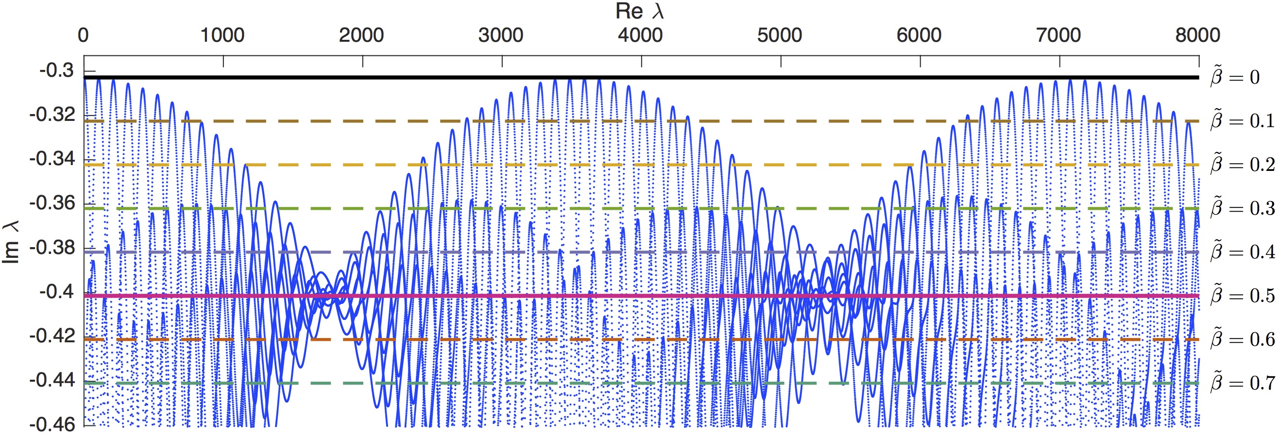
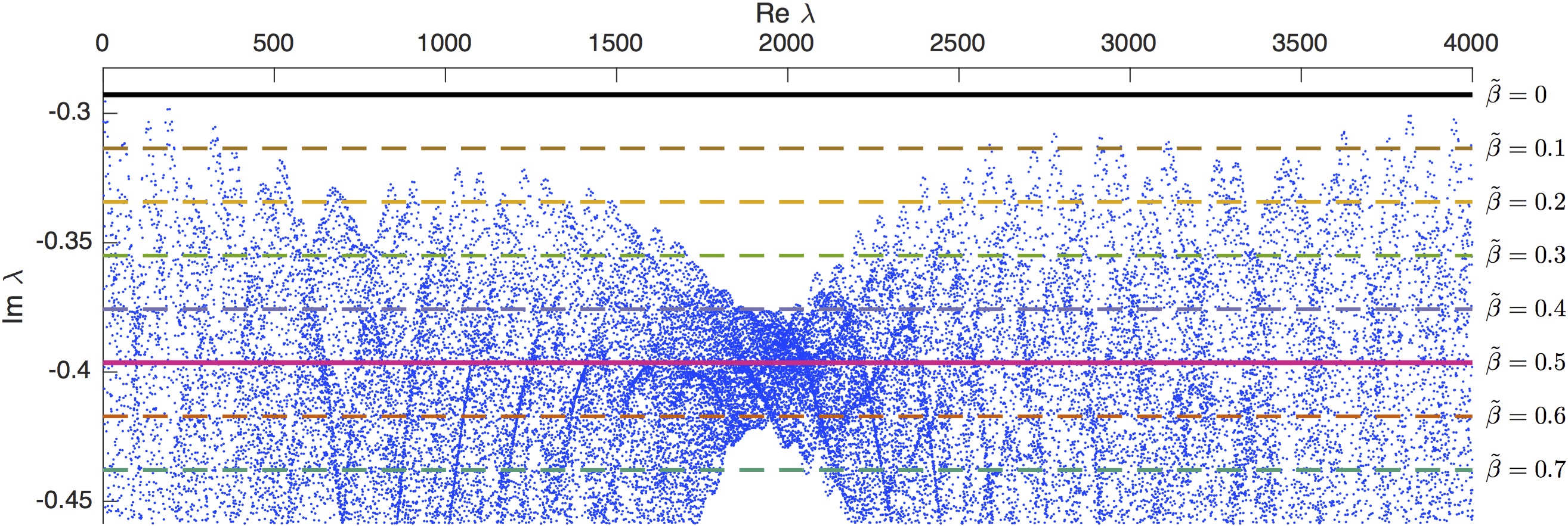
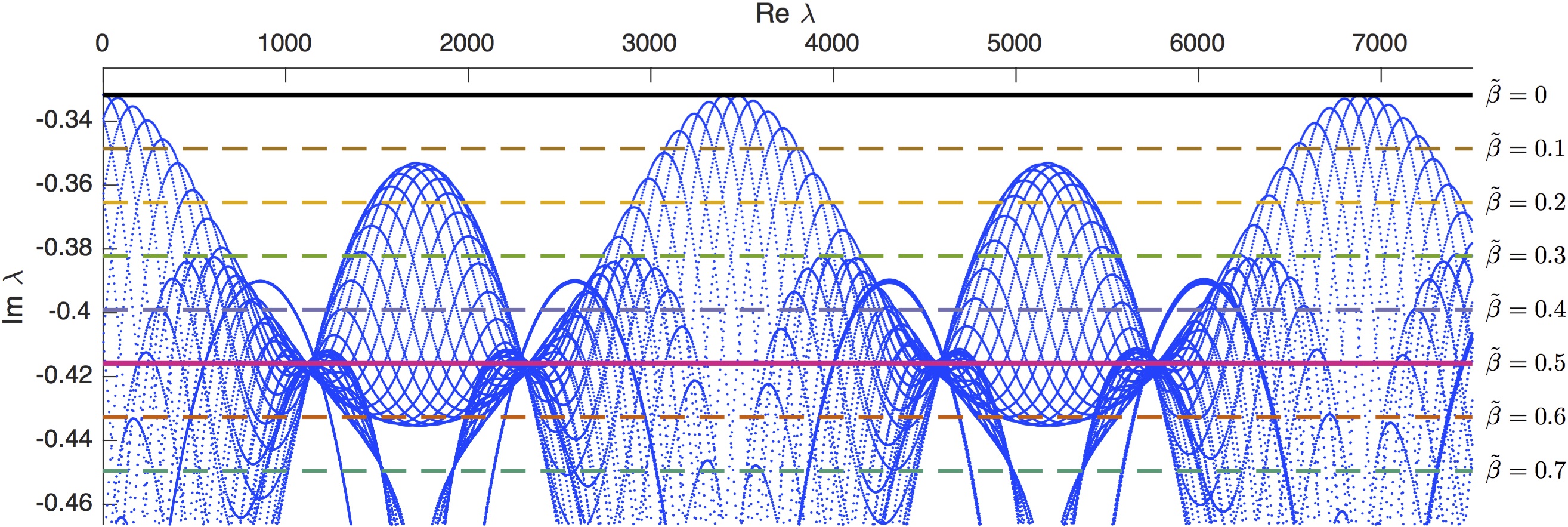
Figure 7. Plot of the numerically calculated resonances for the three-funnel surfaces $X(7,7,7)$ (top), $X(6,7,7)$ (middle) as well as the funneled torus $Y(7,7,\pi/2)$ (bottom). The horizontal lines indicate the strips in which the counting function is analyzed in §A.4. One clearly sees the concentration phenomenon of the resonances at $\tilde{\beta}=0.5$; see (A.2) below for the definition of $\tilde{\beta}$. Additionally one sees alignment of resonances along characteristic chains which have been studied in [WBKPS, BFW, We], as well as concentration of resonance density at $\tilde{\beta}=1/2$ which has been studied in [Bo14, Section 8].

In [Bo14] one of the authors presented an efficient numerical algorithm to calculate the resonances on Schottky surfaces. We refer to [Bo14, BoWe] for details and will only recall the main steps.

The central ingredient for the numerical calculation of resonances on a convex co-compact hyperbolic surface $M=\Gamma\backslash\mathbb{H}^{2}$ is the fact that resonances correspond to zeros of the Selberg zeta function $Z_{\Gamma}(s)$ (1.2). The series expression (1.2) is only absolutely convergent for $\mathrm{Re}(s)>\delta$, thus in the region where no resonances are located. In the region of interest $\mathrm{Re}(s)\leq\delta$, the zeta function is only given by holomorphic continuation, which is not amenable to numerical calculations. One can, however, avoid the problem of holomorphic continuation using a method introduced by Jenkinson–Pollicott [JePo]. These authors use dynamical zeta functions for a transfer operator of the Bowen–Series map, which is an expanding, holomorphic map defined using the generators $g_{i}$

$$\mathcal{B}:\bigcup_{i=1}^{2r}D_{i}\ \to\ \mathbb{C}\cup\{\infty\},$$ (A.1)

where $D_{i}$ are the disks associated to the Schottky group. This transfer operator approach leads to a more efficient series expansion of the zeta function, which converges uniformly on compact sets on the full domain $s\in\mathbb{C}$.

A suitable numerical approximation of the Selberg zeta function on any bounded domain $B\subset\mathbb{C}$ can be obtained by truncating the Jenkinson–Pollicott formula. The zeros can be calculated using efficient adaptive root finding algorithms for holomorphic functions based on the argument principle (see e.g. the algorithm QZ-40 [DSQ]). Figure 7 shows the resulting plots of resonances in the complex plane for the surfaces $X(7,7,7)$, $X(6,7,7)$ and $Y(7,7,\pi/2)$.

In principle, the formulas of Jenkinson–Pollicott can be used to approximate the Selberg zeta function to arbitrary precision on any compact subset of $\mathbb{C}$, simply by including a sufficient number of terms in the truncated series. In practice, however, the complexity of the calculations increases exponentially as additional terms are included. In [BoWe] two of the authors showed that a discrete symmetry group of the surface $M$ leads to a factorization of $Z_{\Gamma}(s)$ into holomorphic symmetry-reduced zeta functions. Using this factorization, the numerical convergence can be dramatically improved. Still, for practical purposes there remain the following restrictions: First, the calculation of resonances becomes dramatically more complicated for higher values of $\delta$. This effectively restricts the calculation of resonances to surfaces with $\delta\lesssim 0.5$. Second, the calculation of $Z_{\Gamma}(1/2-i\lambda)$ becomes exponentially difficult for large negative values of $\operatorname{Im}\lambda$. It is possible to calculate the resonances in a strip of the width of a few deltas parallel to the real axis, but not much beyond this. Third, the calculations also become exponentially complex for high values of $\operatorname{Re}\lambda$. However, here the growth of complexity is several orders of magnitude slower compared to the case of large negative $\operatorname{Im}\lambda$. This allows the computation of counting functions $\mathcal{N}(R,\beta)$ for the surfaces from Figure 7 with $\beta=0.5-0.3\delta$ up to values of $R\approx 10^{5}$.

A.3. Upper bounds on resonance density

We now come to a more detailed examination of resonance densities in strips $\{\operatorname{Im}\lambda\geq-\beta\}$. Let $M$ be a convex co-compact hyperbolic surface and denote by $\operatorname{Res}_{M}$ the set of its resonances. In order to compare results for different surfaces, it is useful to introduce a rescaled parameter

$$\tilde{\beta}:=\frac{\beta-1/2}{\delta}+1,\quad\beta={1\over 2}+(\tilde{\beta}-1)\delta.$$ (A.2)

This has the intuitive interpretation that it gives the width of the resonance counting strip in multiples of $\delta$, with the Patterson–Sullivan gap $\beta={1\over 2}-\delta$ corresponding to $\tilde{\beta}=0$ and the value $\tilde{\beta}=1/2$ corresponds to the spectral gap conjecture of [JaNa12]. Concentration of resonances near the ‘classical decay rate’ line $\{\operatorname{Im}\lambda={\delta-1\over 2}\}$ corresponding to $\tilde{\beta}=1/2$ was first observed (in a different setting) in [LSZ].

For $R,\tilde{\beta}>0$ we introduce the total counting function

$$N(R,\tilde{\beta})=\#\{\lambda\in\operatorname{Res}_{M},\ \operatorname{Re}\lambda\in[0,R],\ \operatorname{Im}\lambda\geq-\beta\},$$

as well as the local counting function (for fixed $L>0$)

$$n(R,\tilde{\beta},L)=\#\{\lambda\in\operatorname{Res}_{M},\ \operatorname{Re}\lambda\in[R,R+L],\ \operatorname{Im}\lambda\geq-\beta\}.$$

In the case of surfaces, Theorem 1 yields an upper bound on

$$n(R,\tilde{\beta},1)=\mathcal{N}(R,1/2+(\tilde{\beta}-1)\delta)$$

Note, however, that the choice $L=1$ in Theorem 1 was made for convenience. The same estimate applies for arbitrary fixed $L>0$, with an adjustment of the constant. Theorem 1 thus implies the bounds

$$N(R,\tilde{\beta}) \leq C_{\tilde{\beta}}R^{1+m(\tilde{\beta},\delta)+\varepsilon},\quad R\to\infty;$$ (A.3)

$$n(R,\tilde{\beta},L) \leq C_{\tilde{\beta},L}R^{m(\tilde{\beta},\delta)+\varepsilon},\quad R\to\infty;$$ (A.4)

$$\text{with}\quad m(\tilde{\beta},\delta) :=\min(2\tilde{\beta}\delta,\delta).$$ (A.5)

As mentioned in the introduction, in the special case of convex co-compact hyperbolic surfaces Naud [Na14] and Jakobson–Naud [JaNa16] previously obtained improved upper bounds on resonance densities which we compare with the bounds of Theorem 1. Using the estimates in [JaNa16], in particular §§4.3,4.4 and Lemma 4.4 there, one can derive an upper bound

$$n(R,\tilde{\beta},L) \leq C_{\beta,L}R^{m_{P}(\tilde{\beta},\delta)+\varepsilon},\quad R\to\infty;$$

$$\text{with }m_{P}(\tilde{\beta},\delta) :=\delta+\min\Big{(}0,{P(2\delta(1-\tilde{\beta}))\over\lambda_{\mathrm{max}}}\Big{)}.$$ (A.6)

In this formula $P(x)$ is the topological pressure of the Bowen–Series map $\mathcal{B}$ (see (A.1)) and $\lambda_{\mathrm{max}}:=\max_{z\in\Lambda_{\Gamma}}\log(\mathcal{B}^{\prime}(z))$ is the maximal Jacobian of $\mathcal{B}$ on the limit set $\Lambda_{\Gamma}$, which coincides with the maximal invariant compact set of the Bowen Series maps.

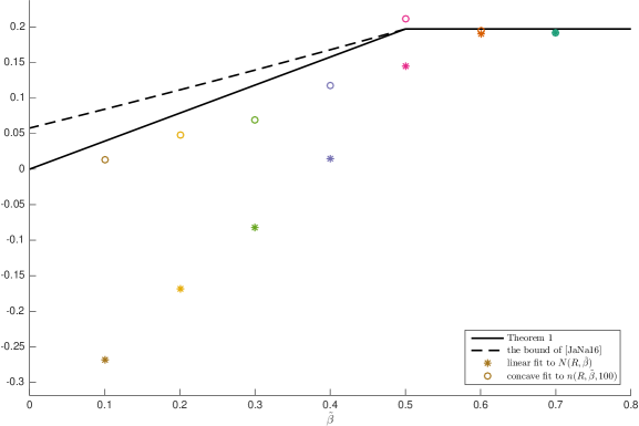
Figure 8. Comparison of the exponents $m_{\mathrm{fit},N}$ (stars) and $m_{\mathrm{mean},n}$ (circles) which have been obtained from the numerical counting function of $X(7,7,7)$. The solid line shows the upper bound $m(\tilde{\beta},\delta)$ from Theorem 1, the dashed line the bound $m_{P}(\tilde{\beta},\delta)$ of [JaNa16]. For $\tilde{\beta}\geq 0.5$, both of these coincide with the previous bound of [GLZ].

In contrast to (A.5), the bound (A.6) depends crucially on the choice of the Schottky marking for a given convex co-compact surface. Independently of the choice of the Schottky marking one however always has the relation

$$m(\tilde{\beta},\delta)\leq m_{P}(\tilde{\beta},\delta).$$ (A.7)

This can be seen as follows: For the Bowen–Series maps the topological pressure function is continuous and monotonically decreasing, and its unique zero is given by $\delta$. Consequently $m(\tilde{\beta},\delta)=m_{P}(\tilde{\beta},\delta)=\delta$ for $\tilde{\beta}\geq 1/2$. Additionally one knows that $P^{\prime}(x)\geq-\lambda_{\mathrm{max}}$ and consequently

$$\frac{d}{d\tilde{\beta}}m_{P}(\tilde{\beta},\delta)\ \leq\ 2\delta=\frac{d}{d\tilde{\beta}}m(\tilde{\beta},\delta).$$

for $0\leq\tilde{\beta}<1/2$ which implies (A.7).

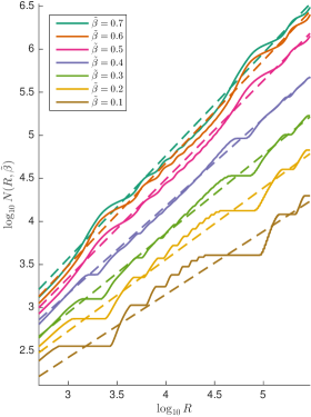
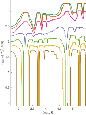
Figure 9. Double logarithmic plot of the total counting function (left) and local counting function (right; see (A.9)) for the three-funnel surface $X(7,7,7)$ and different values of $\tilde{\beta}$. The dashed lines in the left plot indicate linear fits to the double logarithmic data points, see (A.8).

In Figures 8, 13, and 13 below we compare the two bounds for three different convex co-compact surfaces. For this purpose the topological pressure has been numerically calculated according to [JePo]. One clearly sees that in all cases (A.7) holds. While the difference is rather pronounced for both three-funnel examples, the difference for the funneled torus is relatively small. The expansion rate of the Bowen–Series map for the funneled torus is much more homogeneous than for the two other examples. This observation therefore suggests that the two bounds become close to each other for surfaces that admit a very homogeneous Bowen–Series map.

A.4. Comparison of theoretical upper bounds with numerics

Let us now compare the upper bounds to numerical calculations of the counting function. Using the approach described in §A.2, we calculated $N(R,\tilde{\beta})$ for the surface $X(7,7,7)$ with $\tilde{\beta}=0.1,0.2,\ldots,0.7$ and $R=100,200,\ldots,3\cdot 10^{5}$. Note that it is not necessary to calculate the exact position of the resonances, since the argument principle directly allows to calculate the number of zeros of $Z_{\Gamma}(s)$ in rectangular boxes.

A log-log plot of the total counting function is presented in the left part of Figure 9. We observe that the counting functions behave approximately linearly, with slopes that clearly decrease with decreasing $\tilde{\beta}$. All counting functions also show clearly visible oscillations, which we assume to be due to the fact that we are still in a finite-frequency regime. Already in the context of spectral gaps oscillations in the resonance pattern have been observed to be persistent up to very high frequencies (see [BoWe, Figure 13]). For smaller values of $\tilde{\beta}$, i.e. for more narrow strips, these oscillations in the counting function become more pronounced.

We perform a linear regression to the double logarithmic data

$$\log(N(R,\tilde{\beta}))\approx(1+m_{\mathrm{fit},N})\cdot\log(R)+C,$$ (A.8)

where $m_{\mathrm{fit},N},C\in\mathbb{R}$ are chosen to minimize the sum of squares of the difference between the left- and right-hand sides of (A.8) over all data points $R=500,600,\dots,3\cdot 10^{5}$. By this we extract an exponent $m_{\mathrm{fit},N}$ for every value of $\tilde{\beta}$, and compare it to the theoretical upper bound. The parametric dependence of $m_{\mathrm{fit},N}$ on $\tilde{\beta}$ is shown in Figure 8 by the star shaped symbols. One clearly sees that the data points for large $\tilde{\beta}$ (i.e., $\tilde{\beta}>0.5$) agree very well with the theoretical bound. For smaller values of $\tilde{\beta}$ the numerical values are clearly below the upper bound, but there are rather large deviations. In particular we obtain significantly negative values for $m_{\textup{fit},N}$ which implies sublinear growth of the total counting function. It would be interesting to understand whether this is only due to the restricted frequency range or a phenomenon that can be rigorousely understood.

Let us next turn to the behavior of the local counting functions. The right part of Figure 9 shows a double logarithmic plot of $n(R,\tilde{\beta},100)$ for the surface $X(7,7,7)$ and for different values of $\tilde{\beta}$. Since this function oscillates very rapidly (see Figure 10), we instead plot the mollified expression

$$R\ \mapsto\ \max\{\log_{10}n(R^{\prime},\tilde{\beta},100)\colon|\log_{10}(R/R^{\prime})|\leq 0.05\}.$$ (A.9)

We have chosen $L=100$ as we want $L\ll R_{\mathrm{max}}=3\cdot 10^{5}$ on the one hand, but on the other hand we want $L$ to be large relative to the resonance spacing on the chains, which is on the order of $1$. Once again, for different values of $\tilde{\beta}$ one observes clear distinctions in the growth behavior of $\log(n(R,\tilde{\beta},100))$. However, the most prominent features are the strong oscillations of the local counting functions. In particular, for the lower values of $\tilde{\beta}$, i.e., for the narrower strips, there are large $R$-ranges devoid of resonances.

Note, however, that even an optimal asymptotic upper bound for $n(R,\tilde{\beta},L)$ would not exclude large resonance free ranges in narrow strips along the real axis. Rather it would imply that there is no better upper bound for those frequency ranges where the resonances accumulate in the strips. It would thus not be appropriate to extract a numerical exponent for the upper bound by a linear fit of the double logarithmic plot. Instead, we want a method that extracts the mean growth rate of the regions with a high resonance density.

We therefore chose the following two-step method for the extraction of the exponent (see Figure 10):

• first, we construct the concave envelope $n_{\mathrm{concave}}(x)$ of the local counting function, which is the pointwise infimum of all affine functions $x\mapsto ax+b$ which bound the local counting function on the logarithmic scale:

  $$\max(0,\log_{10}n(R,\tilde{\beta},L))\leq a\log_{10}R+b,\quad R=500,600,\dots,3\cdot 10^{5};$$

The resulting concave envelope can be seen as the dashed line in Figure 10. It can be seen, that this concave envelope still contains boundary effects. For example, the end of the calculated data range happened to be in a region where $n(r,\tilde{\beta},100)$ takes very low values, thus the envelope function decays at the end of the data range. This is obviously an artefact occuring at the boundaries of the finite data range. In order to get rid of these effects we perform the

• second step: we define the concave envelope fit $m_{\mathrm{mean},n}$ as the slope of the straight line crossing the graph of $n_{\mathrm{concave}}(x)$ at $x=x_{1},x_{2}$, where $x_{1},x_{2}$ are the points marking $1\over 4$ and $3\over 4$ of the length in the interval $[\log_{10}(500),\log_{10}(3\cdot 10^{5})]$.

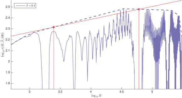
Figure 10. An illustration of the concave fitting procedure for the surface $X(7,7,7)$ and $\tilde{\beta}=0.4$. The rapidly oscillating curve is the logarithmic plot of the local counting function $n(R,\tilde{\beta},100)$. The dashed line is the concave envelope $n_{\mathrm{concave}}(x)$, and the red line is the secant line of the concave envelope used to determine the fit $m_{\mathrm{mean},n}$.

The $\tilde{\beta}$ dependence of the quantity $m_{\mathrm{mean},n}$ is plotted in Figure 8 by the circular symbols. For large $\tilde{\beta}$ (i.e., $\tilde{\beta}>0.5$) the exponents extracted by the total counting function and those extracted from the local counting function agree well with each other and also with the theoretical upper bound. For lower values of $\tilde{\beta}$, the exponents $m_{\mathrm{mean},n}$ are significantly larger and quite close to the theoretical upper bounds. In view of the strong oscillations of $n(R,\tilde{\beta},L)$ this is very plausible. Fitting the log-log data of the total counting function to a linear function implies averaging over the oscillations of the local counting function. The exponent $m_{\mathrm{fit},N}$ thus also incorporates information of the large ranges where the local counting function is small, whereas Theorem 1 gives an upper bound on the asymptotic behavior of the maxima.

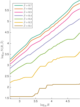
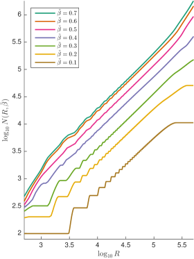
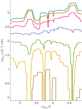
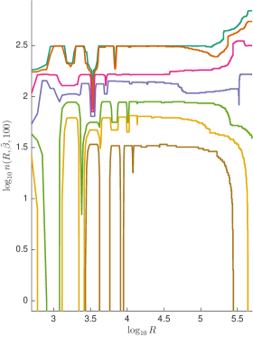
Figure 11. Double logarithmic plot of the total counting function (top) and local counting function (bottom) for the three-funnel surface $X(6,7,7)$ (left) and the funneled torus $Y(7,7,\pi/2)$ (right), similar to Figure 9. Both data sets only represent the resonances corresponding to the trivial representation of the discrete symmetry groups.

Let us finally have a look at two less symmetric surfaces, the three-funnel surface $X(6,7,7)$ and the funneled torus $Y(7,7,\pi/2)$. As these surfaces have a much smaller symmetry group compared to the completely symmetric surface $X(7,7,7)$, the calculations at high frequencies are much more time-consuming. We therefore restricted the calculation of the counting function to those resonances that belong to the trivial representation of the discrete symmetry group (c.f. [BoWe]). Figure 11 shows double logarithmic plots of the total counting function as well as the local counting function. Similarly to the surface $X(7,7,7)$ both counting functions show oscillating behavior. In particular, for the funneled torus one sees a visible kink in the counting function right before the end of the numerically accessible range, which indicates that one might need to go to significantly higher frequencies to see the full asymptotic behavior.

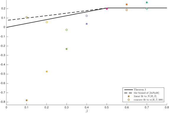
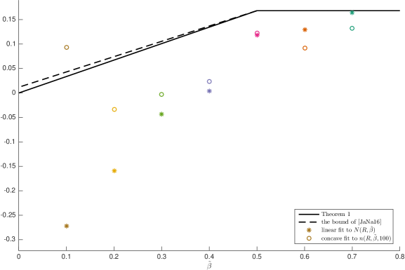
Figure 12. Same as Figure 8 but for the surface $X(6,7,7)$.

Figure 13. Same as Figure 8 but for the surface $Y(7,7,\pi/2)$.

By the same procedures as above we extract the exponents $m_{\mathrm{fit},N}$ and $m_{\mathrm{mean},n}$ from the numerical data. The $\tilde{\beta}$ dependence and a comparison with the prediction of Theorem 1 are shown in Figures 13 and 13. Both figures show again that the coincidence of the numerical exponent with the upper bounds is rather good for $\tilde{\beta}>0.5$. For lower $\tilde{\beta}$ values the exponents extracted from the concave upper bound are slightly below the upper bound of Theorem 1. Only for the most narrow band with $\tilde{\beta}=0.1$ is the mean exponent above this bound. However in these narrow strips there are huge resonance-free frequency ranges. Thus the counting functions have a rather poor statistic, such that the extracted exponents have to be taken with caution. Comparing Figures 13 and 13, one sees that the exponents for the funneled torus are much less coherent. We attribute this to the kink described above, and assume that the data would be more conclusive if one could go to significantly higher frequency ranges.

In summary, we have compared the numerical data to the theoretical upper bound. Using the concave average method we were able to extract exponents which describe an asymptotic upper bound for the local counting function. The numerical results suggest that while the upper bound from Theorem 1 is not completely optimal, it seems not to be far off for the surfaces studied. In particular, for $X(7,7,7)$ (Figure 8), where the high symmetry allows the most exhaustive numerical calculations (in particular we were able to calculate the spectrum of all symmetry classes) and which we can thus consider to be the most reliable case, the exponents $m_{\mathrm{mean},n}$ are close to the theoretical predictions.

Acknowledgements. The authors would like to thank Maciej Zworski, Long Jin, Stéphane Nonnenmacher, Kiril Datchev, and Colin Guillarmou for many useful discussions regarding this project, and Frédéric Naud for several discussions of [Na14, JaNa16], in particular explaining the bound (A.6). We would also like to thank two anonymous referees for many useful comments to improve the paper. This research was conducted during the period SD served as a Clay Research Fellow. TW has been supported by the grant DFG HI 412 12-1.

References

• [BFW] Sonja Barkhofen, Frédéric Faure, and Tobias Weich, Resonance chains in open systems, generalized zeta functions and clustering of the length spectrum, Nonlinearity 27(2014), 1829–1858.
• [BWPSKZ] Sonja Barkhofen, Tobias Weich, Alexander Potzuweit, Hans-Jürgen Stöckmann, Ulrich Kuhl, and Maciej Zworski, Experimental observation of the spectral gap in microwave $n$-disk systems, Phys. Rev. Lett. 110(2013), 164102.
• [Bo16] David Borthwick, Spectral theory of infinite-area hyperbolic surfaces, second edition, Birkhäuser, 2016.
• [Bo14] David Borthwick, Distribution of resonances for hyperbolic surfaces, Experimental Math. 23(2014), 25–45.
• [BoWe] David Borthwick and Tobias Weich, Symmetry reduction of holomorphic iterated function schemes and factorization of Selberg zeta functions, to appear in J. Spect. Th., arXiv:1407.6134.
• [Bu] Jack Button, All Fuchsian Schottky groups are classical Schottky groups, The Epstein birthday Schrift – Geom. Topol. Publ. 117–125 (1998).
• [DaDy] Kiril Datchev and Semyon Dyatlov, Fractal Weyl laws for asymptotically hyperbolic manifolds, Geom. Funct. Anal. 23(2013), 1145–1206.
• [DSQ] Michael Dellnitz, Oliver Schütze, and Qinghua Zheng, Locating all the zeros of an analytic function in one complex variable, J. Comp. Appl. Math.138(2)(2002), 325–333.
• [Dy] Semyon Dyatlov, Resonance projectors and asymptotics for $r$-normally hyperbolic trapped sets, J. Amer. Math. Soc. 28(2015), 311–381.
• [DyJi16] Semyon Dyatlov and Long Jin, Resonances for open quantum maps and a fractal uncertainty principle, to appear in Comm. Math. Phys., arXiv:1608.02238.
• [DyWa] Semyon Dyatlov and Alden Waters, Lower resolvent bounds and Lyapunov exponents, Appl. Math. Res. Expr. 2016, 68–97.
• [DyZa] Semyon Dyatlov and Joshua Zahl, Spectral gaps, additive energy, and a fractal uncertainty principle, Geom. Funct. Anal. 26(2016), 1011–1094.
• [DyZw] Semyon Dyatlov and Maciej Zworski, Mathematical theory of scattering resonances, book in progress, http://math.mit.edu/~dyatlov/res/
• [GoSi] Israel C. Gohberg and Efim I. Sigal, An operator generalization of the logarithmic residue theorem and Rouché’s Theorem, Mat. Sb. 84(126)(1971), 607–629.
• [Gu] Colin Guillarmou, Meromorphic properties of the resolvent on asymptotically hyperbolic manifolds, Duke Math. J. 129:1(2005), 1–37.
• [GLZ] Laurent Guillopé, Kevin K. Lin, and Maciej Zworski, The Selberg zeta function for convex co-compact Schottky groups, Comm. Math. Phys. 245:1(2004), 149–176.
• [GuZw95] Laurent Guillopé and Maciej Zworski, Polynomial bounds on the number of resonances for some complete spaces of constant negative curvature near infinity, Asymptotic Anal. 11:1(1995), 1–22.
• [GuZw99] Laurent Guillopé and Maciej Zworski, The wave trace for Riemann surfaces, Geom. Funct. Anal. 9(1999), 1156–1168.
• [JaNa12] Dmitry Jakobson and Frédéric Naud, On the critical line of convex co-compact hyperbolic surfaces, Geom. Funct. Anal. 22(2012), 352–368.
• [JaNa16] Dmitry Jakobson and Frédéric Naud, Resonances and density bounds for convex co-compact congruence subgroups of $\operatorname{SL}_{2}(\mathbb{Z})$, Israel J. Math. 213(2016), 443–473.
• [JePo] Oliver Jenkinson and Mark Pollicott, Calculating Hausdorff dimension of Julia sets and Kleinian limit sets, Amer. J. Math. 124(2002), 495–545.
• [LSZ] Wentao Lu, Srinivas Sridhar, and Maciej Zworski, Fractal Weyl laws for chaotic open systems, Phys. Rev. Lett. 91(2003), 154101.
• [MaMe] Rafe Mazzeo and Richard Melrose, Meromorphic extension of the resolvent on complete spaces with asymptotically constant negative curvature, J. Funct. Anal. 75(1987), 260–310.
• [Na05] Frédéric Naud, Expanding maps on Cantor sets and analytic continuation of zeta functions, Ann. de l’ENS (4) 38(2005), 116–153.
• [Na14] Frédéric Naud, Density and location of resonances for convex co-compact hyperbolic surfaces, Invent. Math. 195(2014), 723–750.
• [Non] Stéphane Nonnenmacher, Spectral problems in open quantum chaos, Nonlinearity 24(2011), R123.
• [NoZw] Stéphane Nonnenmacher and Maciej Zworski, Decay of correlations for normally hyperbolic trapping, Invent. Math. 200(2015), 345–438.
• [Nov] Marcel Novaes, Supersharp resonances in chaotic wave scattering, Phys. Rev. E 85(2012), 036202.
• [Pa] Samuel James Patterson, The limit set of a Fuchsian group, Acta Math. 136(1976), 241–273.
• [Pe87] Peter Perry, The Laplace operator on a hyperbolic manifold I. Spectral and scattering theory, J. Funct. Anal. 75(1987), 161–187.
• [Pe03] Peter Perry, A Poisson summation formula and lower bounds for resonances in hyperbolic manifolds, Int. Math. Res. Not. 34(2003), 1837–1851.
• [PWBKSZ] Alexander Potzuweit, Tobias Weich, Sonja Barkhofen, Ulrich Kuhl, Hans-Jürgen Stöckmann, and Maciej Zworski, Weyl asymptotics: from closed to open systems, Phys. Rev. E. 86(2012), 066205.
• [Sh] Dmitry Shepelyanski, Fractal Weyl law for quantum fractal eigenstates, Phys. Rev. E 77(2008), 015202.
• [Sj] Johannes Sjöstrand, Geometric bounds on the density of resonances for semiclassical problems, Duke Math. J. 60:1(1990), 1–57.
• [SjZw] Johannes Sjöstrand and Maciej Zworski, Fractal upper bounds on the density of semiclassical resonances, Duke Math. J. 137(2007), 381–459.
• [St] Luchezar Stoyanov, Spectra of Ruelle transfer operators for axiom A flows, Nonlinearity 24(2011), 1089–1120.
• [Su] Dennis Sullivan, The density at infinity of a discrete group of hyperbolic motions, Publ. Math. de l’IHES 50(1979), 171–202.
• [Va1] András Vasy, Microlocal analysis of asymptotically hyperbolic and Kerr–de Sitter spaces, with an appendix by Semyon Dyatlov, Invent. Math. 194(2013), 381–513.
• [Va2] András Vasy, Microlocal analysis of asymptotically hyperbolic spaces and high energy resolvent estimates, Inverse Problems and Applications. Inside Out II, Gunther Uhlmann (ed.), MSRI publications 60, Cambridge Univ. Press, 2013.
• [We] Tobias Weich, Resonance chains and geometric limits on Schottky surfaces, Comm. Math. Phys. 337(2015), 727–765.
• [WBKPS] Tobias Weich, Sonja Barkhofen, Ulrich Kuhl, Charles Poli, and Henning Schomerus, Formation and interaction of resonance chains in the open 3-disk system, New Journal of Physics 16(2014), 033029.
• [Zw99] Maciej Zworski, Dimension of the limit set and the density of resonances for convex co-compact hyperbolic surfaces, Invent. Math. 136(1999), 353–409.
• [Zw12] Maciej Zworski, Semiclassical analysis, Graduate Studies in Mathematics 138, AMS, 2012.
• [Zw16] Maciej Zworski, Resonances for asymptotically hyperbolic manifolds: Vasy’s method revisited, J. Spect. Th. 6(2016), 1087–1114.