Hyperon elastic electromagnetic form factors in the space-like momentum region

Abstract

We present a calculation of the electric and magnetic form factors of ground-state octet and decuplet baryons including strange quarks. We work with a combination of Dyson-Schwinger equations for the quark propagator and covariant Bethe-Salpeter equations describing baryons as bound states of three (non-perturbative) quarks. Our form factors for the octet baryons are in good agreement with corresponding lattice data at finite $Q^{2}$; deviations in some isospin channels for the magnetic moments can be explained by missing meson cloud effects. At larger $Q^{2}$ our quark core calculation has predictive power for both, the octet and decuplet baryons.

1 Introduction

The composite structure of hadronic bound states is encoded in their form factors. While there is abundant experimental information on the nucleon electromagnetic structure Burkert:2004sk ; Pascalutsa:2006up , our experimental knowledge of the structure of other baryons and, in particular, of those with strange-quark content (hyperons) is scarce and limited to some values for static properties Agashe:2014kda ; GoughEschrich:2001ji ; Taylor:2005zw ; Keller:2011aw ; Keller:2011nt . First measurements of hyperon form factors at large time-like photon momentum have been presented recently by the CLEO collaboration Dobbs:2014ifa . The study of the hyperon structure is also one of the main goals of the CLAS collaboration.

On the theoretical side, there have been many attempts to shed light on the issue of the electromagnetic structure of octet and decuplet baryons. Model calculations using bag models Umino:1991dk , quark models Darewych:1983yw ; Kaxiras:1985zv ; Sahoo:1995kg ; Sharma:2010vv ; Wagner:1995va ; Wagner:1998bu ; Wagner:1998fi ; Wagner:2000ii ; Buchmann:2002xq ; VanCauteren:2003hn ; VanCauteren:2005sm ; VanCauteren:2005vr ; Metsch:2008zz , instanton models Merten:2002nz , QCD sum rules Liu:2009mb ; Aliev:2013jda ; Aliev:2013jta ; Aliev:2013mda , Skyrme models Scoccola:1999ke , chiral perturbation theory Kubis:2000aa ; Arndt:2003vd ; Wang:2008vb and covariant spectator models Ramalho:2009vc ; Ramalho:2010xj ; Ramalho:2011pp ; Ramalho:2012ad ; Ramalho:2012im ; Ramalho:2012pu ; Ramalho:2013iaa ; Ramalho:2013uza , show a varying degree of success. A coherent microscopic description of strong and electromagnetic baryon form factors has therefore not yet emerged. Lattice QCD Leinweber:1990dv ; Leinweber:1992hy ; Leinweber:1992pv ; Boinepalli:2006xd ; Lin:2007gv ; Boinepalli:2009sq ; Shanahan:2014uka ; Shanahan:2014cga is progressively overcoming its limitations and starting to provide more precise ab initio data. While for the octet hyperons these already complement experimental knowledge, corresponding results for decuplet hyperons are only available for some static observables and are still plagued with huge uncertainties.

In this work we use the combination of Dyson-Schwinger (DSE) and covariant Bethe-Salpeter (BSE) equations to study the elastic electromagnetic form factors of ground-state spin-$\nicefrac{{1}}{{2}}$ and spin-$\nicefrac{{3}}{{2}}$ hyperons. The combined framework of DSEs and BSEs provides a rigorously defined connection between QCD as a quantum field theory and hadronic observables. The dynamics of quarks and gluons as constituents of bound states, as well as the interaction vertices among them, is determined by the infinite set of coupled DSEs; these are the necessary elements to define the relevant BSEs, from which solutions one obtains all the properties of hadrons as bound states of quarks and gluons. In practice, for most applications the infinite tower of DSEs must be truncated into a finite number of equations. The truncation on the DSEs is non-trivially related to the truncation on the BSEs, such that all the relevant symmetries are preserved; see, e.g. Sanchis-Alepuz:2015tha for a review of the formalism.

The leading-order truncation of the DSE/BSE system is the so-called rainbow-ladder (RL) truncation, which is able to reproduce fairly well many hadron observables (a selection of results can be found in Eichmann:2013afa and references therein). In particular, a series of recent works Eichmann:2009qa ; Eichmann:2011vu ; Eichmann:2011pv ; SanchisAlepuz:2011jn ; Sanchis-Alepuz:2013iia ; Alkofer:2014bya ; Sanchis-Alepuz:2014sca ; Sanchis-Alepuz:2014wea have focused on providing a description of ground-state baryons as three-quark objects in the RL truncation. This work adds to this effort by completing the study of space-like elastic electromagnetic properties of the baryon octet and decuplet ground states.

This paper is organised as follows. In section 2 we review the basic elements of the DSE/BSE formalism. In section 3 we discuss the assets and limitations of the RL scheme and present and discuss results for the electromagnetic properties of octet and decuplet hyperons. We summarise and conclude in section 4. In several appendices we collect technical details of the framework.

2 Review of the formalism

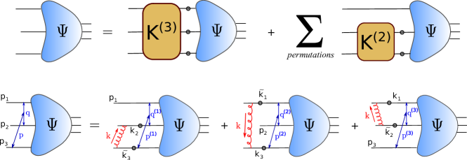
Figure 1: Upper figure: Diagrammatic representation of the three-body Bethe-Salpeter equation with amplitude $\Psi$. Full quark propagators are denoted by straight lines with black dots. The interaction between the quarks are encoded in the three-body and two-body kernels $K^{(3)}$ and $K^{(2)}$. Lower figure: Faddeev equation in the rainbow-ladder truncation; see Appendix D for the definitions of momenta.

In the Bethe-Salpeter framework, a baryon is described by the three-body Bethe-Salpeter amplitude $\Gamma_{ABCD}(p_{1},p_{2},p_{3})$, where we use $\{ABC\}$ as generic indices for spin, flavour and colour indices (e.g. $A\rightarrow\{\alpha,a,r\}$, respectively) for the valence quarks and similarly we use $D$ as a collective index for the resulting baryon. This amplitude is the solution of the three-body Bethe-Salpeter equation Fig. 1. The amplitude depends on the three quark momenta $p_{1,2,3}$, which can be expressed in terms of two relative momenta $p$ and $q$ and the total momentum $P$ (see Eq. (D) in Appendix D). It is decomposed in a tensor product of a spin-momentum part to be determined and flavour and colour parts which are fixed

$$\Gamma_{ABCD}(p,q,P)=\left(\sum_{\rho}\Psi^{\rho}_{\alpha\beta\gamma\mathcal{I}}(p,q,P)\otimes F^{\rho}_{abcd}\right)\otimes\frac{\epsilon_{rst}}{\sqrt{6}}~{}.$$ (1)

The colour term $\epsilon_{rst}/\sqrt{6}$ fixes the baryon to be a colour singlet and the flavour terms $F^{\rho}_{abcd}$ are the quark-model $SU(3)$-symmetric and mixed representations (see Sanchis-Alepuz:2014sca ). The index $\rho$ denotes the representation of the $SU(3)$ group to which the baryon belongs (mixed-symmetric or mixed-antisymmetric representation for the baryon octet and symmetric representation for the baryon decuplet).

The spin-momentum part of the Bethe-Salpeter amplitude, $\Psi^{\rho}_{\alpha\beta\gamma\mathcal{I}}(p,q,P)$, is a tensor with three Dirac indices $\alpha,\beta,\gamma$ associated to the valence quarks and a generic index $\mathcal{I}$ whose nature depend on the spin of the resulting bound state. They can in turn be expanded in a covariant basis $\{\tau(p,q;P)\}$

$$\Psi^{\rho}_{\alpha\beta\gamma\mathcal{I}}(p,q,P)=f^{\rho}_{i}(p^{2},q^{2},z_{0},z_{1},z_{2})\tau_{\alpha\beta\gamma\mathcal{I}}^{i}(p,q;P)~{},$$ (2)

where the scalar coefficients $\{f\}$ depend on Lorentz scalars $p^{2}$, $q^{2}$, $z_{0}=\widehat{p_{T}}\cdot\widehat{q_{T}}$, $z_{1}=\widehat{p}\cdot\widehat{P}$ and $z_{2}=\widehat{q}\cdot\widehat{P}$ only. The subscript $T$ denotes transverse projection with respect to the total momentum and vectors with hat are normalised. A covariant basis can be obtained using symmetry requirements only; for positive-parity spin-$\nicefrac{{1}}{{2}}$ baryons it contains 64 elements Eichmann:2009en ; Eichmann:2009zx whereas for spin-$\nicefrac{{3}}{{2}}$ baryons it contains 128 elements SanchisAlepuz:2011jn . In this way, one only needs to solve for the scalar functions $f$.

To define the three-body BSE, Fig. 1, one needs to specify the three-particle and two-particle irreducible kernels, $K^{(3)}$ and $K^{(2)}$, respectively. In the Faddeev approximation the three-body irreducible interactions are neglected, and we refer to the simplified BSE as the Faddeev equation (FE). In addition one needs to know the full quark propagator $S$ (omitting now Dirac indices) for the quark flavours of interest. In general it can be written as

$$S^{-1}(p)=A(p^{2})\left(i\ooalign{\hfil/\hfil\crcr$p$}+B(p^{2})/A(p^{2})\right)~{},$$ (3)

with vector and scalar dressing functions $A(p^{2})$ and $B(p^{2})$. The ratio $M(p^{2})=B(p^{2})/A(p^{2})$ is a renormalisation group invariant and describes the running of the quark mass with momentum. The dressing functions are obtained as solutions of the quark DSE

$$S^{-1}(p)=S^{-1}_{0}(p)+Z_{1f}g^{2}C_{F}\!\!\int_{q}\!\gamma^{\mu}D_{\mu\nu}(p-q)\Gamma^{\nu}(p,q)S(q)\,\,,$$ (4)

which also contains the full quark-gluon vertex $\Gamma^{\nu}$ and the full gluon propagator $D_{\mu\nu}$; $S_{0}$ is the (renormalised) bare propagator with inverse

$$S_{0}^{-1}(p)=Z_{2}\left(i\ooalign{\hfil/\hfil\crcr$p$}+m\right)\,,$$ (5)

where $m$ is the bare quark mass and $Z_{1f}$ and $Z_{2}$ are renormalisation constants. The renormalised strong coupling is denoted by $g$ and $\int_{q}=\int\frac{d^{4}q}{(2\pi)^{4}}$ abbreviates a four-dimensional integral in momentum space supplemented with a translationally invariant regularisation scheme.

Under certain symmetry requirements, the practical solution of the Faddeev equation can be greatly simplified by relating the three two-body interaction diagrams in Fig. 1. As shown in Eichmann:2011vu ; Sanchis-Alepuz:2014sca , taking the flavour part of the Faddeev amplitudes as representations of the $SU(3)$ group induces a specific transformation rule for the spin-momentum part under interchange of its valence-quark indices. In this case the Faddeev equation for the coefficients $f$ reduces to

$$f^{\rho}_{i}(p^{2},q^{2},z_{0},z_{1},z_{2})=$$

$$C\mathcal{F}_{1}^{\rho\rho^{\prime};\lambda}~{}H_{1}^{ij} ~{}g^{\rho^{\prime\prime},\lambda}_{j}(p^{\prime 2},q^{\prime 2},z^{\prime}_{0},z^{\prime}_{1},z^{\prime}_{2})+$$

$$C\mathcal{F}_{2}^{\rho\rho^{\prime};\lambda}~{}H_{2}^{ij} ~{}g^{\rho^{\prime\prime},\lambda}_{j}(p^{\prime\prime 2},q^{\prime\prime 2},z^{\prime\prime}_{0},z^{\prime\prime}_{1},z^{\prime\prime}_{2})+$$

$$C\mathcal{F}_{3}^{\rho\rho^{\prime};\lambda}~{} ~{}g^{\rho^{\prime},\lambda}_{i}(p^{2},q^{2},z_{0},z_{1},z_{2})~{},$$ (6)

with the colour factor $C=-\nicefrac{{2}}{{3}}$ and the flavour matrices $\mathcal{F}$, the rotation matrices $H$ and other symbols defined in Appendix D (see also Sanchis-Alepuz:2014sca ). Here, the index $\lambda$ runs over all elements in a given flavour state (e.g. $\lambda=1,2$ for the mixed-symmetric flavour wave function of the proton and $\lambda=1,3$ for the mixed-antisymmetric one; see Appendix C). With this simplification, one needs to solve for one of the diagrams only. For example, particularly simple to solve numerically is

$$g^{\rho,\lambda}_{i}(p^{2},q^{2},z_{0},z_{1},z_{2})=$$

$$\int_{k}~{}\textnormal{Tr}\Bigl{[}~{}\bar{\tau}^{i}_{\beta\alpha\mathcal{I}\gamma}(p,q,P) K_{\alpha\alpha^{\prime},\beta\beta^{\prime}}(p,q,k)\delta_{\gamma\gamma^{\prime\prime}}\times$$

$$S^{(\lambda_{1})}_{\alpha^{\prime}\alpha^{\prime\prime}}(k_{1})S^{(\lambda_{2})}_{\beta^{\prime}\beta^{\prime\prime}} (k_{2})~{}\tau^{j}_{\alpha^{\prime\prime}\beta^{\prime\prime}\gamma^{\prime\prime}\mathcal{I}}(p_{(3)},q_{(3)},P)~{}\Bigr{]}\times$$

$$f^{\rho}_{j}(p_{(3)}^{2},q_{(3)}^{2},z^{(3)}_{0},z^{(3)}_{1},z^{(3)}_{2})~{}.$$ (7)

where now the quark at the position $\ell$ in each term of the flavour wave function is denoted by the superindex $\lambda_{\ell}$ to keep track of the different flavours. The internal relative momenta $p_{(3)}$, $q_{(3)}$ (and analogously for $z^{(3)}_{0}$, $z^{(3)}_{1}$ and $z^{(3)}_{2}$) are defined in Appendix D. The conjugate of the covariant basis $\bar{\tau}$ has been defined in Eichmann:2009en ; SanchisAlepuz:2011jn and it is assumed that the basis $\{\tau\}$ is orthonormal.

These considerations are valid for rather general interaction kernels. However, in general the kernel contains all possible two-body irreducible interactions among quarks and for any practical implementation of Eq. (2) one must truncate it. The BSEs kernels can be related to the integration kernel in the quark DSE via functional derivatives Fukuda:1987su ; McKay:1989rk ; Munczek:1994zz ; Sanchis-Alepuz:2015tha . Specifically, if the theory is defined via an nPI effective action, a loop expansion of the action translates into a truncation of the DSE/BSE system. Moreover, if the truncation is defined in this way, the requirements of chiral symmetry expressed by axial-vector and vector Ward-Takahashi identities leading to massless pions in the chiral limit from the pseudo-scalar meson BSE are automatically fulfilled. In such a scheme, the leading truncation corresponds to the case in which the full gluon propagator and full quark-gluon vertex in (4) are truncated to their tree-level part, and the corresponding two-body kernel is a single-gluon exchange with a tree-level vector-vector coupling to quarks. In order to generate dynamical chiral-symmetry breaking and be able to reproduce hadron phenomenology, the interaction is infrared-enhanced with an effective coupling $\alpha_{\textrm{eff}}$ which has to be modelled (see sect. 2.2). This is the rainbow-ladder truncation of the DSE/BSE system. Its salient features are simplicity, while maintaining the correct momentum running of the quark propagator and the underlying quark-gluon interaction in the medium to large momentum region. Efforts to improve upon the rainbow-ladder scheme can be found e.g. in Refs. Bender:1996bb ; Watson:2004kd ; Bhagwat:2004hn ; Matevosyan:2006bk ; Fischer:2009jm ; Chang:2009zb ; Heupel:2014ina ; Fischer:2007ze ; Sanchis-Alepuz:2014wea . We will discuss the assets and limitations of the rainbow-ladder approach below in section 3.

2.1 Form factor calculation in the BSE approach

The procedure to couple an external field to a BSE equation is called gauging of the equation and was introduced in Haberzettl:1997jg ; Kvinikhidze:1998xn ; Kvinikhidze:1999xp . The main features of this procedure is that it ensures gauge invariance in the coupling with an external electromagnetic field (hence charge conservation) and prevents the over-counting of diagrams. The specific application of this formalism in the RL-truncated three-body BSE framework has been already described in Eichmann:2011vu . We refrain from repeating the steps here and give only the final expression, corresponding to the diagrams in Fig. 2, with emphasis in their flavour dependence.

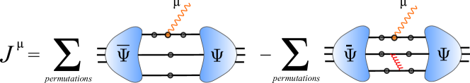
Figure 2: Diagrams necessary to calculate the current $J^{\mu}$, describing the coupling of an external photon field to a baryon, described by the Faddeev amplitude $\Psi$, in the RL truncation.

The current $J^{\mu}$ describing the coupling of a baryon to an external electromagnetic current in the RL truncation is given by the sum

$$J_{\mathcal{I}^{\prime}\mathcal{I}}^{\mu}=\sum_{\rho\rho^{\prime};\lambda}( \mathcal{Q}^{\rho\rho^{\prime};\lambda}_{1}(J_{1}^{\rho\rho^{\prime};\lambda})_{\mathcal{I}^{\prime}\mathcal{I}}^{\mu}+\mathcal{Q}^{\rho\rho^{\prime};\lambda}_{2}(J_{2}^{\rho\rho^{\prime};\lambda})_{\mathcal{I}^{\prime}\mathcal{I}}^{\mu}+$$

$$\mathcal{Q}^{\rho\rho^{\prime};\lambda}_{3}(J_{3}^{\rho\rho^{\prime};\lambda})_{\mathcal{I}^{\prime}\mathcal{I}}^{\mu})~{},$$ (8)

with

$$(J_{1}^{\rho\rho^{\prime};\lambda})_{\mathcal{I}^{\prime}\mathcal{I}}^{\mu} =\int_{p}\int_{q}\bar{\Psi}^{\rho}_{\beta^{\prime}\alpha^{\prime}\mathcal{I}^{\prime}\gamma^{\prime}}(p_{f}^{\{1\}},q^{\{1\}}_{f},P_{f})\times$$

$$\left[\left(S^{(\lambda_{1})}(p_{1}^{f})\Gamma^{\mu}(p_{1},Q)S^{(\lambda_{1})}(p_{1}^{i})\right)_{\alpha^{\prime}\alpha}\right.\times$$

$$\vspace*{0mm}\left.S^{(\lambda_{2})}_{\beta^{\prime}\beta}(p_{2})S^{(\lambda_{3})}_{\gamma^{\prime}\gamma}(p_{3})\right]\times$$

$$\vspace*{0mm}\left(\Psi^{\rho^{\prime}}_{\alpha\beta\gamma\mathcal{I}}(p^{\{1\}}_{i},q^{\{1\}}_{i},P_{i})-\Psi^{\{1\};\lambda}_{\alpha\beta\gamma\mathcal{I}}(p^{\{1\}}_{i},q^{\{1\}}_{i},P_{i})\right),$$

$$(J_{2}^{\rho\rho^{\prime};\lambda})_{\mathcal{I}^{\prime}\mathcal{I}}^{\mu} =\int_{p}\int_{q}\bar{\Psi}^{\rho}_{\beta^{\prime}\alpha^{\prime}\mathcal{I}^{\prime}\gamma^{\prime}}(p^{\{2\}}_{f},q^{\{2\}}_{f},P_{f})\left[S^{(\lambda_{1})}_{\alpha^{\prime}\alpha}(p_{1})\right.\times$$

$$\left.\left(S^{(\lambda_{2})}(p_{2}^{f})\Gamma^{\mu}(p_{2},Q)S^{(\lambda_{2})}(p_{2}^{i})\right)_{\beta^{\prime}\beta}S^{(\lambda_{3})}_{\gamma^{\prime}\gamma}(p_{3})\right]\times$$

$$\left(\Psi^{\rho^{\prime}}_{\alpha\beta\gamma\mathcal{I}}(p^{\{2\}}_{i},q^{\{2\}}_{i},P_{i})-\Psi^{\{2\};\lambda}_{\alpha\beta\gamma\mathcal{I}}(p^{\{2\}}_{i},q^{\{2\}}_{i},P_{i})\right),$$

$$(J_{3}^{\rho\rho^{\prime};\lambda})_{\mathcal{I}^{\prime}\mathcal{I}}^{\mu} =\int_{p}\int_{q}\bar{\Psi}^{\rho}_{\beta^{\prime}\alpha^{\prime}\mathcal{I}^{\prime}\gamma^{\prime}}(p^{\{3\}}_{f},q^{\{3\}}_{f},P_{f})\times$$

$$\left[S^{(\lambda_{1})}_{\alpha^{\prime}\alpha}(p_{1})S^{(\lambda_{2})}_{\beta^{\prime}\beta}(p_{2})\right.\times$$

$$\left.\left(S^{(\lambda_{3})}(p_{3}^{f})\Gamma^{\mu}(p_{3},Q)S^{(\lambda_{3})}(p_{3}^{i})\right)_{\gamma^{\prime}\gamma}\right]\times$$

$$\left(\Psi^{\rho^{\prime}}_{\alpha\beta\gamma\mathcal{I}}(p^{\{3\}}_{i},q^{\{3\}}_{i},P_{i})-\Psi^{\{3\};\lambda}_{\alpha\beta\gamma\mathcal{I}}(p^{\{3\}}_{i},q^{\{3\}}_{i},P_{i})\right),$$ (9)

where we have defined

$$\Psi^{\{1\};\lambda}_{\alpha\beta\gamma\mathcal{I}}=\int_{k}\widetilde{K}_{\beta\beta^{\prime}\gamma\gamma^{\prime}}(k) S^{(\lambda_{2})}_{\beta^{\prime}\beta^{\prime\prime}}(p_{2}-k)S^{(\lambda_{3})}_{\gamma^{\prime}\gamma^{\prime\prime}}(p_{3}+k)$$

$$\Psi_{\alpha\beta^{\prime\prime}\gamma^{\prime\prime}\mathcal{I}}(p+k,q-k/2,P)~{},$$ (10)

as a result of the first term in the Faddeev equation and similarly we define $\Psi^{\{2\};\lambda}$ and $\Psi^{\{3\};\lambda}$. The transferred photon momentum $Q$ is introduced via the final and initial momenta of the interacting quark $\kappa$

$$p_{\kappa}^{\nicefrac{{f}}{{i}}}=p_{\kappa}\pm\frac{Q}{2}~{}.$$ (11)

which also implies $Q=P_{f}-P_{i}$. The relative momenta in the respective terms of (2.1) are defined in Appendix D. The charge matrices are defined as

$$\mathcal{Q}^{\rho\rho^{\prime};\lambda}_{1} =F^{\rho}_{abc}\textrm{Q}_{aa^{\prime}}F^{\rho^{\prime},\lambda}_{a^{\prime}bc}$$

$$\mathcal{Q}^{\rho\rho^{\prime};\lambda}_{2} =F^{\rho}_{abc}\textrm{Q}_{bb^{\prime}}F^{\rho^{\prime},\lambda}_{ab^{\prime}c}$$ (12)

$$\mathcal{Q}^{\rho\rho^{\prime};\lambda}_{3} =F^{\rho}_{abc}\textrm{Q}_{cc^{\prime}}F^{\rho^{\prime},\lambda}_{abc^{\prime}}$$

with Q the charge operator

$$\textrm{Q}=\left(\begin{array}[]{ccc}\nicefrac{{2}}{{3}}&0&0\\ 0&-\nicefrac{{1}}{{3}}&0\\ 0&0&-\nicefrac{{1}}{{3}}\end{array}\right)~{}.$$ (16)

The three terms in (2.1) can be related to each other in the same fashion as Eq. (2), so that only one term needs to be solved explicitly. It can be shown Eichmann:2011vu that

$$J_{\mathcal{I}^{\prime}\mathcal{I}}^{\mu}=\sum_{\rho\rho^{\prime};\lambda}( \mathcal{Q}^{\rho\rho^{\prime}}_{1}(\mathcal{F}_{1}^{\rho\rho^{\prime}}J_{3}^{\rho^{\prime}\rho^{\prime\prime};\lambda}\mathcal{F}_{1}^{T,\rho^{\prime\prime}\rho})_{\mathcal{I}^{\prime}\mathcal{I}}^{\mu}+$$

$$\mathcal{Q}^{\rho\rho^{\prime}}_{2}(\mathcal{F}_{2}^{\rho\rho^{\prime}}J_{3}^{\rho^{\prime}\rho^{\prime\prime};\lambda}\mathcal{F}_{2}^{T,\rho^{\prime\prime}\rho})_{\mathcal{I}^{\prime}\mathcal{I}}^{\mu}+$$

$$\mathcal{Q}^{\rho\rho^{\prime}}_{3}(J_{3}^{\rho\rho^{\prime};\lambda})_{\mathcal{I}^{\prime}\mathcal{I}}^{\mu})~{},$$ (17)

with the matrices $\mathcal{F}$ and the results of the flavour contractions above for the different baryons given in Appendix C.

Finally, the quark-photon vertex $\Gamma^{\mu}$ is calculated from an inhomogenous Bethe-Salpeter equation

$$\Gamma^{\mu}(p,Q) =iZ_{2}\gamma^{\mu}$$

$$+\int_{k}K_{q\bar{q}}\left(S(k+Q/2)\Gamma^{\mu}(k,Q)S(k-Q/2)\right)~{},$$ (18)

and using for $K_{q\bar{q}}$ the RL kernel (20) with $C=4/3$ and for the quark propagator $S$ the solutions of the RL-truncated quark DSE.

2.2 Effective coupling of one-gluon exchange

For the effective interaction in the RL truncation we use the Maris-Tandy model Maris:1997tm ; Maris:1999nt which has been employed frequently in hadron studies within the rainbow-ladder BSE/DSE framework. The advantages of this model are its simplicity and that it performs very well for phenomenological calculations of ground-state meson and baryon properties in most channels. It can be defined via the combination of the relevant parts in the quark self-energy

$$Z_{1f}C_{F}\frac{g^{2}}{4\pi}D_{\mu\nu}(k)\Gamma^{\nu}(p,q)=Z_{2}^{2}C_{F}T_{\mu\nu}^{k}\frac{\alpha_{\mathrm{eff}}(k^{2})}{k^{2}}\gamma^{\nu}\;,$$ (19)

with $\alpha_{\mathrm{eff}}(k^{2})$ the effective coupling. In this way the resulting kernel in the BSE is given by

$${K}^{RL}_{\alpha\alpha^{\prime}\beta^{\prime}\beta}(k)=-4\pi C_{F}~{}Z_{2}^{2}~{}\frac{\alpha_{\textrm{eff}}(k^{2})}{k^{2}}~{}T_{\mu\nu}(k)~{}\gamma^{\mu}_{\alpha\alpha^{\prime}}\gamma^{\nu}_{\beta^{\prime}\beta}\,\,.$$ (20)

with gluon momentum $k=p-q$ and transverse projector $T_{\mu\nu}(k)=\delta^{\mu\nu}-\hat{k}^{\mu}\hat{k}^{\nu}$. The effective running coupling $\alpha_{\textrm{eff}}$ is finally given by

$$\alpha_{\textrm{eff}}(k^{2}){}= \pi\eta^{7}\left(\frac{k^{2}}{\Lambda^{2}}\right)^{2}e^{-\eta^{2}\frac{k^{2}}{\Lambda^{2}}}$$

$$+{}\frac{2\pi\gamma_{m}\big{(}1-e^{-k^{2}/\Lambda_{t}^{2}}\big{)}}{\textnormal{ln}[e^{2}-1+(1+k^{2}/\Lambda_{QCD}^{2})^{2}]}\,.$$ (21)

This interaction reproduces the one-loop QCD behaviour of the quark propagator at large momenta and the Gaussian distribution of interaction strength in the intermediate momentum region provides enough strength for dynamical chiral symmetry breaking to take place. The scale $\Lambda_{t}=1$ GeV is introduced for technical reasons and has no impact on the results. For the anomalous dimension we use $\gamma_{m}=12/(11N_{C}-2N_{f})=12/25$, corresponding to $N_{f}=4$ flavours and $N_{c}=3$ colours. The scale in the ultraviolet part of the coupling is set to $\Lambda_{QCD}=0.234$ GeV.

Table 1: Hyperon masses (in GeV) from the rainbow-ladder truncated Faddeev equation. We give the central value of the bands corresponding to a variation of $\eta$ between $1.6$ and $2.0$ with the halfwidth of the bands added in brackets. We compare also with experimental values Beringer:1900zz .

	$\Sigma/\Lambda$	$\Xi$	$\Sigma^{*}$	$\Xi^{*}$
Faddeev	1.073 (1)	1.235 (5)	1.33 (2)	1.47(3)
Experiment	1.189/1.116	1.315	1.385 (2)	1.533 (2)
Relative difference	10/4 %	6 %	4 %	4 %

In the infrared momentum region, the interaction strength is characterised by a scale $\Lambda$ and a dimensionless parameter $\eta$ that controls the width of the interaction. The scale $\Lambda=0.72$ GeV is adjusted to reproduce the experimental pion decay constant from the truncated pion BSE. This as well as many other pseudo-scalar ground-state observables, such as the masses of ground-state mesons and baryons, turn out to be almost insensitive to the value of $\eta$ in the range of values of $\eta$ between $1.6$ and $2.0$ see, e.g. Krassnigg:2009zh ; Nicmorus:2010mc ; Eichmann:2011vu ). The $u/d$ and $s$ current-quark masses are fixed to reproduce the physical pion and kaon masses, respectively. The corresponding values are $m_{u/d}(\mu^{2})=3.7$ MeV and $m_{s}(\mu^{2})=85$ MeV. The renormalisation scale is chosen to be $\mu^{2}=(19\,\mbox{GeV})^{2}$.

3 Results

We have calculated the electromagnetic elastic form factors for all lowest-lying hyperons of the spin-$\nicefrac{{1}}{{2}}$ isospin octet and spin-$\nicefrac{{3}}{{2}}$ isospin decuplet. In the plots below we present (coloured bands) the numerical results for values of the $\eta$ parameter between $\eta=1.6$ and $\eta=2.0$. Moreover, we show fits of our results using a generalised multipole expression

$$G(Q^{2})=\frac{n_{0}+n_{1}Q^{2}}{1+d_{1}Q^{2}+d_{2}Q^{4}+d_{3}Q^{6}+d_{4}Q^{8}}\,.$$ (22)

For analogous calculations of form factors of non-strange baryons and the Omega resonance we refer the reader to Eichmann:2011vu ; Sanchis-Alepuz:2013iia .

Before we discuss the results it is worth summarising the main strengths and weaknesses of the rainbow-ladder truncation scheme used in the present calculation, in order to facilitate the subsequent interpretation of results:

• Ground-state baryon masses obtained from the present formalism in the RL truncation, in combination with the Maris-Tandy model from Eq. (2.2), show excellent agreement with experimental data. In the case of baryons with strange quarks the small differences can be attributed to the lack of quark-mass dependence of the interaction (see table 1).

• Results for nucleon, Delta and Omega electromagnetic form factors Eichmann:2011vu ; Sanchis-Alepuz:2013iia are consistent with a quark-core picture. That is, since meson-cloud effects are not taken into account, form factors for low-$Q^{2}$ are consistently underestimated. In the high-$Q^{2}$ region, where the effect of the meson cloud is small, the agreement with experimental and/or lattice data is however excellent.

• With our current computational techniques, calculations are limited to a maximum value of $Q^{2}$ due to the presence of complex conjugate poles in the quark propagators (see Appendix D and e.g. Eichmann:2011aa ; Dorkin:2013rsa ). The specific values of these limits depend on the masses of the baryons of interest. Nevertheless in most cases results are still smooth beyond these regions. This can be seen e.g. in the electric form factor of the $\Sigma_{0}$, Fig. 3, for $Q^{2}\geq 2.25$ GeV². With due caution, extrapolations for high-$Q^{2}$ values are thus possible.

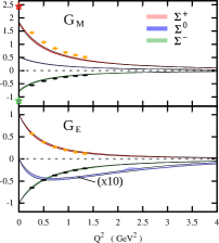
Figure 3: Magnetic (upper panel) and electric (lower panel) form factors for the octet Sigma triplet. The magnetic form factor is given in units of the nuclear magneton $\mu_{N}$. Coloured bands represent the result of the numerical calculation for $\eta=[1.6,2.0]$. Stars indicate experimental values. For finite $Q^{2}$ we also include lattice data from Shanahan:2014uka ; Shanahan:2014cga . Solid black lines are our best fits for $\eta=1.6$ and $\eta=2.0$.

3.1 Octet hyperons

The elastic coupling of a spin$-\nicefrac{{1}}{{2}}$ baryon to an external electromagnetic field is described by the following current

$$J^{\mu}\left(Q,P\right)=i\Lambda_{+}(P_{f}) \left(F_{1}(Q^{2})\gamma^{\mu}\right.$$

$$\left.-\frac{F_{2}(Q^{2})}{2M}\sigma^{\mu\nu}Q^{\nu}\right)\Lambda_{+}(P_{i})\,,$$ (23)

parametrized by the two Dirac form factors $F_{1}$ and $F_{2}$ and with $\Lambda^{+}(\hat{P})=\left(\mathds{1}+\ooalign{\hfil/\hfil\crcr$\hat{P}$}\right)/2$ the positive-energy projector. We present here results for the electric and magnetic Sachs form factors

$$G_{E}(Q^{2}) =F_{1}(Q^{2})-\frac{Q^{2}}{2M^{2}}F_{2}(Q^{2})~{},$$ (24)

$$G_{M}(Q^{2}) =F_{1}(Q^{2})+F_{2}(Q^{2})~{}.$$ (25)

In the case of the baryon octet, experimental data exist for the magnetic moment of all members of the octet and for the electric radius of the nucleon and the $\Sigma^{-}$. In addition, precise lattice QCD data for non-vanishing momentum transfer up to $Q^{2}=1.3~{}$GeV² are now available Shanahan:2014uka ; Shanahan:2014cga .

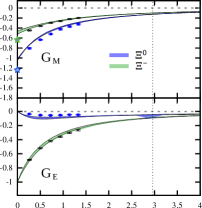
Figure 4: Magnetic (upper panel) and electric (lower panel) form factors for the octet Xi doublet. The magnetic form factor is given in units of the nuclear magneton $\mu_{N}$. Coloured bands represent the result of the numerical calculation for $\eta=[1.6,2.0]$. Stars indicate experimental values. For finite $Q^{2}$ we also include lattice data from Shanahan:2014uka ; Shanahan:2014cga . Solid black lines are our best fits for $\eta=1.6$ and $\eta=2.0$. Vertical dotted lines indicate the region beyond which the singularities of the quark propagator are probed.

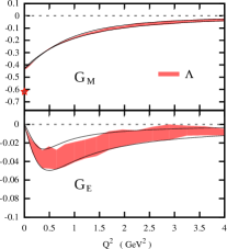
Figure 5: Magnetic (upper panel) and electric (lower panel) form factors for the Lambda singlet. The magnetic form factor is given in units of the nuclear magneton $\mu_{N}$. Coloured bands represent the result of the numerical calculation for $\eta=[1.6,2.0]$. Solid black lines are our best fits for $\eta=1.6$ and $\eta=2.0$.

In figures 3, 4 and 5 we show the electric and magnetic form factors of the Sigma and Xi multiplets and the Lambda singlet. We compare our results with experimental data for the magnetic moments Agashe:2014kda and with lattice QCD data determined from $N_{f}=2+1$ dynamical configurations under the omission of disconnected diagrams. The lattice results have been obtained at unphysical pion masses and extrapolated to the physical point using partially quenched chiral perturbation theory Shanahan:2014uka ; Shanahan:2014cga . The systematic error associated with this setup is arguably smaller than the one induced by the omission of meson cloud effects in our results.

For the charged $\Sigma$ baryons and for the $\Xi$ doublet our results show an overall good agreement with the corresponding lattice data. This is particularly true for the electric form factors, which are protected in the infrared by charge conservation. In the magnetic sector we observe an interesting pattern. While $G_{M}$ for the $\Sigma^{-}$ and $\Xi^{-}$ agree well with the lattice data at finite $Q^{2}$, there is a significant deviation for the $\Sigma^{+}$ and the $\Xi^{0}$. At $Q^{2}=0$ the deviation of our magnetic moment with the experimental value is similar in relative size for the $\Sigma^{+}$ and the $\Sigma^{-}$, whereas it is much smaller for the $\Xi^{+}$ than for the $\Xi^{0}$, see Tab. 2.

This pattern may be understood from the different influence and the interplay of pion and kaon cloud effects on the various states Leinweber:2002qb ; Boinepalli:2006xd . For the $\Sigma^{\pm}$-states, pion cloud effects play an important role for both states at small $Q^{2}$, leading to the observed discrepancies of our magnetic moments with the experimental values. For larger values of $Q^{2}$ also kaon cloud effects are important, which are strong only in the $\Sigma^{+}$-channel. This may explain the better agreement of our results with the lattice data for $\Sigma^{-}$. For the $\Xi$-states, pion cloud effects are small and kaon cloud effects are much larger in the $\Xi^{0}$ than in the $\Xi^{-}$. As a consequence we observe only small deviations of the magnetic moment of the $\Xi^{-}$ with experiment and also much better agreement with the lattice data than for the $\Xi^{0}$.

Table 2: Magnetic moments $\mu$ (in units of the nuclear magneton $\mu_{N}$) of the octet hyperons, compared to experimental values Agashe:2014kda . Electric and magnetic mean-square radii (in fm²) of the octet hyperons.

	$\mu$	$\mu_{exp}$	$\langle r^{2}_{E}\rangle$	$\langle r^{2}_{M}\rangle$
$\Sigma^{+}$	1.82(2)	2.46(1)	0.56(3)	0.43(2)
$\Sigma^{0}$	0.521(1)	–	0.057(8)	0.39(3)
$\Sigma^{-}$	-0.78(2)	-1.16(3)	0.45(3)	0.50(1)
$\Xi^{0}$	-1.05(1)	-1.250(14)	0.10(1)	0.35(3)
$\Xi^{-}$	-0.57(4)	-0.651(3)	0.37(4)	0.20(2)
$\Lambda$	-0.435(5)	-0.613(4)	0.04(1)	0.21(1)

Clearly, in the future we need to include the effects of the pion and kaon cloud in our calculations. First steps in this direction have been performed on the level of meson and baryon masses in Refs. Fischer:2008sp ; Fischer:2008wy ; Sanchis-Alepuz:2014wea . The generalisation of this framework to include form factors is under way.

For high-$Q^{2}$ values the effect of the meson cloud diminishes and we can see that in Figs. 3 and 4 the agreement with lattice data improves. This fact encourages us to consider our results as a good representation of hyperon form factors for $Q^{2}$ values which are inaccessible to lattice QCD with the present computing capabilities. It, moreover, supports the predictive value of our results, for moderate to high-$Q^{2}$, in those cases in which lattice data is not available, such as for $\Sigma^{0}$ and $\Lambda$ baryons or for decuplet hyperons (see below).

It is straightforward in our framework to extract the corresponding electric or magnetic distribution radius using the formula

$$\langle r^{2}\rangle_{G}=-\frac{6}{G(0)}\left.\frac{dG(Q^{2})}{dQ^{2}}\right|_{Q^{2}=0}~{},$$ (26)

where the term $G(0)$ is set to one for form factors constrained to vanish at the origin. The results for the electric and magnetic square radii are shown in Tab. 2. For these observables, only the electric radius of $\Sigma^{-}$ is known experimentally, $r^{2}_{E,\Sigma^{-}}=0.60~{}$fm². As expected with the absence of a long range meson cloud, our results underestimate the experimental value. Even though a quantitative prediction of charge and magnetic radii will have to wait until meson cloud effects can be taken into account in our approach, there are a number of qualitative features worth discussing, since these will presumably survive in a more complete calculation: Despite having equal quark content, the electric radius of $\Sigma^{0}$ is larger than that of the $\Lambda$. In constituent quark models this is usually interpreted in a two-step way: in the $\Lambda$ a scalar, isoscalar diquark is formed between the non-strange quarks whereas in the $\Sigma^{0}$ the scalar diquark is formed between strange and non-strange quarks. In the latter case, repulsive hyperfine interaction in the non-strange sector makes the charge distribution broader. As already discussed in Boinepalli:2006xd , confirmed in Boinepalli:2009sq and also in our calculation (see Tab. 3 below), this explanation is in contradiction with the fact that decuplet hyperons are slightly smaller than their octet counterparts. In the decuplet, there is no reason why scalar diquarks should dominate and thus charge distributions should be broader, which is not the case. Thus one needs to resort to alternative explanations. In Boinepalli:2006xd the difference between the electric radii of $\Sigma^{0}$ and $\Lambda$ is associated to the different intermediate virtual transitions influencing each baryon. We do not include such intermediate states in our present calculation, but still see this difference. Thus from our framework we conclude that the difference may be merely due to the different flavour symmetry of both states.

It is also interesting to note how for the magnetic radii some patterns are reversed. Whereas the electric distribution is broader in the $\Sigma^{+}$ than in the $\Sigma^{-}$ and also in the $\Xi^{0}$ than in $\Xi^{-}$, the opposite occurs for the magnetic distribution. This pattern is also observed in lattice calculations Boinepalli:2006xd ; Shanahan:2014uka . Moreover, $\Sigma^{-}$ has the largest magnetic radius of all octet members, a feature also seen in Boinepalli:2006xd ; Shanahan:2014uka .

Finally we wish to mention that in contrast to all other form factors, it was impossible to fit the $\Sigma^{0}$ form factors with a dipole-like expression. In order to obtain a good representation we had to include terms up to ${\sim}Q^{8}$ in the denominator of Eq. (33), see Tab. 4 in the appendix.

3.2 Decuplet hyperons

The elastic coupling of a spin$-\nicefrac{{3}}{{2}}$ baryon to an external electromagnetic field is described by the following current

$$J^{\mu,\alpha\beta}(P,Q)={} \mathbb{P}^{\alpha\alpha^{\prime}}(\hat{P}_{f})\left[\left((F_{1}+F_{2})i\gamma^{\mu}-F_{2}\frac{P^{\mu}}{M}\right)\delta^{\alpha^{\prime}\beta^{\prime}}\right.$$

$$+\left.\left((F_{3}+F_{4})i\gamma^{\mu}-F_{4}\frac{P^{\mu}}{M}\right)\frac{Q^{\alpha^{\prime}}Q^{\beta^{\prime}}}{4M^{2}}\right]$$

$$~{}\hskip 110.96574pt\mathbb{P}^{\beta^{\prime}\beta}(\hat{P}_{i})$$ (27)

where $\mathbb{P}$ is the Rarita-Schwinger projector

$$\mathbb{P}_{+}^{\mu\nu}(\hat{P})= ~{}\Lambda_{+}(\hat{P})\left(T_{P}^{\mu\nu}-\frac{1}{3}\gamma^{\mu}_{T}\gamma^{\nu}_{T}\right)~{}.$$ (28)

The current is now parameterised by the four form factors $F_{i}$, $i\in\{1,...,4\}$. We present results in terms of the Sachs form factors known as the electric monopole ($G_{E_{0}}(Q^{2})$), magnetic dipole ($G_{M_{1}}(Q^{2})$), electric quadrupole ($G_{E_{2}}(Q^{2})$) and magnetic octupole ($G_{M_{3}}(Q^{2})$) form factors, defined by

$$G_{E_{0}} =\left(1+\frac{2\tau}{3}\right)(F_{1}-\tau F_{2})-\frac{\tau}{3}(1+\tau)\,(F_{3}-\tau F_{4})\,,$$ (29)

$$G_{M_{1}} =\left(1+\frac{4\tau}{5}\right)(F_{1}+F_{2})-\frac{2\tau}{5}(1+\tau)\,(F_{3}+F_{4})\,,$$ (30)

$$G_{E_{2}} =(F_{1}-\tau F_{2})-\frac{1}{2}\,(1+\tau)\,(F_{3}-\tau F_{4})\,,$$ (31)

$$G_{M_{3}} =(F_{1}+F_{2})-\frac{1}{2}\,(1+\tau)\,(F_{3}+F_{4})\,,$$ (32)

with $\tau=Q^{2}/4M^{2}$.

Whereas for the Delta baryon lattice QCD data of the $Q^{2}$ evolution of form factors exists, for the strange members of the decuplet only static properties have been calculated on the lattice Boinepalli:2009sq . Considering the good comparison with lattice data in the case of octet baryons in this paper and in Ref. Eichmann:2011vu as well as for the Delta in Ref. Sanchis-Alepuz:2013iia , we can regard the results presented below as qualitative predictions for moderate $Q^{2}$ which become quantitative predictions at higher $Q^{2}$.

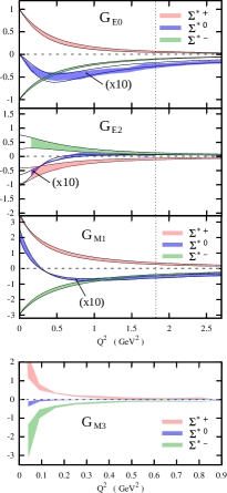
Figure 6: Electric monopole, electric quadrupole, magnetic dipole and magnetic octupole form factors for the Sigma triplet. Coloured bands represent the result of the numerical calculation for $\eta=[1.6,2.0]$. Solid black lines are our best fits for $\eta=1.6$ and $\eta=2.0$. Vertical dotted lines indicate the region beyond which the singularities of the quark propagator are probed.

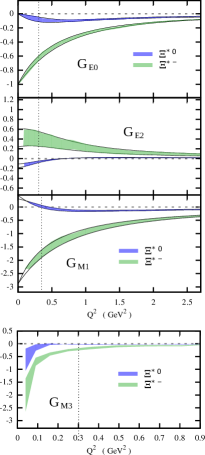
Figure 7: Electric monopole, electric quadrupole, magnetic dipole and magnetic octupole form factors for the Xi doublet. Coloured bands represent the result of the numerical calculation for $\eta=[1.6,2.0]$. Solid black lines are our best fits for $\eta=1.6$ and $\eta=2.0$. Vertical dotted lines indicate the region beyond which the singularities of the quark propagator are probed.

In Fig. 6 we show our results for the electric monopole $G_{E_{0}}$ and quadrupole $G_{E_{2}}$ form factors. It is interesting to note that the form factors corresponding to $\Sigma^{*~{}0}$ are not vanishing. Moreover, the electric monopole form factor is of the same order as the analogous $G_{E}$ of its octet counterpart. This is in contrast with the Delta baryon multiplet. In that case, $SU(2)$ isospin symmetry implies (in the case of a flavour diagonal interaction like the RL kernel) that the form factors are proportional to the baryon charge, thus implying that all form factors of the $\Delta^{0}$ vanish identically.

The electric quadrupole form factor provides a measure of the deviation of the charge distribution from sphericity Nozawa:1990gt ; Buchmann:2002xq ; Pascalutsa:2006up . We predict a prolate (positive $G_{E_{2}}$) shape for the charge distribution in $\Sigma^{*~{}+}$ and oblate (negative sign) for the $\Sigma^{*~{}-}$. In the case of the $\Sigma^{*~{}0}$ we even obtain a zero crossing at $Q^{2}\sim 700$MeV, the charge distribution changing from an oblate to a prolate shape as the electromagnetic probe increases in energy. It will be interesting to check whether this feature survives a more sophisticated calculation in an extension of the present framework including meson cloud effects. Furthermore, a remark on the calculation of $G_{E_{2}}$ for small values of $Q^{2}$ is in order: it can be seen from Eq. (37), that the equation to extract $G_{E_{2}}$ from traces of the current (3.2) features a $Q^{-4}$ factor which should be compensated by cancellations of other terms in order to give a finite value of $G_{E_{2}}$ at $Q^{2}\sim 0$. With the accuracy of our current calculations this cancellation is not exact and numerical noise appears. This is manifested in the plots by the coloured bands stopping at a small but non-zero value of $Q^{2}$ (see also Sanchis-Alepuz:2013iia ).

A similar discussion applies for the electric monopole and quadrupole form factors of the $\Xi^{*~{}0}$ $\Xi^{*~{}-}$ hyperons from Fig. 7. The form factors of $\Xi^{*~{}0}$ are not vanishing and $G_{E_{0}}$ is of the same order as $G_{E}$ for $\Xi^{0}$. The quadrupole form factor $G_{E_{2}}$ also features a zero crossing for the $\Xi^{*~{}0}$, but this time in the region in which the singularities of the quark propagator are probed (see discussion above and Appendix D) and our predictions are less reliable.

From the electric monopole form factors we can extract the electric radii. Our results are given in Tab. 3. As already mentioned in the previous section, all strange members of the decuplet have a similar or slightly smaller size that their octet counterparts. It will be interesting to study whether the different effect of the meson cloud in octet and decuplet states alters this feature.

Table 3: Electric-$E_{0}$ and magnetic-$M_{1}$ mean-square radii of the decuplet hyperons in units of (fm)².

	$\Sigma^{*+}$	$\Sigma^{*0}$	$\Sigma^{*-}$	$\Xi^{*0}$	$\Xi^{*-}$
$\langle r^{2}_{E0}\rangle$	0.55(4)	0.04(1)	0.51(5)	0.08(6)	0.38(7)
$\langle r^{2}_{M1}\rangle$	0.42(5)	1.36(4)	0.31(4)	0.38(7)	0.41(10)

The magnetic dipole $G_{M_{1}}$ and octupole $G_{M_{3}}$ form factors are shown in the two lower panels of Figs. 6 and 7 for the $\Sigma^{*}$ triplet and the $\Xi^{*}$ doublet respectively. The most interesting feature is again a zero crossing of the dipole form factor for the neutral members $\Sigma^{*~{}0}$ and $\Xi^{*~{}0}$.

From the magnetic dipole $G_{M_{1}}$ form factor we extract the magnetic radii, shown in Tab. 3. The most remarkable and puzzling feature of this calculation is the enormous magnetic radius of the neutral $\Sigma^{*~{}0}$. The reason for this deviation in comparison with the other decuplet states is not clear to us. Note that also in a quark model calculation of these observables Wagner:2000ii , the $\Sigma^{*~{}0}$ (together with the $\Xi^{*~{}0}$) has the largest magnetic radius of all ground-state hyperons. The differences are, however, much smaller than in our calculation.

Finally, with respect to the magnetic octupole form factors, the factor $Q^{-6}$ in the extraction of the form factor (39) prevents us, with our current accuracy, to extract precise results. The only feature that seems robust at the present stage is the sign of the corresponding form factor. As with $G_{E_{2}}$, a non-vanishing $G_{M_{3}}$ indicates a deformation of the magnetic distribution, with a positive (negative) sign signalling a prolate (oblate) shape.

4 Summary

We have presented results for the elastic electromagnetic form factors of all ground-state hyperons in the rainbow ladder truncation of the covariant three-body Bethe-Salpeter equation. Our results have been compared with lattice QCD data where available, showing good agreement with small deviations in some isospin channels that can be explained. At vanishing momentum transfer, where experimental data exists for the members of the isospin octet, is where the largest deviations appear. We interpret this as a manifestation of the absence of a pion and kaon cloud in the present calculation. Similar discrepancies have been observed previously in the calculation of non-strange baryon form factors Eichmann:2011vu ; Eichmann:2011pv ; Sanchis-Alepuz:2013iia . Including such effects is a necessary next step and work in this direction based on Fischer:2008sp ; Fischer:2008wy ; Sanchis-Alepuz:2014wea is in progress.

5 Acknowledgements

This work has been supported by an Erwin Schrödinger fellowship J3392-N20 from the Austrian Science Fund, FWF, by the Helmholtz International Center for FAIR within the LOEWE program of the State of Hesse, and by the DFG collaborative research centre TR 16.

Appendix A Fits for form factors

In order to facilitate the use of our results for other calculations, we have fitted them using the following general rational form

$$G(Q^{2})=\frac{n_{0}+n_{1}Q^{2}}{1+d_{1}Q^{2}+d_{2}Q^{4}+d_{3}Q^{6}+d_{4}Q^{8}}~{}.$$ (33)

Our aim has been to use the polynomials of lowest order possible in the denominator that reproduce the calculated form factors. The resulting fitting parameters are shown in tables 4 and 5.

	$G_{E}~{}(\eta=1.6)$	$G_{E}~{}(\eta=2.0)$	$G_{M}~{}(\eta=1.6)$	$G_{M}~{}(\eta=2.0)$
$\Sigma^{+}$	$n_{0}=1$	$n_{0}=1$	$n_{0}=2.139$	$n_{0}=2.082$
	$d_{1}=2.249$	$d_{1}=2.503$	$d_{1}=1.767$	$d_{1}=1.944$
	$d_{2}=1.528$	$d_{2}=1.981$	$d_{2}=0.654$	$d_{2}=0.607$
$\Sigma^{0}$	$n_{1}=-0.209$	$n_{1}=-0.284$	$n_{0}=0.606$	$n_{0}=0.603$
	$d_{1}=1.766$	$d_{1}=2.914$	$d_{1}=1.575$	$d_{1}=1.792$
	$d_{2}=2.666$	$d_{2}=2.351$	$d_{2}=0.608$	$d_{2}=0.555$
	$d_{3}=-0.872$	$d_{3}=-0.327$
	$d_{4}=0.425$	$d_{4}=0.282$
$\Sigma^{-}$	$n_{0}=-1$	$n_{0}=-1$	$n_{0}=-0.928$	$n_{0}=-0.877$
	$d_{1}=1.801$	$d_{1}=2.020$	$d_{1}=2.044$	$d_{1}=2.166$
	$d_{2}=0.651$	$d_{2}=0.641$	$d_{2}=0.743$	$d_{2}=0.710$
$\Xi^{0}$	$n_{1}=-0.473$	$n_{1}=-0.434$	$n_{0}=-1.383$	$n_{0}=-1.399$
	$d_{1}=2.886$	$d_{1}=0.513$	$d_{1}=1.363$	$d_{1}=1.582$
	$d_{2}=2.253$	$d_{2}=3.135$	$d_{2}=0.355$	$d_{2}=0.346$
$\Xi^{-}$	$n_{0}=-1$	$n_{0}=-1$	$n_{0}=-0.705$	$n_{0}=-0.613$
	$d_{1}=1.450$	$d_{1}=1.774$	$d_{1}=0.928$	$d_{1}=0.783$
	$d_{2}=0.634$	$d_{2}=0.588$	$d_{2}=0.168$	$d_{2}=0.172$
$\Lambda$	$n_{1}=-0.092$	$n_{1}=-0.203$	$n_{0}=-0.505$	$n_{0}=-0.498$
	$d_{1}=-1.732$	$d_{1}=0.049$	$d_{1}=0.826$	$d_{1}=0.971$
	$d_{2}=6.262$	$d_{2}=4.056$	$d_{2}=0.757$	$d_{2}=0.339$

Table 4: Fitting parameters for the elastic form factors of the strange members of the baryon octet.

	$G_{E0}~{}(\eta=1.6)$	$G_{E0}~{}(\eta=2.0)$	$G_{E2}~{}(\eta=1.6)$	$G_{E2}~{}(\eta=2.0)$	$G_{M1}~{}(\eta=1.6)$	$G_{M1}~{}(\eta=2.0)$
$\Sigma^{*+}$	$n_{0}=1$	$n_{0}=1$	$n_{0}=-1.040$	$n_{0}=-0.393$	$n_{0}=3.392$	$n_{0}=3.606$
	$d_{1}=2.197$	$d_{1}=2.514$	$n_{1}=-0.555$	$n_{1}=-0.248$	$d_{1}=2.766$	$d_{1}=3.590$
	$d_{2}=2.897$	$d_{2}=5.875$	$d_{1}=1.932$	$d_{1}=0.123$	$d_{2}=0.940$	$d_{2}=2.011$
			$d_{2}=3.765$	$d_{2}=3.812$
$\Sigma^{*0}$	$n_{1}=-0.116$	$n_{1}=-0.208$	$n_{0}=-0.097$	$n_{0}=-0.066$	$n_{0}=0.190$	$n_{0}=0.250$
	$d_{1}=-1.341$	$d_{1}=-0.872$	$n_{1}=0.172$	$n_{1}=0.079$	$n_{1}=-0.701$	$n_{1}=-0.851$
	$d_{2}=3.985$	$d_{2}=4.498$	$d_{1}=-1.637$	$d_{1}=-0.159$	$d_{1}=4.020$	$d_{1}=2.316$
			$d_{2}=10.525$	$d_{2}=4.418$	$d_{2}=0.031$	$d_{2}=3.665$
					$d_{3}=3.550$	$d_{3}=0.600$
					$d_{4}=-0.567$	$d_{4}=-0.020$
$\Sigma^{*-}$	$n_{0}=-1$	$n_{0}=-1$	$n_{0}=0.762$	$n_{0}=0.259$	$n_{0}=-2.929$	$n_{0}=-2.965$
	$d_{1}=1.938$	$d_{1}=2.402$	$n_{1}=0.312$	$n_{1}=0.362$	$d_{1}=1.939$	$d_{1}=2.642$
	$d_{2}=1.326$	$d_{2}=1.434$	$d_{1}=1.041$	$d_{1}=0.028$	$d_{2}=0.539$	$d_{2}=0.579$
			$d_{2}=2.160$	$d_{2}=3.580$
$\Xi^{*0}$	$n_{1}=-0.114$	$n_{1}=-0.608$	$n_{0}=-0.185$	$n_{0}=-0.109$	$n_{0}=0.300$	$n_{0}=0.421$
	$d_{1}=-1.190$	$d_{1}=0.769$	$n_{1}=0.273$	$n_{1}=0.170$	$n_{1}=-0.658$	$n_{1}=-1.347$
	$d_{2}=1.599$	$d_{2}=4.455$	$d_{1}=-0.374$	$d_{1}=-0.409$	$d_{1}=-0.506$	$d_{1}=0.868$
			$d_{2}=3.780$	$d_{2}=3.484$	$d_{2}=2.447$	$d_{2}=3.621$
$\Xi^{*-}$	$n_{0}=-1$	$n_{0}=-1$	$n_{0}=0.604$	$n_{0}=0.242$	$n_{0}=-2.867$	$n_{0}=-2.878$
	$d_{1}=1.336$	$d_{1}=1.927$	$n_{1}=0.360$	$n_{1}=0.292$	$d_{1}=1.315$	$d_{1}=2.168$
	$d_{2}=0.989$	$d_{2}=0.910$	$d_{1}=0.364$	$d_{1}=0.317$	$d_{2}=0.462$	$d_{2}=0.343$
			$d_{2}=1.916$	$d_{2}=2.301$

Table 5: Fitting parameters for the elastic form factors of the strange members of the baryon decuplet.

Appendix B Extraction of form factors

Given the current corresponding to a spin-$\nicefrac{{1}}{{2}}$ baryon, Eq. (3.1), the form factors are extracted using the following expressions

$$G_{E} =\frac{1}{2i\sqrt{1+\tau}}\textrm{Tr}\{J^{\mu}\hat{P}^{\mu}\}\,,$$ (34)

$$G_{M} =\frac{i}{4\tau}\textrm{Tr}\{J^{\mu}\gamma_{T}^{\mu}\}\,,$$ (35)

with $\gamma_{T}$ the transverse projection of the Dirac matrices with respect to $P$ and $\tau=Q^{2}/4M^{2}$.

In the case of spin-$\nicefrac{{3}}{{2}}$ baryons, given the current (3.2), the form factors are extracted via

$$G_{E_{0}} =\frac{s_{2}-2s_{1}}{4i\sqrt{1+\tau}}\,,$$ (36)

$$G_{M_{1}} =\frac{9i}{40\,\tau}\left(s_{4}-2s_{3}\right)\,,$$ (37)

$$G_{E_{2}} =\frac{3}{8i\,\tau^{2}\sqrt{1+\tau}}\left[2s_{1}\left(\tau+\frac{3}{2}\right)-\tau s_{2}\right],$$ (38)

$$G_{M_{3}} =\frac{3i}{16\,\tau^{3}}\left[2s_{3}\left(\tau+\frac{5}{4}\right)-\tau s_{4}\right]~{},$$ (39)

where the traces $s_{i}$ are

$$s_{1}(\tau) =\textnormal{Tr}\left\{J^{\mu,\alpha\beta}\hat{P}^{\mu}\hat{P}^{\alpha}\hat{P}^{\beta}\right\}~{},$$ (40)

$$s_{2}(\tau) =\textnormal{Tr}\left\{J^{\mu,\alpha\alpha}\hat{P}^{\mu}\right\}~{},$$ (41)

$$s_{3}(\tau) =\textnormal{Tr}\left\{J^{\mu,\alpha\beta}\,\gamma^{\mu}_{T}\hat{P}^{\alpha}\hat{P}^{\beta}\right\}~{},$$ (42)

$$s_{4}(\tau) =\textnormal{Tr}\left\{J^{\mu,\alpha\alpha}\,\gamma^{\mu}_{T}\right\}\,.$$ (43)

Appendix C Flavour traces for form factors

state	A	S
$p$	$\frac{1}{\sqrt{2}}\left(udu-duu\right)$	$\frac{1}{\sqrt{6}}\left(2uud-udu-duu\right)$
$n$	$\frac{1}{\sqrt{2}}\left(udd-dud\right)$	$\frac{1}{\sqrt{6}}\left(udd+dud-2ddu\right)$
$\Sigma^{+}$	$\frac{1}{\sqrt{2}}\left(usu-suu\right)$	$\frac{1}{\sqrt{6}}\left(2uus-usu-suu\right)$
$\Sigma^{0}$	$\frac{1}{2}\left(usd+dsu-sud-sdu\right)$	$\frac{1}{\sqrt{12}}\left(2uds+2dus-usd-dsu-sud-sdu\right)$
$\Sigma^{-}$	$\frac{1}{\sqrt{2}}\left(dsd-sdd\right)$	$\frac{1}{\sqrt{6}}\left(2dds-dsd-sdd\right)$
$\Xi^{0}$	$\frac{1}{\sqrt{2}}\left(uss-sus\right)$	$\frac{1}{\sqrt{6}}\left(uss+sus-2ssu\right)$
$\Xi^{-}$	$\frac{1}{\sqrt{2}}\left(dss-sds\right)$	$\frac{1}{\sqrt{6}}\left(dss+sds-2ssd\right)$
$\Lambda^{0}$	$\frac{1}{\sqrt{12}}\left(2uds-2dus+sdu-dsu+usd-sud\right)$	$\frac{1}{2}\left(usd+sud-dsu-sdu\right)$

Table 6: Baryon octet flavour amplitudes.

For the calculation of form factors we need the charge matrices $\mathcal{Q}$, Eq. (2.1). In the case of Eq. (2.1) we also need the matrices $\mathcal{F}_{1}$ and $\mathcal{F}_{2}$, defined as

$$\mathcal{F}^{\rho\rho^{\prime}}_{1}=F^{\rho}_{abc}F^{\rho^{\prime}}_{bca}~{},$$ (44)

$$\mathcal{F}^{\rho\rho^{\prime}}_{2}=F^{\rho}_{abc}F^{\rho^{\prime}}_{cab}~{}.$$ (45)

They depend on the symmetry of the flavour amplitudes only. For octet baryons, and using the standard flavour amplitudes for octet baryons in Tab. 6, they are given by

$$\mathcal{F}_{1}=\left(\begin{array}[]{cc}\nicefrac{{-1}}{{2}}&\nicefrac{{\sqrt{3}}}{{2}}\\ \nicefrac{{-\sqrt{3}}}{{2}}&\nicefrac{{-1}}{{2}}\end{array}\right)~{},~{}~{}\mathcal{F}_{2}=\left(\begin{array}[]{cc}\nicefrac{{-1}}{{2}}&\nicefrac{{-\sqrt{3}}}{{2}}\\ \nicefrac{{\sqrt{3}}}{{2}}&\nicefrac{{-1}}{{2}}\end{array}\right)~{}.$$ (50)

Finally, denoting with $J^{\rho\rho^{\prime}}_{\lambda_{1}\lambda_{2}\lambda_{3}}$ the result of the last term in (2.1) for a particular combination of quark flavours $(\lambda_{1}\lambda_{2}\lambda_{3})$,

state	S
$\Delta^{++}$	$uuu$
$\Delta^{+}$	$\frac{1}{\sqrt{3}}\left(uud+udu+duu\right)$
$\Delta^{0}$	$\frac{1}{\sqrt{3}}\left(udd+dud+ddu\right)$
$\Delta^{-}$	$ddd$
$\Sigma^{*+}$	$\frac{1}{\sqrt{3}}\left(uus+usu+suu\right)$
$\Sigma^{*0}$	$\frac{1}{\sqrt{6}}\left(uds+usd+dus+dsu+sud+sdu\right)$
$\Sigma^{*-}$	$\frac{1}{\sqrt{3}}\left(dds+dsd+sdd\right)$
$\Xi^{*0}$	$\frac{1}{\sqrt{3}}\left(uss+sus+ssu\right)$
$\Xi^{*-}$	$\frac{1}{\sqrt{3}}\left(dss+sds+ssd\right)$
$\Omega^{-}$	$sss$

Table 7: Baryon decuplet flavour amplitudes.

we get as a result for Eq. (2.1) (omitting all other indices for clarity)

$$J_{p}=2J^{11}_{uuu}~{},$$ (51)

$$J_{n}=-J^{11}_{uuu}+J^{22}_{uuu}~{},$$ (52)

$$J_{\Sigma^{+}}=J^{11}_{suu}+J^{11}_{usu}+\frac{1}{3}\left(-\sqrt{3}J^{12}_{suu}+\sqrt{3}J^{12}_{usu}-\sqrt{3}J^{21}_{suu}+\sqrt{3}J^{21}_{usu}+J^{22}_{suu}+J^{22}_{usu}-2J^{22}_{uus}\right)~{},$$ (53)

$$J_{\Sigma^{0}}=\frac{1}{12}\left(3J^{11}_{suu}+3J^{11}_{usu}-\sqrt{3}J^{12}_{suu}+\sqrt{3}J^{12}_{usu}-\sqrt{3}J^{21}_{suu}+\sqrt{3}J^{21}_{usu}+J^{22}_{suu}+J^{22}_{usu}-8J^{22}_{uus}\right)~{},$$ (54)

$$J_{\Sigma^{-}}=\frac{1}{6}\left(-3J^{11}_{suu}-3J^{11}_{usu}+\sqrt{3}J^{12}_{suu}-\sqrt{3}J^{12}_{usu}+\sqrt{3}J^{21}_{suu}-\sqrt{3}J^{21}_{usu}-J^{22}_{suu}-J^{22}_{usu}-4J^{22}_{uus}\right)~{},$$ (55)

$$J_{\Xi^{0}}=\frac{1}{6}\left(-3J^{11}_{sus}-3J^{11}_{uss}-\sqrt{3}J^{12}_{sus}+\sqrt{3}J^{12}_{uss}-\sqrt{3}J^{21}_{sus}+\sqrt{3}J^{21}_{uss}+8J^{22}_{ssu}-J^{22}_{sus}-J^{22}_{uss}\right)~{},$$ (56)

$$J_{\Xi^{-}}=\frac{1}{6}\left(-3J^{11}_{sus}-3J^{11}_{uss}-\sqrt{3}J^{12}_{sus}+\sqrt{3}J^{12}_{uss}-\sqrt{3}J^{21}_{sus}+\sqrt{3}J^{21}_{uss}-4J^{22}_{ssu}-J^{22}_{sus}-J^{22}_{uss}\right)~{},$$ (57)

$$J_{\Lambda}=\frac{1}{12}\left(J^{11}_{suu}+J^{11}_{usu}-8J^{11}_{uus}+\sqrt{3}J^{12}_{suu}-\sqrt{3}J^{12}_{usu}+\sqrt{3}J^{21}_{suu}-\sqrt{3}J^{21}_{usu}+3(J^{22}_{suu}+J^{22}_{usu})\right)~{}.$$ (58)

In the case of decuplet baryons, $\mathcal{F}_{1}$ and $\mathcal{F}_{2}$ are the unit $1\times 1$ matrix and the combination of charge matrices, using the flavour amplitudes in Tab. 7, give

$$J_{\Delta}=Q_{\Delta}J_{uuu}~{},$$ (59)

$$J_{\Sigma^{*+}}=\frac{2(J_{suu}+J_{usu})}{3}-\frac{J_{uus}}{3}~{},$$ (60)

$$J_{\Sigma^{*0}}=\frac{1}{6}(J_{suu}+J_{usu}-2J_{uus})~{},$$ (61)

$$J_{\Sigma^{*-}}=\frac{1}{3}(-J_{suu}-J_{usu}-J_{uus})~{},$$ (62)

$$J_{\Xi^{0+}}=\frac{1}{3}(2J_{ssu}-J_{sus}-J_{uss})~{},$$ (63)

$$J_{\Xi^{*-}}=\frac{1}{3}(-J_{ssu}-J_{sus}-J_{uss})\,.$$ (64)

Appendix D Kinematics

The relative $p,q$ and total $P$ momenta in the Faddeev amplitude (1) are defined in terms of the three quark momenta $p_{1}$, $p_{2}$ and $p_{3}$ as

$$p =(1-\zeta)\,p_{3}-\zeta(p_{1}+p_{2})\,, p_{1} =-q-\dfrac{p}{2}+\dfrac{1-\zeta}{2}P~{},$$

$$q =\dfrac{p_{2}-p_{1}}{2}\,, p_{2} =q-\dfrac{p}{2}+\dfrac{1-\zeta}{2}P~{},$$

$$P =p_{1}+p_{2}+p_{3}\,, p_{3} =p+\zeta P~{},$$ (65)

with $\zeta=1/3$ a momentum partitioning parameter. The internal quark propagators in the Faddeev equation (2) depend on the internal quark momenta $k_{i}=p_{i}-k$ and $\tilde{k}_{i}=p_{i}+k$, with $k$ the exchanged momentum. The internal relative momenta, for each of the three terms in the Faddeev equation, are

$$p^{(1)} =p+k, p^{(2)} =p-k, p^{(3)} =p,$$

$$q^{(1)} =q-k/2, q^{(2)} =q-k/2, q^{(3)} =q+k\,\,.$$

Exploiting the symmetries of the problem, the Faddeev equation can be written in terms of one diagram only, see Eq. (2). The other two terms are obtained from the former by evaluating it at the permuted momenta

$$p^{\prime}=-q-\frac{p}{2}~{},\quad q^{\prime}=-\frac{q}{2}+\frac{3p}{4}~{},$$

$$p^{\prime\prime}=q-\frac{p}{2}~{},\quad q^{\prime\prime}=-\frac{q}{2}-\frac{3p}{4}~{},$$ (67)

and rotating it with the matrices

$$H_{1}^{ij} =\left[\bar{\tau}^{i}_{\beta\alpha\mathcal{I}\gamma}(p,q,P)\tau^{j}_{\beta\gamma\alpha\mathcal{I}}(p^{\prime},q^{\prime},P)\right]~{},$$ (68)

$$H_{2}^{ij} =\left[\bar{\tau}^{i}_{\beta\alpha\mathcal{I}\gamma}(p,q,P)\tau^{j}_{\gamma\alpha\beta\mathcal{I}}(p^{\prime\prime},q^{\prime\prime},P)\right]~{}.$$ (69)

Each term carries an associated flavour matrix

$$\mathcal{F}_{1}^{\rho\rho^{\prime},\lambda}= F^{\rho}_{abc}k^{F}_{bb^{\prime}cc^{\prime}}F^{\rho^{\prime},\lambda}_{b^{\prime}c^{\prime}a}~{},$$

$$\mathcal{F}_{2}^{\rho\rho^{\prime},\lambda}= F^{\rho}_{abc}k^{F}_{aa^{\prime}cc^{\prime}}F^{\rho^{\prime},\lambda}_{c^{\prime}a^{\prime}b}~{},$$ (70)

$$\mathcal{F}_{3}^{\rho\rho^{\prime},\lambda}= F^{\rho}_{abc}k^{F}_{aa^{\prime}bb^{\prime}}F^{\rho^{\prime},\lambda}_{a^{\prime}b^{\prime}c}~{}.$$

with $k_{F}$ the flavour part of the interaction kernel which, in case of the RL kernel is just the unit matrix and the flavour amplitudes $F$ for each baryon are given in Tables 6 and 7.

In the covariant BSE formalism one usually works in Euclidean space-time. The on-shell condition $P^{2}=-M^{2}$, for $M$ the bound-state mass, thus implies that $P$ must be complex. For example, in the bound-state’s rest frame we write $P=(0,0,0,iM)$ which, from (D), implies for example

$$p_{3}^{2}=p^{2}-\zeta^{2}M^{2}+2i\zeta M\sqrt{p^{2}}\hat{P}\cdot\hat{p}~{}.$$ (71)

That is, the momenta of the quarks become complex and the quark propagator must be known in a region of the complex plane. Quark propagators typically show complex conjugate poles in the left-half of the complex plane (see, e.g., Dorkin:2013rsa ). From (71) it is easy to see that above a certain bound-state mass one encounters such poles.

In the calculation of form factors we work in the Breit frame; that is, the photon momentum is defined as $Q=(0,0,Q,0)$, or $Q=Q\widehat{e_{3}}$. The incoming and outgoing baryon momenta are then $P_{i/f}=P\mp Q/2$, with

$$P=iM\sqrt{1+\tau}\widehat{e_{4}}~{},$$ (72)

and

$$\tau=\frac{Q^{2}}{4M^{2}}~{}.$$ (73)

The $\kappa$-th quark momenta before and after the photon coupling are $p_{\kappa}^{i/f}=p_{k}\mp Q/2$. Now, if we take as an example $p_{3}=p+\zeta P$, then $p_{3}^{i/f}$ squared can be written as

$$(p_{3}^{i/f})^{2}=\left(t+iM\zeta\sqrt{1+\tau}\right)~{},$$ (74)

with $t$ real. Clearly, for a fixed mass $M$, it is now the photon momentum $Q$ via $\tau$ that controls whether or not the poles of quark propagator are probed in the calculation of form factors.

References

• (1) V. D. Burkert and T. S. H. Lee, Int. J. Mod. Phys. E 13 (2004) 1035 doi:10.1142/S0218301304002545 [nucl-ex/0407020].
• (2) V. Pascalutsa, M. Vanderhaeghen and S. N. Yang, Phys. Rept.  437 (2007) 125 doi:10.1016/j.physrep.2006.09.006 [hep-ph/0609004].
• (3) K. A. Olive et al. [Particle Data Group Collaboration], Chin. Phys. C 38 (2014) 090001. doi:10.1088/1674-1137/38/9/090001
• (4) I. M. Gough Eschrich et al. [SELEX Collaboration], Phys. Lett. B 522 (2001) 233 doi:10.1016/S0370-2693(01)01285-0 [hep-ex/0106053].
• (5) S. Taylor et al. [CLAS Collaboration], Phys. Rev. C 71 (2005) 054609 [Phys. Rev. C 72 (2005) 039902] doi:10.1103/PhysRevC.71.054609, 10.1103/PhysRevC.72.039902 [hep-ex/0503014].
• (6) D. Keller et al. [CLAS Collaboration], Phys. Rev. D 85 (2012) 052004 doi:10.1103/PhysRevD.85.052004, 10.1103/PhysRevD.85.059903 [arXiv:1111.5444 [nucl-ex]].
• (7) D. Keller et al. [CLAS Collaboration], Phys. Rev. D 83 (2011) 072004 doi:10.1103/PhysRevD.83.072004 [arXiv:1103.5701 [nucl-ex]].
• (8) S. Dobbs, A. Tomaradze, T. Xiao, K. K. Seth and G. Bonvicini, Phys. Lett. B 739 (2014) 90 doi:10.1016/j.physletb.2014.10.025 [arXiv:1410.8356 [hep-ex]].
• (9) Y. Umino and F. Myhrer, Nucl. Phys. A 529 (1991) 713. doi:10.1016/0375-9474(91)90594-V
• (10) J. W. Darewych, M. Horbatsch and R. Koniuk, Phys. Rev. D 28 (1983) 1125. doi:10.1103/PhysRevD.28.1125
• (11) E. Kaxiras, E. J. Moniz and M. Soyeur, Phys. Rev. D 32 (1985) 695. doi:10.1103/PhysRevD.32.695
• (12) R. K. Sahoo, A. R. Panda and A. Nath, Phys. Rev. D 52 (1995) 4099. doi:10.1103/PhysRevD.52.4099
• (13) N. Sharma, H. Dahiya, P. K. Chatley and M. Gupta, Phys. Rev. D 81 (2010) 073001 doi:10.1103/PhysRevD.81.073001 [arXiv:1003.4338 [hep-ph]].
• (14) G. Wagner, A. J. Buchmann and A. Faessler, Phys. Lett. B 359 (1995) 288 doi:10.1016/0370-2693(95)01103-W [nucl-th/9507032].
• (15) G. Wagner, A. J. Buchmann and A. Faessler, Phys. Rev. C 58 (1998) 1745 doi:10.1103/PhysRevC.58.1745 [nucl-th/9808005].
• (16) G. Wagner, A. J. Buchmann and A. Faessler, Phys. Rev. C 58 (1998) 3666 doi:10.1103/PhysRevC.58.3666 [nucl-th/9809015].
• (17) G. Wagner, A. J. Buchmann and A. Faessler, J. Phys. G 26 (2000) 267. doi:10.1088/0954-3899/26/3/306
• (18) A. J. Buchmann and E. M. Henley, Phys. Rev. D 65 (2002) 073017. doi:10.1103/PhysRevD.65.073017
• (19) T. Van Cauteren, D. Merten, T. Corthals, S. Janssen, B. Metsch, H. R. Petry and J. Ryckebusch, Eur. Phys. J. A 20 (2004) 283 doi:10.1140/epja/i2003-10158-3 [nucl-th/0310058].
• (20) T. Van Cauteren, J. Ryckebusch, B. Metsch and H. R. Petry, Eur. Phys. J. A 26 (2005) 339 doi:10.1140/epja/i2005-10190-3 [nucl-th/0509047].
• (21) T. Van Cauteren, D. Merten, T. Corthals, J. Ryckebusch, D. Merten, B. Metsch and H. R. Petry, Nucl. Phys. A 755 (2005) 307. doi:10.1016/j.nuclphysa.2005.03.055
• (22) B. Metsch, Eur. Phys. J. A 35 (2008) 275. doi:10.1140/epja/i2007-10557-4
• (23) D. Merten, U. Loring, K. Kretzschmar, B. Metsch and H. R. Petry, Eur. Phys. J. A 14 (2002) 477 doi:10.1140/epja/i2002-10009-9 [hep-ph/0204024].
• (24) Y. L. Liu and M. Q. Huang, Phys. Rev. D 79 (2009) 114031 doi:10.1103/PhysRevD.79.114031 [arXiv:0906.1935 [hep-ph]].
• (25) T. M. Aliev, K. Azizi and M. Savci, Phys. Lett. B 723 (2013) 145 doi:10.1016/j.physletb.2013.05.005 [arXiv:1303.6798 [hep-ph]].
• (26) T. M. Aliev, Y. Oktem and M. Savci, Phys. Rev. D 88 (2013) 036002 doi:10.1103/PhysRevD.88.036002 [arXiv:1308.0697 [hep-ph]].
• (27) T. M. Aliev, K. Azizi and M. Savci, Phys. Rev. D 87 (2013) 9, 096013 doi:10.1103/PhysRevD.87.096013 [arXiv:1303.6897 [hep-ph]].
• (28) N. N. Scoccola, Prog. Part. Nucl. Phys.  44 (2000) 243 doi:10.1016/S0146-6410(00)00075-2 [hep-ph/9911403].
• (29) B. Kubis and U. G. Meissner, Eur. Phys. J. C 18 (2001) 747 doi:10.1007/s100520100570 [hep-ph/0010283].
• (30) D. Arndt and B. C. Tiburzi, Phys. Rev. D 69 (2004) 014501 doi:10.1103/PhysRevD.69.014501 [hep-lat/0309013].
• (31) P. Wang, D. B. Leinweber, A. W. Thomas and R. D. Young, Phys. Rev. D 79 (2009) 094001 doi:10.1103/PhysRevD.79.094001 [arXiv:0810.1021 [hep-ph]].
• (32) G. Ramalho, M. T. Pena and F. Gross, Phys. Lett. B 678 (2009) 355 doi:10.1016/j.physletb.2009.06.052 [arXiv:0902.4212 [hep-ph]].
• (33) G. Ramalho, M. T. Pena and F. Gross, Phys. Rev. D 81 (2010) 113011 doi:10.1103/PhysRevD.81.113011 [arXiv:1002.4170 [hep-ph]].
• (34) G. Ramalho and K. Tsushima, Phys. Rev. D 84 (2011) 054014 doi:10.1103/PhysRevD.84.054014 [arXiv:1107.1791 [hep-ph]].
• (35) G. Ramalho and K. Tsushima, Phys. Rev. D 86 (2012) 114030 doi:10.1103/PhysRevD.86.114030 [arXiv:1210.7465 [hep-ph]].
• (36) G. Ramalho, D. Jido and K. Tsushima, Phys. Rev. D 85 (2012) 093014 doi:10.1103/PhysRevD.85.093014 [arXiv:1202.2299 [hep-ph]].
• (37) G. Ramalho, K. Tsushima and A. W. Thomas, J. Phys. G 40 (2013) 015102 doi:10.1088/0954-3899/40/1/015102 [arXiv:1206.2207 [hep-ph]].
• (38) G. Ramalho and K. Tsushima, Phys. Rev. D 88 (2013) 053002 doi:10.1103/PhysRevD.88.053002 [arXiv:1307.6840 [hep-ph]].
• (39) G. Ramalho and K. Tsushima, Phys. Rev. D 87 (2013) 9, 093011 doi:10.1103/PhysRevD.87.093011 [arXiv:1302.6889 [hep-ph]].
• (40) D. B. Leinweber, R. M. Woloshyn and T. Draper, Phys. Rev. D 43 (1991) 1659. doi:10.1103/PhysRevD.43.1659
• (41) D. B. Leinweber, T. Draper and R. M. Woloshyn, Phys. Rev. D 46 (1992) 3067 doi:10.1103/PhysRevD.46.3067 [hep-lat/9208025].
• (42) D. B. Leinweber, T. Draper and R. M. Woloshyn, Phys. Rev. D 48 (1993) 2230 doi:10.1103/PhysRevD.48.2230 [hep-lat/9212016].
• (43) S. Boinepalli, D. B. Leinweber, A. G. Williams, J. M. Zanotti and J. B. Zhang, Phys. Rev. D 74 (2006) 093005 doi:10.1103/PhysRevD.74.093005 [hep-lat/0604022].
• (44) H. W. Lin, arXiv:0707.3844 [hep-lat].
• (45) S. Boinepalli, D. B. Leinweber, P. J. Moran, A. G. Williams, J. M. Zanotti and J. B. Zhang, Phys. Rev. D 80 (2009) 054505 doi:10.1103/PhysRevD.80.054505 [arXiv:0902.4046 [hep-lat]].
• (46) P. E. Shanahan et al. [CSSM and QCDSF/UKQCD Collaborations], Phys. Rev. D 89 (2014) 074511 doi:10.1103/PhysRevD.89.074511 [arXiv:1401.5862 [hep-lat]].
• (47) P. E. Shanahan et al., Phys. Rev. D 90 (2014) 034502 doi:10.1103/PhysRevD.90.034502 [arXiv:1403.1965 [hep-lat]].
• (48) H. Sanchis-Alepuz and R. Williams, J. Phys. Conf. Ser.  631 (2015) 1, 012064 doi:10.1088/1742-6596/631/1/012064 [arXiv:1503.05896 [hep-ph]].
• (49) G. Eichmann, J. Phys. Conf. Ser.  426 (2013) 012014. doi:10.1088/1742-6596/426/1/012014
• (50) G. Eichmann, R. Alkofer, A. Krassnigg and D. Nicmorus, Phys. Rev. Lett.  104 (2010) 201601 doi:10.1103/PhysRevLett.104.201601 [arXiv:0912.2246 [hep-ph]].
• (51) G. Eichmann, Phys. Rev. D 84 (2011) 014014 doi:10.1103/PhysRevD.84.014014 [arXiv:1104.4505 [hep-ph]].
• (52) G. Eichmann and C. S. Fischer, Eur. Phys. J. A 48 (2012) 9 doi:10.1140/epja/i2012-12009-6 [arXiv:1111.2614 [hep-ph]].
• (53) H. Sanchis-Alepuz, G. Eichmann, S. Villalba-Chavez and R. Alkofer, Phys. Rev. D 84 (2011) 096003 doi:10.1103/PhysRevD.84.096003 [arXiv:1109.0199 [hep-ph]].
• (54) H. Sanchis-Alepuz, R. Williams and R. Alkofer, Phys. Rev. D 87 (2013) 9, 096015 doi:10.1103/PhysRevD.87.096015 [arXiv:1302.6048 [hep-ph]].
• (55) R. Alkofer, G. Eichmann, H. Sanchis-Alepuz and R. Williams, Hyperfine Interact.  234 (2015) 1-3, 149 doi:10.1007/s10751-015-1170-8 [arXiv:1412.8413 [hep-ph]].
• (56) H. Sanchis-Alepuz and C. S. Fischer, Phys. Rev. D 90 (2014) 9, 096001 doi:10.1103/PhysRevD.90.096001 [arXiv:1408.5577 [hep-ph]].
• (57) H. Sanchis-Alepuz, C. S. Fischer and S. Kubrak, Phys. Lett. B 733 (2014) 151 doi:10.1016/j.physletb.2014.04.031 [arXiv:1401.3183 [hep-ph]].
• (58) A. Bender, C. D. Roberts and L. Von Smekal, Phys. Lett. B 380 (1996) 7 doi:10.1016/0370-2693(96)00372-3 [nucl-th/9602012].
• (59) P. Watson, W. Cassing and P. C. Tandy, Few Body Syst.  35 (2004) 129 doi:10.1007/s00601-004-0067-x [hep-ph/0406340].
• (60) M. S. Bhagwat, A. Holl, A. Krassnigg, C. D. Roberts and P. C. Tandy, Phys. Rev. C 70 (2004) 035205 doi:10.1103/PhysRevC.70.035205 [nucl-th/0403012].
• (61) H. H. Matevosyan, A. W. Thomas and P. C. Tandy, Phys. Rev. C 75 (2007) 045201 doi:10.1103/PhysRevC.75.045201 [nucl-th/0605057].
• (62) C. S. Fischer and R. Williams, Phys. Rev. Lett.  103 (2009) 122001 doi:10.1103/PhysRevLett.103.122001 [arXiv:0905.2291 [hep-ph]].
• (63) L. Chang and C. D. Roberts, Phys. Rev. Lett.  103 (2009) 081601 doi:10.1103/PhysRevLett.103.081601 [arXiv:0903.5461 [nucl-th]].
• (64) W. Heupel, T. Goecke and C. S. Fischer, Eur. Phys. J. A 50 (2014) 85 doi:10.1140/epja/i2014-14085-x [arXiv:1402.5042 [hep-ph]].
• (65) C. S. Fischer, D. Nickel and J. Wambach, Phys. Rev. D 76 (2007) 094009 doi:10.1103/PhysRevD.76.094009 [arXiv:0705.4407 [hep-ph]].
• (66) C. S. Fischer, D. Nickel and R. Williams, Eur. Phys. J. C 60 (2009) 47 doi:10.1140/epjc/s10052-008-0821-1 [arXiv:0807.3486 [hep-ph]].
• (67) C. S. Fischer and R. Williams, Phys. Rev. D 78 (2008) 074006 doi:10.1103/PhysRevD.78.074006 [arXiv:0808.3372 [hep-ph]].
• (68) G. Eichmann, R. Alkofer, A. Krassnigg and D. Nicmorus, EPJ Web Conf.  3 (2010) 03028 doi:10.1051/epjconf/20100303028 [arXiv:0912.2876 [hep-ph]].
• (69) G. Eichmann, arXiv:0909.0703 [hep-ph].
• (70) R. Fukuda, Prog. Theor. Phys.  78 (1987) 1487. doi:10.1143/PTP.78.1487
• (71) D. W. McKay and H. J. Munczek, Phys. Rev. D 40 (1989) 4151. doi:10.1103/PhysRevD.40.4151
• (72) H. J. Munczek, Phys. Rev. D 52 (1995) 4736 doi:10.1103/PhysRevD.52.4736 [hep-th/9411239].
• (73) H. Haberzettl, Phys. Rev. C 56 (1997) 2041 doi:10.1103/PhysRevC.56.2041 [nucl-th/9704057].
• (74) A. N. Kvinikhidze and B. Blankleider, Phys. Rev. C 60 (1999) 044003 doi:10.1103/PhysRevC.60.044003 [nucl-th/9901001].
• (75) A. N. Kvinikhidze and B. Blankleider, Phys. Rev. C 60 (1999) 044004 doi:10.1103/PhysRevC.60.044004 [nucl-th/9901002].
• (76) P. Maris and C. D. Roberts, Phys. Rev. C 56 (1997) 3369 doi:10.1103/PhysRevC.56.3369 [nucl-th/9708029].
• (77) P. Maris and P. C. Tandy, Phys. Rev. C 60 (1999) 055214 doi:10.1103/PhysRevC.60.055214 [nucl-th/9905056].
• (78) G. Eichmann and D. Nicmorus, Phys. Rev. D 85 (2012) 093004 [arXiv:1112.2232 [hep-ph]].
• (79) S. M. Dorkin, L. P. Kaptari, T. Hilger and B. Kampfer, Phys. Rev. C 89 (2014) 034005 doi:10.1103/PhysRevC.89.034005 [arXiv:1312.2721 [hep-ph]].
• (80) A. Krassnigg, Phys. Rev. D 80 (2009) 114010 doi:10.1103/PhysRevD.80.114010 [arXiv:0909.4016 [hep-ph]].
• (81) D. Nicmorus, G. Eichmann, A. Krassnigg and R. Alkofer, Few Body Syst.  49 (2011) 255 doi:10.1007/s00601-010-0194-5 [arXiv:1008.4149 [hep-ph]].
• (82) J. Beringer et al. [Particle Data Group Collaboration], Phys. Rev. D 86 (2012) 010001. doi:10.1103/PhysRevD.86.010001
• (83) D. B. Leinweber, Phys. Rev. D 69 (2004) 014005 doi:10.1103/PhysRevD.69.014005 [hep-lat/0211017].
• (84) S. Nozawa and D. B. Leinweber, Phys. Rev. D 42 (1990) 3567. doi:10.1103/PhysRevD.42.3567