Dynamical Inference for Transitions in Stochastic Systems with $\alpha-$stable Lévy Noise

Abstract

A goal of data assimilation is to infer stochastic dynamical behaviors with available observations. We consider transition phenomena between metastable states for a stochastic system with (non-Gaussian) $\alpha-$stable Lévy noise. With either discrete time or continuous time observations, we infer such transitions by computing the corresponding nonlocal Zakai equation (and its discrete time counterpart) and examining the most probable orbits for the state system. Examples are presented to demonstrate this approach.

Short Title: Transitions in Non-Gaussian Stochastic Systems

Key Words: Nonlocal Zakai equation; nonlocal Laplace operator; non-Gaussian noise; transitions between metastable states; most probable orbits

PACS (2010): 05.40.Ca, 02.50.Fz, 05.40.Fb, 05.40.Jc

1 Introduction

Random fluctuations in nonlinear systems in engineering and science are often non-Gaussian [29]. For instance, it has been argued that diffusion by geophysical turbulence [27] corresponds to a series of “pauses”, when the particle is trapped by a coherent structure, and “flights” or “jumps” or other extreme events, when the particle moves in the jet flow. Paleoclimatic data [8, 9] also indicate such irregular processes. There are also experimental demonstrations of Lévy flights in foraging theory and rapid geographical spread of emergent infectious disease. Humphries et. al. [14] used GPS to track the wandering black bowed albatrosses around an Island in Southern Indian Ocean to study the movement patterns of searching food. They found that by fitting the data of the movement steps, the movement patterns obeys the power-law property with power parameter $\alpha=1.25$. To get the data set of human mobility that covers all length scales, Brockmann [5] collected data by online bill trackers, which give successive spatial-temporal trajectories with a very high resolution. When fitting the data of probability of bill traveling at certain distances within a short period of time (less than one week), he found power-law distribution property with power parameter $\alpha=1.6$, and observed that $\alpha-$stable Lévy motions are strikingly similar to practical data of human influenza.

Lévy motions are thought to be appropriate models for a class of important non-Gaussian processes with jumps [25, 4, 24]. Recall that a Lévy motion $L(t)$, or $L_{t}$, is a stochastic process with stationary and independent increments. That is, for any $s,t$ with $0\leq s<t$, the distribution of $L_{t}-L_{s}$ only depends on $t-s$, and for any $0\leq t_{0}<t_{1}<\cdots<t_{n}$, the random variables $L_{t_{i}}-L_{t_{i-1}}$, $i=1,\cdots,n$, are independent. A Lévy motion has a version whose sample paths are almost surely right continuous with left limits.

Stochastic differential equations (SDEs) with non-Gaussian Lévy noises have attracted much attention recently [10, 2, 26]. To be specific, let us consider the following n-dimensional state system:

$$dX_{t}=f(X_{t},t)dt+dL_{t}^{\alpha},\;\;X_{0}=x,$$ (1)

where $f$ is a vector field (also called a drift), and $L_{t}^{\alpha}$ is a symmetric $\alpha-$stable Lévy motion ($0<\alpha<2$), defined in a probability space $(\Omega,\mathcal{F},\mathbb{P})$. Assume that we have either
(i) a discrete time m-dimensional observation system:

$$y_{k}=h(x_{k},t_{k})+\sqrt{R_{k}}v_{k},\;\;k=0,1,\cdots,$$ (2)

where $v_{k}$ is a white sequence of Gaussian random variables, i.e. $v_{k}$’s are mutually independent standard normal random variables, and $R_{k}$ is a sequence of nonnegative numbers;
or
(ii) a continuous time m-dimensional observation system:

$$dY_{t}=h(X_{t},t)dt+dW_{t},\;\;Y_{0}=y,$$ (3)

where $h$ is a given vector field and $W_{t}$ is a Brownian motion.

In the present paper, we estimate system states, with help of observations, and in particular, we try to capture transitions between metastable states by examining most probable paths for system states.

This paper is organized as follows. We consider state estimates with discrete time and continuous time observations in Sections 2 and 3, respectively.

2 Inferring transitions with discrete time observations

To demonstrate our ideas, we consider the following scalar SDE driven by a symmetric $\alpha$-stable Lévy motion

$$dX_{t}=f(X_{t},t)dt+dL_{t}^{\alpha},\;\;X_{0}=x_{0},$$ (4)

together with observations $y_{k}$ are taken at discrete time instants $t_{k}$ as follows

$$y_{k}=h(x_{k},t_{k})+\sqrt{R_{k}}v_{k},\;\;k=0,1,\cdots,$$ (5)

where $v_{k}$ is a white sequence of Gaussian random variables.

For $\alpha\in(0,2)$, a symmetric $\alpha$-stable Lévy motion $L_{t}^{\alpha}$ has the generating triplet $(0,0,\nu_{\alpha})$, where the jump measure

$$\nu_{\alpha}({\rm d}x)=C_{\alpha}|x|^{-(1+\alpha)}\,{\rm d}x$$

with $C_{\alpha}$ given by the formula $\displaystyle{C_{\alpha}=\frac{\alpha}{2^{1-\alpha}\sqrt{\pi}}\frac{\Gamma(\frac{1+\alpha}{2})}{\Gamma(1-\frac{\alpha}{2})}}$. For more information see [2, 10]. Thus, the generator for the solution process $X_{t}$ in (4) is

$$A\varphi = (\partial_{x}f)\varphi^{{}^{\prime}}(x)$$ (6)

$$+\int_{{\mathbb{R}}^{1}\setminus\{0\}}[\varphi(x+y)-\varphi(x)-I_{\{|y|<1\}}\;y\;\varphi^{\prime}(x)]\;\nu_{\alpha}({\rm d}y).$$

In fact, this linear operator $A$ is a nonlocal Laplace operator ([10, Ch. 7]), denoted also by $(-\Delta)^{\frac{\alpha}{2}}$, for $\alpha\in(0,2)$. The generator $A$ carries crucial information about the system state $X_{t}$, and hence will be useful in our investigation of state estimation. Also note that the non-Gaussianity of the Lévy noise manifests as nonlocality (an integral term) in the generator. The adjoint operator for the generator $A$ is

$$A^{*}p = -\partial_{x}(f(x,t)p(x,t))$$ (7)

$$+\int_{{\mathbb{R}}^{1}\setminus\{0\}}[p(x+y,t)-p(x,t)-I_{\{|y|<1\}}\;y\;\partial_{x}p(x,t)]\;\nu_{\alpha}(dy).$$

The Fokker-Planck equation for the SDE (4) is ([2, 10]):

$$p_{t} = -\partial_{x}(f(x,t)p(x,t))$$ (8)

$$+\int_{{\mathbb{R}}^{1}\setminus\{0\}}[p(x+y,t)-p(x,t)-I_{\{|y|<1\}}\;y\partial_{x}p(x,t)]\;\nu_{\alpha}(dy).$$

Denote $Y_{t_{k}}=\{y_{0},y_{1},\cdots,y_{k}\}$. Similarly as in [16], we have the following theorem which determines the time evolution of the conditional probability density function $p(x,t\mid Y_{t})$. For convenience, we often write $p(x,t)$ for $p(x,t\mid Y_{t})$.

Theorem 1.

(Conditional Density for Continuous-discrete Problems). Let system (4) satisfy the hypotheses that $f$ is Lipschitz in space and the initial state $X_{0}$, with the property $E(|X_{0}|^{2})<\infty$, is independent of $\{L_{t}^{\alpha},t\in[t_{0},T]\}$. Suppose that the prior density $p(x,t)$ for(4) exists and is once continuously differentiable with respect to $t$ and twice with respect to $x$. Let $h$ be continuous in both arguments and bounded for each $t_{k}$ with probability $1$.
Then, between observations, the conditional density $p(x,t|Y_{t})$ satisfies the Fokker-Planck equation

$$dp(x,t|Y_{t})=A^{*}p\;dt,\ \ \ t_{k}\leq t<t_{k+1},\ \ p(x,t_{0}|Y_{t_{0}})=p(x_{t_{0}}),$$ (9)

where $A^{*}$ is the operator in (7). At an observation $(\text{at }t_{k})$, the conditional density satisfies the following difference equation

$$p(x,t_{k}|Y_{t_{k}})=\frac{p(y_{k}|x)p(x,t_{k}|Y_{t_{k}^{-}})}{\int_{{\mathbb{R}}^{1}}p(y_{k}|\xi)p(\xi,t_{k}|Y_{t_{k}^{-}})d\xi},$$ (10)

where $p(y_{k}|x)$ is

$$p(y_{k}|x)=(1/(2\pi)^{1/2}|R_{k}|^{1/2})exp\{-\frac{1}{2}[y_{k}-h(x,t_{k})]^{T}R_{k}^{-1}[y_{k}-h(x,t_{k})]\}.$$ (11)

Proof.

The conditional density in the absence of observation, satisfies the Fokker-Planck equation. Therefore, between observations, conditional density $p(x,t|Y_{t})$ satisfies the Fokker-Planck equation (9).

Thus, it remains to determine the relationship between $p(x,t_{k}|Y_{t_{k}})$ and

$$p(x,t_{k}|Y_{t_{k}^{-}})\equiv p(x,t_{k}|Y_{t_{k-1}}).$$

Since $p(x,t_{k}|Y_{t_{k}})=p(x,t_{k}|y_{k},Y_{t_{k-1}})$, we have by Bayes’ rule

$$p(x,t_{k}|Y_{t_{k}})=\frac{p(y_{k}|x,t_{k},Y_{t_{k-1}})P(x,t_{k}|Y_{t_{k-1}})}{p(y_{k}|Y_{t_{k-1}})}=\frac{p(y_{k}|x_{k},Y_{t_{k-1}})P(x,t_{k}|Y_{t_{k-1}})}{p(y_{k}|Y_{t_{k-1}})}.$$

Now, since the noise $\{v_{k}\}$ is white,

$$p(y_{k}|x_{k},Y_{t_{k-1}})=p(y_{k}|x_{k}).$$

Similarly, we compute

$$p(y_{k}|Y_{t_{k-1}})=\int p(y_{k}|x)p(x,t_{k}|Y_{t_{k-1}})dx.$$

Therefore,

$$p(x,t_{k}|Y_{t_{k}})=\frac{p(y_{k}|x)p(x,t_{k}|Y_{t_{k}^{-}})}{\int_{{\mathbb{R}}^{1}}p(y_{k}|\xi)p(\xi,t_{k}|Y_{t_{k}^{-}})d\xi}.$$

This completes the proof. ∎

This theorem provides the foundation for computing conditional density for system state of SDE (4), under discrete time observations.

Define $x^{*}(x_{0},t)\triangleq\mbox{ maximizer for }\max_{x\in{\mathbb{R}}^{1}}p(x,t)$.
This provides the most probable orbit ([10, 7]) starting at $x_{0}$. These most probable orbits are the maximal likely orbits for a dynamical system under noisy fluctuations.

Let us consider an example.

Example 1.

Let us consider a scalar system with state equation

$${\rm d}X_{t}=4(X_{t}-X_{t}^{3}){\rm d}t+\sqrt{0.24}\;{\rm d}L_{t}^{\alpha},\;\;X_{0}=x.$$ (12)

The discrete-time scalar observation is:

$$y_{k}=h(x_{k},t)+\sqrt{R_{k}}v_{k},$$ (13)

with $h(x,t)=x$, and $R_{k}\equiv 0.1$.

In the absence of Lévy noise, this system has two stable states: $-1$ and $+1$. When the noise kicks in, these two states are no longer fixed. The random system evolution near these two states, together with possible transitions between them, is sometimes called a metastable phenomenon [21]. For convenience, we call $-1$ and $+1$ (and random motions nearby) metastable states.

The corresponding nonlocal Fokker-Planck equation is computed on $(-2.5,2.5)$ with a finite difference scheme ([11, 12]) under the natural boundary condition. Space stepsize $\Delta x=0.05$ and time stepsize $\Delta t=0.001$. The initial probability density is taken either as a Gaussian distribution or a uniform distribution.

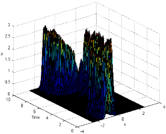
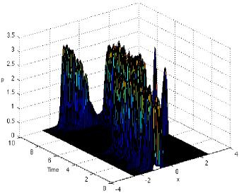
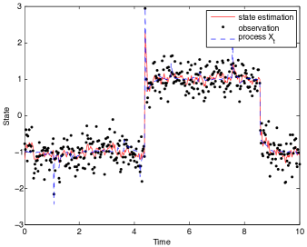
In Figures 1 and 2, we show the conditional density $p(x,t)$, together with the corresponding most probable orbit (taken as the state estimation for $X_{t}$), together with observations $y_{k}$ and a true state path $X_{t}$. The initial density is either Gaussian or uniform, but centered at the metastable state $-1$. Notice that the estimated state captures the transitions from $-1$ to $+1$ and then back to $-1$, during the time period $0<t<10$.

Figure 1: Example 1 – Conditional probability and state estimation when $\alpha=1.5$. The initial probability density is Gaussian centered at $-1$. Online version: The red curve in the right panel is the estimate state orbit (i.e., most probable orbit).

Figure 2: Example 1 – Conditional probability and state estimation when $\alpha=0.75$. The initial probability density is uniform on $(-1.25,-0.75)$. Online version: The red curve in the right panel is the estimate state orbit (i.e., most probable orbit).

3 Inferring transitions with continuous time observations

We consider the following scalar state system with a symmetric $\alpha-$stable Lévy motion

$$dX_{t}=f(X_{t},t)dt+dL_{t}^{\alpha},\;\;X_{0}=x,$$ (14)

together with a continuous time scalar observation system:

$$dY_{t}=h(X_{t},t)dt+dW_{t},\;\;Y_{0}=y,$$ (15)

where $h$ is a given vector field and $W_{t}$ is a Brownian motion.

The unnormalized conditional probability density $p(x,t|Y)$ satisfies a nonlocal Zakai equation ( [23, 13, 22]):

$$dp(x,t|Y)=A^{*}p(x,t|Y)\;dt+h(x,t)p(x,t|Y)\;dY_{t},$$ (16)

where $A^{*}$ is the adjoint operator of the generator $A$:

$$A^{*}\varphi = -(f(x,t)\varphi(x))^{{}^{\prime}}$$ (17)

$$+\int_{{\mathbb{R}}^{1}\setminus\{0\}}[\varphi(x+y)-\varphi(x)-I_{\{|y|<1\}}\;y\varphi^{\prime}(x)]\;\nu_{\alpha}({\rm d}y),$$

and $p(x,0|Y)$ is the initial density of $X_{t}$ (say a uniform distribution near the metastable state $-1$). The Zakai equation (16) may be numerically solved with a finite difference method based on [11, 12] together with a discretization of the noisy term at the current space-time point and $dY_{t}\approx Y_{t+\Delta t}-Y_{t}$. The initial probability density is taken either as a Gaussian distribution or a uniform distribution. For other numerical methods, see, for example, [18, 3, 17, 6, 31].

Remark 1.

The normalized conditional probability density $p(x,t\mid Y_{t})$ satisfies the nonlinear Kushner’s equation

$$dp(x,t\mid Y_{t}) =A^{*}p(x,t\mid Y_{t})dt+(h(x,t)-\hat{h}(x_{t},t))(dz_{t}-\hat{h}(x,t)dt)p(x,t\mid Y_{t})$$

$$=A^{*}p(x,t\mid Y_{t})dt+h(x,t)p(x,t\mid Y_{t})dz_{t}-h\hat{h}pdt-\hat{h}pdz_{t}+\hat{h}\hat{h}pdt,$$

where $\hat{h}(x_{t},t)$ is the mathematical expectation of $h(X_{t},t)$, with respect to $p$.

The conditional density $p(x,t|Y)$ provides information for the system evolution. With the observation, we can infer possible transitions from the metastable state $-1$ to the metastable state $+1$, within a time range $(0,T)$. If the system starts with a probability distribution $p_{0}(x)$ near the metastable state $x=-1$, then the conditional density $p(x,t|Y)$ helps us to infer whether the system will get near the other metastable state $+1$, and vice versa. This may be achieved by examining the most probable orbits for the system, under the observation. Define $x^{*}(x_{0},t)\triangleq\mbox{ maximizer for }\max_{x\in{\mathbb{R}}^{1}}p(x,t)$.
This provides the most probable orbit ([10, 7]) starting at $x_{0}$. We take this as our state estimation for $X_{t}$, as in [19].

Let us illustrate this by an example.

Example 2.

Let us consider the following scalar SDE state equation with a symmetric $\alpha-$stable Lévy motion:

$$dX_{t}=4(X_{t}-X_{t}^{3})dt+\sqrt{0.24}\;dL^{\alpha},\;\;X_{0}=x_{0}.$$

The scalar observation equation is given by

$$dY_{t}=X_{t}dt+\sqrt{0.05}\;dW_{t}$$

When noise is absent, the state system has two stable states: $-1$ and $+1$.

The corresponding nonlocal Zakai equation is solved by a finite difference scheme with space stepsize $\Delta x=0.05$ and time stepsize $\Delta t=0.001$.

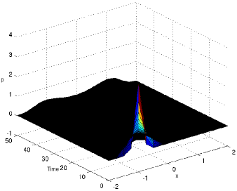
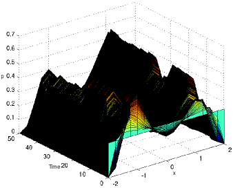
In Figures (3) - (4), we show the conditional density $p(x,t)$, together with the corresponding most probable orbit (taken as the state estimation for $X_{t}$), together with a true state path $X_{t}$. The initial density is either Gaussian or uniform, but centered at the metastable state $-1$. Notice that the estimated state captures the transitions from $-1$ to $+1$, then back to $-1$, and finally to $+1$, during the time period $0<t<50$.

Figure 3: Example 2 – Conditional probability (left) and state estimation (right) when $\alpha=1.5$. The initial probability density is Gaussian centered at $-1$.

Figure 4: Example 2 – Conditional probability (left) and state estimation (right) when $\alpha=1.5$. The initial probability density is uniform on $(-2,2)$.

References

• [1] N. U. Ahmed, Linear and Nonlinear Filtering for Engineers and Scientists. World Scientific, 1999.
• [2] D. Applebaum, Lรฉvy Processes and Stochastic Calculus. Cambridge University Press, Cambridge, UK, 2004.
• [3] A. Bain and D. Crisan, Fundamentals of Stochastic Filtering. Springer, New York, 2009.
• [4] J.ย Bertoin, Lรฉvy Processes, Cambridge University Press, Cambridge, U.K., 1998.
• [5] D. Brockmann, Human Mobility and Spatial Disease Dynamics, in Reviews of Nonlinear Dynamics and Complexity, Volume 2, 2009, pp.1 - 24. doi: 10.1002/9783527628001.ch1
• [6] Z. Cai, F. Le Gland and H. Zhang, An Adaptive Local Grid Refinement Method for Nonlinear Filtering. [Research Report] RR-2679, 1995.
• [7] Z. Cheng, J. Duan and L. Wang, Most probable dynamics of some nonlinear systems under noisy fluctuations. Commun. Nonlinear. Sci. Numer. Simulat, 30(2016)108-114.
• [8] P. D. Ditlevsen, Observation of ฮฑโˆ’limit-from๐›ผ\alpha-stable noise induced millennial climate changes from an ice record. Geophys. Res. Lett. 26 (1999), 1441-1444.
• [9] P. D. Ditlevsen, Anomalous jumping in a double-well potential. Phys. Rev. E 60 (1999), No. 1, 172-179.
• [10] J.ย Duan, An Introduction to Stochastic Dynamics, Cambridge University Press, New York, 2015.
• [11] T. Gao, J. Duan, X. Li and R. Song, Mean exit time and escape probability for dynamical systems driven by Lรฉvy noise. SIAM J. Sci. Comput. 36 (3) (2014) A887โ€“A906.
• [12] T. Gao, J. Duan and X. Li, Fokker-Planck equations for stochastic dynamical systems with symmetric Lรฉvy motions. Under revision with Applied Math and Comput., 2015.
• [13] B. Grigelionis and R. Mikulevicius, Nonlinear filtering equations for stochastic processes with jumps. In The Oxford handbook of nonlinear filtering, D. Crisan and B. L. Rozovskii (Eds.), Oxford University Press, p. 95-128, 2011.
• [14] N. E. Humphries, H. Weimerskirch, N. Queiroz E. J. Southall and D. W. Sims, Foraging success of biological Lรฉvy flights recorded in situ, Proc. Natl. Acad. Sci. 109(19):7169-7174 (2012).
• [15] A. Janicki and A. Weron, Simulation and Chaotic Behavior of ฮฑโˆ’limit-from๐›ผ\alpha-Stable Stochastic Processes, Marcel Dekker, Inc., 1994.
• [16] A. H. Jazwinski, Stochastic Processes and Filtering Theory. Academic Press, New York, 1970.
• [17] K. Law, A. Stuart and K. Zygalakis, Data Assimilation: A Mathematical Introduction. Springer, New York, (2015).
• [18] S. Lototsky, R. Mikulevicius and B. L. Rozovskii, Nonlinear Filtering Revisited: A Spectral Approach. SIAM Journal on Control and Optimization, 1997, Vol. 35, No. 2, pp. 435-461.
• [19] R. N. Miller, E. F. Carter, Jr and S. T. Blue, Data assimilation into nonlinear stochastic models Tellus (1999), 51A, 167ย–194.
• [20] B. Oksendal, Stochastic Differential Equations. Sixth Ed., Springer-Verlag, New York, 2003.
• [21] E. Olivieri and M. Eulalia Vares, Large Deviations and Metastability. Cambridge University Press, New York, 2004.
• [22] S. Popa and S. S. Sritharan, Nonlinear Filtering of Ito-Levy Stochastic Differential Equations with Continuous Observations. Communications on Stochastic Analysis, Vol. 3, No. 3, (2009), pp. 313-330.
• [23] H. Qiao and J. Duan, Nonlinear Filtering of Stochastic Dynamical Systems with Lรฉvy Noises. Adv. in Appl. Probab. Volume 47, Number 3 (2015), 902-918.
• [24] G. Samorodnitsky and M. S. Taqqu, Stable Non-Gaussian Random Processes, Chapman and Hall, 1994.
• [25] K.-I. Sato, Lรฉvy Processes and Infinitely Divisible Distributions, Cambridge University Press, Cambridge, 1999.
• [26] D. Schertzer, M. Larcheveque, J. Duan, V. Yanovsky and S. Lovejoy, Fractional Fokkerโ€“Planck equation for nonlinear stochastic differential equations driven by non-Gaussian Lรฉvy stable noises. J. Math. Phys., 42 (2001), 200-212.
• [27] M. F. Shlesinger, G. M. Zaslavsky and U. Frisch, Lรฉvy Flights and Related Topics in Physics (Lecture Notes in Physics, 450. Springer-Verlag, Berlin, 1995).
• [28] T. H. Solomon, E. R. Weeks, and H. L. Swinney, Observation of anomalous diffusion and Lรฉvy flights in a two-dimensional rotating flow. Phys. Rev. Lett. 71, 3975 - 3978 (1993).
• [29] W. A. Woyczynski, Lรฉvy processes in the physical sciences. In Lรฉvy Processes: Theory and Applications, O. E. Barndorff-Nielsen, T. Mikosch and S. I. Resnick (Eds.), 241-266, Birkhรคuser, Boston, 2001.
• [30] Z. Yang and J. Duan, An intermediate regime for exit phenomena driven by non-Gaussian Lรฉvy noises. Stochastics and Dynamics, Vol.8, No.3, 583-591, 2008.
• [31] S. Yau, New algorithem in real time solution of the nonlinear filtering problem. Communications in Information and Systems, Vol.8, No.3, 303-332, 2008.