Bayesian Social Influence in the Online Realm

Abstract

Our opinions, which things we like or dislike, depend on the opinions of those around us. Nowadays, we are influenced by the opinions of online strangers, expressed in comments and ratings on online platforms. Here, we perform novel “academic A/B testing” experiments with over 2,500 participants to measure the extent of that influence. In our experiments, the participants watch and evaluate videos on mirror proxies of YouTube and Vimeo. We control the comments and ratings that are shown underneath each of these videos. Our study shows that from 5$\%$ up to 40$\%$ of subjects adopt the majority opinion of strangers expressed in the comments. Using Bayes’ theorem, we derive a flexible and interpretable family of models of social influence, in which each individual forms posterior opinions stochastically following a logit model. The variants of our mixture model that maximize Akaike information criterion represent two sub-populations, i.e., non-influenceable and influenceable individuals. The prior opinions of the non-influenceable individuals are strongly correlated with the external opinions and have low standard error, whereas the prior opinions of influenceable individuals have high standard error and become correlated with the external opinions due to social influence. Our findings suggest that opinions are random variables updated via Bayes’ rule whose standard deviation is correlated with opinion influenceability. Based on these findings, we discuss how to hinder opinion manipulation and misinformation diffusion in the online realm.

This manuscript was compiled on

-2pt

In the previous century, experts heavily influenced the public opinion via mass media (1, 2). Nowadays, billions of individuals express their opinions in the online realm through online comments, reviews, and evaluations (3). Unfortunately, it is relatively easy and cheap to fake such online opinions, compared with physical world (4, 5). In the recent years, so-called astroturfers were hired to proliferate selected opinions and fake news online during major societal events, including democratic elections (6, 7). To design systems that are robust to misinformation and manipulation, it is crucial to uncover the extent and the mechanism of social influence.

The challenge in experimental studies of social influence is that traditional lab experiments (8, 9) and online surveys (10) lack external validity. Field experiments, on the other hand, yield less control over confounding factors, hindering causal inference (11, 12, 13, 14). To address these experimental challenges, we conduct novel academic A/B testing experiments. We create “clones” of existing social media websites, i.e., mirror proxies of real websites that are fully controlled by researchers to perform randomized experiments. These mirror proxies have exactly the same look and basic functionalities as their real counterparts. In our experiments, the participants watch and evaluate videos on YouTube and Vimeo, i.e., popular video-sharing platforms, in their private spaces and comfort zones. Underneath each of the videos, we show different types of social feedback, including the comments and the counters for views, likes, and dislikes. In our experimental conditions, we randomly modify this social feedback by suppressing some of the comments and lowering the counters. Then, we survey the participants about their opinions on each of the videos, to find whether the social feedback they are exposed to influences public opinion. The participants are unaware that this social feedback is modified, but they are informed that the goal of the experiments is to survey their opinions. Among others, we quantify the extent of social influence of online strangers on the opinions of participants and test whether the comments or the counters exert more influence. Thanks to our novel A/B testing setup, these measurements are precise and yield high external validity.

The results of social influence experiments are typically explained with the socio-psychological theories of informative and normative social influence (15, 16, 17). The former theory states that social influence stems from our need for accurate information about real world and that this influence is facilitated by the objective perceptual uncertainty about the stimulus. The theory of normative influence explains social impact with the need to be accepted by others, arising when a mutual relationship between individuals is present. However, social influence is observed even if these conditions are not met (18). Indeed, the participants of our experiments watch and evaluate videos that do not exhibit objective perceptual uncertainty and they are exposed to social signals from online strangers. The more recent theory of self-categorization addresses these points and explains the results of seminal experiments on social influence (9, 8) by introducing subjective uncertainty and arguing that social signals interfere with that uncertainty in a way that informative and normative needs are inseparable (18). Human judgments under uncertainty have been extensively studied in psychology (19, 20, 21, 22). Pioneering works in this area measure human biases in probabilistic reasoning by means of comparisons with Bayesian inference, in particular the binomial model (23, 19, 24, 22). Here, we derive the corresponding binomial model of social influence from basic principles of probability theory, following empirical Bayes method. In our settings, priors and posterior distributions are unknown and estimated from observations. With this model, we measure social influenceability and its relation to uncertainty in online social media and introduce a Bayesian theory of social influence.

Results

Table 1: Summary of the experiments.

	Experiment I	Experiment II
Platforms:	YouTube, Vimeo	YouTube
Participants:	1,116	1,391
Videos:	8	14
Experimental conditions:	11	7
Expressed opinions:	8,928	9,737
Opinion scale:	5-point Likert	200-point bipolar
Comment tracking:	No	Yes

In total, over 2,500 subjects participated in our experiments (Table 1). The participants were recruited and compensated via Amazon Mechanical Turk (25). Each participant of our online experiments is instructed, in one sitting, to watch several videos, familiarize themself with social feedback to these videos, and answer whether they like the video. Each web page, showing a video with corresponding user comments, is a clone of an existing web page on YouTube or Vimeo. The videos are on a variety of topics, ranging from pranks and commercial ads to societal issues and innovations. We selected videos that had up to a million views at the moment of data gathering, but not more, to avoid potential confounding effects from participants who have seen them before. Albeit the videos were pre-selected, many participants of our experiments found them to be entertaining. Over 185 participants used words “great”, “fun”, or “enjoy” in reference to the videos and the experiment in an optional text-box comment presented at the end of each experiment (see Demographics and Feedback of Participants in SI Appendix).

Our goal is to measure how social feedback influences opinion. Each video comes with two types of social feedback: i) the comments of its prior viewers and ii) the counters for views, thumbs up, and thumbs down (see Figure 1). In the experimental conditions, we control and modify these two types of social feedback. In the negative experimental conditions, we hide positive comments and lower the numbers of views and thumbs up; whereas in the positive conditions, we make the modifications that are exactly opposite. Overall, in the experiments there are three main negative conditions and three main positive conditions, differing in the degree of modifications to social feedback. As the control condition we take the respective video with its original unmodified comments and the values of counters.

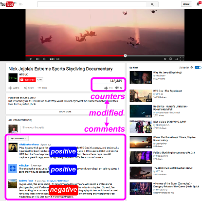
Figure 1: An illustration of the experiments. The comments are labeled as positive or negative towards the video before the experiments. Under experimental conditions, some of the comments are randomly suppressed and the counters for views and for thumbs up and down are modified.

Figure 2: The probability of a positive opinion under the control condition (circle) and the experimental conditions of various strength (squares and stars). The color of markers corresponds to positive (blue) and negative (red) conditions. This result is averaged over all videos and experiments. The $95\%$ confidence intervals are from BCA bootstrap. (A) Main experimental condition. (B) Partial experimental conditions in which either comments or counters (diamonds) or both (stars) are modified.

Then, we compute the probability of positive opinion about any video, $P_{+}$, as the fraction of positive answers across users and videos in the given experimental condition. This probability increases monotonously with the extent of modification of social feedback, ordered from the most negative to the most positive main experimental condition (Figure 2A). In other words, the more positive comments, thumbs up, and views a participant sees under a video, the more likely they are to have a positive opinion about that video. The $95\%$ confidence intervals show that the difference in the probability of positive opinion between experimental conditions is statistically significant for most of the condition pairs. Comparisons of the distributions of raw responses confirm this result. For instance, there is a statistically significant difference in opinions between the control condition and the strongly positive and negative conditions (Mann-Whitney U test, $p<10^{-17}$ and $p<10^{-4}$, respectively). We conclude that the opinions are influenced by social feedback both positively and negatively (14).

In addition to opinion, we also survey the participants about their willingness to share the video they watched with friends. The willingness to share a video is correlated with the opinion about that video, because positive opinion about an object creates incentives for sharing it with friends (26). We find that all presented results are qualitatively and often quantitatively the same for the opinion and the sharing willingness, under different psychometric scales (see Experiment I and Experiment II in SI Appendix).

So far we have shown the result for the main experimental conditions, in which both the comments and the counters are modified. However, it is not clear whether the participants are influenced by the comments or the counters. To answer this question, in Experiment I, we measure which type of social feedback exerts more influence on the opinions: the comments or the counters? To this end, additional experimental conditions are introduced, in which either only comments or only counters are modified, i.e., two positive and two negative partial experimental conditions.

In contrast to main positive and negative conditions, the partial conditions modify only one type of social feedback, instead of both of them. We find that the probability of positive opinion is influenced more by the modifications of comments than the counters (compare the diamonds of the same color in Figure 2B). In other words, the comments have larger impact on opinion than the thumbs and views. The comments significantly influence the opinion in negative and positive experimental conditions with respect to the original condition ($p=0.0002$ and $p=0.02$, respectively), whereas the influence of thumbs is insignificant.

In the remainder, we explain the mechanism of social influence by analyzing in more detail the influence of comments on public opinion. In Experiment II, to better understand the mechanism of social influence, we make more precise measurements for more videos and participants, while tracking which comments were read by each of the subjects. We exploit this information to measure how the probability of a positive opinion about a video, $P_{+}$, depends on the difference, $\Delta n$, in the number of positive and negative comments read by a participant (Figure 3). Subjects have a relatively positive opinion about a given video when positive comments prevail among the comments that they read ($\Delta n>>0$), and a relatively negative opinion if negative comments prevail ($\Delta n<<0$). For each of the videos, the probability of positive opinion $P_{+}(\Delta n)$ saturates at a lower value when $\Delta n$ is very negative and at a higher value when $\Delta n$ is very positive. For most videos, the probability $P_{+}(\Delta n)$ has a sigmoid shape and is anti-symmetric, exposing a systematic dependence. Next, we use a Bayesian theory and models of social influence, to explain these experimental results and to estimate the percentage of individuals influenced by the comments.

Figure 3: Public opinion about a video depends on majority opinion in comments. The probability of positive opinion is plotted versus the difference in the number of positive and negative comments read by a subject. Magenta points correspond to the moving average over $100$ measurements. The model applied to the finite real data expects the running average in the gray area marking $99\%$ confidence interval. The black line is the model applied to an infinite data.

Prior works proposed models of social influence that are accurate at predicting opinions in specific circumstances (12, 13, 14). In this study, we explain the mechanism of social influence with a generic Bayesian theory. This theory posits that opinions are hypotheses whose probabilities of being correct are updated in the process of social influence, following Bayes’ theorem. To this end, we assume that social signals serve as evidence validating corresponding opinions. This assumption is equivalent to the basic assumption of the self-categorization theory that agreement with others “subjectively validates our responses [i.e., opinions] as veridical reflections of the external world” (18). To make a direct correspondence to Bayesian estimation, we distinguish between prior and posterior opinions, i.e., latent parameters representing the opinions before and after social influence, respectively. In particular, using this Bayesian theory, we derive the posterior probability of an individual to express a positive opinion, $P_{+}$, as a simple logit model, which accounts for the prior opinion of the individual and the opinions expressed by others (27, 28). On the grounds of this generic theory, other models could be proposed as well, but the logit model is particularly simple and sufficiently expressive. The results of our Experiment II are explained by a mixture of logit models, corresponding to the mixture of participants. We explore many variants of this mixture model, which differ in the number of components, using Akaike information criterion. The best models reveal interesting common properties.

The logit model is derived as a result of Bayesian estimation under social feedback only when, instead of purely rational decisions (29, 30), individuals respond with an additional stochastic component known as probability matching, as shown across animal species, including humans (28, 27, 10, 31) (see Derivation of Logit Model in SI Appendix). Under this model, the posterior probability of a positive opinion is $P_{+}(\Delta n,s,a)=1/\left(1+\exp(-s\Delta n-a)\right)$. Here, $a$ is the latent parameter representing the prior opinion of an individual, which corresponds to personal memories and thoughts on a given subject, and $s$ is their influenceability, which describes how strongly influenced they are by the social feedback on that subject. This model predicts that the posterior probability of expressing a positive opinion in a homogenous population, where all individuals have the same value of parameters $a$ and $s$, tends to saturate at $0$ and $1$ for $\Delta n<<0$ and $\Delta n>>0$, respectively. This phenomena is not observed in our experimental data, likely because each individual reacts differently to social influence on a given topic. To include this heterogeneity in the model, we treat the overall population as a mixture of heterogeneous individuals, that is, a mixture of logit models. Each component of the mixture correspond to a sub-population of individuals. A sub-population $k$ is characterized by the fraction $p_{k}$ of individuals belonging to it, their prior opinion $a_{k}$, and their influenceability $s_{k}$. However, we do not know how many sub-populations there exist and whether their parameters differ between videos or are necessary for explaining the data. To answer these questions, we explore thousands of variants of the sub-population model, differing in the number of sub-populations and parameters. First, we consider variants having from one ($K=1$) to six ($K=6$) sub-populations. Second, each of the parameters, $a_{k}$,$s_{k}$, and $p_{k}$, either depends on the video, is constant across videos, or vanishes due to replacement by a neutral constant. We fit each unique variant of this model to the data by maximizing the likelihood of our observations. To obtain the model that best explains our data, we rank these models by Akaike information criterion (32).

We then analyze what the best models share in common. The top four models have two sub-populations: a non-influenceable sub-population with $s_{1}=0$ and an influenceable sub-population with the influenceability $s_{2}>0$, both of which are constant across videos (see Model Selection in SI Appendix). The top model fits the data remarkably well (Figure 3). It has $s_{2}=0.8\pm 0.005$ across videos, whereas the other parameters, namely $p_{1}$, $a_{1}$, and $a_{2}$, depend on videos. The fraction of influenced individuals varies from $p_{2}=0.05\pm 0.05$ to $p_{2}=0.40\pm 0.05$, depending on the video (see The Parameters of the Best Model in SI Appendix), which means that a large portion of individuals is influenced by the comments they read. Possibly, the participants are influenced by the comments, because they agree with them. To test this hypothesis, we measure whether the membership in the influenceable sub-population is related to the agreement with comments, self-reported by each participant for each video. The membership of a sample in a sub-population generally depends on the likelihood that this sample was generated by that sub-population, i.e., $P_{+}(\Delta n,s_{k},a_{k})$. This likelihood is significantly correlated with the agreement with comments (Spearman’s $\rho=0.41$, $p<10^{-99}$). We conclude that social feedback tends to influence the opinion of subjects who agree with the exposed opinions, although it can arise without a conscious agreement as well.

Apart from the difference in influenceability, there are other notable distinctions between the two sub-populations. First, the prior opinion of the influenceable sub-population has a significantly larger standard error in comparison with the non-influenceable sub-population. After correcting for the difference in sizes of the two sub-populations, with the factor $\sqrt{p_{2}/p_{1}}$, we find that the standard error of prior opinion of an influenceable individual is from $2$ to $31$ times larger than of a non-influenceable individual (depending on the video, as shown in Figure 4)A. Prior work shows that the standard error of a perceived variable is closely and inversely related to the confidence of human decisions depending on that variable (21). Thus, our result suggests that influenceable individuals are more uncertain in their prior opinions than non-influenceable individuals, making them more influenceable. This result is in line with the expectations of the self-categorization theory. Second, we find that the prior opinions of non-influenceable sub-population, $a_{1}$, are strongly correlated with the external opinions ($p<10^{-4}$, the leftmost bar in Figure 5)B. In contrast, the prior opinions of influenceable sub-population, $a_{2}$, are not correlated with the external opinions (the gray bar in Figure 5)B and become correlated only after being socially influenced (the two middle bars in Figure 5)B. In other words, social influence helps to develop weak opinions with high standard error into stronger opinions with lower standard error that are closer to the external opinions. However, under strongly modified experimental conditions, the posterior opinions of influenceable sub-population become heavily distorted and further from the external opinions than their prior opinions (the rightmost bar in Figure 5)B. This result shows that the influenceable individuals are vulnerable to opinion manipulation.

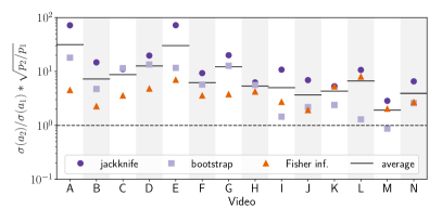
Figure 4: The ratio of standard error of prior opinion of the influenceable and non-influenceable individuals. Each black horizontal line is an average over three methods of estimating standard error: as the inverse of observed Fisher information (triangles) or via jackknife resampling (circles) or bootstrap resampling (squares).

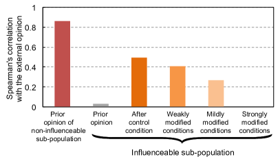
Figure 5: The average correlation between the external opinion about videos and the prior and posterior opinions of either non-influenceable or influenceable individuals. As the external opinion we take the fraction of thumbs up for the original video (reported in Table S2 in SI Appendix). As the socially influenced, i.e., posterior, opinions we take the prior opinion on videos plus the effect of social influence, i.e., $a_{v}+s_{2}\Delta n$, where $\Delta n$ is a sample for a random individual for the given video in the experimental conditions of the given kind. The correlation is computed over videos and averaged over the samples.

Discussion

Our findings provide empirical support for the probabilistic nature of opinion formation in three different ways. First, in the Bayesian theory of social influence, the prior opinion is updated due to social feedback via Bayes’ rule, giving the posterior distribution of opinion (29, 30). The view of social influence, as a social validation of opinions, is consistent with self-categorization theory. Additionally, the theory of self-categorization states that the influence is greater among individuals who share salient identities. The question of whether there is a natural counterpart of this mechanism in Bayesian statistics is open for future research. Second, the logit model explains our experimental observations only if we apply as the decision rule so-called probability matching, which means that the expressed opinions are drawn from the posterior distribution of opinion (27, 28). Third, our findings suggest that the prior opinion is also a random variable whose variance is correlated with influenceability. One can interpret the standard error of prior opinion as its standard deviation. Then, the prior opinions with larger variance tend to be more influenceable, whereas the prior opinions with lower variance are less influenceable. On the grounds of Bayesian statistics, it is expected that weak priors are affected more by observations than strong priors, when forming posteriors, in agreement with our measurements and the prediction of self-categorization theory that the uncertainty facilitates influence. Note, however, that while this third point is naturally explained on the grounds of Bayesian statistics, the logit model captures it only indirectly through the components of the mixture. In future works, the variance of prior opinions can be modeled with hierarchical Bayesian models and estimated with empirical Bayes methods. Our Bayesian theory of social influence provides a base for the development of such alternative models. The theory posits that social influence is a Bayesian updating of prior opinions due to observed social feedback, possibly as a part of generic distributed Bayesian inference about the structure of reality (33, 34).

Opinion manipulation and misinformation are particularly pervasive (6, 7) and nearly effortless in online platforms, which nowadays have billions of users and become crucial for the stability of society (3, 35). Further research is indispensable to prevent the abuse of social computing systems and to form a more robust society. Bayesian social influence allows individuals with weak prior opinions to form more informed opinions, by the virtue of expert influence on a given topic. However, these individuals are also vulnerable to opinion manipulation, for instance via astroturfing, i.e., paid campaigns created to influence individuals without their awareness. In other words, there are both good and bad effects of social influence. Our measurements of social influence yield high external validity, because our A/B testing experiments are conducted on clones of existing social media websites. Our findings suggest that randomized experiments in conjunction with statistical modeling of social influence can be used to detect vulnerable users and protect them from opinion manipulation and misinformation. Note that online platforms, such as YouTube and Facebook, routinely perform such randomized experiments for other commercial purposes. Social computing systems could be designed to emphasize the good influence and hinder the bad influence by detecting and protecting vulnerable users, and by estimating and exposing the expertise of its users within topical domains. Although we anticipate that both domain vulnerability and expertise are related to influenceability within that domain, we point out that subsystems for measuring vulnerability and expertise shall evolve over years through an open scientific process, because of their importance to society. Nowadays, online ratings and comments are simple and heavily affected by sampling bias, i.e., a piece of content is judged by a biased sub-sample of population and there is no way to see how other sub-populations would judge that content. Future social computing systems could characterize the people who evaluate a given piece of content, correct for the sampling bias in ratings and comments, and provide information about how experts evaluate that content. These systems would hinder opinion manipulation and the diffusion of fake news, by informing users, the vulnerable ones in particular, about the nature of ratings and comments they see.

Methods

Comments underneath videos. Before the experiments, from one (Experiment I) to three (Experiment II) editors label each of the comments as either positive, negative, or neutral towards the respective video. There is a significant agreement between the three labelers (Fleiss’ kappa of $0.56$). The comments are always shown to participants in the reverse chronological order of their original creation date, reflecting the default setting in the respective video-sharing platforms at the time when the experiments were performed.

Experimental conditions. Each participant watches in a randomized order the same set of videos randomly assigned to the experimental or control conditions. In the case when the total number of experimental conditions is different than the number of videos, we perform a round-robin over experimental conditions to ensure a balanced assignment of conditions to videos across participants.

Psychometric scales. To take robust and precise measurements, we use different psychometric scales for surveying opinions in the two experiments. The participants express their opinions about a video by declaring their agreement with the statement “I like this video”. In Experiment I, the participants respond to this question on a standard 5-point Likert scale, ranging from “Strongly disagree” to “Strongly agree”. In Experiment II, we use a more precise 200-point scale that ranges from 100% “Disagree” to 100% “Agree” (36). For the sake of simplicity, in the analysis we treat all “Agree” answers as positive opinion and all “Disagree” answers as negative opinion, independently whether they correspond to “Weakly agree”, “Strongly Agree”, “5% Agree”, or “75% Agree”.

The binomial model with decisions copying hypotheses. The derivation of the model follows the steps of Perez-Escudero et al. (27), however, its new framing makes a more explicit connection to Bayesian inference, by formalizing posterior predictive probability and likelihood, and is adapted to the setting of opinion formation. The derivation makes a series of simplifying assumptions, but each of them can be relaxed, as we demonstrate in the following subsections introducing other models based on the same Bayesian principles.

We consider an action of liking or disliking a video as a reflection of hypotheses, $\theta$, considered by the focal individual, referred to as ego as a distinction from other individuals. Under the binomial model, we assume that ego considers the minimal number of only two hypotheses, e.g., the video is good ($\theta_{+}$) or bad ($\theta_{-}$). Ego estimates their posterior probability of each hypothesis, or posterior opinion, using their prior information about these hypotheses, $P(\theta)$, and the relevant observed social signals, $B$, with which they update their prior probability and obtain the posterior probability of hypotheses, $P(\theta|B)$, following Bayes’ rule

$$P(\theta|B)=\frac{P(B|\theta)P(\theta)}{P(B)}.$$ (1)

Since only two hypotheses are considered, it is useful to write Bayes’ theorem in its posterior-odds form, that is

$$\frac{P(\theta_{+}|B)}{P(\theta_{-}|B)}=\frac{P(B|\theta_{+})P(\theta_{+})}{P(B|\theta_{-})P(\theta_{-})}.$$ (2)

Next, we assume that ego estimates $P(B|\theta)$ by naively assuming that the observed opinions are independent of each other. This assumption has been shown to be a good approximation of the model including dependencies for animals (27). Under this assumption $P(B|\theta)=Z\prod_{i=1}^{N}P(b_{i}|\theta)$, where $B$ is the set of $N$ comments read by ego and $b_{i}$ is the opinion expressed in the comment $i$. $Z$ is a normalization constant ensuring $\sum_{B}P(B|\theta)=1$, also know as partition function, which is a combinatorial term counting the number of possible comment sequences for the set of comments $B$. As in the design of our experiments, we assume that each comment can be categorized as positive ($b_{+}$), negative ($b_{-}$), or neutral ($b_{=}$), totaling $N=n_{+}+n_{-}+n_{=}$ comments. Then,

$$P(B|\theta)=ZP(b_{+}|\theta)^{n_{+}}P(b_{-}|\theta)^{n_{-}}P(b_{=}|\theta)^{n_{=}}.$$ (3)

We assume that neutral comments do not add any information about the correctness of hypotheses, $P(b_{=}|\theta_{-})=P(b_{=}|\theta_{+})$, and we will neglect them in the reminder for simplicity. Inputting the last two formulas to Equation 2 gives

$$\frac{P(\theta_{+}|B)}{P(\theta_{-}|B)}=\frac{P(b_{+}|\theta_{+})^{n_{+}}P(b_{-}|\theta_{+})^{n_{-}}P(\theta_{+})}{P(b_{+}|\theta_{-})^{n_{+}}P(b_{-}|\theta_{-})^{n_{-}}P(\theta_{-})}.$$ (4)

Note that $P(\theta_{-}|B)=1-P(\theta_{+}|B)$ and the logarithm of this equation gives the log-odds

$$\log\frac{P(\theta_{+}|B)}{1-P(\theta_{+}|B)}=n_{+}s_{+}+n_{-}s_{-}+a,$$ (5)

where $s_{+}=\log\frac{P(b_{+}|\theta_{+})}{P(b_{+}|\theta_{-})}$, $s_{-}=\log\frac{1-P(b_{+}|\theta_{+})}{1-P(b_{+}|\theta_{-})}$, and $a=\log\frac{P(\theta_{+})}{P(\theta_{-})}$. The parameter $a$ captures the relative prior probability of the two hypotheses, i.e., the relative prior opinion of ego, whereas $s$ determines how much is the prior opinion affected by the observed social signals. This formula for log-odds is further simplified, if we assume a symmetric influence of positive and negative comments, i.e., if $s_{+}=-s_{-}=s$, then a positive comment negates a negative comment. We recognize that the log-odds in Equation 5 are a linear function of the observed $n_{+}$ and $n_{-}$, so its parameters $s$, and $a$ can be estimated with a logistic regression model

$$P(\theta_{+}|B)=\sigma(s\Delta n+a),$$ (6)

where $n=n_{+}-n_{-}$ and $\sigma$ is a logistic function, but we still need to relate this posterior probability of hypotheses to the opinions expressed by ego.

So far we have considered the perceptual stage of decision-making, in which ego estimates which of the hypotheses is correct. Whether the video is liked or not is decided by a decision rule. Evidence for animals and humans suggests that individuals use a decision rule called probability matching (37, 38, 39, 27, 28). According to this rule, the ego expresses an opinion, $b$, by directly drawing the corresponding hypothesis from the posterior distribution of hypotheses, i.e.,

$$P(b=b_{+}|B)=P(\theta_{+}|B).$$ (7)

This decision rule is equivalent to the typical rule that future observations are draws from the posterior predictive distribution, that is the likelihood averaged over the posterior

$$P(b=b_{+}|B) =\sum_{\theta\in\{\theta_{+},\theta_{-}\}}P(b=b_{+}|\theta)P(\theta|B),$$ (8)

if only there is one-to-one mapping between $b$ and $\theta$ and samples of $b$ from the likelihood are copies of the draws from the corresponding posterior distribution of $\theta$, i.e., $P(b|\theta)=1$ if $b=b_{+}$ and $\theta=\theta_{+}$ or $b=b_{-}$ and $\theta=\theta_{-}$; otherwise $P(b|\theta)=0$. Thus, there is a direct mapping between hypotheses and expressed opinions; the difference between the two is that expressed opinions are drawn at random at the moment of an observation, whereas hypotheses are latent opinions that are not observed directly until they are copied and expressed. Finally, note that when ego is deciding what opinion to express (Equation 7), the likelihood function copies a draw from the posterior of ego; however, when the individuals whose opinions are observed by the ego are making a decision (Equation 3), then the likelihood function copies a draw from their own distributions over hypotheses, which ego aims to estimate with the parameter $s$.

Model fitting. The parameters of a mixture of logit models can be inferred with the expectation-maximization algorithm, but this approach gets stuck in local optima (44). Thus, we use a different, approximate, method for inferring the parameters of each model. Namely, we treat each individual as indistinguishable and estimate the probability of positive opinion as $P_{+}(\Delta n)=\sum_{k=1}^{K}p_{k}P_{+}(\Delta n,s_{k},a_{k})$, where $p_{k}$ is the fraction of individuals in the sub-population $k$ and $K$ is the total number of sub-populations. This probability does not depend on any particular individual, but instead it averages the probability of positive opinion over all individuals.

The parameters of a mixture of logit models can be inferred with the expectation-maximization algorithm, but this approach gets trapped in local optima (44). Thus, here we use a mean-field approximation of that model to find optimal values of parameters. Namely, we assume that individuals are indistinguishable. In such case, the probability that an unidentifiable individual from the whole population has a positive opinion about the video is

$$P_{+}(\Delta n)=\sum_{k=1}^{K}p_{k}\frac{1}{1+\exp(-s_{k}\Delta n-a_{k})},$$ (9)

where $p_{k}$ is the portion of individuals in sub-population $k$. The joint probability of observing opinions $\boldsymbol{y}$, given that the individuals were exposed to $\boldsymbol{\Delta}n$ comments is

$$\begin{split}L&=\prod_{u=1}^{U}\prod_{v=1}^{V}\left(P_{+}\left(\Delta n_{uv}\right)\right)^{y_{uv}}\left(1-P_{+}\left(\Delta n_{u}\right)\right)^{1-y_{uv}}\end{split}$$ (10)

where $U$ is the total number of individuals and $V$ is the total number of videos, and ${\sum_{k}p_{kv}=1}$ for each video $v$. To fit the parameters of this model, we maximize the log-likelihood $\log(L)$. We present detailed results of this fitting in the following subsections.

Standard errors of parameters. The standard error of each estimated parameter are obtained using three different methods. The first two methods correspond to random re-sampling of results among individuals: either via bootstrapping or jackknife approach. In the bootstrapping approach, we sample the results of experiment with replacements to obtain the same number of samples, that is individuals, as in the original experiment. Then, we fit the parameters of the model using such re-sampled data. We repeat this procedure $1000$ times and compute the standard error of the estimated parameters. The jackknife approach follows the same procedure, except that instead of sampling, we randomly drop one sample from the set of original results of the experiment. The third method of computing standard error is based on the analysis of the log-likelihood. We note that the covariance matrix of the estimated parameters $\hat{\theta}$ is an inverse of the observed Fisher information (negated Hessian of log-likelihood):

$$\boldsymbol{\Sigma}(\hat{\theta})=\left[\boldsymbol{\mathcal{I}}(\hat{\theta})\right]^{-1}=\left[-\frac{\partial^{2}\left(\log\left(P\left(\boldsymbol{\Delta n},\boldsymbol{y}|\theta\right)\right)\right)}{\partial\theta_{i}\partial\theta_{j}}\bigg{|}_{\theta=\hat{\theta}}\right]^{-1}.$$ (11)

Thus, the standard error of an estimated parameter $\hat{\theta}_{k}$ is the square root of the corresponding diagonal element of $\boldsymbol{\Sigma}(\hat{\theta})$. We compute the standard error for each parameter using this method and report it in the main text.

Some of the parameters differ considerably between videos, especially the prior opinions $a_{k}$ about the videos. Interestingly, the prior opinion of the non-influenceable sub-population about a given video takes similar values in various top models, whereas the prior opinion of influenceable sub-population varies largely across top models. Also, the standard error of the prior opinions is many times larger for the influenceable than non-influenceable sub-population. This difference may arise due to the fact that the non-influenceable sub-population is larger than influenceable sub-population. If we interpret the prior opinion $a_{k}$ of sub-population $k$ as a mean over prior opinions $a_{ku}$ of individuals belonging to this sub-population, then the standard error of this mean is $\sigma(a_{k})=\sigma(a_{ku})/\sqrt{U_{k}}$, where $U_{k}$ is the number of individuals belonging to that sub-population. Thus, to compare the standard errors of this parameter for the two sub-populations, we shall compute the ratio

$$\frac{\sigma(a_{2u})}{\sigma(a_{1u})}=\frac{\sigma(a_{2})\sqrt{U_{2}}}{\sigma(a_{1})\sqrt{U_{1}}}=\frac{\sigma(a_{2})\sqrt{p_{2}}}{\sigma(a_{1})\sqrt{p_{1}}},$$ (12)

where $p_{k}$ is the fraction of individuals belonging to the sub-population $k$. This ratio compares the intrinsic standard deviations of prior opinion of individuals belonging to two different sub-populations, taking into account that they differ in size.

Confidence intervals of the running probability. For the purpose of the presentation, we compute running probability of positive opinion about a video. Namely, given a set of answers $y$ from different users for specific $\Delta n$, we compute running probability of positive opinion with a sliding window of $n$ data points. To compute this running probability, the set of answers $y$ is ordered in the increasing order of $\Delta n$. Then, for every i-th window of $n$ experimental points we compute $\overline{\Delta n_{i}}=\frac{1}{n}\sum_{u=1}^{n}\Delta n_{u+i-1}$ and $P_{+,i,j}=\frac{1}{n}\sum_{u=1}^{n}y_{u+i-1}$. In our dataset, for a given value of $\Delta n$ usually there are several answers from different participants for which $\Delta n$ is the same. Note that the answers for a given $\Delta n$ do not have a natural order. To avoid any artifacts in the computation of the running probability due to the lack of order in the answers for a given $\Delta n$, we randomly permute the answers for that $\Delta n$ and compute $P_{+,i,j}$, where $j$ stands for that permutation. We repeat this process $m$ times to obtain the final running probability of positive opinion as an average over $m$ permutations, i.e., $\overline{P_{+,i}}=\frac{1}{m}\sum_{j=1}^{m}P_{+,i,j}$.

To show how well the model predicts the experimental probability, we compute the $99\%$ confidence interval of the model for the running probability. To this end, we calculate the running probabilities based on the artificial data simulated with the fitted model for the real finite set of $\Delta n$. We repeat this procedure $1000$ times to obtain $99\%$ confidence intervals of the model for each $\overline{\Delta n_{i}}$. We present these confidence intervals in Figure 1 of the main text and all other figures of running probability.

We thank Luis Fernandez Lafuerza for insightful discussions and feedback, Karin Chellew for her suggestions on the design of the experiments, Maria Cano-Colino for her help with comment labeling, and Manuel Gomez-Rodriguez for his comments on model learning. We acknowledge funding from the Volkswagen Foundation (P.A.G.), the Alexander von Humboldt Foundation (F.B.), the Fundação de Amparo à Pesquisa de Minas Gerais (F.B.), the Fundação para a Ciência e Tecnologia PTDC/NEU-SCC/0948/2014 (G.G.d.P.), and the Champalimaud Foundation (G.G.d.P.).

Supporting Information Appendix

Contents

1. 1 Experiment I
   1. 1.1 Description
   2. 1.2 Videos
   3. 1.3 Comments
   4. 1.4 Data Processing
   5. 1.5 Main Experimental Conditions
   6. 1.6 Partial Experimental Conditions
   7. 1.7 Results
   8. 1.8 Demographics of Participants
2. 2 Experiment II
   1. 2.1 Description
   2. 2.2 Videos
   3. 2.3 Comments
   4. 2.4 Data Processing
   5. 2.5 Demographics and Feedback of Participants
3. 3 Models
   1. 3.1 Model Selection
   2. 3.2 Parameters of the Best Model

1 Experiment I

We first conducted Experiment I, in preparation to Experiment II. To each participant, we showed videos with corresponding social feedback from two video-sharing websites, i.e., YouTube and Vimeo. We asked the participants what is their opinion about each of the videos. In Experiment I, we used a 5-point Likert scale to measure the opinion and we introduced partially manipulated conditions in which we altered either only comments or only the counters for thumbs and views. Here, we present a detailed description of this experiment and its results.

1.1 Description

Figure S6: Instructions given before starting the survey.

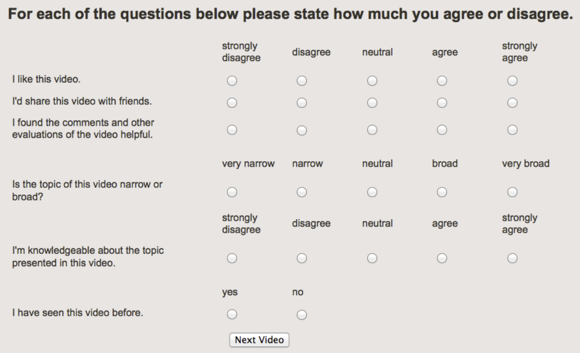
Figure S7: The survey performed immediately after the participant watched the video.

Before starting the survey the participants are given the instructions (nearly identical for both experiments, Figure S6). The subjects are asked to click on the image to watch the video, see the feedback of other people, and to evaluate the video. For each video, we ask a set of questions about the video (Figure S7). The participant can see the questions before watching the video, but cannot answer them without playing the video first, and all questions must be answered before advancing to the next video. The pages with the videos look exactly like in the original systems, i.e., in Youtube and Vimeo, except the social feedback to the videos is modified to various extent under different experimental conditions. The comments are shown under videos in the reverse chronological order of their original creation date, reflecting the default setting in the respective video-sharing platforms at the time when the experiments were performed.

For each video we conduct a survey (Figure S7). We ask the participant on a $5$-point Likert scale if she agrees with the statement evaluating her opinion about the video (“I like this video”) and her willingness to share the video (“I’d share this video with friends”). Additionally, we ask if the person saw this video before. In the analysis, we discard the responses which were influenced by the past exposures to the given video.

1.2 Videos

		Comments			Thumbs
Platform	Video	Pos.	Neut.	Neg.	Up	Down	Views	Link to the original
	HTC add	17	30	47	110	31	147,273	dwGGdM3Nj08
YouTube	Lamborghini	14	1	5	41	28	76,675	Pc7XHHCjtJI
	A girl singing	37	15	37	663	525	120,938	5JKJhY15NNA
	Supermarket joke	5	3	15	60	45	25,892	VqGaHxC3Zbg
	Google joke	2	7	10	50	-	-	9261909
Vimeo	Stride add	8	8	3	221	-	-	23061242
	Ipad skateboard	33	14	13	842	-	-	11480457
	Curing cancer	19	10	8	695	-	-	54668275

Table S2: Basic statistics of the original (non-manipulated) videos: the number of comments of various types, the number of thumbs up and thumbs down, and the number of views at the time of their collection (January 2014).

For the experiments, we picked four videos from YouTube and four videos from Vimeo. To avoid videos that subjects have seen before, we chose videos that have a public appeal but are not very popular, namely have from $20,000$ to $1$ million views, more than 15 comments (including some positive and negative ones), and over 15 thumbs. The links to the original videos and the numbers of comments, thumbs, and views for each of the videos are listed in Table S2. The average duration of videos is $104$ seconds. During the experiment each participant is shown all eight videos in a random order, each of them under a different experimental condition, chosen in a round-robin fashion from: the control condition, two strongly modified conditions, two mild conditions, two weak conditions, and four partial manipulations. We describe the experimental conditions below.

1.3 Comments

Each of the comments was labeled by an author as either positive, neutral, negative, or unreadable (see Table S2 for a summary). Positive comments are the comments that describe the video in a positive way, while negative comments are negative toward some aspects of the video. Neutral comments are mostly off-topic or do not contain any evaluations of the content of the video. The comments that are unreadable or are written in a language different from English are filtered out.

1.4 Data Processing

Before analyzing the data, we clean and filter it. Namely, we discard all answers that are incomplete due to technical reasons or individual mistakes, as well as double answers from the same participant (in total, we discard less than $6\%$ of all participants). To estimate the quality of answers, we measure how much time it takes for each participant to evaluate each video. We exploit this information, to invalidate the video evaluations that took a subject less time than half of video duration. Furthermore, we also invalidate the evaluations of videos that have been seen by the participant externally before the experiment, according to self-reports of participants for each video. Then, we discard the participants with answers invalidated for more than one videos. In total, we discard less than $10\%$ of all participants.

1.5 Main Experimental Conditions

The main experimental conditions include the control condition, two strongly modified conditions, two mild conditions, and two weak conditions. In strongly modified positive (negative) condition, we hide all negative (positive) comments, we show all neutral and positive (negative) comments, and we increase (decrease) the numbers of thumbs up and views by the factor of $10$. The mildly and weakly modified conditions are implemented as m-factor manipulations, which fine-tune the extent of modifications with respect to the control condition. In the m-factor positive (negative) manipulation, we hide all negative (positive) comments except randomly chosen $1/m$ comments, and multiply (divide) the numbers of thumbs up and views by the factor $m$. The mild conditions are $6$-factor manipulations, whereas the weak conditions are $3$-factor manipulations. Note that the aforementioned strongly modified conditions correspond to $10$-factor manipulations, except all comments of certain type are hidden instead of their majority.

1.6 Partial Experimental Conditions

We introduce partial experimental conditions to find which type of social feedback has larger influence on opinion change. Partial experimental conditions are the same as the strong conditions, except they alter either only comments or only the counters of thumbs and views, while keeping the other unchanged with respect to the control condition. Namely, in the partial positive (negative) condition manipulating comments, we hide all negative (positive) comments, while keeping the numbers of thumbs and views unchanged. In the partial positive (negative) condition manipulating counters, we multiply (divide) the number of thumbs up and views by $10$, while keeping the comments unchanged. These experimental conditions allow us to measure whether the comments or the counters impact opinions more.

1.7 Results

We compute the probability of positive opinion (Figure S8A) and the willingness to share the video (Figure S8B) under each of the seven main conditions. We find that there is a statistically significant difference between the opinions about videos shown under positive and negative manipulations (Mann-Whitney U test, $p<10^{-9}$), as well as in comparison with the control condition ($p=0.007$ and $p<10^{-3}$, respectively). Similarly, we find significant difference in sharing likelihood between the positive and negative extreme manipulations ($p<10^{-5}$), and in comparison with the control condition ($p=0.001$ and $p=0.047$). Therefore, we find the evidence of opinion change, as well as the change in sharing willingness, in the case of both positive and negative manipulations. In fact, the differences are significant for most pairs of experimental conditions ($p<0.05$).

Figure S8: The probability of positive opinion (left) and the sharing willingness (right) for the control condition (black circles) and the experimental conditions of various strength. The color of markers encodes positive (blue) and negative (red) conditions.

1.8 Demographics of Participants

The participants of the experiment were recruited via Amazon Mechanical Turk. They performed the survey anonymously, voluntarily, and were compensated. At the end of the experiment, they answered a couple of questions about their demographics. The participants of this experiment are more likely to be male than female and are predominantly young adults (see Figure S9).

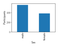
Figure S9: Demographic information about the participants of the experiment.

2 Experiment II

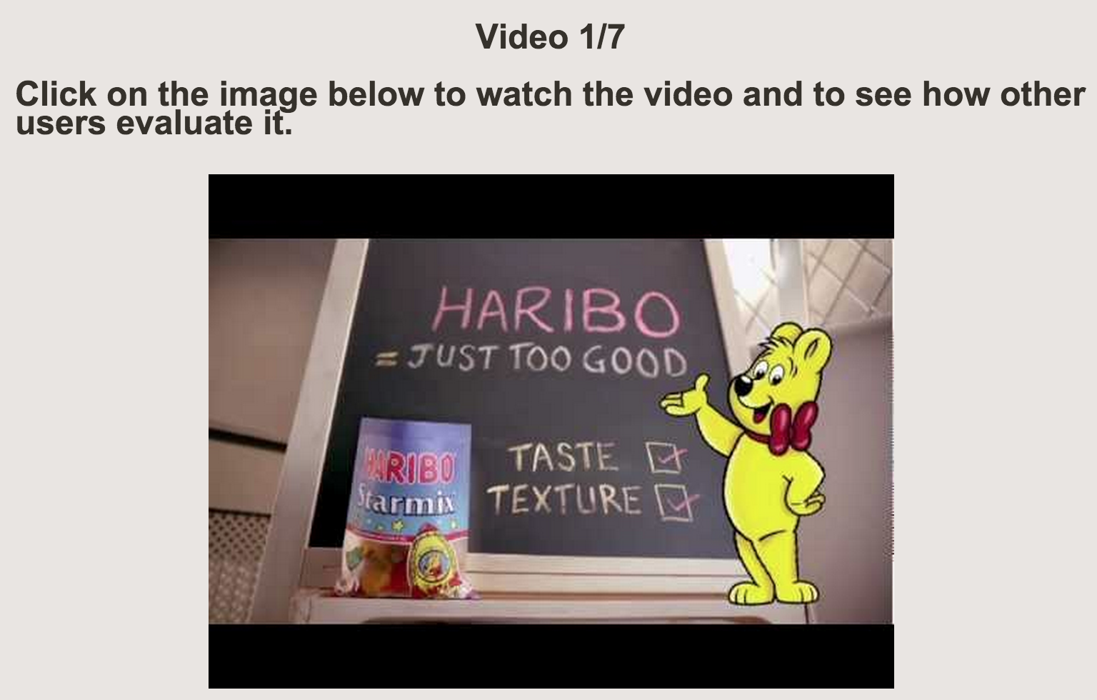
Figure S10: Participants access a video on YouTube or Vimeo by clicking on its thumbnail.

In this experiment, we track which exact comments are shown on the screens of the participant of the experiment and we use a sophisticated 200-point scale for measuring opinion. This experiment has two parts. Each of the parts is conducted with a different set of 7 videos on a different set of 700 participants. We split this experiment in two parts to avoid overloading the participants with evaluations of too many videos. In each part of this experiment, a participant is shown $7$ videos in a random order in $7$ different main experimental conditions assigned randomly to the videos.

2.1 Description

The participants are given the same instructions as in Experiment I. They are instructed to watch videos, to look at the feedback from other people about these videos, and to evaluate them. The subjects enter a webpage that looks like YouTube by clicking on a thumbnail of the video (Figure S10). For each video shown in the experiment, we ask the participant to evaluate whether she agrees or disagrees with the following statements (Figure S11). To measure the opinion, we ask about the agreement with the statement “I like this video”. The participant answer this statement using a slider bar in a scale from $100\%$ to $100\%$(Figure S12). We did not give the option of answering $0\%$ to avoid neutral answers. To measure the sharing willingness, we use the statement: “I’d share this video with friends” This statement can be answered with “Not Share/Share”. To test whether the participant agrees with other people’s feedback, we use the statement “I agree with the feedback of other people about this video (with the comments, thumbs)”. Additionally, we ask if the person have seen this video before, to account for the possibility of prior influence outside of the experiment. After having answered these questions for each of the videos, the participant is asked a short demographic survey (Figure S13).

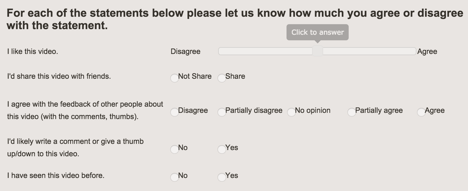
Figure S11: Questions asked for each video. The opinion is measured with the statement “I like this video”.

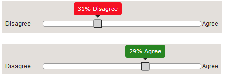
Figure S12: The psychometric scale for measuring opinion. The opinion is measured with the statement “I like this video”. Subjects answer this statement with a slider ranging from $100\%$ “Disagree” to $100\%$ “Agree”.

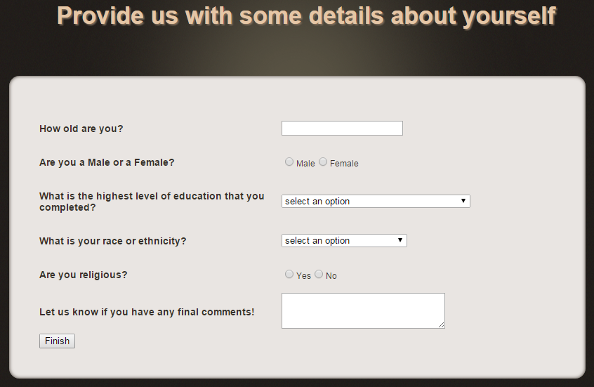
Figure S13: Demographic questions. After completing the survey for the seven videos the participant was asked to answer the following questions about personal demographic information.

2.2 Videos

For the experiments, we picked fourteen videos from YouTube of diverse quality, as judged by the fraction of thumbs up among thumbs (see Table S3). Note that in the main text, the fraction of thumbs up is used as an estimate of external opinion. We chose videos that have a public appeal but are not very popular, namely have from $100,000$ to $2$ million views, more than 50 comments, and over 100 thumbs (at the moment of data collection). Since we do not create any artificial comments and use only the original comments to manipulate the social feedback, we picked only videos that have both positive and negative comments. The links to the original videos and the numbers of each of the comment types, thumbs, and views for each of the videos are listed in Table S3. Average duration of the videos is $77$ seconds.

		Comments			Thumbs
Survey	Video	Pos.	Neut.	Neg.	Up	Down	Fraction up	Views	Link to the original
	ski lift	168	179	76	533	154	0.78	455,970	GP2wvGVCsIU
	ufo	55	136	317	140	1197	0.10	844,339	PCMklx9YvHQ
	shark prank	76	53	49	205	211	0.49	307,750	Rk1LXZgCSpE
Part I	fat talk	296	203	75	2796	79	0.97	154,843	V2SHwdtBH64
	pony shoes	196	217	653	439	1060	0.29	741,023	hJJtVUTWCcc
	rollers trick	24	41	35	638	164	0.80	254,765	qgSv8B6UiUY
	cat bath	148	156	105	1009	354	0.74	667,656	xR6j4ECkDT4
	feeding croc	48	16	34	576	58	0.91	836,942	EPW0m0mc6hc
	veet add	59	55	139	604	1377	0.30	661,311	UxCHLXQffsg
	google car	89	26	68	1713	23	0.99	123,721	aqrttLPjv1E
Part II	baby yoga	28	33	379	275	1996	0.12	870,166	fFwrZHFLe2E
	all nighter	288	582	232	12592	502	0.96	1,008,121	kFcnUsYKT5w
	skywalk	20	28	19	275	25	0.92	245,629	laveE4bUm3M
	haribo add	33	52	36	165	52	0.76	138,925	qc8vxx6J5Xw

Table S3: Basic statistics of the original, non-manipulated, videos: the number of comments of various types, the number of thumbs up and thumbs down, and the number of views at the time of their collection (February 2015).

2.3 Comments

Three labelers classified the comments as either positive, neutral, negative, or unreadable (see Table S3 for a summary). The Fleiss’ kappa between the three labelers is $0.56$. The comments that are unreadable or are written in a language different from English are filtered out. The ambivalent comments with conflicting labels, namely the comments that are labeled as both positive and negative by different labelers, are filtered out as well. In total, we filter out about $10\%$ of all comments. We apply a majority rule to determine the final label of each remaining comment.

During the experiment we measure which comments are shown to the participant on the screen. In order to see the comments, the participants need to scroll down, what allows precise measurements. Then, in the analysis, we estimate the number of comments read by the participant with the number of comments shown on the screen.

2.4 Data Processing

We apply the same filtering steps as for the data from Experiment I. As before, we discard the participants with incomplete answers, who gave answers more than once, or have answers invalidated for more than one videos (in total, less than $12\%$ of all participants).

Figure S14: The probability of positive opinion (left) and the sharing willingness (right) for the control condition (black circles) and the experimental conditions of various strength. The color of markers encodes positive (blue) and negative (red) conditions.

2.5 Demographics and Feedback of Participants

The participants of our experiments are slightly more likely to be male than female, predominantly white, young adults, with varying levels of education (see Figure S15). Many of them enjoyed participating in our experiments. Most of the voluntary comments left by the participants after the experiments express their positive sentiment and gratitude, e.g.: “I enjoyed this survey very much.”, “great videos! expected something boring”, and “fun videos. Thanks!”. Overall, $185$ participants voluntarily left positive feedback to our experiments containing at least one of these three words: “enjoy”, “great”, or “fun”.

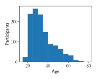
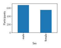
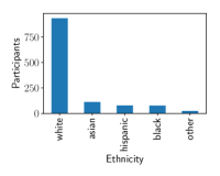
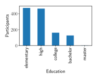
Figure S15: Demographic information about the participant of the experiment.

3 Models

3.1 Model Selection

Rank	Model	$-\log(P)$	#parameters	AIC
1	$P(\boldsymbol{\Delta n},\boldsymbol{y}|K=2,\underset{K\times V}{\boldsymbol{p}},\underset{1\times V}{\boldsymbol{a_{1}}},s_{1}\equiv 0,\underset{1\times V}{\boldsymbol{a_{2}}},s_{2})$	3316.4	43	6718.7
2	$P(\boldsymbol{\Delta n},\boldsymbol{y}|K=2,\underset{K\times V}{\boldsymbol{p}},a_{1},s_{1},\underset{1\times V}{\boldsymbol{a_{2}}},s_{2}\equiv 0)$	3330.7	30	6721.5
3	$P(\boldsymbol{\Delta n},\boldsymbol{y}|K=2,\underset{K\times 1}{\boldsymbol{p}},\underset{1\times V}{\boldsymbol{a_{1}}},s_{1}\equiv 0,\underset{1\times V}{\boldsymbol{a_{2}}},\underset{1\times V}{\boldsymbol{s_{2}}})$	3318.4	43	6722.8
4	$P(\boldsymbol{\Delta n},\boldsymbol{y}|K=2,\underset{K\times V}{\boldsymbol{p}},a_{1}\equiv 0,s_{1},\underset{1\times V}{\boldsymbol{a_{2}}},s_{2}\equiv 0)$	3332.4	29	6722.8
5	$P(\boldsymbol{\Delta n},\boldsymbol{y}|K=3,\underset{K\times V}{\boldsymbol{p}},a_{1},s_{1},a_{2},s_{2}\equiv 0,a_{3},s_{3}\equiv 0)$	3330.8	32	6725.5
6	$P(\boldsymbol{\Delta n},\boldsymbol{y}|K=2,\underset{K\times V}{\boldsymbol{p}},a_{1},\underset{1\times V}{\boldsymbol{s_{1}}},\underset{1\times V}{\boldsymbol{a_{2}}},s_{2}\equiv 0)$	3320.1	43	6726.2
7	$P(\boldsymbol{\Delta n},\boldsymbol{y}|K=3,\underset{K\times V}{\boldsymbol{p}},a_{1},s_{1}\equiv 0,a_{2},s_{2}\equiv 0,a_{3}\equiv 0,s_{3})$	3332.4	31	6726.8
8	$P(\boldsymbol{\Delta n},\boldsymbol{y}|K=3,\underset{K\times 1}{\boldsymbol{p}},\underset{1\times V}{\boldsymbol{a_{1}}},\underset{1\times V}{\boldsymbol{s_{1}}},\underset{1\times V}{\boldsymbol{a_{2}}},s_{2}\equiv 0,a_{3}\equiv 0,\underset{1\times V}{\boldsymbol{s_{3}}})$	3307.5	58	6730.9
9	$P(\boldsymbol{\Delta n},\boldsymbol{y}|K=3,\underset{K\times 1}{\boldsymbol{p}},\underset{1\times V}{\boldsymbol{a_{1}}},\underset{1\times V}{\boldsymbol{s_{1}}},\underset{1\times V}{\boldsymbol{a_{2}}},s_{2}\equiv 0,a_{3}\equiv 0,s_{3}\equiv 0)$	3322.9	44	6733.8
10	$P(\boldsymbol{\Delta n},\boldsymbol{y}|K=2,\underset{K\times V}{\boldsymbol{p}},a_{1}\equiv 0,\underset{1\times V}{\boldsymbol{s_{1}}},\underset{1\times V}{\boldsymbol{a_{2}}},s_{2}\equiv 0)$	3325.0	42	6733.9

Table S4: The list of top variants of the sub-population model. The variants are ranked by the value of AIC. All top variants have $s_{k}\equiv 0$ for at least one sub-population.

Survey	Video	$p_{2}$	$\sigma(p_{2})$			$a_{2}$	$\sigma(a_{2})$			$a_{1}$	$\sigma(a_{1})$
	ski lift	0.32	0.01	0.05	0.06	3.44	2.29	5.90	1.28	-0.75	0.02	0.23	0.20
	ufo	0.11	0.02	0.06	0.04	-1.87	3.35	5.37	2.43	-3.84	0.08	0.40	0.38
	shark prank	0.16	0.01	0.05	0.05	1.77	0.60	5.01	1.70	-1.47	0.02	0.19	0.21
Part I	fat talk	0.17	0.01	0.07	0.06	-8.28	3.19	8.95	2.00	0.80	0.07	0.30	0.19
	pony shoes	0.12	0.00	0.10	0.07	-9.67	4.07	7.01	3.99	-2.37	0.02	0.22	0.21
	rollers trick	0.40	0.01	0.04	0.05	-0.22	0.13	1.16	0.74	-0.25	0.01	0.17	0.17
	cat bath	0.35	0.01	0.05	0.05	1.39	0.36	2.89	0.86	0.17	0.01	0.17	0.17
	feeding croc	0.29	0.07	0.16	0.06	15.51	1.58	3.74	1.28	0.59	0.16	0.43	0.20
	veet add	0.15	0.03	0.12	0.04	3.04	0.65	2.32	2.43	-0.15	0.03	0.68	0.38
	google car	0.05	0.01	0.13	0.05	1.59	1.59	3.64	1.70	2.43	0.05	0.39	0.21
Part II	baby yoga	0.20	0.05	0.16	0.06	0.50	0.81	2.00	2.00	-2.52	0.08	0.42	0.19
	all nighter	0.15	0.03	0.10	0.07	-3.60	1.68	1.96	3.99	1.06	0.07	0.63	0.21
	skywalk	0.18	0.05	0.18	0.05	1.47	0.31	1.99	0.74	1.89	0.05	1.07	0.17
	haribo add	0.21	0.04	0.12	0.05	-0.93	0.47	1.55	0.86	0.89	0.04	0.31	0.17

Table S5: The values of parameters of the best sub-population model and their standard error. The standard error is estimated using three methods, from left to right: jackknife re-sampling, bootstrap re-sampling, and observed Fisher information. Note that the standard error of prior opinions of influenceable sub-population is many times larger, i.e., $\sigma(a_{2})>\sigma(a_{1})$.

The model of sub-populations does not determine what is the best number of sub-populations nor whether all parameters $p_{kv}$, $a_{kv}$, and $s_{kv}$ are indeed necessary. Each of these parameters can depend on the video, can be shared across the videos, e.g., $p_{kv}\equiv p_{k}$, or vanish by being replaced with a fixed neutral value across videos, i.e., $p_{kv}\equiv 1/K$, or $\displaystyle\mathop{\forall}_{v}a_{kv}=0$, or $\displaystyle\mathop{\forall}_{v}s_{kv}=0$. We represent the structure of the model using the aforementioned notation for the likelihood,

$$P(\boldsymbol{\Delta n},\boldsymbol{y}|k,\underset{K\times V}{\boldsymbol{p}},\underset{1\times V}{\boldsymbol{a_{1}}},\underset{1\times V}{\boldsymbol{s_{1}}},\dots,\underset{1\times V}{\boldsymbol{a_{K}}},\underset{1\times V}{\boldsymbol{s_{K}}}),$$ (13)

which states that the parameters $p$, $a_{1}$, $s_{1}$, $\dots$, $a_{K}$, $s_{K}$ depend on the videos. As an example, we show the representation of the model with $K=2$ sub-populations, vanishing $s_{1}$, parameter $s_{2}$ independent from videos, and the remaining parameters dependent on videos:

$$P(\boldsymbol{\Delta n},\boldsymbol{y}|K=2,\underset{K\times V}{\boldsymbol{p}},\underset{1\times V}{\boldsymbol{a_{1}}},s_{1}\equiv 0,\underset{1\times V}{\boldsymbol{a_{2}}},s_{2}),$$ (14)

which is the variant introduced in the main text of this manuscript that maximizes Akaike information criterion (AIC). In other words, each of the parameters of a model variant takes one of $N=3$ different forms and each sub-population is defined by one of $N^{2}$ combinations of parameters. The sub-populations are interchangeable, so in total there is $N\times\left[\binom{N^{2}+K-1}{K}\right]$ variants of the model for $K$ sub-populations. Note, however, that a model with more than one sub-population with vanishing parameters, i.e., multiple sub-populations $k$ such that $\displaystyle\mathop{\forall}_{v}a_{kv}=0$ and $\displaystyle\mathop{\forall}_{v}s_{kv}=0$, is equivalent to a model having just one such sub-population. Hence, overall, for $K$ sub-populations there are $N\times\left[\binom{N^{2}+K-1}{K}-\binom{N^{2}+K-3}{K-2}\right]$ different variants of the sub-populations model.

We fit each variant of sub-populations model for $K\in\{1,2,\dots,6\}$ by maximizing the log-likelihood of the corresponding model (Equation 10). To this end, we perform $1000$ realizations of the L-BFGS-B algorithm, each time initializing the parameters with random values sampled from a standard normal distribution, with the exception of $p_{kv}$, which is always initialized with the uniform distribution of individuals over sub-populations, i.e., $p_{kv}=1/K$. Different variants of sub-populations model generally have varying number of parameters and sub-populations. After fitting these variants of the model, we compare them using AIC, which penalizes for the number of parameters. We plot the best values of AIC and log-likelihood against the number of parameters and sub-populations (Figure S16). The models achieving low AIC tend to have two sub-populations and less than $50$ parameters, that is about $3$ parameters per video. The top ten best variants of the models are shown in Table S4. Out of these ten models, six have two sub-populations, while four have three sub-populations. In all cases, among these sub-populations, there is at least one non-influenceable sub-population ($\displaystyle\mathop{\forall}_{v}s_{kv}=0$). The four top variants of the sub-population model are very similar to the top model presented in the main text, while the remaining top models are also similar, but may have an additional sub-population. Overall, the findings shown in the main text for the top model are consistent with the other top ten models.

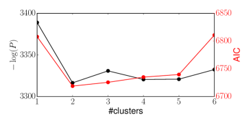
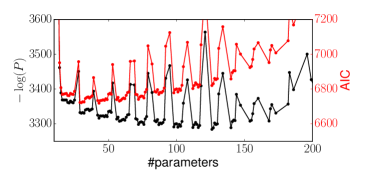
Figure S16: The minimal negative log-likelihood and Akaike information criterion of the sub-population model having a given number of clusters (top) or parameters (bottom).

3.2 Parameters of the Best Model

The best sub-population model is $P(\boldsymbol{\Delta n},\boldsymbol{y}|K=2,\underset{K\times V}{\boldsymbol{p}},\underset{1\times V}{\boldsymbol{a_{1}}},s_{1}\equiv 0,\underset{1\times V}{\boldsymbol{a_{2}}},s_{2})$. It has two sub-populations: non-influenceable sub-population with influenceability $s_{1}\equiv 0$ and influenceable sub-population having $s_{2}=0.8\pm 0.005$. We list the value of the remaining parameters for each video in Table S5. Individuals in influenceable sub-population have much noisier prior opinions about each video than individuals in non-influenceable sub-populations (Figure S17).

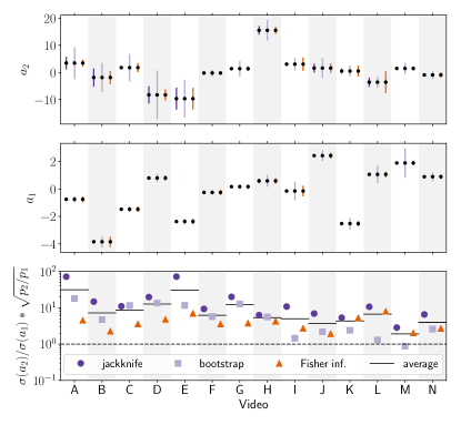
Figure S17: The values of parameters with their standard errors of the best sub-population model for influenceable (top) and non-influenceable (middle) sub-population. The standard deviation is computed using three different methods, from left to right: jackknife re-sampling, bootstrap re-sampling, and the inverse of observed Fisher information. The bottom figure shows the ratio of sub-populations’ standard-deviation corrected for their sizes.

References

- (1) Lippmann W (1922) Public opinion. (Harcourt, Brace and Company, New York).
- (2) Herman ES, Chomsky N (1988) Manufacturing Consent: The Political Economy of the Mass Media. (Pantheon Books, New York).
- (3) Richtel M (2013) There’s Power in All Those User Reviews. New York Times.
- (4) King G, Pan J, Roberts ME (2016) How the Chinese Government Fabricates Social Media Posts for Strategic Distraction, not Engaged Argument. American Political Science Review 111(917):484–501.
- (5) Cho CH, Martens ML, Kim H, Rodrigue M (2011) Astroturfing Global Warming: It Isn’t Always Greener on the Other Side of the Fence. Journal of Business Ethics 104(4):571–587.
- (6) Lazer DMJ, et al. (2018) The science of fake news. Science 359(6380):1094–1096.
- (7) Vosoughi S, Roy D, Aral S (2018) The spread of true and false news online. Science 359(6380):1146–1151.
- (8) Asch SE (1955) Opinions and Social Pressure. Scientific American 193(5):31–35.
- (9) Sherif M (1935) A study of some social factors in perception. Archives of Psychology (Columbia University) 187:60.
- (10) Eguíluz VM, Masuda N, Fernández-Gracia J (2015) Bayesian Decision Making in Human Collectives with Binary Choices. PLOS ONE 10(4):e0121332.
- (11) Muchnik L, Aral S, Taylor SJ (2013) Social influence bias: a randomized experiment. Science (New York, N.Y.) 341(6146):647–51.
- (12) Wang T, Wang D, Wang F (2014) Quantifying herding effects in crowd wisdom in Proceedings of the 20th ACM SIGKDD international conference on Knowledge discovery and data mining - KDD ’14. pp. 1087–1096.
- (13) Sipos R, Ghosh A, Joachims T (2014) Was This Review Helpful to You?: It Depends! Context and Voting Patterns in Online Content in Proceedings of the 23rd International Conference on World Wide Web, WWW ’14. (ACM, New York, NY, USA), pp. 337–348.
- (14) Kramer ADI, Guillory JE, Hancock JT (2014) Experimental evidence of massive-scale emotional contagion through social networks. Proceedings of the National Academy of Sciences 111(24):8788–8790.
- (15) Kelman HC (1961) Processes of Opinion Change. Public Opinion Quarterly 25(1):57–78.
- (16) Wood W (2000) Attitude Change: Persuasion and Social Influence. Annual Review of Psychology 51(1):539–570.
- (17) Cialdini RB, Goldstein NJ (2004) Social influence: compliance and conformity. Annual Review of Sociology 55(1974):591–621.
- (18) Turner JC, Hogg MA, Oakes PJ, Reicher SD, Wetherell MS (1987) Rediscovering the social group: A self-categorization theory. (Basil Blackwell, Cambridge, MA, US).
- (19) Phillips L, Edwards W (1966) Conservatism in a simple propabilistic inference task. Journal of Experimental Psychology 72(3):346–354.
- (20) Tversky A, Kahneman D (1974) Judgment under Uncertainty: Heuristics and Biases. Science 185(4157):1124–1131.
- (21) Navajas J, et al. (2017) The idiosyncratic nature of confidence. Nature Human Behaviour 1(11):810–818.
- (22) Benjamin DJ (2019) Errors in probabilistic reasoning and judgment biases in Handbook of Behavioral Economics - Foundations and Applications 2, eds. Bernheim BD, Dellavigna S, Laibson D.
- (23) Edwards W, Lindman H, Savage LJ (1963) Bayesian statistical inference for psychological research. Psychological Review 70(3):193–242.
- (24) Grether DM (1980) Bayes Rule as a Descriptive Model: The Representativeness Heuristic. The Quarterly Journal of Economics 95(3):537.
- (25) Buhrmester M, Kwang T, Gosling SD (2011) Amazon’s Mechanical Turk: A New Source of Inexpensive, Yet High-Quality, Data? Perspectives on Psychological Science 6(1):3–5.
- (26) Heider F (1958) The Psychology of Interpersonal Relations. (New York: Wiley).
- (27) Pérez-Escudero A, de Polavieja GG (2011) Collective Animal Behavior from Bayesian Estimation and Probability Matching. PLoS Computational Biology 7(11):e1002282.
- (28) Arganda S, Pérez-Escudero A, de Polavieja GG (2012) A common rule for decision making in animal collectives across species. Proceedings of the National Academy of Sciences of the United States of America 109(50):20508–13.
- (29) Bikhchandani S, Hirshleifer D, Welch I (1992) A Theory of Fads, Fashion, Custom, and Cultural Change as Informational Cascades. Journal of Political Economy 100(5):992–1026.
- (30) Easley D, Kleinberg J (2012) Networks, Crowds, and Markets: Reasoning about a highly connected world. (Cambridge University Press).
- (31) Madirolas G, de Polavieja GG (2015) Improving Collective Estimations Using Resistance to Social Influence. PLOS Computational Biology 11(11):e1004594.
- (32) Stone M (1977) An Asymptotic Equivalence of Choice of Model by Cross-Validation and Akaike’s Criterion. Journal of the Royal Statistical Society: Series B (Statistical Methodology) 39(1):44–47.
- (33) Krafft PM, et al. (2016) Human collective intelligence as distributed Bayesian inference.
- (34) Tenenbaum JB, Kemp C, Griffiths TL, Goodman ND (2011) How to grow a mind: statistics, structure, and abstraction. Science (New York, N.Y.) 331(6022):1279–1285.
- (35) Campolo A, Sanfilippo M, Whittaker M, Crawford K (2018) AI Now 2017 Report. (AI Now Institute at New York University).
- (36) Treiblmaier H, Filzmoser P (2011) Benefits from Using Continuous Rating Scales in Online Survey Research in International Conference on Information Systems (ICIS).
- (37) Behrend ER, Bitterman ME (1961) Probability-Matching in the Fish. The American Journal of Psychology 74(4):542–551.
- (38) Kirk KL, Bitterman ME (1965) Probability-Learning by the Turtle. Science (New York, N.Y.) 148(3676):1484–1485.
- (39) Wozny DR, Beierholm UR, Shams L (2010) Probability Matching as a Computational Strategy Used in Perception. PLoS Computational Biology 6(8):e1000871.
- (40) Eggenberger F, Pólya G (1923) Über die Statistik verketteter Vorgänge. ZAMM - Journal of Applied Mathematics and Mechanics / Zeitschrift für Angewandte Mathematik und Mechanik 3(4):279–289.
- (41) Mahmoud H (2008) Polya Urn Models. (CRC Press).
- (42) Alajaji F, Fuja T (1994) A communication channel modeled on contagion - Information Theory, IEEE Transactions on. 40(6):2035–2041.
- (43) Hayhoe M, Alajaji F, Gharesifard B (2018) A Polya Contagion Model for Networks. IEEE Transactions on Control of Network Systems 5(4):1998–2010.
- (44) Sedghi H, Janzamin M, Anandkumar A (2016) Provable Tensor Methods for Learning Mixtures of Generalized Linear Models in Proceedings of the 19th International Conference on Artificial Intelligence and Statistics, Proceedings of Machine Learning Research, eds. Gretton A, Robert CC. (PMLR, Cadiz, Spain), Vol. 51, pp. 1223–1231.