Non-equilibrium and non-homogeneous phenomena around a first-order quantum phase transition

Abstract

We consider non-equilibrium phenomena in a very simple model that displays a zero-temperature first-order phase transition. The quantum Ising model with a four-spin exchange is adopted as a general representative of first-order quantum phase transitions that belong to the Ising universality class, such as for instance the order-disorder ferroelectric transitions, and possibly first-order $T=0$ Mott transitions. In particular, we address quantum quenches in the exactly solvable limit of infinite connectivity and show that, within the coexistence region around the transition, the system can remain trapped in a metastable phase, as long as it is spatially homogeneous so that nucleation can be ignored. Motivated by the physics of nucleation, we then study in the same model static but inhomogeneous phenomena that take place at surfaces and interfaces. The first order nature implies that both phases remain locally stable across the transition, and with that the possibility of a metastable wetting layer showing up at the surface of the stable phase, even at $T$=0. We use mean-field theory plus quantum fluctuations in the harmonic approximation to study quantum surface wetting.

I Introduction

The last few years have witnessed a growing interest in the non-equilibrium dynamics of systems driven across quantum phase transitionsBarmettler et al. (2010); Eckstein et al. (2009a); Polkovnikov et al. (2011), largely but not exclusively stimulated by experiments on ultracold atomsBloch et al. (2008). A rich theoretical activity thus focused on such systems, for example on the superfluid to Mott insulator transition in the one-dimensional Bose-Hubbard modelGreiner et al. (2002); Kollath et al. (2007); Bakr et al. (2010); Carleo et al. (2012) or on the ferromagnetic to paramagnetic transition in the quantum Ising chainMeinert et al. (2013); Rossini et al. (2009); Calabrese et al. (2011). In addition, studies have dealt with quantum phase transitions in solid state systems, experimentally accessed by time-resolved pump-probe spectroscopies. That is for instance the case of the metal-insulator Mott transition in the Fermi-Hubbard modelEckstein et al. (2009b); Schiró and Fabrizio (2010). This is a prototypical model of strongly-correlated materials, whose rich phase diagram offers an ideal playground for out-of-equilibrium continuous phase transitions Cavalleri et al. (2001); Kübler et al. (2007); Takubo et al. (2008); Beaud et al. (2009); Petersen et al. (2011); Ichikawa et al. (2011); Ehrke et al. (2011); Liu et al. (2012); Stojchevska et al. (2014); Wegkamp et al. (2014).

However, phase transitions in real materials, including quantum ones, are far more commonly discontinuous, while most of theoretical analyses focused so far on continuous quantum phase transitions. It is therefore important to identify and describe what novel features are brought about by the first order character and how they might show up in experiments.

Here we take a first step in this direction by studying a very simple infinitely-connected model that displays a zero-temperature first-order transition. The simplicity of the model allows for exact results even in out-of-equilibrium conditions and may serve both as a reference example as well as a starting point for the successive addition of quantum fluctuations, which we shall partly undertake when dealing with interface wetting.

I.1 Outline and summary of the main results

The paper is divided into two parts. In the first, which comprises sections II and III, we study the out of equilibrium dynamics of an exactly solvable infinitely connected quantum Ising model with a quartic spin-spin exchange. This model, as function of the transverse field $h$, displays a zero-temperature discontinuous transition from an ordered phase at $h<h_{c}$, where $Z_{2}$ symmetry is spontaneously broken, to a disordered one at $h>h_{c}$. A first-order quantum Ising phase transition should be relevant for the order-disorder para- to ferro-electric transition, but we speculate it might be representative also of discontinuous Mott transitions, as discussed in section II.2. Because of the first order character, around $h_{c}$ there is coexistence between the two different phases, one being stable and the other metastable. The non-equilibrium protocol that we implement consists in a sudden quench of the transverse field, $h=h_{i}\to h_{f}$, starting from the ordered phase, i.e. with the initial $h_{i}<h_{c}$. We show that, because of coexistence, the system can remain trapped into an ordered state even though $h_{f}>h_{c}$. In this very peculiar solvable limit such result arises from a nice property of the microcanonical ensemble accessible by the unitary time-evolution. Indeed, in a certain range of transverse fields around $h_{c}$, the many-body spectrum includes a region of (extensive) eigenvalues where symmetry variant and invariant eigenstates coexist. Therefore, even though the low energy eigenvalues are symmetry invariant, i.e. the ground state is disordered, if the initial wavefunction has a finite overlap with the symmetry variant eigenstates the unitary evolution does not restore the $Z_{2}$ symmetry. In section III.1 we further exploit this property showing that an external stimulus that acts for a finite time can drive the stable phase into the metastable one.

A finite-temperature first-order phase transition can still show criticality due to wetting at an interface, a phenomenon that has been extensively studied since more than thirty years Cahn (1977); Lipowsky (1982). Not much it is known about wetting when the first order transition occurs instead at zero temperature. One can invoke the quantum-classical mapping and reasonably guess that the critical properties at zero temperature in $d$ dimensions should correspond to those of classical wetting in $d+1$ dimensions, actually $d+z$ where $z$ is the dynamical critical exponent. Hertz (1976) However, we think it is still worth uncovering what exactly wetting means in a quantum model that undergoes a first order transition as function of a Hamiltonian parameter, which is the content of the second part of this paper, section IV. We first study wetting in the simplest extension of the infinitely connected quantum Ising model that consists of a slab where the spins are infinitely connected within each layer, which is however only coupled to its nearest neighbours. This model thus effectively maps onto a one-dimensional spin system, where each spin represents the total spin of each individual layer, hence it is of the order of its number of sites. A semiclassical analysis of this model, which corresponds to the conventional spin-wave approximation, as shown in the Appendix and justified by the fact that the spin magnitude is large, shows that the gapped spin-wave excitation spectrum develops a bound state localised just at the wetting interface. We find that this bound state is unique and its energy vanishes at the first order transition. Because of the infinite connectivity we find, not surprisingly, that the critical properties of the saddle point are mean-field like and correspond to classical wetting in high dimensions. However the singular behaviour of quantum fluctuations is different from that of classical fluctuations at finite temperature.
In section IV.5 we briefly discuss by means of spin-wave theory what should change in a more realistic three dimensional system where each layer is not infinitely stiff because of a finite connectivity. In this case the bound state develops into a branch of excitations that are still localised around the position of the wetting interface but disperse in the perpendicular direction. This surface, or, better, capillary wave is coherent, being below the continuum of bulk excitations, and goes soft at the first order transition. However such softening does not produce the logarithmic singularities that in the classical case signal interface roughening because of the extra dimension brought by quantum mechanics.
The final section V is devoted to concluding remarks, especially concerning our speculated relationship between a first-order zero-temperature Ising transition and first-order Mott transitions.

II The model

Spin models on completely connected graphs have been largely studied in the context of continuous quantum phase transitionsBapst and Semerjian (2012); Sciolla and Biroli (2010, 2011); Sandri et al. (2012); Mazza and Fabrizio (2012), providing results that are quite instructive. Our goal now is to move on to first order quantum phase transitions.

We consider the quantum Ising model of spins 1/2 on an $N$-site lattice

$$\mathcal{H} = -\sum_{i,j}\,J^{(2)}_{ij}\;\sigma^{z}_{i}\,\sigma^{z}_{j}-h\,\sum_{i}\,\sigma^{x}_{i}$$ (1)

$$\qquad-\sum_{i,j,k,l}\,J^{(4)}_{ijkl}\;\sigma^{z}_{i}\,\sigma^{z}_{j}\,\sigma^{z}_{k}\,\sigma^{z}_{l}$$

$$= \bigg{(}-\frac{1}{N}\,J^{(2)}\,\big{(}\sigma^{z}_{\mathbf{0}}\big{)}^{2}\,-h\,\sigma^{x}_{\mathbf{0}}-\frac{1}{N^{3}}\,J^{(4)}\,\big{(}\sigma^{z}_{\mathbf{0}}\big{)}^{4}\bigg{)}$$

$$+\bigg{(}-\frac{1}{N}\,\sum_{\mathbf{q}\not=\mathbf{0}}\,J^{(2)}_{\mathbf{q}}\;\sigma^{z}_{\mathbf{q}}\,\sigma^{z}_{-\mathbf{q}}$$

$$-\frac{1}{N^{3}}\,\sum_{(\mathbf{k}\mathbf{p}\mathbf{q})\not=(\mathbf{0}\mathbf{0}\mathbf{0})}\,J^{(4)}_{\mathbf{k}\mathbf{p},\mathbf{q}}\,\sigma^{z}_{\mathbf{k}}\,\sigma^{z}_{\mathbf{p}+\mathbf{q}}\,\sigma^{z}_{-\mathbf{p}}\,\sigma^{z}_{-\mathbf{k}-\mathbf{q}}\bigg{)}$$

$$= \mathcal{H}_{\mathbf{0}}+\delta\mathcal{H},$$

where $\sigma^{a}_{i}$, $a=x,y,z$, are Pauli matrices, $J^{(2)}=J^{(2)}_{\mathbf{0}}$ and $J^{(4)}=J^{(4)}_{\mathbf{0}\mathbf{0},\mathbf{0}}$ are the Fourier transforms of the two-spin and four-spin exchange constants at zero momentum. The multi-spin exchange is known to lead to first order transitions. For instance, the Ising model with four spin interaction has been invoked to describe the first order paraelectric-ferroelectric phase transition, especially in order-disorder ferroelectrics. Wang et al. (1989) In Eq. (1), $\mathcal{H}_{\mathbf{0}}$ includes only Fourier components at $\mathbf{q}=\mathbf{0}$, while $\delta\mathcal{H}$ embodies all remaining terms. In the limit of long-range exchange we can discard $\delta\mathcal{H}$ and just study the mean-field Hamiltonian $\mathcal{H}_{\mathbf{0}}$. Successively, we could treat $\delta\mathcal{H}$ perturbatively, for instance in the spin-wave approximationSandri et al. (2012), which would amount to add spatial quantum fluctuations to the mean-field results.

The Hamiltonian $\mathcal{H}_{\mathbf{0}}$, which corresponds to an infinitely connected Lipkin-Ising model, was studied in non-equilibrium conditions by Bapst and Semerjian in Ref. Bapst and Semerjian, 2012, see also Ref. Sciolla and Biroli, 2011. Here we shall closely follow their work and extend it to account for a larger variety of out-of-equilibrium situations.

II.1 Equilibrium properties of $\mathcal{H}_{\mathbf{0}}$

We start from the equilibrium phase diagram of $\mathcal{H}_{\mathbf{0}}$. We set $J^{(4)}$ as our energy unit, and define $\gamma=J^{(2)}/J^{(4)}$ and $h/J^{(4)}\to h$.

Observing that $\mathcal{H}_{\mathbf{0}}$ commutes with the total spin

$$\mathbf{S}^{2}=\bigg{(}\frac{1}{2}\,\sum_{i}\,\boldsymbol{\sigma}_{i}\bigg{)}^{2}=S(S+1),$$ (2)

the Hilbert space decomposes into subspaces with fixed total spin $S=0,1,\dots,M$, assuming $N=2M$ an even integer. Each subspace comprises eigenstates of the Hamiltonian

$$\mathcal{H}_{\mathbf{0}}(S)=-\frac{4}{N}\,\gamma\,\Big{(}S^{z}\Big{)}^{2}-\frac{16}{N^{3}}\,\Big{(}S^{z}\Big{)}^{4}-2h\,S^{x},$$ (3)

each with degeneracy

$$g(S)=\binom{2M}{M+S}-\binom{2M}{M+S+1},$$ (4)

which is the number of ways to couple $N$ 1/2 spins into total spin $S$. If we define $S=M\,s$, then, in the thermodynamic limit $M\to\infty$, $s$ effectively becomes a continuous variable, $s\in[0,1]$, and the partition function can be evaluated semiclassicallyLieb (1973)

$$Z = \sum_{S}\,g(S)\,\sum_{S^{z}=-S}^{S}\,\langle S,S^{z}\mid\text{e}^{-\beta\,\mathcal{H}_{\mathbf{0}}(S)}\mid S,S^{z}\rangle$$

$$\simeq \int_{0}^{1}\!\!\!ds\,\frac{\displaystyle M\big{(}2Ms+1\big{)}}{\displaystyle 4\pi}\int\!d\!\cos\theta\,d\phi\;\text{e}^{-N\beta\,F(\theta,\phi,s)},$$

where the semiclassical free-energy density reads

$$F(\theta,\phi,s) = -\gamma\,s^{2}\!\cos^{2}\theta-s^{4}\!\cos^{4}\theta$$ (6)

$$\!\!-h\,s\sin\theta\,\cos\phi-T\,\mathcal{S}(s),$$

with entropy

$$\mathcal{S}(s) = \frac{1}{2M}\,\ln g\big{(}Ms)\big{)}\simeq-\frac{\displaystyle 1+s}{\displaystyle 2}\,\ln\frac{\displaystyle 1+s}{\displaystyle 2}$$ (7)

$$-\frac{\displaystyle 1-s}{\displaystyle 2}\,\ln\frac{\displaystyle 1-s}{\displaystyle 2}+O\big{(}M^{-1}\big{)}.$$

For $M\to\infty$ we can approximate the integral by its saddle point value, which corresponds to $\cos\phi=1$ and, upon defining $m=\cos\theta\in[-1,1]$, to the minimum of

$$F(m,s) = -\gamma\,s^{2}m^{2}-s^{4}m^{4}-hs\,\sqrt{1-m^{2}}-T\,\mathcal{S}(s)$$ (8)

$$= E(m,s)-T\,\mathcal{S}(s),$$

with respect to both $s$ and $m$.

At fixed $s$, the extrema of $E(m,s)$ satisfy

$$m\bigg{[}h-\sqrt{1-m^{2}}\;\Big{(}2\gamma s+4s^{3}m^{2}\Big{)}\bigg{]}=0,$$ (9)

so that $m=0$ is always an extremum, actually a maximum whenever $4\gamma^{2}s^{2}>h^{2}$. We define $t\equiv\sqrt{1-m^{2}}\in[0,1]$ so that, apart from $m=0$, the other extrema satisfy the cubic equation

$$t^{3}-\Big{(}1+\frac{\gamma}{2s^{2}}\Big{)}\,t+\frac{\displaystyle h}{\displaystyle 4s^{3}}\equiv t^{3}-a\,t+b=0,$$ (10)

whose roots are acceptable solutions only if real, positive and smaller than one. Solving Eq. (10), we find three distinct regimes:

• If

  $$h^{2}\geq\frac{8}{27}\,\big{(}2s^{2}+\gamma\big{)}^{3},$$ (11)

  or

  $$\Big{(}4\gamma^{2}s^{2}\leq h^{2}\leq\frac{8}{27}\,\big{(}2s^{2}+\gamma\big{)}^{3}\Big{)}\,\land\,\Big{(}\gamma\geq 4s^{2}\Big{)},$$ (12)

  there is only one minimum at $m=0$.

• If

  $$h^{2}\leq 4\gamma^{2}s^{2},$$ (13)

  then $m=0$ is a maximum and there are two equivalent minima at

  $$m_{\pm}=\pm m_{*}=\pm\sqrt{1-t_{*}^{2}},$$ (14)

  where

  $$t_{*}=2\sqrt{\frac{\displaystyle a}{\displaystyle 3}}\;\cos\zeta,$$ (15)

  with

  $$\zeta=\frac{\displaystyle 2\pi}{\displaystyle 3}-\frac{1}{3}\,\mbox{tan}^{-1}\frac{\displaystyle\sqrt{\frac{\displaystyle 4a^{3}}{\displaystyle 27}-b^{2}}}{\displaystyle b}\in\Big{[}\frac{\pi}{3},\frac{\pi}{2}\Big{]}.$$ (16)

  Because of the finite magnetisation $m_{*}$, the $Z_{2}$ symmetry is spontaneously broken.

• Finally, when

  $$\Big{(}4\gamma^{2}s^{2}\leq h^{2}\leq\frac{8}{27}\,\big{(}2s^{2}+\gamma\big{)}^{3}\Big{)}\,\land\,\Big{(}\gamma\leq 4s^{2}\Big{)},$$ (17)

  there are three minima, one at $m=0$ and the two equivalent symmetry-breaking minima Eq. (14), with the same $t_{*}$ as in Eq. (15). The absolute minimum depends on the value of $E(0,s)$ with respect to $E\big{(}\pm m_{*},s\big{)}$.

It follows that each individual subspace at fixed $s$ undergoes a quantum phase transition from an ordered ground state with finite magnetisation below a critical $h_{*}(s)$ to a disordered one above. The critical $h_{*}(s)$ is lower the lower $s$; the transition is first order if $\gamma\leq 4s^{2}$ and second order otherwise. Conversely, at fixed $h$, there exists a critical $s_{*}(h)$ such that the ground states of all subspaces with $s\geq s_{*}(h)$ are ordered while those of the subspaces with $s<s_{*}(h)$ are disordered.

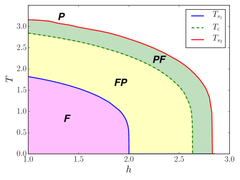
Figure 1: (Color online) Phase diagram of the model $\mathcal{H}_{0}$, Eq. (1), at $\gamma=1$. In the region labelled as F there is only a ferromagnetic free-energy minimum, i.e. the $Z_{2}$ symmetry is broken. Conversely, in the region P there is only a paramagnetic minimum. The coexistence regions are FP and PF, where in FP the absolute minimum is ferromagnetic, while in PF is paramagnetic. The F-P phase transition occurs where the free energies cross along the dotted line $T_{c}$ separating FP from PF. The solid lines $T_{s_{1}}$ between F and FP, and $T_{s_{2}}$ between P and PF, are spinodal lines where an additional metastable free energy minimum, P and F, respectively, appears besides the stable one, F and P respectively.

Let us analyse the above results more in detail. At $T=0$, the ground state is in the $s=1$ subspace. We shall always assume that

$$\gamma<4,$$ (18)

so that, with $s=1$, the only possibilities are Eqs. (11), (13) and (17). It thus follows that at $h^{2}\leq 4\gamma^{2}$, the symmetry is broken and $m=\pm m_{*}$. In the region

$$4\gamma^{2}\leq h^{2}\leq\frac{8}{27}\,\big{(}2+\gamma\big{)}^{3},$$ (19)

there is coexistence between a symmetry broken solution, $m=\pm m_{*}$, and a symmetry invariant one, $m=0$. The two solutions cross at a critical $h_{c}=h_{*}(s=1)$, which signals a first order quantum phase transition. Finally, for

$$h^{2}\geq\frac{8}{27}\,\big{(}2+\gamma\big{)}^{3},$$ (20)

the symmetry broken solution is no longer stable.

Suppose now that $h<h_{c}$, so that at $T=0$ the $Z_{2}$ symmetry is spontaneously broken. At finite temperature, $T\not=0$, because of the entropy term Eq. (7), the free energy minimum is obtained, see Eq. (8), for a value of the total spin $s=s(T)<1$, which diminishes with increasing $T$. Therefore, there exists a critical temperature $T_{c}$ at which $s\big{(}T_{c}\big{)}\leq s_{*}(h)$, where the symmetry is recovered. Specifically, if we assume Eq. (18), the transition remains first order at any finite $T$. The phase diagram at $\gamma=1$ is shown in Fig. 1 for $h\geq 1$.

Figure 2: (Color online) The function $f_{+}(m)$ and $f_{-}(m)$ for $s=1$, $\gamma=1$ and $h=1.9$, which correspond to the case in which the ground state breaks spontaneously $Z_{2}$. The regions above $f_{+}(m)$ and below $f_{-}(m)$ are unaccessible when $N\to\infty$. Also shown is the energy threshold $\epsilon_{*}$ above which symmetry is restored.

II.2 Links to the Mott transition

As was said above, the Ising model with a four spin exchange, Eq. (1), describes the first order paraelectric-ferroelectric phase transition, especially in order-disorder ferroelectrics. Wang et al. (1989) Here we propose a link to another equally interesting class of first order phase transitions: the Mott metal-to-insulator transition. In 1979, Castellani and coworkers Castellani et al. (1979) suggested that the finite temperature transition from a paramagnetic metal to a paramagnetic Mott insulator in V₂O₃ should belong to the Ising universality class. This conjecture was later put by Kotliar, Lange and Rozenberg Kotliar et al. (2000) on firmer theoretical grounds after the development of dynamical mean field theory (DMFT). Georges et al. (1996) It was finally experimentally confirmed both in V₂O₃ Limelette et al. (2003) and in organic compounds Kagawa et al. (2004).

More recently, the half-filled single-band Hubbard model on an infinitely coordinated lattice – the limit where DMFT is exact – was rigorously proven to be mappable onto a model of Ising spins coupled to non-interacting electrons. Schiró and Fabrizio (2011) In this mapping, the metal phase translates into an ordered phase with broken $Z_{2}$ symmetry and the zero-temperature second-order Mott transition corresponds to recovering that symmetry. The mean-field decoupling of the Ising degree of freedom from the electronic ones, which provides a qualitatively correct description of the model Baruselli and Fabrizio (2012); Žitko and Fabrizio (2015) (and is also equivalent to the Gutzwiller variational wavefunction Schiró and Fabrizio (2011)) leads to an effective mean-field Hamiltonian for the Ising spins that is exactly $\mathcal{H}_{\mathbf{0}}$ in Eq. (1) with $J^{(4)}=0$, i.e. a standard infinitely-connected Ising model in a transverse field.

If we assume the above Ising dictionary to hold even when the zero-temperature Mott transition becomes first order, then we can conjecture that the Hamiltonian $\mathcal{H}_{0}$ with $J^{(4)}\not=0$ might provide a sensible mean-field description of that transition too. Therefore, even though we shall formally deal with the spin model Eq. (1), we will often refer to the above mapping and regard the ferromagnetic phase as the metal, and the paramagnetic one as the Mott insulator.

III Time inhomogeneity: quantum quench

We start by highlighting a peculiarity of the infinitely connected Hamiltonian $\mathcal{H}_{\mathbf{0}}$ Eq. (1), see also Eq. (3). Since the total spin $S$ is a conserved quantity, one can either consider the ”grand canonical” ensemble of Eq. (II.1), or focus on a ”canonical ensemble” at fixed $S$. Each individual subspace at fixed $S=Ms$ undergoes a quantum phase transition by increasing $h$ above $h_{*}(s)$, whereas, if $h\leq h_{*}(s)$, it has no transition upon rising $T$. Only in the ”grand canonical” ensemble a finite temperature phase transition is possible because the entropy term Eq. (7) causes subspaces with progressively lower total spin $s$ to dominate as the temperature rises.

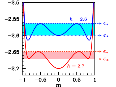
Figure 3: (Color online) The function $f_{-}(m)$ for $s=1$, $\gamma=1$ and two values of $h$: $h=2.6$ (blue curve on top) and $h=2.7$ (red curve at bottom), which correspond to values just across the first order phase transition, $h_{c}\simeq 2.63113$. Even in these cases there is a threshold energy $\epsilon_{*}$ above which all eigenstates are symmetry invariant. In addition, there is coexistence of symmetry breaking and symmetry invariant eigenstates in the interval $[\varepsilon_{*},\epsilon_{*}]$.

A phase transition within a given subspace may on the contrary still occur in the microcanonical ensemble, i.e. at fixed total energy. Without repeating the calculations of Ref. Bapst and Semerjian, 2012, we just recall that the allowed eigenvalues $E=N\epsilon$ of $\mathcal{H}_{\mathbf{0}}$, Eq. (3), in the semiclassical $N\to\infty$ limit are restricted within the interval

$$\min_{m}\Big{(}f_{-}(m,s)\Big{)}\leq\epsilon\leq\text{Max}_{m}\Big{(}f_{+}(m,s)\Big{)},$$ (21)

where

$$f_{\pm}(m,s) = -\gamma s^{2}\,m^{2}-s^{4}\,m^{4}\pm h\,s\,\sqrt{1-m^{2}}\,,.$$

Conversely, eigenstates with eigenvalues $E=N\epsilon$ and total spin $S$ will have components on states $\mid S^{z},S\rangle$, where $S=s\,N/2$ and $S^{z}=S\,m$, only for values of $m$ such that $f_{-}(m,s)\leq\epsilon$ and $f_{+}(m,s)\geq\epsilon$. Outside that interval, the eigenfunctions decay exponentially fast in $N$.

In Fig. 2 we show $f_{+}(m,s)$ and $f_{-}(m,s)$ for $s=1$, $\gamma=1$ and $h=1.9$, which corresponds to the case in Eq. (13) with an ordered ground state. As discussed in Refs. Bapst and Semerjian, 2012, all eigenstates with eigenvalues $\epsilon\leq\epsilon_{*}$, (see figure) are doubly degenerate and symmetry non-invariant, while those with $\epsilon>\epsilon_{*}$ are non-degenerate and symmetry invariant. There is therefore a symmetry breaking edgeMazza and Fabrizio (2012) defined as the critical energy $E_{*}=N\,\epsilon_{*}$ above which symmetry is restored in the microcanonical ensemble. More interesting is the behavior in the coexistence region of Eq. (17). In Fig. 3 we show $f_{-}(m,s)$ still for $s=1$ and $\gamma=1$, and for two different values of $h=2.6$ and $h=2.7$ on both sides of the first order phase transition. In this case there are two relevant energy thresholds. For instance, when $h=2.6$, on the ferromagnetic side, for $\epsilon\leq\varepsilon_{*}$ all eigenstates are symmetry breaking. In the region $\varepsilon_{*}\leq\epsilon\leq\epsilon_{*}$ there are both symmetry non-invariant and invariant eigenstates. Finally, when $\epsilon>\epsilon_{*}$, only symmetry invariant eigenstates exist. On the contrary, on the paramagnetic side of the transition at $h=2.7$, the low energy eigenstates, $\epsilon\leq\varepsilon_{*}$, are symmetry invariant, while for $\varepsilon_{*}\leq\epsilon\leq\epsilon_{*}$ there is coexistence.

The semiclassical equation of motion for the magnetization $m$ is equivalent to the Hamilton-Jacobi equation corresponding to the classical HamiltonianSciolla and Biroli (2011); Mazza and Fabrizio (2012)

$$\mathcal{H}(m,\phi)=-\gamma\,s^{2}\,m^{2}-s^{4}\,m^{4}-h\,s\,\sqrt{1-m^{2}}\;\cos 2\phi,$$ (22)

with $m$ and $\phi$ conjugate variables. Since the energy is conserved, if initially the state has energy $\epsilon$ then

$$\dot{m}=\mp 2\sqrt{\Big{(}f_{+}(m,s)-\epsilon\Big{)}\Big{(}\epsilon-f_{-}(m,s)\Big{)}}\;,$$ (23)

which explicitly shows that, if $\epsilon\geq\epsilon_{*}$, even if initially $m(t=0)\not=0$, during the evolution $m(t)$ oscillates between $\pm m_{0}$ where $f_{-}(\pm m_{0},s)=\epsilon$, so that its time average

$$\overline{m}(\tau)=\frac{\displaystyle 1}{\displaystyle\tau}\int_{0}^{\tau}\,dt\,m(t),$$

vanishes over a period $\tau$.

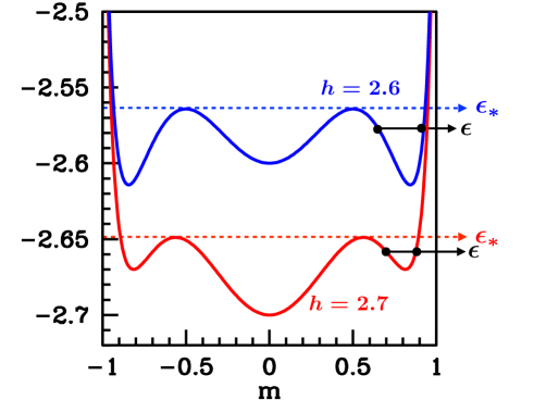
Figure 4: (Color online) As in Fig. 3, showing two initial conditions identified by the energy $\epsilon$. In both cases the magnetization will oscillate between the two black points shown in the figure.

On the contrary, if initially $m(0)$ falls within one of the $f$-valleys at finite magnetisation, see Fig. 4, its time average remains finite until $\epsilon\leq\epsilon_{*}$, even if the actual minimum is at $m=0$, such as for $h=2.7$. As soon as $\epsilon$ exceeds $\epsilon_{*}$, the time average suddenly jumps to zero, signalling a first order dynamical restoration of symmetry.

III.1 A non-equilibrium pathway

Let us consider the Hamiltonian $\mathcal{H}(m,\phi)$ at $\gamma=1$ in the coexistence region for $h=2.631131\gtrsim h_{c}$, where the ground state is disordered, i.e. $m=0$, but there exists a metastable state at $m\simeq 0.836$, and add a perturbation

$$\delta\mathcal{H}(\phi,t)=-\mu\,\theta\big{(}\tau-t\big{)}\,\phi,$$ (24)

which displaces the magnetisation and acts for a finite time $\tau$. The semiclassical equations of motion now read

$$\dot{m}(t) = -\frac{\displaystyle\partial\mathcal{H}(m,\phi)}{\displaystyle\partial\phi}+\mu\,\theta\big{(}\tau-t\big{)},$$ (25)

$$\dot{\phi}(t) = \frac{\displaystyle\partial\mathcal{H}(m,\phi)}{\displaystyle\partial m}-\eta\,\phi(t),$$ (26)

where $\eta$ is the strength of a dissipative process that we need to add in order to force relaxation to a steady state.

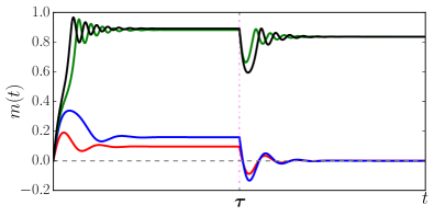
Figure 5: (Color online) Dynamical evolution given by Eq. (25) and (26) for increasing $\mu=0.4,~{}0.6,~{}0.7$ and 0.8 from bottom to top, with the dissipation parameter $\eta=1.5$.

In Fig. 5 we show the non-equilibrium time-dependent magnetisation as derived by solving Eqs. (25) and (26). At the initial time the system is in the equilibrium configuration, $m(0)=\phi(0)=0$, and is let evolve in the presence of the perturbation Eq. (24) for increasing $\mu$, curves from bottom to top. We observe that whereas for small $\mu$ the system returns to the ground state as expected after the switching off of the $\mu$ term, above a threshold value of $\mu$ it remains trapped into the metastable state corresponding to a side $f$-valley, a trapping all the more suggestive given such a simple and dissipative model. This trapping is intimately connected with spatial uniformity, as we shall see.

IV Space Inhomogeneity: Interface Phenomena

The dynamical evolution depicted in Fig. 4 for $h=2.7$, or that in Fig. 5, where the system ends up trapped in a metastable symmetry breaking phase is appealing but not physical. In real systems, bubbles of the stable disordered phase nucleate by quantum fluctuations, and eventually grow at the expense of the metastable long-range-ordered phase, finally destroying it . Quantum nucleation has been extensively studied in a wide variety of contexts, ranging from cosmology to quantum liquids, and the literature on the argument is so vast that it is practically impossible to track it after the seminal works by Coleman Coleman (1977) and by Voloshin, Kobzarev and Okun’ Voloshin et al. (1974). In the case of macroscopic magnets, which is more pertinent to the present work, we may refer to two review articles, Refs. STAMP et al., 1992 and Owerre and Paranjape, 2015, and references therein.

Our aim here will not be to explore quantum nucleation in the toy model Eq. (1), whose overall phenomenology is not going to differ much from the models studied for instance in Ref. STAMP et al., 1992. However, nucleation implies a quantum interface between the stable and the metastable phase. The physics of this type of interface, even when static, demands a separate study. Its results could be of additional interest in view of our conjectured connection with electronic models displaying a zero-temperature first-order Mott transition.

We already mentioned that the effective theory which describes within the Gutzwiller approximation the single-band Mott transition is the Ising model Eq. (1) with $J^{(4)}=0$. In this particular context, Borghi et al. studied Borghi et al. (2009, 2010) several quantum interfaces of direct physical interest, for instance between a Mott insulator and a metal, or between a correlated metal and the vacuum. In the latter case it was found that a poorly metallic, nearly insulating dead layer appears at the metal surface, with a thickness controlled by the Mott transition correlation length. Because in that model the Mott transition is continuous, the correlation length can, close to the transition, be much larger than characteristic electronic length scales of the metal, i.e. the Fermi wavelength or the screening length. An anomalously thick superficial dead layer devoid of measurable quasiparticle weight was indeed observed by surface sensitive photoemission in V₂O₃ Rodolakis et al. (2009). However the Mott transition in V₂O₃ is first order, hence it is not guaranteed that the results of Borghi et al. Borghi et al. (2009, 2010), valid for a continuous transition, are representative.

Here we shall repeat the analyses of Refs. Borghi et al., 2009 and Borghi et al., 2010 with $J^{(4)}\not=0$ and highlight the novel features brought by the first order character of the transition. Specifically we shall study the situation, schematically drawn in Fig. 6, of a semi-infinite slab, $z\in[0,\infty]$, constrained to lie at the surface, $z=0$, in the metastable minimum with $m(z=0)=m_{0}$. Deep in the bulk the slab flows back to its equilibrium phase, i.e. the absolute potential minimum at $m=m_{\infty}$, so that $m(z\to\infty)=m_{\infty}$. As discussed in section II.2 the specific case of $m_{0}=0$ and $m_{\infty}$ finite should translate precisely in an interface between the vacuum ($m_{0}=0$) and a correlated metal ($m_{\infty}\not=0$).

As expected close to any first order phase transition, such as melting, Tartaglino et al. (2005) we will find that the metastable phase wets the surface layers. That is, by moving from the ”disordered” surface at $z$ = 0 into the ”ordered” bulk, the bulk order parameter is not recovered in a simple exponential manner as in the second order case studied by Refs. Borghi et al., 2009. Instead, a disordered film of small but finite thickness will form at the surface, inside which $m(z)\sim m_{0}$, subsequently turning from $m_{0}$ to $m_{\infty}$ at the ”wetting interface”. We shall define the position of the wetting interface with $z=z_{*}$ such that $m(z_{*})$ corresponds to the top of the barrier between the two minima, as sketched in Fig. 6. In what follows, we will start with the classical equilibrium configuration and then study quantum fluctuations of this wetting interface.

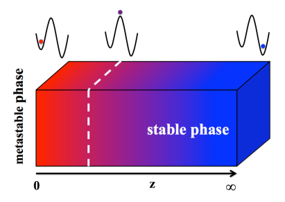
Figure 6: The surface phenomena that we investigate. A semi-infinite slab $z\in[0,\infty]$ is constrained to lie at the surface $z=0$ in the metastable minimum, while, deep in the bulk, $z\gg 1$, it recovers its equilibrium phase. The metastable phase wets the surface layers. At a particular $z=z_{*}$ the system finds itself on the top of the potential barrier, as sketched in figure, which we shall associate with the position of the wetting interface.

IV.1 The continuous limit of the slab

In order to study interface phenomena we must abandon the simple model $\mathcal{H}_{0}$, which cannot describe spatial inhomogeneities, and consider the whole Hamiltonian $\mathcal{H}_{0}+\delta\mathcal{H}$ in Eq. (1). Alternatively, we may adopt a less rigorous approach and consider the model in a slab geometry. Each layer $i=1,\dots,L$ in the slab, with number of sites $A\to\infty$, is described by the infinitely connected Hamiltonian $\mathcal{H}_{0}$ in the $S=A/2$ sector, and it is coupled to its adjacent layers $i-1$ and $i+1$ by a quadratic and a quartic term.

Specifically, the Hamiltonian per unit area reads

$$\mathcal{H} = \sum_{i=1}^{L}\mathcal{H}_{0i}-\sum_{i}\,\bigg{[}\gamma_{\perp}\,m_{i}\,m_{i+1}+\tilde{\gamma}_{\perp}m_{i}^{2}\,m_{i+1}^{2}\bigg{]},\;\;\;\;\;$$ (27)

where

$${\mathcal{H}}_{0i}=-\gamma\,m_{i}^{2}-\tilde{\gamma}\,m_{i}^{4}-h\,\sqrt{1-m_{i}^{2}}\;\cos 2\phi_{i},$$ (28)

with $-1\leq m_{i}\leq 1$ and $\phi_{i}$ conjugate variables, $\gamma_{\perp}$ and $\tilde{\gamma}_{\perp}$ the strengths of the quadratic and quartic interactions between adjacent layers, respectively. The model thus describes a spin chain where the spin at site $i$ is actually the total spin of the individual layer $i$, hence its magnitude $S=A/2$ is large. Since each layer is infinitely connected, it is also infinitely stiff so that the model by construction cannot describe fluctuations perpendicular to the slab axis.

Taking the continuum limit of Eq. (27) yields the following expression of the Hamiltonian:

$$\mathcal{H} = \int_{0}^{\infty}dz\bigg{[}-(\tilde{\gamma}+\tilde{\gamma}_{\perp})m^{4}(z)-(\gamma+\gamma_{\perp})\,m^{2}(z)+$$

$$- h\sqrt{1-m^{2}(z)}\cos 2\phi(z)+$$

$$- \frac{\gamma_{\perp}}{2}m(z)\,\frac{\partial^{2}m(z)}{\partial z^{2}}-\frac{\tilde{\gamma}_{\perp}}{2}m(z)^{2}\,\frac{\partial^{2}m(z)^{2}}{\partial z^{2}}\bigg{]}$$

$$= C+\int_{0}^{\infty}\!\!dz\bigg{[}\frac{\displaystyle K_{\perp}\big{(}m(z)\big{)}}{\displaystyle 2}\,\left(\frac{\displaystyle\partial m(z)}{\displaystyle\partial z}\right)^{2}+V\big{(}m(z)\big{)}$$

$$\phantom{C+\int_{0}^{\infty}dz\;}+2h\,\sqrt{1-m^{2}(z)}\;\sin^{2}\phi(z)\bigg{]},$$

where, as discussed earlier, we assumed that $m(0)=m_{0}$ and $m(\infty)=m_{\infty}$ are fixed ,

$$C=-\frac{1}{4}\int_{0}^{\infty}dz\,\bigg{[}\gamma_{\perp}\,\frac{\partial^{2}m(z)^{2}}{\partial z^{2}}+\tilde{\gamma}_{\perp}\,\frac{\partial^{2}m(z)^{4}}{\partial z^{2}}\bigg{]},$$

is a constant that depends on the boundary values and which we shall drop hereafter. We defined

$$V(m) = -(\tilde{\gamma}+\tilde{\gamma}_{\perp})\,m^{4}-(\gamma+\gamma_{\perp})\,m^{2}$$ (30)

$$-h\sqrt{1-m^{2}},$$

$$K_{\perp}(m) = \gamma_{\perp}+4\,\tilde{\gamma}_{\perp}\,m^{2}.$$ (31)

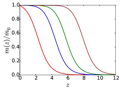
Figure 7: Magnetization $m(z)$, in units of the surface value, as function of the distance from the surface $z$ for different values of $h$ in the case of an ordered wetting layer, namely within the coexistence region where the stable phase is disordered and the ordered phase is metastable. We note the growing thickness of the ordered region as the first order critical point at $h_{c}\simeq 2.63113$ is approached.

In what follows we shall assume Hamiltonian parameters such that the model is within the coexistence region. As mentioned, we choose $m_{\infty}$ as the equilibrium value, which thus corresponds to the absolute minimum of the potential, $V(m)\geq V(m_{\infty})=V_{\infty}$, $\forall m$. For convenience we shift the energy by $-V_{\infty}$, so that the potential turns into

$$V(m)\to V(m)-V_{\infty}\geq 0.$$ (32)

On the other hand, the surface value $m_{0}$ is chosen as the metastable minimum, with potential energy $V(m_{0})-V(m_{\infty})\equiv\Delta V_{0}\geq 0$.

We first study the saddle point configuration that minimises the energy functional Eq. (IV.1). The minimum is obtained when the conjugate momentum is zero, i.e. $\phi(z)=0$, and $m(z)$ satisfies the differential equation:

$$\frac{\delta\mathcal{H}}{\delta m} = \frac{dV(m)}{dm}-K_{\perp}(m)\,m^{\prime\prime}$$ (33)

$$-\frac{\displaystyle 1}{\displaystyle 2}\,K^{\prime}_{\perp}(m)\,m^{\prime}\,{}^{2}=0,$$

with fixed boundary conditions $m(0)=m_{0}$ and $m(\infty)=m_{\infty}$. Eq. (33) admits an integral of motion:

$$I = \frac{\displaystyle K_{\perp}\big{(}m(z)\big{)}}{\displaystyle 2}\;m^{\prime}(z)^{2}-V\big{(}m(z)\big{)},$$ (34)

and corresponds to the energy of a particle in the inverted potential $-V(m)$. Coleman (1977) The lowest energy trajectory is that one with lowest $I$, which, because $I\geq-V\big{(}m(z)\big{)}$, $\forall z$, and through the definition Eq. (32), must correspond to $I=0$. We thus obtain an implicit formula for $m(z)$:

$$\int_{m_{0}}^{m(z)}dm\;\sqrt{\frac{\displaystyle K_{\perp}(m)}{\displaystyle 2\,V(m)}}=\pm z,$$ (35)

where the $+$ refers to the case $m_{0}<m_{\infty}$, and the $-$ to the opposite case.

We thus have all elements required to study the two different, but specular phenomena:

• Ordered wetting layer – the bulk is disordered, $m_{\infty}=0$, but the surface is constrained to be ordered, $m_{0}\not=0$. This case should be relevant to an interface between a metal and a Mott insulator. In section IV.3 we shall discuss a better modeling of such situation.

• Disordered wetting layer – This is the opposite case of an ordered bulk, $m_{\infty}\not=0$, and the surface forced to be disordered, $m_{0}=0$. This should be representative of an interface between the vacuum and a correlated metal.

IV.2 Wetting

In Fig. 7 and Fig. 8 we show the numerical solution of Eq. (35) in both cases of either ordered or of disordered wetting layers, respectively, for the model of Eq. (IV.1) with parameters $\gamma=\tilde{\gamma}=\gamma_{\perp}=\tilde{\gamma}_{\perp}=1/2$, in which case the coexistence region is $2\leq h\leq\sqrt{8}\simeq 2.83$, with the first order transition at $h=h_{c}\simeq 2.63113$. In both cases a wetting layer forms at the surface, its thickness growing as the first order quantum phase transition is approached at $h_{c}$.

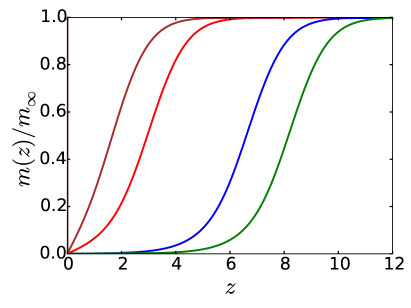
Figure 8: Magnetization $m(z)$, in units of the bulk value, as function of the distance $z$ from the surface for different values of $h$ in the case of a disordered wetting layer, namely within the coexistence region where the stable phase is ordered and the disordered phase is metastable. Note the growing thickness of the disordered region as the first order transition point at $h_{c}\simeq 2.63113$ is approached.

The critical properties of classical wetting at an interface have been extensively studied over many years, see e.g. Refs. Cahn, 1977; Lipowsky, 1982; Brézin et al., 1983a; Fisher and Huse, 1985; de Gennes, 1985; Lipowsky and Fisher, 1987; Jin and Fisher, 1993; Bonn and Ross, 2001; Tartaglino et al., 2005; Parry et al., 2008; Bonn et al., 2009; Parry and Rascón, 2009; Indekeu, 2010; Rath et al., 2011; Jakubczyk, 2012, which is not at all an exhaustive list. Here we will rederive some simple results in order to set up the terminology for the subsequent discussion of quantum fluctuations applicable to our case.

We assume the wetting interface to be located at $z=z_{*}$ when $m(z)$ reaches the top of the barrier that separates the two minima of $V(m)$, see Fig. 6. Moreover, we assume that the width $W$ of the interface is the distance needed to go from the inflection point $m_{1}$ at the left of $m_{*}$ to that at the right, $m_{2}$, see Fig. 9 where for simplicity we take $m_{0}<m_{\infty}$, i.e. the case of a disordered wetting layer. Through Eq. (35) we find that

$$W=\int_{m_{1}}^{m_{2}}dm\;\sqrt{\frac{\displaystyle K_{\perp}(m)}{\displaystyle 2\,V(m)}}.$$ (36)

The thickness of the wetting layer can be defined as the distance required to reach $m_{1}$ from the surface value $m_{0}$, i.e.

$$l=\int_{m_{0}}^{m_{1}}dm\;\sqrt{\frac{\displaystyle K_{\perp}(m)}{\displaystyle 2\,V(m)}}.$$ (37)

Close to the first order transition, $h\to h_{c}$, the integral is dominated by the region close to $m_{0}$. If we approximate

$$V(m)\simeq\Delta V_{0}+\frac{\displaystyle\kappa_{0}}{\displaystyle 2}\,\big{(}m-m_{0}\big{)}^{2},$$

where $\kappa_{0}>0$, $K_{\perp}(m)\simeq K_{\perp}(m_{0})$, and $\Delta V_{0}>0$ vanishing linearly when $h\to h_{c}$, we find

$$l \simeq \sqrt{\frac{\displaystyle K_{\perp}(m_{0})}{\displaystyle\kappa_{0}}}\;\sinh^{-1}\sqrt{\frac{\displaystyle\kappa_{0}}{\displaystyle 2\Delta V_{0}}}\;\big{(}m_{1}-m_{0}\big{)}$$ (38)

$$\simeq \sqrt{\frac{\displaystyle K_{\perp}(m_{0})}{\displaystyle\kappa_{0}}}\;\ln\left(2\;\sqrt{\frac{\displaystyle\kappa_{0}}{\displaystyle 2\Delta V_{0}}}\;\big{(}m_{1}-m_{0}\big{)}\right)$$

$$\simeq -\frac{\displaystyle 1}{\displaystyle 2}\sqrt{\frac{\displaystyle K_{\perp}(m_{0})}{\displaystyle\kappa_{0}}}\;\ln\big{|}h-h_{c}\big{|}.$$

The thickness of the wetting layer diverges logarithmically as the first order bulk transition is approached, $\Delta V_{0}\to 0$, thus displaying a surface critical phenomenon despite the discontinuous nature of the bulk transition. Cahn (1977); Lipowsky (1982) Within the same approximation and for $z<l$,

$$m(z)\simeq m_{0}+\sqrt{\frac{\displaystyle 2\Delta V_{0}}{\displaystyle\kappa_{0}}}\;\sinh\sqrt{\frac{\displaystyle\kappa_{0}}{\displaystyle K_{\perp}(m_{0})}}\;z.$$ (39)

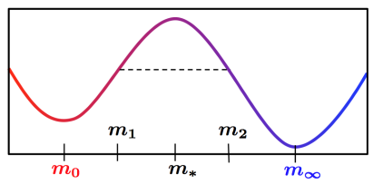
Figure 9: Values of the magnetization relevant to define the wetting layer. We assume that the wetting interface has a width that corresponds to the distance required to go from the two inflection points $m_{1}$ and $m_{2}$. The wetting layer is defined as the distance to reach $m_{1}$ starting from the surface value $m_{0}$.

On the contrary, when $z\gg l$, hence $m(z)\simeq m_{\infty}$, we can approximate

$$V(m)\simeq\frac{\displaystyle\kappa_{\infty}}{\displaystyle 2}\,\big{(}m-m_{\infty}\big{)}^{2},$$

so that

$$m_{\infty}-m(z)\sim\exp\bigg{(}-\sqrt{\frac{\displaystyle\kappa_{\infty}}{\displaystyle K_{\perp}(m_{\infty})}}\;z\bigg{)}.$$ (40)

We observe that

$$\xi_{0} = \sqrt{\frac{\displaystyle K_{\perp}(m_{0})}{\displaystyle\kappa_{0}}},$$ (41)

$$\xi_{\infty} = \sqrt{\frac{\displaystyle K_{\perp}(m_{\infty})}{\displaystyle\kappa_{\infty}}},$$ (42)

are precisely the bulk correlation lengths in the metastable and stable phases, respectively, so that

$$l\simeq\xi_{0}\;\ln\big{|}h-h_{c}\big{|}.$$ (43)

IV.3 A model for a metal-Mott insulator interface

If we aim to model a metal-Mott insulator interface, where, as mentioned, the Mott insulator and the metal translate into the paramagnetic and ferromagnetic phases of the Hamiltonian Eq. (IV.1), respectively, it is convenient to consider a slightly different interface problem, introduced by Cahn back in 1977 Cahn (1977) and by now the paradigm of classical wetting transitions.

In that model, the paramagnetic, i.e. Mott-insulating, slab is still described by Eq. (IV.1) with a stable minimum at $m_{\infty}=0$, but one assumes the surface layer at $z=0$ to be coupled to a very stiff ferromagnet, i.e. a very good metal, whose magnetisation $m_{\text{metal}}\simeq 1$ is therefore not affected by the slab. The coupling is thus modelled by the surface potential Cahn (1977)

$$\Phi\big{(}m_{s}\big{)}=-\lambda_{\perp}\,\Big{(}m_{s}\,m_{\text{metal}}+m_{s}^{2}\,m_{\text{metal}}^{2}\Big{)},$$ (44)

where we denote $m(0)=m_{s}$ and, as mentioned, $m_{\text{metal}}\simeq 1$ is constant. As before we start by the saddle point configuration where the conjugate field $\phi(z)=0$ and $m(z)$ is the solution of Eq. (33), or, through Eq. (34) with $I=0$, of

$$m^{\prime}(z)=-\sqrt{\frac{\displaystyle 2V\big{(}m(z)\big{)}}{\displaystyle K_{\perp}\big{(}m(z)\big{)}}}\;,$$ (45)

where we now choose the minus sign since $m(z)$ decreases with $z$. The difference is that the surface magnetisation $m(0)=m_{s}$, i.e. the boundary condition of Eq. (45), must now be determined by minimising the total energy

$$E\big{(}m_{s}\big{)} = \Phi\big{(}m_{s}\big{)}+\int_{0}^{\infty}\!\!dz\bigg{[}\frac{\displaystyle K_{\perp}\big{(}m(z)\big{)}}{\displaystyle 2}\,\left(\frac{\displaystyle\partial m(z)}{\displaystyle\partial z}\right)^{2}$$

$$+V\big{(}m(z)\big{)}\bigg{]}=\Phi\big{(}m_{s}\big{)}+2\,\int_{0}^{\infty}\!\!dzV\big{(}m(z)\big{)}$$

$$= \Phi\big{(}m_{s}\big{)}+\int_{0}^{m_{s}}\!\!dm\;\sqrt{2\,K_{\perp}(m)\,V(m)}$$

$$= \int_{0}^{m_{s}}\!\!dm\,\bigg{[}\sqrt{2\,K_{\perp}(m)\,V(m)}-\Big{(}-\Phi^{\prime}(m)\Big{)}\bigg{]},$$

where the last equation holds since $\Phi(0)=0$. The surface value $m_{s}$ thus satisfies the equation

$$\sqrt{2\,K_{\perp}(m_{s})\,V(m_{s})}=-\Phi^{\prime}(m_{s}),$$ (47)

which is graphically shown in Fig. 10 for increasing values of $\lambda_{\perp}>0$.

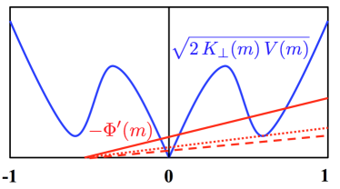
Figure 10: Graphical solution of Eq. (47). The blue curve is $\sqrt{2\,K_{\perp}(m_{s})\,V(m_{s})}$, while the red straight lines represent $-\Phi^{\prime}(m_{s})$ for increasing values of $\lambda_{\perp}$, from bottom to top.

We observe that for small $\lambda_{\perp}$, dashed line in the figure, there are only two crossing points, at the left and at the right of $m=0$, the latter a minimum of the energy and the former a maximum. Only above a threshold, shown as a dotted line, two other extrema appear. In that case there are two minima, denoted as $m_{\text{low}}$ and $m_{\text{high}}$ in Fig. 11.

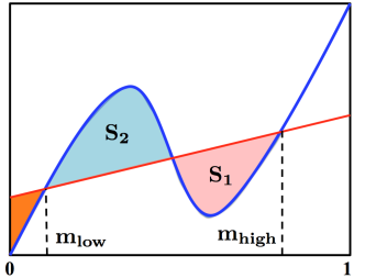
Figure 11: The two minima $m_{\text{low}}$ and $m_{\text{high}}$ for the surface magnetisation $m_{s}$ above the threshold value of the coupling to the ferromagnet. The total energy is given by the shaded areas where the pink and orange ones are taken with negative sign and the cyan one with positive sign.

Through the last expression in Eq. (IV.3), we readily obtain that the energy of the solution $m_{s}=m_{\text{low}}$ is minus the orange shaded area shown in Fig. 11, while that of $m_{s}=m_{\text{high}}$ is the cyan shaded area, $S_{2}$ in the figure, minus the sum of the orange plus the pink, $S_{1}$ in the figure, areas. In other words

$$E\big{(}m_{\text{low}}\big{)}-E\big{(}m_{\text{high}}\big{)}=S_{1}-S_{2}\equiv S,$$ (48)

where $S$ is the so-called spreading coefficient, see e.g. Ref. de Gennes, 1985. It follows that, if $S<0$, the absolute minimum is obtained for $m_{s}=m_{\text{low}}$, which corresponds to what is called partial wetting. de Gennes (1985) On the contrary, when $S>0$ the absolute minimum has surface magnetisation $m_{s}=m_{\text{high}}$ which corresponds to complete wetting. $S=0$ signals a first order transition between the two solutions, where the surface magnetisation jumps discontinuously from $m_{\text{low}}$ to $m_{\text{high}}$.

If we still denote as $m_{0}<m_{\text{high}}$ the metastable ferromagnetic, i.e. metallic, minimum of $V(m)$, the thickness of the wetting layer increases with respect to $l$, Eq. (38), i.e. to the situation discussed in section IV.2, by

$$\delta l=\int_{m_{0}}^{m_{\text{high}}}\,dm\,\sqrt{\frac{\displaystyle K_{\perp}(m)}{\displaystyle 2V(m)}}\;,$$ (49)

which also diverges logarithmically as the bulk transition is approached.

IV.4 Fluctuations in the harmonic approximation

The distiguishing feature of quantum wetting from its classical counterpart is represented by quantum fluctuations. We therefore add quantum fluctuations to the saddle point solution discussed in section IV.2 within the harmonic approximation. We start from the Hamiltonian:

$$\mathcal{H} = \int_{0}^{L}\!\!dz\Bigg{[}\frac{\displaystyle K_{\perp}\big{(}m(z)\big{)}}{\displaystyle 2}\,\left(\frac{\displaystyle\partial m(z)}{\displaystyle\partial z}\right)^{2}+V\big{(}m(z)\big{)}$$ (50)

$$\phantom{\int_{0}^{L}\!\!dz\Bigg{[}}+2h\,\sqrt{1-m^{2}(z)}\;\sin^{2}\phi(z)\Bigg{]},$$

this time defined within the interval $z\in[0,L]$, where $L$ will be sent to infinity afterwards. The functional Eq. (50) is minimized by $\phi=0$ and by the solution of Eq. (34) with $I=0$, which we shall denote as $m_{\text{sp}}(z)$, with boundary conditions $m_{\text{sp}}(0)=m_{0}$ and $m_{\text{sp}}(L\to\infty)=m_{\infty}$. We perform a change of variable $m(z)\to q(z)$ where

$$\sqrt{K_{\perp}(m)}\;dm=dq,$$ (51)

so that the saddle point trajectory $q_{\text{sp}}(z)$ satisfies

$$q^{\prime\prime}_{\text{sp}}(z) = \frac{\displaystyle\partial V\big{(}m(q)\big{)}}{\displaystyle\partial q}_{\big{|}q=q_{\text{sp}}(z)}$$

$$= \left(\frac{\displaystyle 1}{\displaystyle\sqrt{K_{\perp}(m)}}\;\frac{\displaystyle\partial V(m)}{\displaystyle\partial m}\right)_{\big{|}m=m\big{(}q_{\text{sp}}(z)\big{)}},$$

$$\frac{\displaystyle q^{\prime}_{\text{sp}}(z)^{2}}{\displaystyle 2} = V\Big{(}m\big{(}q_{\text{sp}}(z)\big{)}\Big{)},$$ (53)

from which it follows that $q^{\prime\prime}_{\text{sp}}(0)=q^{\prime\prime}_{\text{sp}}(L)=0$. Moreover, because the potential has been rigidly shifted in such a way that the absolute minimum at $z=L$ is zero, it also follows that $q^{\prime}_{\text{sp}}(L)=0$.

If we vary $q(z)$ at fixed boundary conditions, i.e.

$$q(z)=q_{\text{sp}}(z)+\psi(z),$$ (54)

with small $\psi(z)$ such that $\psi(0)=\psi(L)=0$, which corresponds to

$$m(z)=m_{\text{sp}}(z)+\sqrt{\frac{\displaystyle 1}{\displaystyle K_{\perp}\big{(}m_{\text{sp}}(z)\big{)}}}\;\psi(z),$$

the energy functional in Eq. (50), up to second order in $\psi(z)$ and $\phi(z)$, changes into

$$\mathcal{H} \simeq E\big{[}m_{\text{sp}}(z)\big{]}+\frac{\displaystyle 1}{\displaystyle 2}\,\int_{0}^{\infty}dz\,\Bigg{[}\Big{(}\partial\psi(z)\Big{)}^{2}$$ (55)

$$+U^{(2)}(z)\,\psi(z)^{2}+4h\,\sqrt{1-m_{\text{sp}}^{2}(z)\,}\;\phi(z)^{2}\Bigg{]},\qquad$$

where

$$U^{(n)}(z)=\frac{\displaystyle\partial^{n}V\big{(}m(q)\big{)}}{\displaystyle\partial q^{n}}_{\big{|}q=q_{\text{sp}}(z)}.$$ (56)

The potential $U^{(2)}(z)$ has the following limiting values

$$U^{(2)}(z\to 0) \to \frac{\displaystyle\kappa_{0}}{\displaystyle K_{\perp}(m_{0})}=\xi_{0}^{-2}>0,$$

$$U^{(2)}(z\to L) \to \frac{\displaystyle\kappa_{\infty}}{\displaystyle K_{\perp}(m_{\infty})}=\xi_{\infty}^{-2}>0,$$

and has a negative minimum $-U_{*}<0$ approximately at $z=z_{*}$; in other words it describes a potential well centered around the wetting interface.

IV.4.1 An auxiliary eigenvalue problem

Let us consider the auxiliary problem Coleman (1985); Brézin et al. (1983b) that consists of solving the following Schrœdinger eigenvalue equation in $z\in[-L,L]$ with vanishing conditions at $z=\pm L$:

$$\bigg{(}-\frac{\displaystyle\partial^{2}}{\displaystyle\partial z^{2}}+U(z)\bigg{)}\,\psi_{n}(z)=\epsilon_{n}\,\psi_{n}(z),$$ (57)

where

$$U(z)=\left\{\begin{array}[]{cc}\displaystyle U^{(2)}(z)&\displaystyle\mbox{when }z\geq 0\\ \displaystyle U^{(2)}(-z)&\displaystyle\mbox{when }z<0\end{array}\right..$$ (58)

The potential $U(z)$ thus describes two symmetric wells centered roughly at $\pm z_{*}$. The eigenstates of Eq. (57) can be always chosen real and distinguished into even, $\psi^{\text{even}}_{n}(z)=\psi^{\text{even}}_{n}(-z)$, and odd, $\psi^{\text{odd}}_{n}(z)=-\psi^{\text{odd}}_{n}(-z)$, with eigenvalues $\epsilon^{\text{even}}_{n}$ and $\epsilon^{\text{odd}}_{n}$, respectively, with $n\geq 0$. By continuity of the wavefunction and its first derivative at the origin, $\partial\psi^{\text{even}}_{n}(0)=0$ and $\psi^{\text{odd}}_{n}(0)=0$, while, by construction, $\psi^{\text{even}}_{n}(\pm L)=\psi^{\text{odd}}_{n}(\pm L)=0$. We now note that the even-parity wavefunction defined as $\psi(z)=q^{\prime}_{\text{sp}}(z)$ for $z>0$, and $\psi(z)=q^{\prime}_{\text{sp}}(-z)$ for $z<0$, is a solution of Eq. (57) with vanishing eigenvalue that satisfies all appropriate boundary conditions. Since it is nodeless, it is actually the ground state of Eq. (57): $\psi(z)\equiv\psi^{\text{even}}_{0}(z)$ with eigenvalue $\epsilon^{\text{even}}_{0}=0$. It thus follows that, since all eigenvalues in the odd parity sector must be necessarily greater than the ground state energy, then $\epsilon^{\text{odd}}_{n}>0$, $\forall n\geq 0$; the saddle point is stable to fluctuations.

Now suppose the system is very close to the first order transition, i.e. $\Delta V_{0}\ll 1$. In this case the two potential wells in $U(z)$ are very far apart and we can safely assume that the ground state $\psi^{\text{even}}_{0}(z)$, with energy $\epsilon^{\text{even}}_{0}=0$, is the symmetric combination of the ground state wavefunctions of each well, while the first excited state is the antisymmetric combination, hence is the lowest energy state in the odd sector. The two states are split by the quantum tunneling amplitude between the two wells. Within the WKB approximation we can estimate that energy splitting as

$$\epsilon^{\text{odd}}_{0}-\epsilon^{\text{even}}_{0} = \epsilon^{\text{odd}}_{0}\simeq 2\,\frac{\displaystyle\sqrt{U_{*}}}{\displaystyle W}\;\text{e}^{-2\,l/\xi_{0}}$$ (59)

$$\simeq 2\,\frac{\displaystyle\sqrt{U_{*}}}{\displaystyle W}\;\big{|}h-h_{c}\big{|}\,,$$

which is therefore the leading term of the lowest eigenvalue in the odd sector.

Figure 12: The lowest energy wavefunction $\psi^{\text{odd}}_{0}(z)$ in the odd sector for $h=2.6311298<h_{c}$ very close to the transition, $\Delta V_{0}=2.3\,10^{-7}$. In the inset we show the saddle point magnetization profile $m_{\text{sp}}(z)$.

In Fig. 12 we plot $\psi^{\text{odd}}_{0}(z)$ in the case of a disordered wetting layer very close to the first order transition, when $\Delta V_{0}=2.3\,10^{-7}$.

We believe that, besides the above two states, with energies $\epsilon^{\text{even}}_{0}$ and $\epsilon^{\text{odd}}_{0}$, there are no other eigenstates that are bound within the potential wells. In other words, all other eigenstates have energy greater than $\text{min}\big{(}\xi_{0}^{-2},\xi_{\infty}^{-2}\big{)}$ and are not localized on the wetting interface. We have no rigorous proof of the above statement, even though we find it is confirmed by the semiclassical WKB quantization rule.

To conclude, we note that the existence of a zero energy mode of the Hamiltonian Eq. (57) could be anticipated. Indeed, if we consider the magnetisation profile $m_{\text{sp}}(z-\epsilon)$, with $\epsilon\ll 1$, which corresponds to $\delta q(z)\simeq-\epsilon\,q^{\prime}_{\text{sp}}(z)=-\epsilon\,\psi^{\text{even}}_{0}(z)$, i.e. just to the zero-energy mode, the energy changes into

$$\mathcal{H}(\epsilon)=\int_{-\epsilon}^{\infty}dz\,2\,V\big{(}m_{\text{sp}}(z)\big{)},$$

whose second derivative with respect to $\epsilon$ indeed vanishes

$$\frac{\displaystyle\partial^{2}\mathcal{H}(\epsilon)}{\displaystyle\delta\epsilon^{2}}=-2\frac{\displaystyle\partial V\big{(}m_{\text{sp}}(z)\big{)}}{\displaystyle\partial z}_{\big{|}z=0}=0.$$

IV.4.2 Explicit expression of quantum fluctuations

We now expand $\psi(z)$ and $\phi(z)$ in Eq. (55) in a complete basis within the interval $z\in[0,L]$ with vanishing conditions, which we can take as the set of odd eigenstates of Eq. (57),

$$m(z) = m_{\text{sp}}(z)+\frac{\displaystyle 1}{\displaystyle\sqrt{K_{\perp}(m_{\text{sp}}(z))}}\;\psi(z)$$

$$= m_{\text{sp}}(z)+\sqrt{\frac{\displaystyle 2}{\displaystyle K_{\perp}(m_{\text{sp}}(z))}}\;\sum_{n}\,x_{n}\,\psi^{\text{odd}}_{n}(z),$$

$$\phi(z) = \sqrt{2\,K_{\perp}(m_{\text{sp}}(z))}\;\sum_{n}\,p_{n}\,\psi^{\text{odd}}_{n}(z),$$ (61)

where $[x_{n},p_{m}]=i\,\delta_{nm}$ so that

$$\big{[}m(z),\phi(z^{\prime})\big{]}=i\,\delta(z-z^{\prime}),$$

are indeed conjugate variables. It follows that the Hamiltonian Eq. (55) becomes

$$\mathcal{H}-E\big{[}m_{\text{sp}}(z)\big{]}=+\frac{1}{2}\,\sum_{n}\,\epsilon^{\text{odd}}_{n}\,x_{n}^{2}+\gamma^{\text{odd}}_{nn}\,p_{n}^{2}$$

$$\qquad+\frac{1}{2}\,\sum_{n\not=m}\,\gamma^{\text{odd}}_{nm}\,p_{n}\,p_{m},$$ (62)

where

$$\gamma^{\text{odd}}_{nm} = 8h\,\int_{0}^{L}dz\,\bigg{[}K_{\perp}\big{(}m_{\text{sp}}(z)\big{)}\,$$

$$\phantom{8h\,\int_{0}^{L}dz\;\;\;\;}\,\sqrt{1-m_{\text{sp}}(z)^{2}\,}\;\psi_{n}^{\text{odd}}(z)\psi_{m}^{\text{odd}}(z)\bigg{]}.$$

Since $\psi^{\text{odd}}_{0}(z)$ is localized on the interface, while $\psi^{\text{odd}}_{n}(z)$ for $n>0$ are extended at least over the whole wetting thickness $l$, the coupling $\gamma^{\text{odd}}_{0n}\sim l^{-1/2}$ vanishes approaching the transition. We can therefore treat it within perturbation theory and obtain for the $n=0$ mode the effective Hamiltonian

$$\mathcal{H}_{0} = \frac{\displaystyle\epsilon^{\text{odd}}_{0}}{\displaystyle 2}\;x_{0}^{2}+\frac{\displaystyle\gamma_{0}}{\displaystyle 2}\;p_{0}^{2}=\omega_{0}\,\Big{(}b^{\dagger}_{0}\,b^{\phantom{\dagger}}_{0}+\frac{1}{2}\Big{)},$$ (63)

where

$$\gamma_{0}\simeq\gamma^{\text{odd}}_{00}+\sum_{n,m>0}\,\gamma^{\text{odd}}_{0n}\;\left(\frac{\displaystyle 1}{\displaystyle\hat{\gamma}}\right)^{-1}_{nm}\,\gamma^{\text{odd}}_{m0},$$

with $\hat{\gamma}$ the symmetric real matrix with elements $\gamma^{\text{odd}}_{nm}$, and $b_{0}$ the bosonic operator that diagonalize the Hamiltonian (63) with eigenvalue

$$\omega_{0}=\sqrt{\epsilon^{\text{odd}}_{0}\,\gamma_{0}\,}\,\simeq\big{|}h-h_{c}\big{|}^{1/2},$$ (64)

which vanishes at the first order point, $h=h_{c}$, when the interface can be translated at no energy cost.

Close to the transition, the static fluctuations of $q(z)$ with respect to the saddle point profile $q_{\text{sp}}(z)$ is dominated by the $n=0$ mode,

$$\big{\langle}\,\Big{(}q(z)-q_{\text{sp}}(z)\Big{)}^{2}\,\big{\rangle}\simeq\frac{\displaystyle\gamma_{0}}{\displaystyle\omega_{0}}\;\psi^{\text{odd}}_{0}(z)^{2}\sim\big{|}h-h_{c}\big{|}^{-1/2},$$ (65)

and grow when $h\to h_{c}$, unlike the fluctuations of the conjugate variable $\phi(z)$. This behaviour simply reflects the unbinding of the wetting interface, whose detailed description would require going beyond the harmonic approximation. We observe that the square root divergence in Eq. (65) differs from the classical result Lipowsky , which, through Eq. (63), predicts a more singular behaviour $\sim 1/\epsilon^{\text{odd}}_{0}\sim\big{|}h-h_{c}\big{|}^{-1}$. Therefore, even though the saddle point has evidently the same critical properties as in the classical case, the quantum fluctuations behave differently from the classical ones.

IV.4.3 Back to the metal-Mott insulator interface

In the case of the metal-Mott insulator interface modelled in section IV.3 through a paramagnet slab supplied by an additional surface potential, the allowed eigenvectors $\psi^{\text{odd}}_{n}(z)$ (we keep using the label ”odd”, though now the wavefunction must not vanish anymore at $z=0$) still satisfy the eigenvalue equation (57) for $z>0$ with the boundary condition

$$\frac{\displaystyle\partial\psi^{\text{odd}}_{n}(0)}{\displaystyle\partial z}=\frac{\displaystyle\partial^{2}\Phi\big{(}m(q)\big{)}}{\displaystyle\partial q^{2}}_{\big{|}q=q_{\text{sp}}(0)}\,\psi^{\text{odd}}_{n}(0),$$ (66)

where $\Phi(m)$ is defined by Eq. (44). We assume the model has complete wetting, i.e. $S>0$, see Eq. (48). Since the second derivative of $\Phi(m)$ at the surface value $m_{s}=m_{\text{high}}$ is negative, the boundary condition Eq. (66) actually corresponds to an attractive $\delta$-function potential

$$\delta U(z)=\delta(z)\,\frac{\displaystyle\partial^{2}\Phi\big{(}m(q)\big{)}}{\displaystyle\partial q^{2}}_{\big{|}q=q_{\text{sp}}(0)}=-U_{s}\,\delta(0),$$

with $U_{s}>0$, that adds to $U(z)$ As before, the wavefunction $\psi(z)\propto q^{\prime}_{\text{sp}}(z)$ is the solution of the Schrœdinger equation with vanishing eigenvalue, but with the ”wrong” boundary condition

$$\psi^{\prime}(0) = q^{\prime\prime}_{\text{sp}}(0)=\frac{\displaystyle\partial V\big{(}m(q)\big{)}}{\displaystyle\partial q}_{\big{|}q=q_{\text{sp}}(0)}$$

$$= -\big{(}2K_{\perp}(m_{s})V(m_{s})\big{)}^{-1/2}\;\frac{\displaystyle\partial V(m)}{\displaystyle\partial m}_{\big{|}m=m_{s}}\;\psi(0),$$

where we recall that

$$\sqrt{2K_{\perp}(m_{s})V(m_{s})}=-\Phi^{\prime}(m_{s}).$$

One easily realises that Eq. (IV.4.3) corresponds to a more attractive $\delta$-function potential at $z=0$, which implies once again that the lowest allowed eigenvalue $\epsilon^{\text{odd}}_{0}$ is positive and vanishes only at the bulk first-order transition.

IV.5 Capillary waves at the interface

So far we have assumed each layer to be infinitely connected, which is equivalent to a flat wetting interface. Let us now relax this assumption and consider the three dimensional Ginzburg-Landau Hamiltonian for the fluctuations, see also the Appendix,

$$\mathcal{H} \simeq E\big{[}m_{\text{sp}}(z)\big{]}+\frac{\displaystyle 1}{\displaystyle 2}\,\int d\mathbf{r}\,\int_{0}^{\infty}dz\,\Bigg{[}\Big{(}\partial\psi(z,\mathbf{r})\Big{)}^{2}$$ (68)

$$+U(z)\,\psi(z,\mathbf{r})^{2}+4h\,\sqrt{1-m_{\text{sp}}^{2}(z)\,}\;\phi(z,\mathbf{r})^{2}$$

$$+K_{||}\,\big{(}\boldsymbol{\nabla}\psi(z,\mathbf{r})\big{)}^{2}\Bigg{]},$$

where $\mathbf{r}$ is the coordinate in the plane of each layer and we added an intra-layer (longitudinal) stiffness term. Assuming translational symmetry within each layer, we can Fourier transform in $\mathbf{r}$ introducing the intra-layer, two-dimensional planar momentum $\mathbf{q}$. If we now parametrize:

$$m(z,\mathbf{q}) = m_{\text{sp}}(z)+\frac{\displaystyle 1}{\displaystyle\sqrt{K_{\perp}(m_{\text{sp}}(z))}}\;\psi(z,\mathbf{q})$$

$$= m_{\text{sp}}(z)+\sqrt{\frac{\displaystyle 2}{\displaystyle K_{\perp}(m_{\text{sp}}(z))}}\;\sum_{n}\,x_{n\mathbf{q}}\,\psi^{\text{odd}}_{n}(z),$$

$$\phi(z,\mathbf{q}) = \sqrt{2\,K_{\perp}(m_{\text{sp}}(z))}\;\sum_{n}\,p_{n,\mathbf{q}}\,\psi^{\text{odd}}_{n}(z),$$ (70)

with the same wavefunctions as before and with

$$\big{[}x_{n,\mathbf{q}},p_{m,-\mathbf{q}^{\prime}}\big{]}=i\,\delta_{nm}\,\delta_{\mathbf{q},\mathbf{q}^{\prime}},$$

we find that the $n=0$ mode is described by the effective Hamiltonian

$$\mathcal{H}_{0} = \frac{\displaystyle 1}{\displaystyle 2}\sum_{\mathbf{q}}\,\Big{(}\epsilon^{\text{odd}}_{0}+K_{||}\,q^{2}\Big{)}\,x_{0\mathbf{q}}\,x_{0-\mathbf{q}}+\gamma_{0}\,p_{0\mathbf{q}}\,p_{0-\mathbf{q}}$$ (71)

$$= \sum_{\mathbf{q}}\,\omega_{0\mathbf{q}}\,\Big{(}b^{\dagger}_{0\mathbf{q}}\,b^{\phantom{\dagger}}_{0\mathbf{q}}+\frac{1}{2}\Big{)},$$

where the eigenvalues

$$\omega_{0\mathbf{q}}=\sqrt{\gamma_{0}\,\Big{(}\epsilon^{\text{odd}}_{0}+K_{||}\,q^{2}\Big{)}\,},$$ (72)

allow defining a longitudinal correlation length

$$\xi_{||} \simeq \sqrt{\frac{\displaystyle K_{||}}{\displaystyle\epsilon^{\text{odd}}_{0}}}\sim\big{|}h-h_{c}\big{|}^{-1/2},$$ (73)

to be compared with $l$ in Eq. (38). We highlight that all other modes with $n>0$ are separated by a finite energy gap, so they cannot provide a finite damping at $T=0$ for the $n=0$ capillary wave. In the spin language, the wetting interface thus binds spin wave excitations that sink down below the gapped bulk continuum and propagate coherently along the interface.

The capillary wave contribution to the static fluctuations of the magnetisation $m(z,\mathbf{r})$ with respect to the saddle point profile $m_{\text{sp}}(z)$

$$\big{\langle}\;\Big{(}m(z,\mathbf{r})-m_{\text{sp}}(z)\Big{)}^{2}\;\big{\rangle}\sim\int d\mathbf{q}\;\frac{\displaystyle\gamma_{0}}{\displaystyle\;\omega_{0\mathbf{q}}\;}\;,$$ (74)

is not singular when $h\to h_{c}$, unlike in the classical finite temperature regime where it diverges logarithmically signalling the roughening of the wetting interface.

V Discussion and Conclusions

We have studied some non-equilibrium as well as some non-homogeneous properties of a quantum Ising model with a four-spin exchange, probably the simplest representative of $Z_{2}$-invariant models that display a first-order quantum phase transition, i.e. a zero temperature symmetry-breaking transition upon varying a Hamiltonian parameter.

First, we studied quantum quenches in the mean-field limit of infinite connectivity, where the corresponding Lipkin-Ising model can be solved exactly. In the coexistence region around the first order transition, we found that out-of-equilibrium the spatially homogeneous system can remain trapped into the metastable phase.

Next, we studied the static but spatially inhomogeneous phenomenon that arises in the presence of an interface that pins the surface into the metastable phase. The latter, as in the classical wetting, extends over a finite length $l$ inside the bulk, which diverges as the first-order transition is approached. Specifically, within mean-field, which should provide the correct critical behavior in $d+1=4$ dimensions, Brézin et al. (1983b) the thickness of the wetting layer diverges logarithmically at the first-order quantum phase transition,

$$l\sim-\ln\big{|}h-h_{c}\big{|},$$ (75)

while the longitudinal fluctuations of the wetting interface are controlled by the correlation length

$$\xi_{||}\sim\big{|}h-h_{c}\big{|}^{-1/2},$$ (76)

and are associated to propagating modes with dispersion

$$\omega_{\mathbf{q}}\propto\sqrt{\xi_{||}^{-2}+q^{2}}\,,$$ (77)

where $\mathbf{q}$ is the momentum parallel to the interface. This branch of excitations localised on the wetting interface lies below the bulk spectrum, which has a finite gap in both ordered and disordered phases. It is therefore a coherent mode at low temperatures that cannot decay in the bulk continuum. At the transition it turns into an acoustic mode $\omega_{\mathbf{q}}\sim q$ that at zero temperature does not lead to diverging fluctuations unlike the classical case at finite temperature.

We hypothesize that the above results should be applicable to quantum first-order Mott transitions, with some interesting consequences. The first is the possibility of nucleating long-lived droplets of a metastable metal inside a stable Mott insulator by external perturbations of finite-duration, which recalls recent experiments Wegkamp et al. (2014); Stojchevska et al. (2014) where signatures of non-thermal metallic phases have been observed after irradiation of Mott insulators by ultra-short laser pulses. Moreover, the observation that VO₂ electric double layer transistors formed at a solid/electrolyte interface show upon superficial charging a bulk-like metallization with an extension much beyond the electrostatic screening length, Okuyama et al. (2014) is strongly suggestive of a metallic wetting layer that forms at the interface.

A more realistic modeling of interface phenomena close to a first order Mott transition must include long-range dispersion forces, ignored in the present treatment. As is well known, Lipowsky (1985); Dietrich and Schick (1985); Dietrich and Napiórkowski (1991); Lipowsky (1984) the classical critical properties of the wetting layer and its thickness are severely affected by long-range dispersion forces. Inclusion of dispersion interaction forces of the van der Waals type, or, equivalently, a proper treatment of the electromagnetic fluctuations implied by the different dielectric functions, $\epsilon_{1}(\omega)$, $\epsilon_{2}(\omega)$ and $\epsilon_{3}(\omega)$ of the exterior of the system, of the metastable and of the stable phases respectively, Dzyaloshinskii et al. (1961); Barash and Ginzburg (1975) introduces between the surface ($z=0$) and the wetting interface ($z=l$) an effective additional interaction of the general form $A/l^{2}$ where A is the so-called Hamaker constant. When roughly speaking $\epsilon_{1}<\epsilon_{2}<\epsilon_{3}$ then $A>0$, the two interfaces repel, and the wetting layer thickness divergence is greatly boosted, turning from logarithmic to power law Lipowsky (1985)

$$l\sim|h-h_{c}|^{-1/3},$$ (78)

and, consequently,

$$\xi_{||}\sim|h-h_{c}|^{-2/3}.$$ (79)

That will be the case, for instance, for a slab in contact with the vacuum where the stable phase is a correlated metal and the metastable one a Mott insulator. Remarkably instead, in the alternative case $\epsilon_{2}>\epsilon_{3}$ and $\epsilon_{2}>\epsilon_{1}$, the growth of the wetting film is blocked, no longer diverging at the bulk transition. That may occur for example when the stable bulk is Mott insulating, and the metastable state is metallic. Both circumstances are realized, e.g., in the classical self-wetting of crystals near the triple point, that is the physics of surface melting, where enhanced power-law growth of the liquid film, or alternatively its blocking and surface nonmelting, are well known to occur. Tartaglino et al. (2005).

As already mentioned, an anomalously thick dead layer has been observed in photoemission at the surface of metallic V₂O₃ close to the first order transition to the paramagnetic insulator. Rodolakis et al. (2009) This phenomenon was explained in Ref. Borghi et al., 2009 studying the interface between the vacuum and a correlated metal described by the half-filled single-band Hubbard model at zero temperature. At $T=0$ the single-band Hubbard model displays a continuous Mott transition, which entails the existence of a correlation length $\xi_{\text{bulk}}$ that diverges at the transition. In the calculation it is just such a critical length that controls the thickness of the dead layer, which can therefore be very large, in accordance with experiments. However, the finite temperature Mott transition in V₂O₃ is first order so that, besides $\xi_{\text{bulk}}$, which does not diverge anymore, there will be another characteristic length, the thickness $l$ of the wetting layer, Eq. (75) or, better, Eq. (78), which instead may still show critical behavior approaching the transition. It would be interesting to further explore experimentally this issue to assess the actual origin and properties of the observed dead layer.

We finally mention that another ingredient that should be taken into account but which we have disregarded is disorder. It is known that disorder can play a very important role in classical wetting. Kardar (1985); Lipowsky and Fisher (1986); Fisher (1986); Li and Kardar (1990); FORGACS and Nieuwenhuizen (1988) However, in the presence of disorder one cannot export anymore the results of classical wetting in $d+1$ dimensions to the quantum case in $d$ dimensions, since the disorder is constant in the time direction hence has generically stronger effects. Even more, we expect that also in the absence of a surface the properties of the quantum model around the transition may be altered by impurities Vojta and Hoyos (2014). However, disorder is just one of the issues that need detailed investigation to get more accurate and realistic descriptions. Among the others, we mention in connection with first-order Mott transitions the fate of the interfacial modes Eq. (77) and their observable tracks in the particular case where one of the two phases, specifically the metal, is gapless.

Appendix A Spin-wave approximation

One can formally derive the Landau-Ginzburg Hamiltonian Eq. (68) also through the quantum Ising model Eq. (1) treated by spin-wave approximation. We consider the spin model

$$\mathcal{H} = -\sum_{i,j}\,\gamma_{i,j}\,\sigma^{z}_{i}\,\sigma^{z}_{j}-\sum_{ijkl}\tilde{\gamma}_{i,j;k,l}\,\sigma^{z}_{i}\,\sigma^{z}_{j}\,\sigma^{z}_{k}\,\sigma^{z}_{l}$$ (80)

$$-h\sum_{i}\,\sigma^{x}_{i}\equiv P[\sigma^{z}]-h\sum_{i}\,\sigma^{x}_{i},$$

where the site label $i=(z_{i},\mathbf{r}_{i})$ and $P[m]$ is a polynomial operator of the $\sigma^{z}_{i}$’s. We assume that $\gamma_{i,j}=\gamma_{j,i}$ and $\tilde{\gamma}_{i,j;k,l}=\tilde{\gamma}_{j,i;k,l}=\tilde{\gamma}_{k,l;i,j},$ are translationally invariant, and perform the unitary transformation

$$\mathcal{U}=\exp\Bigg{[}-\frac{\displaystyle i}{\displaystyle 2}\,\sum_{i}\,\theta_{i}\,\sigma^{y}_{i}\Bigg{]},$$ (82)

with Euler angle $\theta_{i}=\theta(z_{i})\in[0,\pi]$ appropriate to the slab geometry, so that

$$\mathcal{U}^{\dagger}\,\sigma^{z}_{i}\,\mathcal{U} = \cos\theta_{i}\,\sigma^{z}_{i}-\sin\theta_{i}\,\sigma^{x}_{i},$$

$$\mathcal{U}^{\dagger}\,\sigma^{x}_{i}\,\mathcal{U} = \cos\theta_{i}\,\sigma^{x}_{i}+\sin\theta_{i}\,\sigma^{z}_{i},$$

and the Hamiltonian transforms into

$$\mathcal{U}^{\dagger}\,\mathcal{H}\,\mathcal{U} = P\Big{[}\big{\{}\cos\theta_{i}\,\sigma^{z}_{i}-\sin\theta_{i}\,\sigma^{x}_{i}\big{\}}\Big{]}$$ (83)

$$-h\sum_{i}\,\Big{(}\cos\theta_{i}\,\sigma^{x}_{i}+\sin\theta_{i}\,\sigma^{z}_{i}\Big{)}.$$

We shall assume that, after the unitary transformation, the ground state of Eq. (83) is very close to the fully polarised state with $\sigma^{z}_{i}=1$, $\forall i$. We thus write

$$\sigma^{z}_{i} \simeq 1-\big{(}x_{i}^{2}+p_{i}^{2}-1\big{)}\equiv 1-\Pi_{i},$$

$$\sigma^{x}_{i} \simeq \sqrt{2}\,x_{i},$$

$$\sigma^{y}_{i} \simeq \sqrt{2}\,p_{i},$$

where $x_{i}$ and $p_{i}$ are conjugate variables, under the assumption that $\langle\Pi_{i}\rangle\ll 1$ and the vacuum of the bosonic operators $b^{\phantom{\dagger}}_{i}$ and $b^{\dagger}_{i}$ associated to $x_{i}$ and $p_{i}$ is the fully polarised state. This amounts to impose that the transformed Hamiltonian has no term linear in $x_{i}$ or $p_{i}$, a condition that actually fixes the Euler angles $\theta_{i}$ by the set of equations

$$h\,\cos\theta_{i} = -\frac{\displaystyle\delta P[m]}{\displaystyle\delta m_{i}}_{\big{|}\{m_{j}\}=\{\cos\theta_{j}\}}\;\sin\theta_{i},$$ (84)

which reads explicitly

$$h\,\cot\theta_{i} = 2\sum_{j}\,\gamma_{ij}\,\cos\theta_{j}$$

$$+4\sum_{jkl}\,\tilde{\gamma}_{i,j;k,l}\,\cos\theta_{j}\,\cos\theta_{k}\,\cos\theta_{l},$$

to be solved with appropriate boundary conditions. We observe that Eq. (A) is the saddle point equation of the classical energy functional

$$E[m] = -\sum_{i,j}\,\gamma_{i,j}\,m_{i}\,m_{j}-h\sum_{i}\,\sqrt{1-m_{i}^{2}}$$ (86)

$$-\sum_{ijkl}\tilde{\gamma}_{i,j;k,l}\,m_{i}\,m_{j}\,m_{k}\,m_{l},$$

under the substitution $m_{i}=\cos\theta_{i}$. Next, we expand the transformed Hamiltonian $\mathcal{U}^{\dagger}\,\mathcal{H}\,\mathcal{U}\to\mathcal{H}$ at first order in $\Pi_{i}$ and second in $x_{i}$, the first order vanishing by Eq. (84),

$$\mathcal{H} = P\Big{[}\big{\{}\cos\theta_{i}-\cos\theta_{i}\,\Pi_{i}-\sqrt{2}\;\sin\theta_{i}\,x_{i}\big{\}}\Big{]}$$ (87)

$$-h\sum_{i}\,\Big{(}\sqrt{2}\;\cos\theta_{i}\,x_{i}+\sin\theta_{i}-\sin\theta_{i}\,\Pi_{i}\Big{)}$$

$$= E[m]+\sum_{i}\,\left(h\,\sin\theta_{i}-\frac{\displaystyle\delta P[m]}{\displaystyle\delta m_{i}}\,\cos\theta_{i}\right)\,\Pi_{i}$$

$$+\sum_{ij}\,\frac{\displaystyle\delta^{2}P[m]}{\displaystyle\delta m_{i}\delta m_{j}}\,\sin\theta_{i}\,\sin\theta_{j}\,x_{i}\,x_{j}$$

$$= E[m]+\sum_{i}\,\frac{\displaystyle h}{\displaystyle\sin\theta_{i}}\,\Big{(}x_{i}^{2}+p_{i}^{2}-1\Big{)}$$

$$+\sum_{ij}\,\frac{\displaystyle\delta^{2}P[m]}{\displaystyle\delta m_{i}\delta m_{j}}\,\sin\theta_{i}\,\sin\theta_{j}\,x_{i}\,x_{j}$$

$$= E[m]-\sum_{i}\,\frac{\displaystyle h}{\displaystyle\sin\theta_{i}}+\sum_{i}\,\frac{\displaystyle h}{\displaystyle\sin\theta_{i}}\;p_{i}^{2}$$

$$+\sum_{i,j}\,\frac{\displaystyle\partial^{2}E[m]}{\displaystyle\partial m_{i}\,\partial m_{j}}\;\sin\theta_{i}\,\sin\theta_{j}\,x_{i}\,x_{j}.$$

After the canonical transformation

$$x_{i} \to \frac{\displaystyle 1}{\displaystyle\sqrt{2}\;\sin\theta_{i}}\,x_{i},$$

$$p_{i} \to \sqrt{2}\;\sin\theta_{i}\;p_{i},$$

Eq. (87) becomes

$$\mathcal{H} = E[m]-\sum_{i}\,\frac{\displaystyle h}{\displaystyle\sin\theta_{i}}+2h\,\sum_{i}\,\sin\theta_{i}\;p_{i}^{2}$$ (88)

$$+\frac{1}{2}\,\sum_{i,j}\,\frac{\displaystyle\partial^{2}E[m]}{\displaystyle\partial m_{i}\,\partial m_{j}}\;x_{i}\,x_{j},$$

which is what we would get by the Hamiltonian

$$\mathcal{H}_{*}=2h\,\sum_{i}\,\sqrt{1-m_{i}^{2}}\,\sin^{2}p_{i}+E[m],$$

with $m_{i}$ and $p_{i}$ conjugate variables, expanded at second order in the deviation from the saddle point solution $p_{i\text{sp}}=0$ and $m_{i\text{sp}}=\cos\theta_{i}$. In the continuum limit we thus obtain exactly the same equations we used in the main body of the text.

In order to formally diagonalize the Hamiltonian it is however more convenient to perform the transformation

$$x_{i} \to \sqrt{\frac{\displaystyle 2}{\displaystyle\sin\theta_{i}}}\;\,x_{i},$$

$$p_{i} \to \sqrt{\frac{\displaystyle\sin\theta_{i}}{\displaystyle 2}}\;p_{i},$$

so that

$$\mathcal{H} = E[m]-\sum_{i}\,\frac{\displaystyle h}{\displaystyle\sin\theta_{i}}+\frac{\displaystyle h}{\displaystyle 2}\,\sum_{i}\,p_{i}^{2}$$

$$\!\!+\frac{1}{2}\,\sum_{i,j}\,4\,\frac{\displaystyle\partial^{2}E[m]}{\displaystyle\partial m_{i}\,\partial m_{j}}\;\sqrt{\sin\theta_{i}}\;\sqrt{\sin\theta_{j}}\;x_{i}\,x_{j}.$$

The quadratic form that appears in the last term can be diagonalized

$$\sum_{j}\,4\,\frac{\displaystyle\partial^{2}E[m]}{\displaystyle\partial m_{i}\,\partial m_{j}}\;\sqrt{\sin\theta_{i}}\;\sqrt{\sin\theta_{j}}\;\psi_{n,j}=\epsilon_{n}\,\psi_{n,i}\qquad\qquad,$$ (89)

with appropriate boundary conditions imposed on the wavefunctions $\psi_{n,i}$, so that, after the unitary transformation

$$x_{i}=\sum_{n}\,\psi_{n,i}\,x_{n},\qquad p_{i}=\sum_{n}\,\psi_{n,i}\,p_{n},$$

the Hamiltonian reads

$$\mathcal{H} = E[m]-\sum_{i}\,\frac{\displaystyle h}{\displaystyle\sin\theta_{i}}$$

$$\!\!+\frac{\displaystyle h}{\displaystyle 2}\,\sum_{n}\,p_{n}^{2}+\frac{1}{2}\,\sum_{n}\,\epsilon_{n}\,x_{n}^{2},$$

that can be brought to the diagonal form

$$\mathcal{H}=E[m]-\sum_{i}\,\frac{\displaystyle h}{\displaystyle\sin\theta_{i}}+\sum_{n}\,\omega_{n}\,\left(b^{\dagger}_{n}b^{\phantom{\dagger}}_{n}+\frac{1}{2}\right)$$ (90)

by the transformation

$$x_{n}\to\sqrt{\frac{\displaystyle h}{\displaystyle\epsilon_{n}}}\;\,x_{n},\qquad p_{n}\to\sqrt{\frac{\displaystyle\epsilon_{n}}{\displaystyle h}}\;p_{n},$$

with eigenvalues

$$\omega_{n}=\sqrt{h\,\epsilon_{n}}.$$ (91)

An advantage of this derivation is that it provides the quantum fluctuation correction to the classical energy. Indeed, if $\omega_{n}$ are the eigenvalues of the harmonic part, the ground state energy is

$$E_{0}=E[m]-\sum_{i}\,\frac{\displaystyle h}{\displaystyle\sin\theta_{i}}+\frac{\displaystyle 1}{\displaystyle 2}\sum_{n}\,\omega_{n}.$$ (92)

References

- Barmettler et al. (2010) P. Barmettler, M. Punk, V. Gritsev, E. Demler, and E. Altman, New Journal of Physics 12, 055017 (2010), URL http://stacks.iop.org/1367-2630/12/i=5/a=055017.
- Eckstein et al. (2009a) M. Eckstein, A. Hackl, S. Kehrein, M. Kollar, M. Moeckel, P. Werner, and F. Wolf, The European Physical Journal Special Topics 180, 217 (2009a), ISSN 1951-6355, URL http://dx.doi.org/10.1140/epjst/e2010-01219-x.
- Polkovnikov et al. (2011) A. Polkovnikov, K. Sengupta, A. Silva, and M. Vengalattore, Rev. Mod. Phys. 83, 863 (2011), URL http://link.aps.org/doi/10.1103/RevModPhys.83.863.
- Bloch et al. (2008) I. Bloch, J. Dalibard, and W. Zwerger, Rev. Mod. Phys. 80, 885 (2008).
- Greiner et al. (2002) M. Greiner, O. Mandel, T. Esslinger, T. Hansch, and I. Bloch, Nature 415, 39 (2002).
- Kollath et al. (2007) C. Kollath, A. M. Läuchli, and E. Altman, Phys. Rev. Lett. 98, 180601 (2007).
- Bakr et al. (2010) W. S. Bakr, A. Pen, M. E. Tai, R. Ma, J. Simon, J. Gillen, S. Folling, L. Pollet, and M. Greiner, Science 329, 547 (2010).
- Carleo et al. (2012) G. Carleo, F. Becca, M. Schiró, and M. Fabrizio, Scientific Reports 2 (2012).
- Meinert et al. (2013) F. Meinert, M. J. Mark, E. Kirilov, K. Lauber, P. Weinmann, A. J. Daley, and H.-C. Nägerl, Phys. Rev. Lett. 111, 053003 (2013), URL http://link.aps.org/doi/10.1103/PhysRevLett.111.053003.
- Rossini et al. (2009) D. Rossini, A. Silva, G. Mussardo, and G. E. Santoro, Phys. Rev. Lett. 102, 127204 (2009).
- Calabrese et al. (2011) P. Calabrese, F. H. L. Essler, and M. Fagotti, Phys. Rev. Lett. 106, 227203 (2011), URL http://link.aps.org/doi/10.1103/PhysRevLett.106.227203.
- Eckstein et al. (2009b) M. Eckstein, M. Kollar, and P. Werner, Phys. Rev. Lett. 103, 056403 (2009b), URL http://link.aps.org/doi/10.1103/PhysRevLett.103.056403.
- Schiró and Fabrizio (2010) M. Schiró and M. Fabrizio, Phys. Rev. Lett. 105, 076401 (2010).
- Cavalleri et al. (2001) A. Cavalleri, C. Tóth, C. W. Siders, J. A. Squier, F. Ráksi, P. Forget, and J. C. Kieffer, Phys. Rev. Lett. 87, 237401 (2001), URL http://link.aps.org/doi/10.1103/PhysRevLett.87.237401.
- Kübler et al. (2007) C. Kübler, H. Ehrke, R. Huber, R. Lopez, A. Halabica, R. F. Haglund, and A. Leitenstorfer, Phys. Rev. Lett. 99, 116401 (2007), URL http://link.aps.org/doi/10.1103/PhysRevLett.99.116401.
- Takubo et al. (2008) N. Takubo, I. Onishi, K. Takubo, T. Mizokawa, and K. Miyano, Phys. Rev. Lett. 101, 177403 (2008), URL http://link.aps.org/doi/10.1103/PhysRevLett.101.177403.
- Beaud et al. (2009) P. Beaud, S. L. Johnson, E. Vorobeva, U. Staub, R. A. D. Souza, C. J. Milne, Q. X. Jia, and G. Ingold, Phys. Rev. Lett. 103, 155702 (2009), URL http://link.aps.org/doi/10.1103/PhysRevLett.103.155702.
- Petersen et al. (2011) J. C. Petersen, S. Kaiser, N. Dean, A. Simoncig, H. Y. Liu, A. L. Cavalieri, C. Cacho, I. C. E. Turcu, E. Springate, F. Frassetto, et al., Phys. Rev. Lett. 107, 177402 (2011), URL http://link.aps.org/doi/10.1103/PhysRevLett.107.177402.
- Ichikawa et al. (2011) H. Ichikawa, S. Nozawa, T. Sato, A. Tomita, K. Ichiyanagi, M. Chollet, L. Guerin, N. Dean, A. Cavalleri, S.-i. Adachi, et al., Nat Mater 10, 101 (2011), URL http://dx.doi.org/10.1038/nmat2929.
- Ehrke et al. (2011) H. Ehrke, R. I. Tobey, S. Wall, S. A. Cavill, M. Först, V. Khanna, T. Garl, N. Stojanovic, D. Prabhakaran, A. T. Boothroyd, et al., Phys. Rev. Lett. 106, 217401 (2011), URL http://link.aps.org/doi/10.1103/PhysRevLett.106.217401.
- Liu et al. (2012) M. Liu, H. Y. Hwang, H. Tao, A. C. Strikwerda, K. Fan, G. R. Keiser, A. J. Sternbach, K. G. West, S. Kittiwatanakul, J. Lu, et al., Nature 487, 345 (2012), URL http://dx.doi.org/10.1038/nature11231.
- Stojchevska et al. (2014) L. Stojchevska, I. Vaskivskyi, T. Mertelj, P. Kusar, D. Svetin, S. Brazovskii, and D. Mihailovic, Science 344, 177 (2014), eprint http://www.sciencemag.org/content/344/6180/177.full.pdf, URL http://www.sciencemag.org/content/344/6180/177.abstract.
- Wegkamp et al. (2014) D. Wegkamp, M. Herzog, L. Xian, M. Gatti, P. Cudazzo, C. L. McGahan, R. E. Marvel, R. F. Haglund, A. Rubio, M. Wolf, et al., Phys. Rev. Lett. 113, 216401 (2014), URL http://link.aps.org/doi/10.1103/PhysRevLett.113.216401.
- Cahn (1977) J. W. Cahn, The Journal of Chemical Physics 66 (1977).
- Lipowsky (1982) R. Lipowsky, Phys. Rev. Lett. 49, 1575 (1982), URL http://link.aps.org/doi/10.1103/PhysRevLett.49.1575.
- Hertz (1976) J. A. Hertz, Phys. Rev. B 14, 1165 (1976), URL http://link.aps.org/doi/10.1103/PhysRevB.14.1165.
- Bapst and Semerjian (2012) V. Bapst and G. Semerjian, Journal of Statistical Mechanics: Theory and Experiment 2012, P06007 (2012), URL http://stacks.iop.org/1742-5468/2012/i=06/a=P06007.
- Sciolla and Biroli (2010) B. Sciolla and G. Biroli, Phys. Rev. Lett 105, 220401 (2010).
- Sciolla and Biroli (2011) B. Sciolla and G. Biroli, Journal of Statistical Mechanics: Theory and Experiment 2011, P11003 (2011), URL http://stacks.iop.org/1742-5468/2011/i=11/a=P11003.
- Sandri et al. (2012) M. Sandri, M. Schiró, and M. Fabrizio, Phys. Rev. B 86, 075122 (2012), URL http://link.aps.org/doi/10.1103/PhysRevB.86.075122.
- Mazza and Fabrizio (2012) G. Mazza and M. Fabrizio, Phys. Rev. B 86, 184303 (2012), URL http://link.aps.org/doi/10.1103/PhysRevB.86.184303.
- Wang et al. (1989) C. L. Wang, Z. K. Qin, and D. L. Lin, Phys. Rev. B 40, 680 (1989), URL http://link.aps.org/doi/10.1103/PhysRevB.40.680.
- Lieb (1973) E. Lieb, Communications in Mathematical Physics 31, 327 (1973), ISSN 0010-3616, URL http://dx.doi.org/10.1007/BF01646493.
- Castellani et al. (1979) C. Castellani, C. D. Castro, D. Feinberg, and J. Ranninger, Phys. Rev. Lett. 43, 1957 (1979), URL http://link.aps.org/doi/10.1103/PhysRevLett.43.1957.
- Kotliar et al. (2000) G. Kotliar, E. Lange, and M. J. Rozenberg, Phys. Rev. Lett. 84, 5180 (2000), URL http://link.aps.org/doi/10.1103/PhysRevLett.84.5180.
- Georges et al. (1996) A. Georges, G. Kotliar, W. Krauth, and M. J. Rozenberg, Rev. Mod. Phys. 68, 13 (1996), URL http://link.aps.org/doi/10.1103/RevModPhys.68.13.
- Limelette et al. (2003) P. Limelette, A. Georges, D. Jérome, P. Wzietek, P. Metcalf, and J. M. Honig, Science 302, 89 (2003), eprint http://www.sciencemag.org/content/302/5642/89.full.pdf, URL http://www.sciencemag.org/content/302/5642/89.abstract.
- Kagawa et al. (2004) F. Kagawa, T. Itou, K. Miyagawa, and K. Kanoda, Phys. Rev. B 69, 064511 (2004), URL http://link.aps.org/doi/10.1103/PhysRevB.69.064511.
- Schiró and Fabrizio (2011) M. Schiró and M. Fabrizio, Phys. Rev. B 83, 165105 (2011), URL http://link.aps.org/doi/10.1103/PhysRevB.83.165105.
- Baruselli and Fabrizio (2012) P. P. Baruselli and M. Fabrizio, Phys. Rev. B 85, 073106 (2012), URL http://link.aps.org/doi/10.1103/PhysRevB.85.073106.
- Žitko and Fabrizio (2015) R. Žitko and M. Fabrizio, Phys. Rev. B 91, 245130 (2015), URL http://link.aps.org/doi/10.1103/PhysRevB.91.245130.
- Coleman (1977) S. Coleman, Phys. Rev. D 15, 2929 (1977), URL http://link.aps.org/doi/10.1103/PhysRevD.15.2929.
- Voloshin et al. (1974) M. B. Voloshin, L. Y. Kobzarev, and L. B. Okun’, Yad. Fiz. 20, 1229 (1974), [Sov. J. Nucl. Phys. 20, 644 (1975)].
- STAMP et al. (1992) P. STAMP, E. CHUDNOVSKY, and B. BARBARA, International Journal of Modern Physics B 06, 1355 (1992), eprint http://www.worldscientific.com/doi/pdf/10.1142/S0217979292000670, URL http://www.worldscientific.com/doi/abs/10.1142/S0217979292000670.
- Owerre and Paranjape (2015) S. Owerre and M. Paranjape, Physics Reports 546, 1 (2015), ISSN 0370-1573, URL http://www.sciencedirect.com/science/article/pii/S0370157314003147.
- Borghi et al. (2009) G. Borghi, M. Fabrizio, and E. Tosatti, Phys. Rev. Lett. 102, 066806 (2009), URL http://link.aps.org/doi/10.1103/PhysRevLett.102.066806.
- Borghi et al. (2010) G. Borghi, M. Fabrizio, and E. Tosatti, Phys. Rev. B 81, 115134 (2010), URL http://link.aps.org/doi/10.1103/PhysRevB.81.115134.
- Rodolakis et al. (2009) F. Rodolakis, B. Mansart, E. Papalazarou, S. Gorovikov, P. Vilmercati, L. Petaccia, A. Goldoni, J. P. Rueff, S. Lupi, P. Metcalf, et al., Phys. Rev. Lett. 102, 066805 (2009), URL http://link.aps.org/doi/10.1103/PhysRevLett.102.066805.
- Tartaglino et al. (2005) U. Tartaglino, T. Zykova-Timan, F. Ercolessi, and E. Tosatti, Physics Reports 411, 291 (2005), ISSN 0370-1573, URL http://www.sciencedirect.com/science/article/pii/S0370157305000694.
- Brézin et al. (1983a) E. Brézin, B. I. Halperin, and S. Leibler, Phys. Rev. Lett. 50, 1387 (1983a), URL http://link.aps.org/doi/10.1103/PhysRevLett.50.1387.
- Fisher and Huse (1985) D. S. Fisher and D. A. Huse, Phys. Rev. B 32, 247 (1985), URL http://link.aps.org/doi/10.1103/PhysRevB.32.247.
- de Gennes (1985) P. G. de Gennes, Rev. Mod. Phys. 57, 827 (1985), URL http://link.aps.org/doi/10.1103/RevModPhys.57.827.
- Lipowsky and Fisher (1987) R. Lipowsky and M. E. Fisher, Phys. Rev. B 36, 2126 (1987), URL http://link.aps.org/doi/10.1103/PhysRevB.36.2126.
- Jin and Fisher (1993) A. J. Jin and M. E. Fisher, Phys. Rev. B 47, 7365 (1993), URL http://link.aps.org/doi/10.1103/PhysRevB.47.7365.
- Bonn and Ross (2001) D. Bonn and D. Ross, Reports on Progress in Physics 64, 1085 (2001), URL http://stacks.iop.org/0034-4885/64/i=9/a=202.
- Parry et al. (2008) A. O. Parry, C. Rascón, N. R. Bernardino, and J. M. Romero-Enrique, Phys. Rev. Lett. 100, 136105 (2008), URL http://link.aps.org/doi/10.1103/PhysRevLett.100.136105.
- Bonn et al. (2009) D. Bonn, J. Eggers, J. Indekeu, J. Meunier, and E. Rolley, Rev. Mod. Phys. 81, 739 (2009), URL http://link.aps.org/doi/10.1103/RevModPhys.81.739.
- Parry and Rascón (2009) A. Parry and C. Rascón, Journal of Low Temperature Physics 157, 149 (2009), ISSN 0022-2291, URL http://dx.doi.org/10.1007/s10909-009-9902-2.
- Indekeu (2010) J. Indekeu, Physica A: Statistical Mechanics and its Applications 389, 4332 (2010), ISSN 0378-4371, proceedings of the 12th International Summer School on Fundamental Problems in Statistical Physics, URL http://www.sciencedirect.com/science/article/pii/S0378437110001445.
- Rath et al. (2011) S. P. Rath, B. Spivak, and W. Zwerger, Phys. Rev. Lett. 107, 155703 (2011), URL http://link.aps.org/doi/10.1103/PhysRevLett.107.155703.
- Jakubczyk (2012) P. Jakubczyk, Phys. Rev. B 86, 075142 (2012), URL http://link.aps.org/doi/10.1103/PhysRevB.86.075142.
- Coleman (1985) S. Coleman, Aspects of Symmetry (Cambridge University Press, 1985), chap. 7, ISBN 9780511565045, URL http://dx.doi.org/10.1017/CBO9780511565045.
- Brézin et al. (1983b) E. Brézin, B. I. Halperin, and S. Leibler, Journal de Physique 44, 775 (1983b).
- (64) R. Lipowsky, Zeitschrift für Physik B Condensed Matter 55, 335 (????), ISSN 1431-584X, URL http://dx.doi.org/10.1007/BF01304085.
- Okuyama et al. (2014) D. Okuyama, M. Nakano, S. Takeshita, H. Ohsumi, S. Tardif, K. Shibuya, T. Hatano, H. Yumoto, T. Koyama, H. Ohashi, et al., Applied Physics Letters 104, 023507 (2014), URL http://scitation.aip.org/content/aip/journal/apl/104/2/10.1063/1.4861901.
- Lipowsky (1985) R. Lipowsky, Phys. Rev. B 32, 1731 (1985), URL http://link.aps.org/doi/10.1103/PhysRevB.32.1731.
- Dietrich and Schick (1985) S. Dietrich and M. Schick, Phys. Rev. B 31, 4718 (1985), URL http://link.aps.org/doi/10.1103/PhysRevB.31.4718.
- Dietrich and Napiórkowski (1991) S. Dietrich and M. Napiórkowski, Phys. Rev. A 43, 1861 (1991), URL http://link.aps.org/doi/10.1103/PhysRevA.43.1861.
- Lipowsky (1984) R. Lipowsky, Phys. Rev. Lett. 52, 1429 (1984), URL http://link.aps.org/doi/10.1103/PhysRevLett.52.1429.
- Dzyaloshinskii et al. (1961) I. E. Dzyaloshinskii, E. M. Lifshitz, and L. P. Pitaevskii, Soviet Physics Uspekhi 4, 153 (1961), URL http://stacks.iop.org/0038-5670/4/i=2/a=R01.
- Barash and Ginzburg (1975) Y. S. Barash and V. L. Ginzburg, Soviet Physics Uspekhi 18, 305 (1975), URL http://stacks.iop.org/0038-5670/18/i=5/a=R01.
- Kardar (1985) M. Kardar, Phys. Rev. Lett. 55, 2235 (1985), URL http://link.aps.org/doi/10.1103/PhysRevLett.55.2235.
- Lipowsky and Fisher (1986) R. Lipowsky and M. E. Fisher, Phys. Rev. Lett. 56, 472 (1986), URL http://link.aps.org/doi/10.1103/PhysRevLett.56.472.
- Fisher (1986) M. E. Fisher, J. Chem. Soc., Faraday Trans. 2 82, 1569 (1986), URL http://dx.doi.org/10.1039/F29868201569.
- Li and Kardar (1990) H. Li and M. Kardar, Phys. Rev. B 42, 6546 (1990), URL http://link.aps.org/doi/10.1103/PhysRevB.42.6546.
- FORGACS and Nieuwenhuizen (1988) G. FORGACS and T. Nieuwenhuizen, Nuclear Physics B - Proceedings Supplements 5, 173 (1988), ISSN 0920-5632, URL http://www.sciencedirect.com/science/article/pii/0920563288900357.
- Vojta and Hoyos (2014) T. Vojta and J. A. Hoyos, Phys. Rev. Lett. 112, 075702 (2014), URL http://link.aps.org/doi/10.1103/PhysRevLett.112.075702.