Active Learning for Delineation of Curvilinear Structures

Abstract

Many recent delineation techniques owe much of their increased effectiveness to path classification algorithms that make it possible to distinguish promising paths from others. The downside of this development is that they require annotated training data, which is tedious to produce.

In this paper, we propose an Active Learning approach that considerably speeds up the annotation process. Unlike standard ones, it takes advantage of the specificities of the delineation problem. It operates on a graph and can reduce the training set size by up to 80% without compromising the reconstruction quality.

We will show that our approach outperforms conventional ones on various biomedical and natural image datasets, thus showing that it is broadly applicable.

1 Introduction

Complex curvilinear structures are widespread in nature. They range in size from solar filaments as seen through telescopes to road networks in aerial images, blood vessels in medical imagery, and neural structures in micrographs. These very diverse structures have different appearances and it has recently been shown that training classifiers to assess whether an image path is likely to be a structure of interest is key to improving the performance of automated delineation algorithms [28, 27, 3, 21, 18, 29].

However, while such Machine-Learning based algorithms are effective, they still require significant amounts of manual annotation for training purposes. For everyday scenes, this can be done by crowd-sourcing [16, 14]. In more specialized areas such as neuroscience or medicine, this is impractical because only experts whose time is scarce and precious can do this reliably. This problem is particularly acute when dealing with 3D image stacks, which are much more difficult to interact with than regular 2D images and require special expertise. It is further compounded by the fact that data preparation processes tend to be complicated and not easily repeatable leading the curvilinear structures to exhibit very different appearances as shown in Fig. 1. This means that a classifier trained on one acquisition will not perform very well on a new one, even when using the same modality.

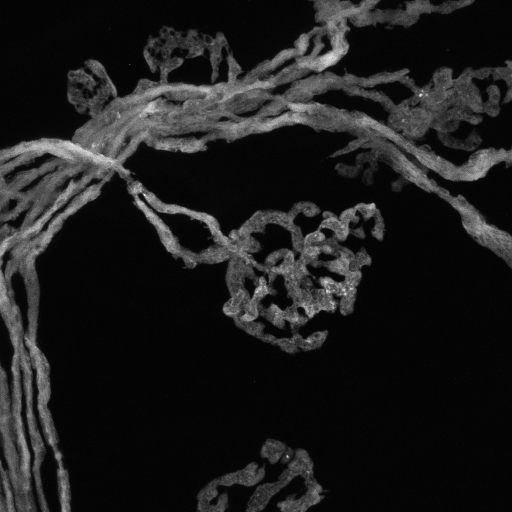
(a)

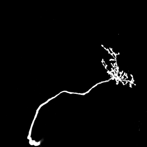
(b)

Figure 1: Images of two different neural structures obtained using confocal microscopy. The enormous variety of curvilinear structures requires problem-specific training datasets even in case of the same modality.

In this paper, we propose an Active Learning (AL) approach that exploits the specificities of delineation algorithms to massively reduce the effort and drudgery involved in collecting sufficient amounts of training data. At the heart of all AL methods is a query mechanism that enables the system to ask a user to label a few well chosen data samples, which it has selected based on how informative the answers are likely to be. AL has been successfully deployed in areas such as Natural Language Processing [26], Computer Vision [10], and Bioinformatics [15]. While it has made it possible to train classifiers with less of human intervention, none of the algorithms can exploit the fact that, for delineation purposes, the paths to be annotated form a graph in which neighborhood and geometric relationships can and should be considered.

In our approach, we explicitly use these relationships to derive multi-sample entropy estimates, which are better surrogates of informativeness than the entropy of individual samples that is typically used [12]. As a result, our queries focus more effectively on ambiguous regions in image space, that is, those at the boundary between positive and negative examples.

To avoid having to retrain the system after each individual query and further increase efficiency, we also integrate into our approach a batch strategy that lets the system ask the user several questions simultaneously. It incorporates density measures that ensure that the batches are diverse in features, representative of the delineation problem at hand and located near each other in the images so as to facilitate the interaction. This is particularly important in 3D volumes where scrolling from one region to another far away is cumbersome and potentially confusing for the user.

In short, our contribution is an AL approach that is tailored for the delineation of complex linear structures. In that sense, it is specialized. However, it is also generic in the sense that it can handle a wide variety of different structures. We will show that it outperforms more traditional approaches on both 2- and 3-D datasets representing different kinds of linear structures, that is, roads, blood vessels, and neural structures.

In the reminder of this paper, we first review existing AL techniques applicable to our problem and discuss their limitations for this purpose. We then introduce our approach and show how we combine information propagation and density measures to streamline the annotation process. Finally, we compare the performance of our approach against conventional techniques.

2 Related Work

AL is predicated on the idea that, given even very small amount of annotated data, the learning algorithm can actively choose additional instances that would be most profitable to label next. Starting from a small randomly chosen and manually annotated set of samples, iterating this process can drastically reduce the need for further human annotation since only the most informative ones are considered. This has been demonstrated in applications ranging from Natural Language Processing to Bioinformatics in which unlabeled data is readily available but annotation is expensive [23].

All such AL methods require a criterion for sample selection. The most popular one is uncertainty, usually defined as proximity to the classifier’s decision boundary. When the classifier is probabilistic, this can be evaluated in terms of entropy [24]. In practice, Uncertainty Sampling can be incorporated into most supervised learning methods such as SVMs [26], Boosting [8] and Neural Networks [4].

Another family of AL algorithms called query-by-committee [5] uses different automated “experts” to assign potentially different labels to each sample. Those for which the disagreement is the greatest are prime candidates for manual annotation.

Most practical AL algorithms allow the human to annotate batches of samples before retraining the classifier. This spares the need to wait for potentially lengthy computations to finish between each intervention. However, Uncertainty Sampling as described above can easily end up querying outliers and in batch mode - redundant instances, which is inefficient. This is usually addressed by considering not only the information gain potentially delivered by labelling each individual sample, but also the representativeness of each batch, which is accomplished by density-based methods. In [24], Settles and Carven introduce a information density-weighted framework, which favours samples that are not only uncertain but also representative of the underlying distribution. The main problem associated with this approach is finding the weighting of the two terms. Li and Guo [13] propose choosing a weight at each iteration that would minimise the future generalisation error. This approach is however computationally expensive, as it requires recomputing the underlying model many times and may additionally lead to overfitting.

Most of the methods discussed above originate from fields other than that of Computer Vision. They rarely exploit the contextual or spatial relations that are prevalent in images except for a few cases. In [25] contextual image properties are used to find the image regions that would convey the most information about other uncertain areas with which they are contextually related. In [17] a perplexity graph modelling similarities between images enables efficient hierarchical subquery evaluation. In video segmentation application [7], the obtained labels are propagated in a semi-supervised manner on a graph consisting of spatial, temporal and prior edges. Then, the most uncertain frame is selected for the next annotation. We will show that propagating information after preliminary classification and computing uncertainty only after this is advantageous over estimating informativeness based only on the result of classifier. The AL approach to segmenting CT scans of [9] incorporates context in terms of generative anatomy models. The notion of geometric uncertainty for segmentation is introduced in [11]. Like our algorithm, it relies on exchanging probability values between neighbours, but does not account for dataset diversity.

3 Active Learning for Delineation

Graph-based network reconstruction algorithms have recently shown superior performance compared to methods based on segmentation. They not only recover the geometry of the problem, but also the correct connectivity, which is crucial in applications such as neuroscience [21, 29, 18, 28, 27, 20]. They largely owe their performance to supervised Machine Learning techniques that allow them to recognize promising linear paths.

These methods usually start by computing a tubularity measure, which quantifies the likelihood that a tubular structure exists at given image location. Next, a set of subsampled high-tubularity superpixels [21, 29, 18] or longer paths [28, 27, 3, 20] are extracted. Each of them can be considered as an edge $e_{i}$ belonging to overcomplete spatial graph $\mathcal{G}$ and characterized by a feature vector $\mathbf{x}_{i}$. Given two possible class labels $\mathit{(y_{i}=1)}$ and $\mathit{(y_{i}=0)}$ , a discriminative classifier assigns to each edge $\mathit{e_{i}}$ probability of belonging to the structure of interest $\mathit{p(y_{i}=1|\mathbf{x}_{i})}$ or to the background, $\mathit{p(y_{i}=0|\mathbf{x}_{i})}$.

The optimal subgraph $\mathcal{T}^{*}$ can then be taken to be tree that minimizes the cost function over all trees $\mathcal{T}$ that are subgraphs of $\mathcal{G}$

$$\sum_{e_{i}\in E_{\mathcal{T}}}-\log\frac{p(y_{i}=1|\mathbf{x}_{i})}{p(y_{i}=0|\mathbf{x}_{i})},$$ (1)

where $E_{\mathcal{T}}$ represents the edges of $\mathcal{T}$. Provided that one does not take into account the geometry of the tree but only its topology, this can be shown to be Maximum a Posteriori estimate. In practice, however, it is more effective to formulate the MAP problem in terms of pairs of consecutive edges. This makes it possible to introduce better geometric constraints [28] and to find generic subgraphs as opposed to only trees [27].

Whether using single edges or pairs, the key requirement for this kind of approach to perform well is that the classifiers used to estimate the probabilities of Eq. 1 should be well-trained. This is especially important in ambiguous parts of the images such as those depicted by Fig. 2.

This necessitates significant amounts of ground-truth annotations to capture the large variability of the data and to cope with imaging artefacts and noise. To decrease the amounts of necessary time and effort, we introduce an AL algorithm that is suited to delineation problems represented on a graph. At each iteration it selects a sequence of consecutive edges from an overcomplete graph, such as the one described above, which should be labeled next in order to decrease the uncertainty in the most ambiguous image regions.

In theory the sequences could be of arbitrary length, that is 1,2, or more. In practice, we will see that 2 is near optimal because 2 consecutive edges are enough to capture some amount of geometry and because querying at each iteration more than 2 edges does not update the model frequently enough.

In the results section, we will use the algorithm of [27], which operates on edge pairs to produce the final delineations. However, our approach is generic and could be used in conjunction with any delineation pipeline that represents the problem on a graph and requires supervised edge classification.

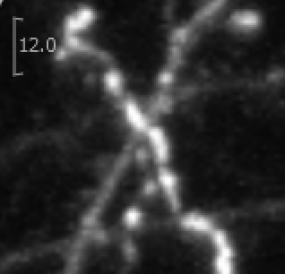
(a)

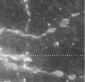
(b)

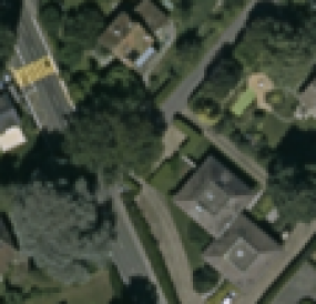
(c)

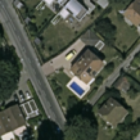
(d)

Figure 2: Ambiguous image regions. (a) Branch intersection. (b) Discontinuities due to uneven tissue staining. (c) Discontinuities due to occlusion by a tree. (d) Linear structures such as driveways that should be ignored.

4 Approach

In this section, we first cast the traditional Uncertainty Sampling approach into our chosen delineation framework. We then introduce our approach to probability propagation designed to rapidly identify ambiguous image regions and prevent the so-called sampling bias that may lead the classifier to explore irrelevant parts of the feature space. Finally, we combine this with an approach to batch density-based learning that simplifies the interaction while guaranteeing that the batches are representative and diverse enough to achieve rapid convergence.

4.1 Random and Uncertainty Sampling

The simplest strategy for picking samples to be annotated is to randomly choose them from a pool of unlabeled ones in so called Random Sampling (RS). As discussed in Section 2, Uncertainty Sampling (US) is a simple and popular approach to more efficient learning by querying first the most uncertain samples according to a metric, such as Shannon entropy.

In our case, as discussed in Section 3, each edge $e_{i}$ of the spatial graph $\mathcal{G}$ is assigned a feature vector $\mathbf{x}_{i}$ computed from the pixels surrounding the corresponding path. Let

$$p_{t}(y_{i}=y|\mathbf{x}_{i})\mbox{ for }y\in\{0,1\}$$ (2)

be the probabilities computed by classifier $C_{t}$ after $t$ AL iterations that $e_{i}$ lies on the centreline of a true structure or not. Let also $S_{t}$ be the set of $N_{t}$ annotated samples $(\mathbf{x}_{j},y_{j})_{1\leq j\leq N_{t}}$ used to train $C_{t}$. $p_{0}$ denotes the probabilities returned by the classifier using the small initial batch $S_{0}$ of annotated samples. When training is complete after $T$ iterations, $p_{T}$ is then used to compute the probabilities that appear in Eq. 1.

Given a classifier $C_{t-1}$ trained using the training set $S_{t-1}$, AL iteration $t$ involves choosing one or more unlabeled edges, asking the user to label them, adding them to the training set $S_{t-1}$ to form $S_{t}$ and, finally, training classifier $C_{t}$. In RS, this is done by randomly picking one or more $\mathbf{x}$ not already in $S_{t-1}$. In US, it is done by computing for each $\mathbf{x}$ the entropy:

$$H(\mathbf{x}) = -\log(p_{t-1}(y=0|\mathbf{x}))p_{t-1}(y=0|\mathbf{x})$$ (3)

$$-\log(p_{t-1}(y=1|\mathbf{x}))p_{t-1}(y=1|\mathbf{x})\;\;$$

and selecting the vector(s) with the highest entropy. Since $H(\mathbf{x})$ is largest when the classifier returns a $0.5$ value and minimum when it returns values close to zero or one, this assumes that those vectors whose probability of being a true path is computed to be $0.5$ are the most uncertain and closest to the decision boundary. Therefore annotating them is likely to help refine the shape of that boundary.

This approach can be effective but it can also fall victim to sampling bias. This happens when the current classifier is so inaccurate that its decision boundary is far away from the real one and the learner ends up focusing on an irrelevant part of the feature space. Our approach is designed to avoid this trap.

4.2 Probability Propagation

The probability $p_{t}$ returned by the path classifier takes into account the appearance of only a single path. By doing so, it neglects the information present in the wider neighborhood, provided by the other paths in the graph that share an endpoint with it. In particular, it ignores the fact that contiguous paths are more likely to share labels than non contiguous ones.

To account for this, we took inspiration from the semi-supervised learning method of [30] and implemented a modified version of it that propagates probabilities instead of labels. There, the label propagation is used to classify a large pool of unlabelled examples having only a few labelled instances. In our Probability Propagation Sampling (PPS) strategy we propagate the probabilities assigned by the base classifier to identify samples that differ significantly from their neighbourhood.

Let $\mathbf{P}_{0}$ be an $N\times 2$ matrix. Its entries are the probabilities $p_{t}(y_{i}=y|\mathbf{x}_{i})$ of Eq. 2 for all $N$ samples and $y\in\{0,1\}$, except for already annotated ones for which we clamp the values to zero or one depending on their label. The information is then propagated as follows:

1. Build an $N\times N$ affinity matrix $\mathbf{W}\in\mathbb{R}^{N\times N}$ with elements $w_{ij}=\exp(-||\mathbf{x_{i}}-\mathbf{x_{j}}||^{2}/2\sigma^{2})$ if $e_{i}$ and $e_{j}$ share a node and zero otherwise.

2. Build a symmetric matrix $\mathbf{S}=\mathbf{D}^{-1/2}\mathbf{W}\mathbf{D}^{-1/2}$, where $\mathbf{D}$ is diagonal with elements $d_{ii}~{}=~{}\sum_{j}w_{ij}$.

3. Iterate $\mathbf{P}^{i+1}=\alpha\mathbf{S}\mathbf{P}^{i}+(1-\alpha)\mathbf{P}_{0}$ followed by normalization of the rows of $\mathbf{P}^{i+1}$ until convergence, where $\alpha\in(0,1)$ specifies how much information is exchanged between neighbors and how much of the original information is retained. The series was shown to converge to $\mathbf{P}^{*}=(\mathbf{I}-\alpha\mathbf{S})^{-1}\mathbf{P}_{0}$ [30] and we will use the closed-form solution.

After the probability propagation, we can compute the entropy of each path at AL iteration t, but this time using the new estimates of probability $\mathit{p^{*}}$:

$$H(\mathbf{x}) = -\log(p^{*}_{t-1}(y=0|\mathbf{x}))p^{*}_{t-1}(y=0|\mathbf{x})$$ (4)

$$-\log(p^{*}_{t-1}(y=1|\mathbf{x}))p^{*}_{t-1}(y=1|\mathbf{x})\;\;$$

4.3 Density-based Batch Query

The scheme of Section 4.2 involves retraining the classifier each time the user has annotated a new sample, forcing them to wait for the computation to be over before intervening again. As discussed in Section 2, this is impractical and most practical AL approaches work in batch-mode, that is, they allow the user to annotate several samples before retraining.

In our case, samples are image paths and it is much easier to sample several paths in the same image region than over a wide space, which would imply scrolling through a potentially large 2D image or, worse, 3D image stack. Our solution to this is to present the annotator with consecutive paths represented by adjacent edges in the spatial graph $\mathcal{G}$ of Section 3. However, in order to be effective, individual paths should be:

1. informative to ensure that the new labels truly bring new information,

2. representative, that is, inliers of the statistical distribution of all samples,

3. diverse, that is, different from each other and from the already labeled ones.

The entropy measure of Eq. 4 can be used to assess the first of these three desirable properties. To measure the other two, we use the $N\times N$ affinity matrix $\mathbf{\widetilde{W}}$ obtained using the same parameters as the matrix $\mathbf{W}$ of Section 4.2, but whose elements are measures of pairwise similarity between each of the $N$ samples in the feature space, not only the neighbours in image.

Let $\mathit{L}$ be the indices of already labelled edges and $\mathit{E}_{k}$ be the set of all possible edge index combinations denoting $k$ consecutive paths. For each $E\in E_{k}$, we can compute the following similarity measures:

$$\sigma_{G}(E) = \sum_{i\in E}\sum_{1\leq j\leq N}w_{ij}$$ (5)

$$\sigma_{L}(E) = \sum_{i\in E}\sum_{l\in L}w_{il}$$ (6)

$$\sigma_{I}(E) = \sum_{i\in E}\sum_{j\in E,j\neq i}w_{ij},$$ (7)

where $\sigma_{G}(E)$ is a global similarity measure, $\sigma_{L}(E)$ measures similarity to already labelled samples and $\sigma_{I}(E)$ similarity within the batch. Intuitively, we want to maximize $\sigma_{G}$ to ensure representativeness and minimize $\sigma_{L}$ and $\sigma_{I}$ to improve diversity and explore the whole feature space. We therefore take

$$\mu(E)=\frac{\sigma_{G}(E)-\sigma_{L}(E)-\sigma_{I}(E)}{\sigma_{G}(E)},$$ (8)

to be our measure of both diversity and representativeness. This formulation does not require any additional parameters to weigh the effect of the three conditions or constructing any additional graphs in the feature space.

4.4 Combining Informativeness and Density Measure

PPS allows us for taking advantage of the current model while density-based query enables exploration of the feature space. In order to combine those two effects at each AL iteration we query the batch

$$E^{*}=\operatorname*{arg\,max}_{E\in\mathit{E}_{k}}\mu(E)(\sum_{i\in E}H(\mathbf{x}_{i}))\;$$ (9)

where $H$ is the entropy measure of Eq. 4 and $\mu(E)$ is calculated as in Eq. 8. In our Density-Probability Propagation Sampling (DPPS) the effects of exploration and exploitation are balanced during AL.

5 Results

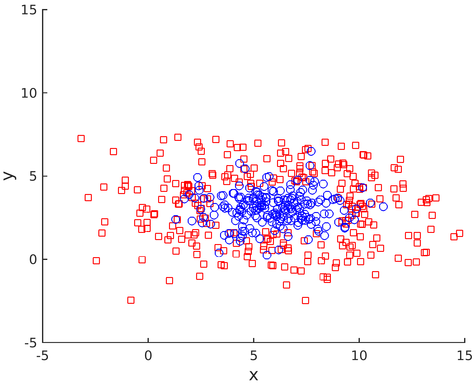
(a)

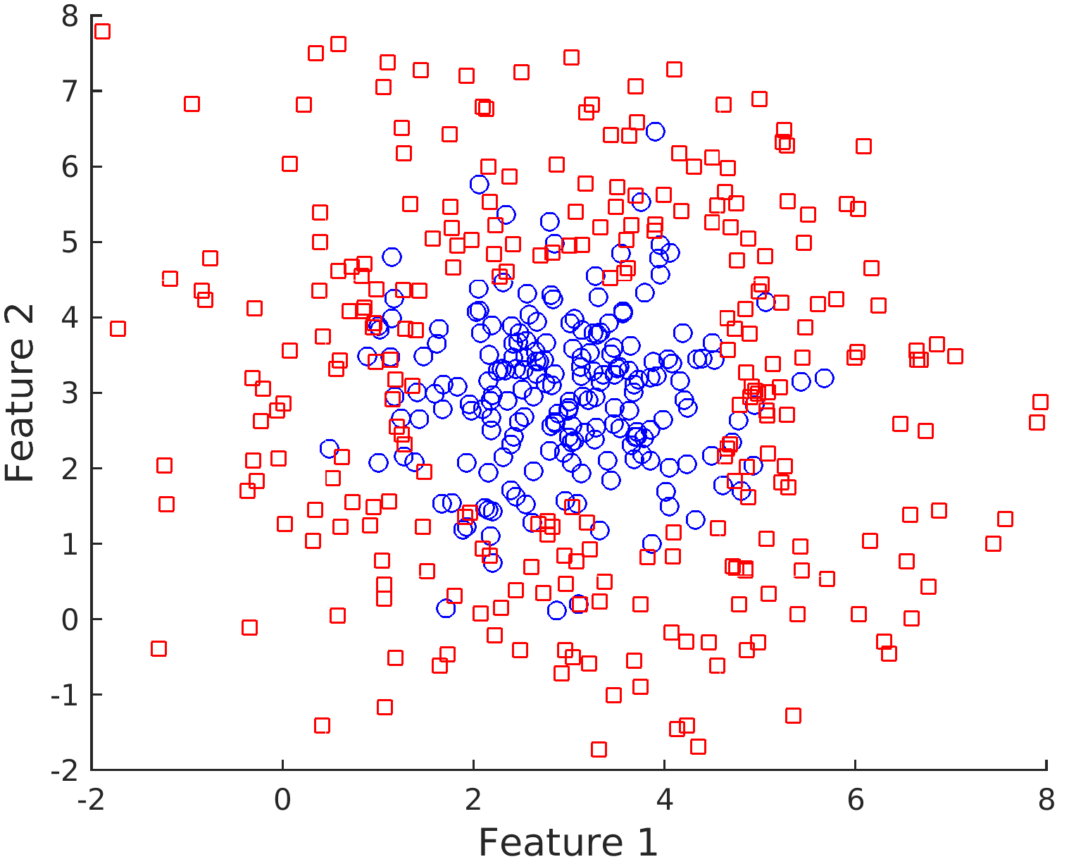
(b)

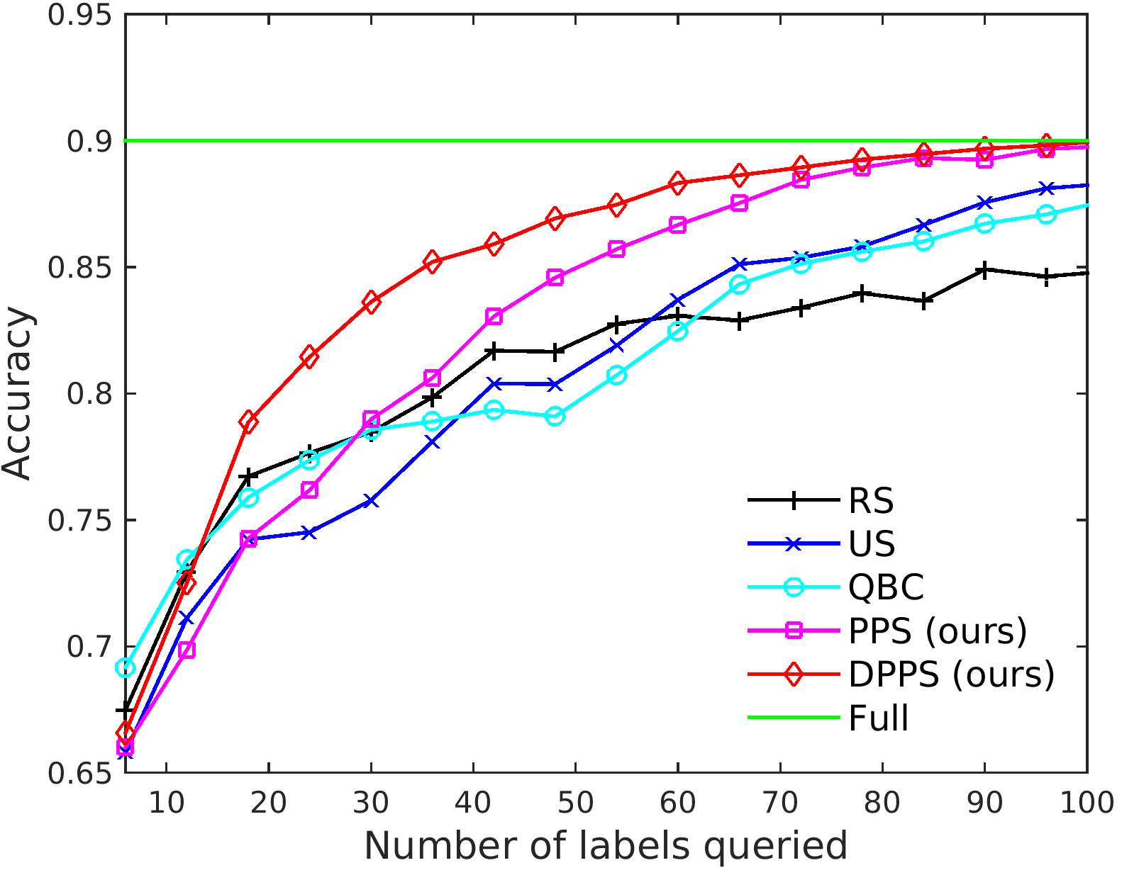
(c)

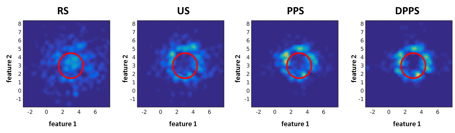
(d)

Figure 3: Synthetic dataset: (a) samples in the Euclidean space (b) samples in the feature space. (c) Classification results. (d) Query heat-maps in the feature space; the red circle indicates the optimal decision boundary. Best viewed in color.

In this section, we present our results; we first describe our experimental setup and baselines. We then introduce a synthetic dataset to help visualize the query decisions made by the different strategies. Finally, we show that our approach outperforms the conventional techniques on four real datasets.

5.1 Experimental Setup

We apply our AL approach for reconstruction of curvilinear networks in 2- and 3-D images. As discussed in Section 3, the overcomplete graphs, as well as the final delineations obtained once the classifiers have been properly trained are constructed using the delineation algorithm of [27]. The feature vectors associated to each path are based on Histogram of Oriented Gradients specially designed for linear structures. They capture the contrast, orientation, and symmetry of the paths.

The probabilities of Eq. 1 are computed by feeding the feature vectors to Gradient Boosted Decision Trees [2] with an exponential loss. We found it be well suited to interactive applications because it can be retrained fast, that is in under 3s for all the examples we show in this paper. To avoid overfitting especially in the initial stages of AL, we set the number of weak learners to 50, maximum tree depth to 2 and shrinkage to 0.06. Each tree is optimized using 50% of randomly selected data. Out of possible 303 features, 50 are investigated at each split. The classifier returns score F that can be then converted to probability using the logistic correction [19], that is,

$$p(y=1|x)=\frac{1}{1+\exp(-2F(x))}\;.$$ (10)

The edge connectivity matrix of Section 4.2 is computed on the basis of the overcomplete graphs.

The annotated ground truth data we have for all datasets, allows us to simulate the user intervention. We assume edges that are 10 pixels/voxels apart from the corresponding ground-truth path and with a normalised intersection exceeding 0.5 to be positive. We start each query by a random selection of 4 data points belonging to each class (background/network). Unless stated otherwise, we query 2 consecutive paths during each iteration and this choice is explained in Section 5.4. We proceed until the total number of labelled samples reaches 100. Each AL trial is repeated 30 times and the results are then averaged.

5.2 Baselines

We compare the two versions of our approach, Probability Propagation Sampling (PPS) and Density Probability Propagation Sampling (DPPS) as described in Sections 4.2 and 4.4, to the following baselines:

• Random Sampling (RS) - selecting a random pair at each iteration.

• Uncertainty Sampling (US) - selecting a pair with the highest sum of individual entropies as given by Eq. 3.

• Query-By-Committee (QBC) - selecting a pair that causes the greatest disagreement in a set of hypotheses, here represented by trees in a Random Forest. We measure the disagreement using the definition of [5].

For calibration purposes, we also report the classification performance using all the available training data at once (Full), that is, without any AL.

5.3 Synthetic Dataset

To compare the qualitative behavior of different strategies, we create a synthetic dataset. In the image space depicted by Fig. 3a, a positive class is surrounded by a negative one, which resembles what happens when trying to find real linear paths surrounded by spurious ones. We created feature space depicted by Fig. 3b by transforming the image coordinates and adding random noise so that the decision boundary in feature space does not correspond to the one in Euclidean space. We built the required spatial graph by connecting each point to its 10 nearest-neighbors in image space. We compute the weighting matrix $\mathbf{W}$ using RBF kernel with $\sigma$ = 1 and set probability propagation $\alpha$ to 0.9.

As can be seen in Fig. 3c, PPS and DPPS outperform the baselines and after querying 90 examples match the performance obtained by training on the whole training set. This corresponds to a 80% reduction in annotation effort. Furthermore, DPPS does better than PPS early on, Later in the process, once the most informative examples are all labeled, both approaches yield similar results.

In Fig. 3d, we use a heat map in feature space to depict the the most frequently queried regions and overlay the optimal decision boundary in red. They indicate that propagating information in a spatial graph helps refine the feature space faster than simple uncertainty query. Introducing density measures further constrains the search space making the process more effective and sampling more uniformly around the optimal decision boundary.

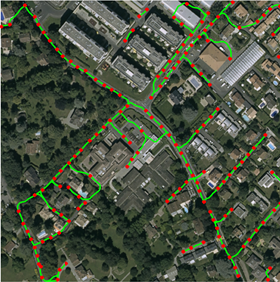
(a)

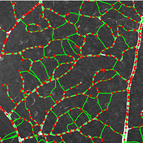
(b)

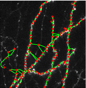
(c)

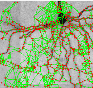
(d)

Figure 4: Training images with superimposed overcomplete graphs (a) Roads (b) Blood vessels (c) Axons (d) Brightfield neurons.

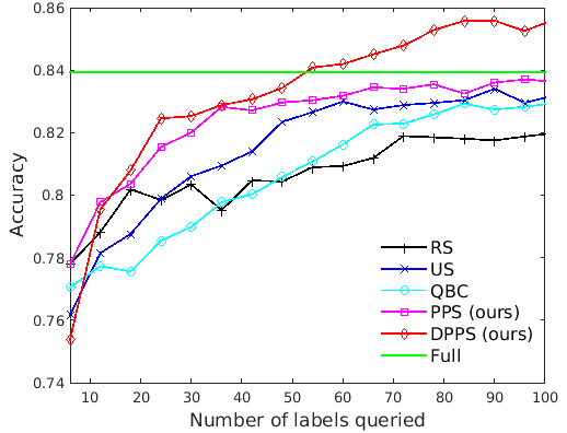
(a)

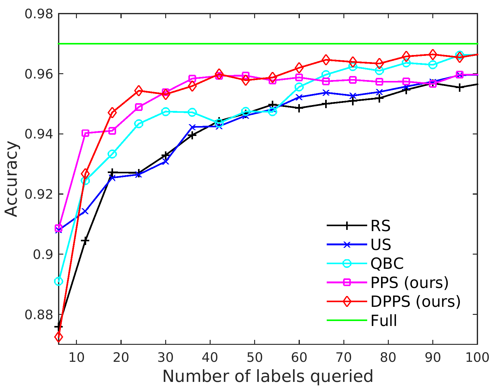
(b)

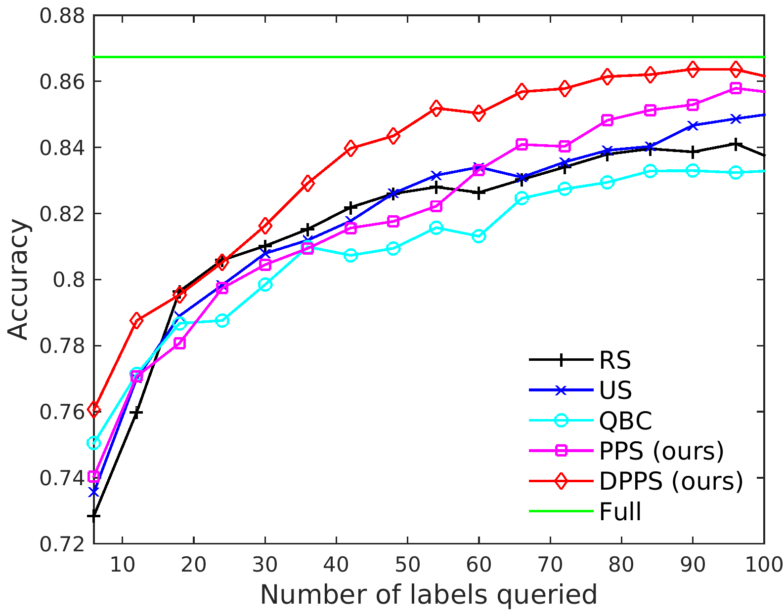
(c)

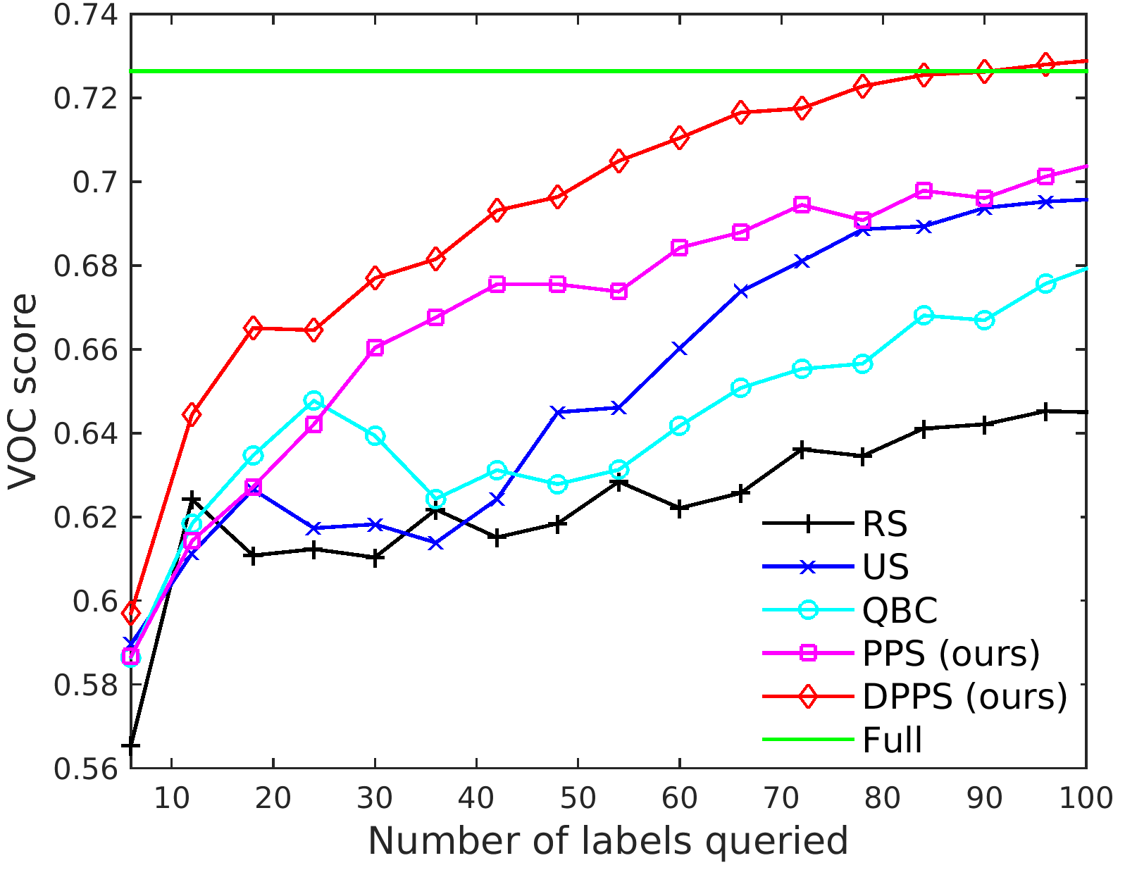
(d)

Figure 5: Classification results for the (a) Roads (b) Blood vessels (c) Axons (d) Brightfield neurons datasets.

5.4 Real Datasets

Roads

The dataset consists of 2D aerial images of roads. They include road patches occluded by trees and contain road-like structures such as driveways, thus making the classification task difficult.

We compute the weighting matrix $\mathbf{W}$ using RBF kernel with $\sigma$ = 1 and set probability propagation $\alpha$ to 0.9. As shown in Fig. 5a, both our approaches outperform the baselines and reach the full-dataset performance after as few as 50 samples, which corresponds to 75% reduction in annotation effort. Interestingly, the accuracy keeps increasing above the Full dataset accuracy. This behavior was already reported in [22] and suggests that in some cases a well chosen subset of data produces better generalization than the complete set. In Fig. 6 we present how the uncertainty about the training paths (as measured by Eq. 9) decreases as AL progresses. The analysis of the most frequently queried samples shown in Fig. 7a reveals that our method selects mainly the occluded paths and those at the intersections between two roads of different sizes or a road and a driveway. They correspond to the ambiguous cases discussed in Section 3 and presented in Fig. 2c and Fig. 2d. This makes it possible to learn the correct connectivity pattern and avoid mistakes as we postulated in Section 3. To verify this, we compare not only the classification performance, but also the quality of the final reconstruction. We run the full reconstruction framework with classification followed by an optimization step and evaluate the reconstruction using the DIADEM score [1]. It ranges from 0 to 1 with 1 being a perfect reconstruction. As shown in Fig. 7c, our approach outperforms the baselines also in terms of the quality of the final reconstruction. Interestingly, we again get a better result than by training with the Full dataset.

These results were obtained by querying pairs of edges. To test the influence of the length of the sequences we query, as discussed at the end of Section 3, we reran the experiments using singletons, pairs, and triplets. As can be seen in Fig. 8 and in the supplementary material for the other datasets, using pairs tends to give the best results and this is what we will do in the remainder of this paper. Note that we assume that annotating one edge counts as one label, but in reality the effort of annotating several consecutive edges is less than labeling the same number of instances at random locations, as the user does not need to scroll from one region to another.

Blood vessels

The image stacks depicting direction-selective retinal ganglion cells were acquired with confocal microscopes. They contain many cycles and branch crossings. We compute the weighting matrix $\mathbf{W}$ using RBF kernel with $\sigma$ = 0.7 and set $\alpha$ to 0.9. As shown in Fig. 5b, our two methods bring about considerable improvements, especially at the beginning of AL and in the second part perform similarly to QBC.

Axons

dataset consists of 3D 2-photon microscopy images of axons in a mouse brain. The main challenge associated with these images is low resolution in the z-dimension resulting in some disjoint branches being merged into one, which drastically changes the connectivity of the final solution.

We compute the weighting matrix $\mathbf{W}$ using RBF kernel with $\sigma$ = 3 and set $\alpha$ to 0.9. The accuracy plot (Fig. 5c) reveals that yet again our methods perform better than the baselines, especially in the later stages of learning, and result in a 65% reduction in the training effort. As seen in Fig 7b, the most frequently queried edges are concentrated in the regions where two branches seem to intersect in the xy-plane. In Fig. 7d we show that this again improves the quality of the final reconstruction.

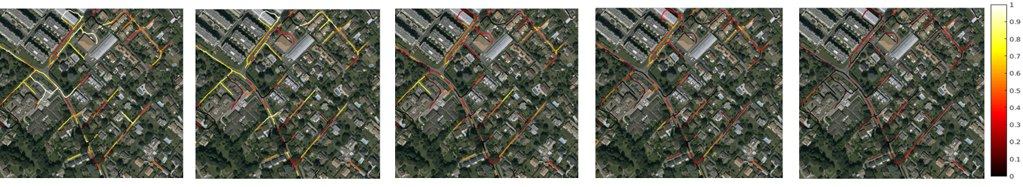
Figure 6: Color-coded ambiguity of the training paths given by Eq. 9 after 5, 15, 25, 35 and 45 AL iterations. The measure was normalized across the iterations. There is a clear decrease in the uncertainty as the learning progresses. Best viewed in color.

(a)

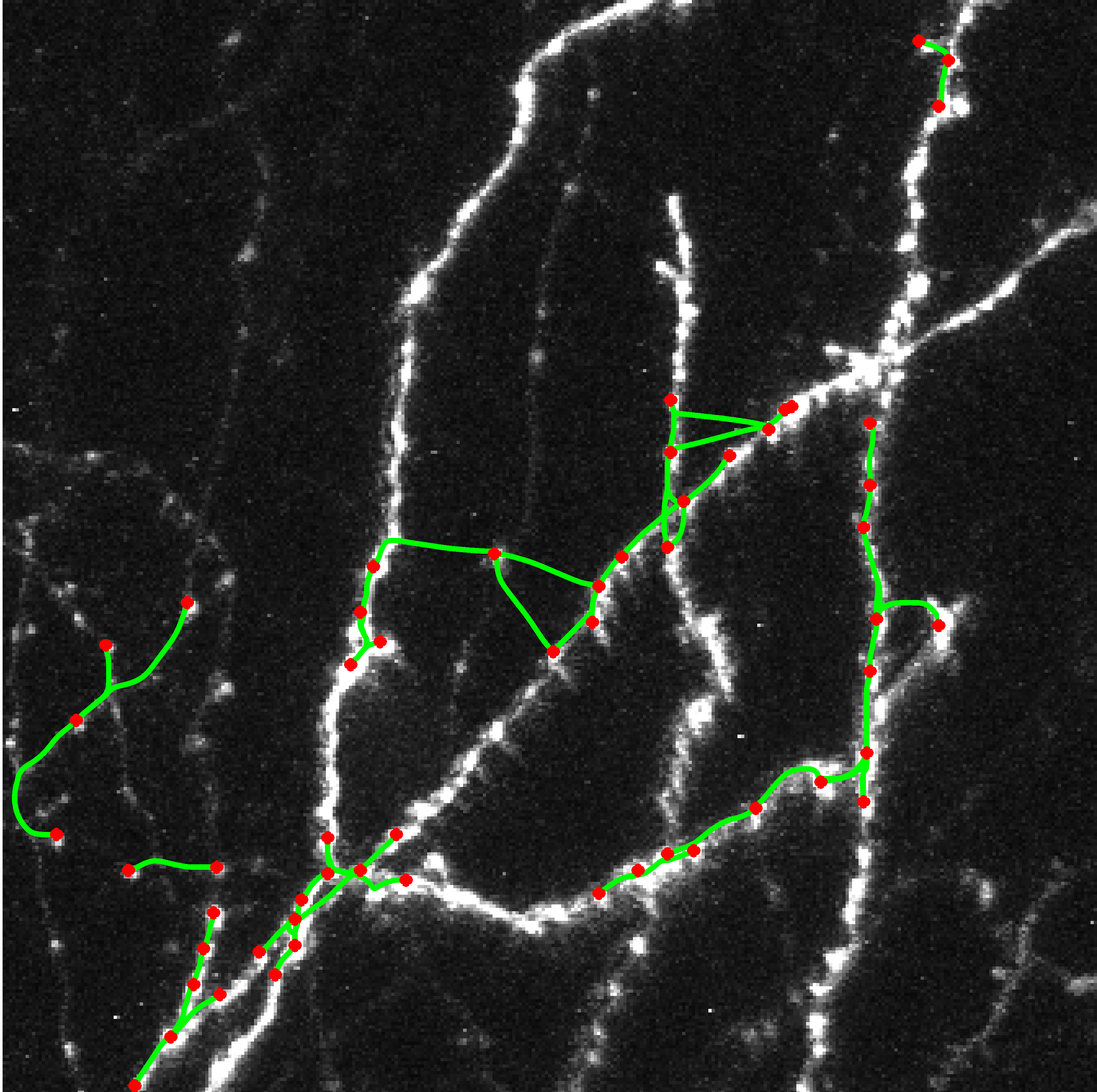
(b)

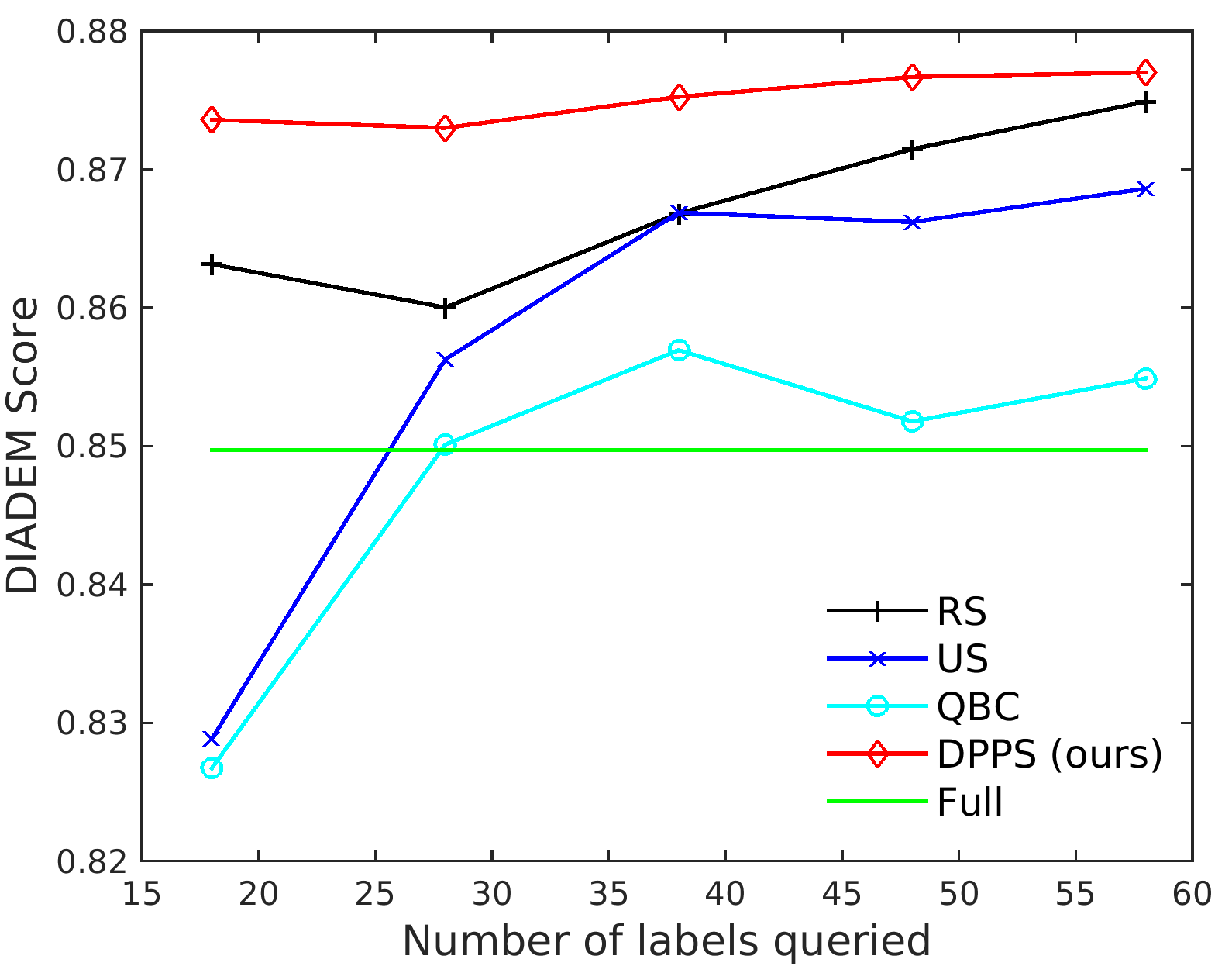
(c)

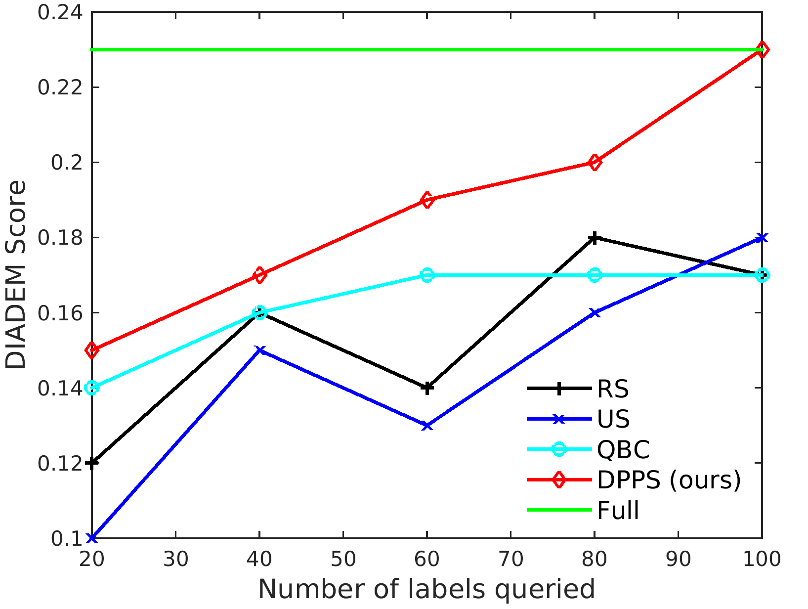
(d)

Figure 7: The most frequently queried samples for the (a) Roads and (b) Axons datasets. They often coincide with the ambiguous cases as discussed in Section 3. Averaged DIADEM scores of final reconstruction for the (c) Roads and (d) Axons datasets.

	RS	US	QBC	PPS	DPPS
Roads	0.00055	0.00040	0.00052	0.00036	0.00031
Blood vessels	0.00052	0.00071	0.00028	0.00019	0.00019
BF neurons	0.0040	0.0017	0.0008	0.0007	0.0003
Axons	0.00060	0.00061	0.00047	0.00048	0.00043

Table 1: Variance of the results.

Brightfield neurons

The dataset consists of 3D images of neurons from biocytin-stained rat brains acquired using brightfield microscopy. As in the Axons dataset, the z-resolution is low. The corresponding training graph is much bigger than in the previous 2 cases and consists of more than 3000 edges, most of which are negative. To assess the performance of different methods, we compute the VOC score [6] instead of accuracy. This is due to the fact that in this dataset around 95% of the edges are negative and the VOC score does not take into account true negatives. We compute the weighting matrix $\mathbf{W}$ using RBF kernel with $\sigma$ = 1 and set $\alpha$ to 0.9. As seen in Fig. 5d, our methods outperform RS, US and QBC. For US and QBC, we can notice the possible effects of bias trap, when the performance does not change for a few iterations, even though more and more labels are queried.

Note that each of the experiments was repeated 30 times and the results are averaged. In Table 1 we present also the variance of the results. In all cases except for one PPS approach shows smaller variance than the baselines and DPPS yields even lower variance.

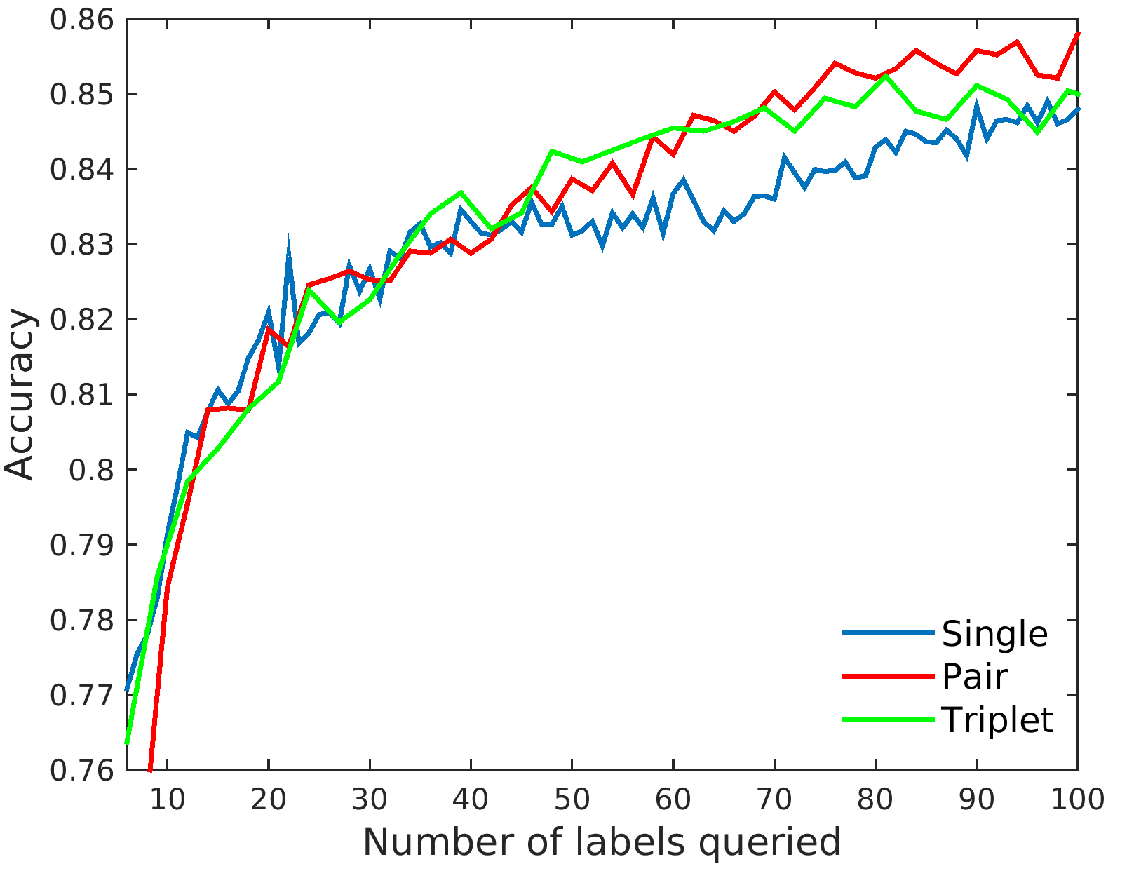
Figure 8: The classification performance for different batch sizes for the Roads dataset.

6 Conclusion

In this paper we introduced an approach to incorporating the geometrical information that increases the effectiveness of AL for the delineation of curvilinear networks. Additionally, we introduced a density-based strategy, which ensures that the selected batches are informative, diverse and representative of the underlying distribution. It also allows us to query sequences of consecutive paths, further reducing the annotation effort. Our approach showed superior performance for a wide range of networks and imaging modalities when compared to a number of conventional methods.

References

- [1] G. Ascoli, K. Svoboda, and Y. Liu. Digital Reconstruction of Axonal and Dendritic Morphology DIADEM Challenge, 2010.
- [2] C. Becker, R. Rigamonti, V. Lepetit, and P. Fua. Supervised Feature Learning for Curvilinear Structure Segmentation. In Conference on Medical Image Computing and Computer Assisted Intervention, September 2013.
- [3] D. Breitenreicher, M. Sofka, S. Britzen, and S. Zhou. Hierarchical Discriminative Framework for Detecting Tubular Structures in 3D Images. In International Conference on Information Processing in Medical Imaging, 2013.
- [4] D. Cohn, Z. Ghahramani, and M. Jordan. Active Learning with Statistical Models. Journal of Artificial Intelligence Research, 1996.
- [5] I. Dagan and S. P. Engelson. Committee-Based Sampling For Training Probabilistic Classifiers. In Proceedings of the Twelfth International Conference on Machine Learning, 1995.
- [6] M. Everingham, C. W. L. Van Gool and, J. Winn, and A. Zisserman. The Pascal Visual Object Classes Challenge (VOC2010) Results, 2010.
- [7] A. Fathi, M. Balcan, X. Ren, and J. Rehg. Combining Self Training and Active Learning for Video Segmentation. In BMVC, 2011.
- [8] J. Huang, S. Erekia, Y. Song, H. Zha, and C. Giles. Efficient Multiclass Boosting Classification with Active Learning. In SIAM International Conference, 2007.
- [9] J. Iglesias, E. Konukoglu, A. Montillo, Z. Tu, and A. Criminisi. Combining Generative and Discriminative Models for Semantic Segmentation. In Information Processing in Medical Imaging, 2011.
- [10] A. Kapoor, K. Grauman, R. Urtasun, and T. Darrell. Active Learning with Gaussian Processes for Object Categorization. In International Conference on Computer Vision, 2007.
- [11] K. Konyushkova, R. Sznitman, and P. Fua. Introducing Geometry into Active Learning for Image Segmentation. In International Conference on Computer Vision, 2015.
- [12] D. Lewis and W. Gale. A Sequential Algorithm for Training Text Classifiers. In ACM SIGIR proceedings on Research and Development in Information Retrieval, 1994.
- [13] X. Li and Y. Guo. Adaptive Active Learning for Image Classification. In CVPR, 2013.
- [14] T.-Y. Lin, M. Maire, S. Belongie, J. Hays, P. Perona, D. Ramanan, P. Dollár, and C. Zitnick. Microsoft COCO: Common Objects in Context. In European Conference on Computer Vision, pages 740–755, 2014.
- [15] Y. Liu. Active learning with support vector machine applied to gene expression data for cancer classification. J. Chemistry Information and Computer Science, 2004.
- [16] C. Long, G. Hua, and A. Kapoor. Active Visual Recognition with Expertise Estimation in Crowdsourcing. In International Conference on Computer Vision, 2013.
- [17] O. Mac Aodha, N. Campbell, J. Kautz, and G. Brostow. Hierarchical Subquery Evaluation for Active Learning on a Graph. In CVPR, 2014.
- [18] J. Montoya-Zegarra, J. Wegner, L. Ladicky, and K. Schindler. Mind the Gap: Modeling Local and Global Context in (Road) Networks. In German Conference on Pattern Recognition, 2014.
- [19] A. Niculescu-Mizil and R. Caruana. Obtaining Calibrated Probabilities from Boosting. In Conference on Uncertainty in Artificial Intelligence, 2005.
- [20] P.Neher, M.Götz, T.Norajitra, C.Weber, and K.Maier-Hein. A Machine Learning Based Approach to Fiber Tractography Using Classifier Voting. In Medical Image Computing and Computer-Assisted Intervention. 2015.
- [21] A. Santamaría-Pang, P. Hernandez-Herrera, M. Papadakis, P. Saggau, and I. A. Kakadiaris. Automatic Morphological Reconstruction of Neurons from Multiphoton and Confocal Microscopy Images Using 3D Tubular Models. Neuroinformatics, 2015.
- [22] G. Schohn and D. Cohn. Less is More: Active Learning with Support Vector Machines. In International Conference on Machine Learning, 2000.
- [23] B. Settles. From Theories to Queries : Active Learning in Practice. Active Learning and Experimental Design, 2011.
- [24] B. Settles and M. Craven. An analysis of active learning strategies for sequence labeling tasks. In Conference on Empirical Methods in Natural Language Processing, 2008.
- [25] B. Siddiquie and A. Gupta. Beyond active noun tagging: Modeling contextual interactions for multi-class active learning. In CVPR, 2010.
- [26] S. Tong and D. Koller. Support Vector Machine Active Learning with Applications to Text Classification. Machine Learning, 2002.
- [27] E. Turetken, F. Benmansour, B. Andres, H. Pfister, and P. Fua. Reconstructing Loopy Curvilinear Structures Using Integer Programming. In Conference on Computer Vision and Pattern Recognition, June 2013.
- [28] E. Turetken, F. Benmansour, and P. Fua. Automated Reconstruction of Tree Structures Using Path Classifiers and Mixed Integer Programming. In Conference on Computer Vision and Pattern Recognition, June 2012.
- [29] J. Wegner, J. Montoya-Zegarra, and K. Schindler. Road Networks as Collections of Minimum Cost Paths. International Society for Photogrammetry and Remote Sensing, 108:128–137, 2015.
- [30] D. Zhou, O. Bousquet, T. N. Lal, J. Weston, and B. Scholkopf. Learning with Local and Global Consistency. In NIPS, 2004.