Disk Emission from Magneto-hydrodynamic Simulations of Spinning Black Holes

Abstract

We present the results of a new series of global 3D relativistic magneto-hydrodynamic (MHD) simulations of thin accretion disks around spinning black holes. The disks have aspect ratios of $H/R\sim 0.05$ and spin parameters $a/M=0,0.5,0.9$, and $0.99$. Using the ray-tracing code Pandurata, we generate broad-band thermal spectra and polarization signatures from the MHD simulations. We find that the simulated spectra can be well fit with a simple, universal emissivity profile that better reproduces the behavior of the emission from the inner disk, compared to traditional analyses carried out using a Novikov-Thorne thin disk model. Lastly, we show how spectropolarization observations can be used to convincingly break the spin-inclination degeneracy well-known to the continuum fitting method of measuring black hole spin.

1 Introduction

Recent years have seen great strides in our ability to simulate global properties of accretion disks in a fashion dependent on actual physical mechanisms rather than ad hoc phenomenological models. Beginning a decade ago, several algorithms have been developed capable of treating 3D MHD in full general relativity (De Villiers & Hawley, 2003; Gammie et al., 2003; Noble et al., 2009; Penna et al., 2010). With those algorithms, it has become possible to study the bolometric energy budget of radiatively efficient accretion onto black holes (Noble et al., 2009; Penna et al., 2010; Avara et al., 2015), and from it predict details of the spectra of stellar-mass black holes both in the thermal-dominant state (Noble et al., 2011; Kulkarni et al., 2011; Zhu, 2012) and in other spectral states (Schnittman et al., 2013). Potentially, fits of these predictions to measured spectra taken in the thermal state could be used to constrain the spin of the black hole and the inclination of the disk (Davis et al., 2011; Gou et al., 2011; Steiner et al., 2011; Gou et al., 2014).

However, to make these measurements quantitative requires careful attention to a variety of sources of systematic error. Possible contributors to the error budget include uncertainties about atmospheric effects, both LTE and non-LTE, the disk inclination angle (spectral fitting leaves spin and inclination degenerate), the vertical structure of disks, and the intrinsic surface brightness profile of the disk. The two latter issues are both amenable to study through simulations, but both also exhibit subtle sensitivities to algorithm (e.g., the consequences of internal radiation pressure: Hirose et al. (2009); Jiang et al. (2013)) and grid resolution. In particular, after the first generation of global energy budget simulations were completed, Hawley et al. (2011) showed that only one of them (ThinHR: Noble et al. (2010)) even came close to having the spatial resolution required for a proper description of nonlinear MHD turbulence in the disk context; the others all fell far short. Unfortunately, the Noble et al. work treated only a Schwarzschild spacetime and therefore gave little aid to constraining spin.

It is the first goal of this paper to present three new simulations in Kerr spacetime (spin parameters $a/M=0.5$, 0.9, and 0.99) with resolution and vertical scale height comparable to that of the Noble et al. Schwarzschild simulation. With the resulting data, we have constructed predictions of the surface brightness profile and the resulting thermal spectra and compare them to previous results. Additionally, we make predictions of spin-dependent effects in the polarization spectrum of the thermal state, and show how spectropolarization observations can break degeneracies that have traditionally plagued the continuum fitting method for measuring spin. Lastly, we present a new analytic model for the emissivity profile of disks in the thermal-dominant state, applicable to any value of $a/M$.

In general, we find these new simulations lead to results similar to the non-spinning case described in Noble et al. (2011). Namely, the MHD disks produce a significant amount of additional flux in the region around the inner-most stable circular orbit (ISCO). This additional luminosity is manifest in a small, but consistent, increase in flux at the high-energy tail of the thermal spectrum as measured by a distant observer. Fitting the simulated spectra to traditional analytic thin disk models (e.g., Novikov & Thorne (1973)) therefore leads to small but significant bias towards higher spin parameters. Our proposed emissivity profile provides a better overall fit to the data, as well as generally a more faithful inference of the spin parameter.

2 Simulation Data

2.1 Global fluid properties

Our simulations were carried out with the Harm3d code (Noble et al., 2009) and were designed to resemble closely the ThinHR Schwarzschild simulation of Noble et al. (2010). All used the same cooling function and target temperature profile, designed to keep the disk aspect ratio $H/r\simeq 0.05$. All also began with the same initial condition, a hydrostatic torus with a pressure maximum at $r=35M$ and an inner edge at $r=20M$ (here and subsequently, we use units in which $G=c=1$). Threading these tori there was a dipolar magnetic field with mean initial plasma $\beta=100$. The spatial grids for the three Kerr spacetime simulations were very similar to the one utilized for the Schwarzschild case; the only alteration was to extend the radial grid to smaller Kerr-Schild radii in order to follow the shrinkage of the event horizon with increasing spin. As in the earlier work, our radial grid was logarithmic (i.e., constant $\Delta r/r\simeq 0.004$) and stretched from just inside (5 cells) the event horizon to $r=70M$. Consequently, there were 912, 960, 1020, and 1056 radial cells in the simulations with $a/M=0$, 0.5, 0.9, and 0.99, respectively. In all four simulations, there were 160 cells in the polar angle direction, and these cells were strongly concentrated to the equatorial plane. Likewise in all cases, the simulation domain included only the 1/4 circle from $\phi=0$ to $\phi=\pi/2$, with 64 cells across that range and periodic boundary conditions that mapped cells at $\phi=0$ to $\phi=\pi/2$. Boundary conditions on the inner and outer radial surfaces were outflow; the polar-angle boundaries at the axis ($\theta=0,\pi$) were continuous across the pole.

The ThinHR simulation was run to a time 15,000$M$; the Kerr simulations were run to $\simeq$17,000 – 18,000$M$. As is generally the case, inflow equilibrium, to the degree it is achieved, begins at the ISCO and gradually moves outward. It can be characterized in (at least) two ways: by a statistical steady-state in the accretion rate onto the black hole and by constancy in the accretion rate as a function of radius when time-averaged over the period of interest. Here we show both measures.

Figure 1 shows how the accretion rate through the event horizon varied over time in all four simulations. The peak accretion rates were similar in all four simulations, but, particularly at late times, there is a tendency for the accretion rate to diminish with increasing spin. This tendency was also seen in earlier global simulations with thicker disks and shorter durations (Krolik et al., 2005). Because the period before 10,000$M$ tends to be dominated by transients associated with initial channel solutions, we have restricted our analysis of disk output to periods after that time, 10,000 – 15,000$M$ for $a/M=0$, 0.5, and 0.9, 12,000 – 15,000$M$ for $a/M=0.99$.

Figure 1: Accretion rate as a function of time for all four simulations; from left to right and then top to bottom, they are $a/M=0.0$, 0.5, 0.9, and 0.99. The units of accretion are fractions of the initial mass on the grid per $M$.

Despite large variations in the time-dependent accretion rate at the horizon, the time-averaged accretion rate had relatively little variation in radius, a sign that overall there was little change in the disk’s mass distribution. To illustrate that fact, in Figure 2 we show the ratio $\langle\dot{M}(r)\rangle/\langle\dot{M}(r_{H})\rangle$ as a function of $r/r_{\rm ISCO}$. Both axes are logarithmic in order to emphasize that ratios are what matter most in this context. Inflow equilibrium is best judged in terms of fractional departures in the accretion rate; radial variation is best considered in units of $r_{\rm ISCO}$ because the greatest energy release takes place at or near the ISCO and, in the Newtonian limit, the potential is a power-law in radius. In three of the four cases ($a/M=0$, 0.9, and 0.99), the time-averaged accretion rate changes by at most a few tens of percent for $r\lesssim 3r_{\rm ISCO}$. In the case of $a/M=0.5$, this criterion is achieved only out to $r\simeq 2r_{\rm ISCO}$, beyond which it rises to about twice the accretion rate at the horizon.

Figure 2: Time-averaged accretion rate as a function of radius in ratio to the rate at the horizon for all four simulations; from left to right and then top to bottom, they are $a/M=0.0$, 0.5, 0.9, and 0.99. The unit of radius in each case is the radial coordinate of the ISCO for that spin.

Over these time periods, the MRI quality factors for all four simulations were quite good. We measured the quality factors $Q_{z}$ (the mean number of cells per fastest growing vertical wavelength) and $Q_{\phi}$ (the mean number of cells per fastest growing toroidal azimuthal wavelength) by constructing mass-weighted averages on spherical shells and then time-averaging over the same periods for which inflow equilibrium was evaluated (Noble et al., 2010; Hawley et al., 2011). When $a/M=0$, $Q_{z}\simeq 25$ and $15\lesssim Q_{\phi}\lesssim 20$ across the entire range of radii; when $a/M=0.5$, $15\lesssim Q_{z}\lesssim 30$ and $10\lesssim Q_{\phi}\lesssim 25$, with comparable quality factors for $a/M=0.9$ and $a/M=0.99$. These numbers compare very favorably with the standard set by Hawley et al. (2011) and Sorathia (2012) that for proper description of the nonlinear development of MHD turbulence in accretion disks if $Q_{\phi}\gtrsim 20$, then $Q_{z}$ should be $\gtrsim 10$.

2.2 Radiation

Given the density, cooling rate, and four-velocity of the fluid at each point in the simulation, we construct a disk surface temperature map as in Noble et al. (2011). For the purpose of ray-tracing to infinity, we remove the geometric effects of finite disk thickness, assuming that all the thermal flux comes from a thin disk near the midplane, while still preserving the time and azimuthal variability in the simulation data. Kulkarni et al. (2011) do the former, but not the latter, leading to systematically softer spectra. The radiation is emitted from this surface with the limb-darkening and polarization properties appropriate for a scattering-dominated, optically thick atmosphere (Chandrasekhar, 1960).

Since we are in this paper primarily focused on the thermal state, in which the coronal Compton-$y$ parameter is expected to be small, we ignore any scattering in the corona (to a large degree, in the thermal state, the corona can simply be thought of as an extension of the accretion disk atmosphere). The photons therefore follow geodesic paths from the disk until they reach the distant observer or are captured by the event horizon. However, because we are also interested in polarization signatures, we include scattering of returning radiation off the optically-thick disk body, as in Schnittman & Krolik (2009).

As a test of this method, we have also tried using emission models that include only the disk proper, as defined by the region between electron-scattering photospheres, as in Schnittman et al. (2013). This approach requires specifying a physical accretion rate in order to fix the density scale in cgs units. For $\dot{m}=0.03$ in Eddington units (roughly the lower limit of the thermal-dominant state), we find that, for the $a/M=0$ run, roughly $80\%$ of the dissipation takes place in the disk proper, with that number rising to $90\%$ for the spinning cases. For all cases, we find that the coronal and disk radial emissivity profiles are nearly identical. Thus, if we were to include only the disk emission, the thermal luminosity would decrease slightly, but the spectral shape remains unchanged.

3 Results

3.1 Efficiency

One of the most basic results that comes from these global MHD simulations is the total radiative efficiency of the thin accretion disk. Astrophysically, this number is critical for connecting the accretion history and growth of super-massive black holes in the universe with the observed luminosity and mass distribution functions (Soltan, 1982). While it is almost impossible to measure the efficiency of an individual black hole, the shape of the thermal spectrum (which of course is observable) is empirically related to the radiative efficiency because higher efficiency is typically due to higher emission at small radii, producing higher temperatures and harder spectra.

In Table 1 we show several measures of the radiative efficiency. We define $\eta$ (radiated) to be the ratio between the time-averaged luminosity emitted by the disk and the time-averaged rest-mass accretion rate (photon energy and observer time both measured at infinity). Similarly, $\eta$ (captured) is the ratio of the time-averaged luminosity crossing the horizon to the time-averaged accretion rate (for photons crossing the horizon, the energy-at-infinity is easy to measure: $E_{\infty}=-p_{t}$). Thus the net radiative efficiency measured at infinity is $\eta$(radiated)-$\eta$(captured).

$\eta_{\rm NT}$ is the classical Novikov-Thorne efficiency, and $\eta_{\rm Harm3d}$ is calculated from our simulations. Note that $\eta_{\rm NT}$ (radiated) is identical to the specific binding energy of a test particle orbiting at the ISCO. Lastly, for the simulation data, we also show $\eta_{\rm Harm3d}$ (advected), a measure of the accreted energy carried into the hole in the form of heat and magnetic field. In principle, this energy could be liberated via additional radiation mechanisms.

As first shown in Thorne (1974), we find that very little radiation is actually captured by the black hole. Although the additional flux emitted near and inside the ISCO leads to somewhat higher capture fractions than the NT model would predict, it is still less than $5\%$ of the total emitted flux even for $a/M=0.99$. In the end, the net radiative efficiency is quite close to $\eta_{\rm NT}$, as the additional MHD dissipation is negated by capture and advection, consistent with earlier work (Noble et al., 2011; Kulkarni et al., 2011). As shown in Noble et al. (2011), much of the increase in radiative efficiency relative to NT is due to the enhanced emission near the ISCO, both immediately inside and outside that radius.

In a certain sense, our figures for the efficiency are conservative estimates. By adopting an initial condition with nested dipolar field loops, we assure that there is some net magnetic flux trapped on the event horizon, but in terms of the $\Upsilon$ measure introduced by Gammie (1999), it is smaller than the maximum that can be achieved. Here we use the definition of McKinney et al. (2012), in which $\Upsilon\equiv 0.2\Phi/(r_{g}\sqrt{\dot{M}c})$, for accretion rate $\dot{M}$, gravitational radius $r_{g}$, and $\Phi$ the integral of the absolute value of the radial magnetic field around a spherical surface containing the black hole.

When $\Upsilon\simeq 6$ (roughly $3\times$ the value in our simulation), Avara et al. (2015) found that the radiative efficiency of a disk with somewhat greater aspect ratio ($h/r\simeq 0.1$) orbiting in an $a/M=0.5$ spacetime was roughly double what we found for the same spin parameter. This contrast suggests that the magnetic augmentation to radiative efficiency rises very sharply over the range in $\Upsilon$ between these values. However, in thermal states of black hole binaries, which do not show evidence of radio jets, one might not expect such large values of $\Upsilon$. Moreover, the intrinsic field topology in accreting black holes is entirely unknown. Other sorts of field topology—higher-order multipoles in the poloidal field or intrinsically toroidal field—may exist, and how the efficiency behaves as a function of net toroidal flux, etc., remains to be explored. All that can be said at the moment is that for $\Upsilon$ comparable to or smaller than in our simulations, the internal magnetic stresses depend only weakly on the field topology (Beckwith et al., 2008).

We see significant variability of the accretion rate and radiative efficiency within each simulation, as well as qualitative differences from one simulation to the next (e.g., differences in the radial fluid properties that do not appear to vary monotonically with spin), representative of the stochastic nature of the turbulent MHD disks. In principle, we could carry out an ensemble of runs for each spin to measure both the mean radiative efficiency and the variance of the observed efficiency due to the random fluctuations in the simulations. However, even the four simulations we did carry out were extremely expensive computationally, and any more would be very difficult to justify.

Table 1: For a range of spins, the emitted bolometric radiative efficiency $\eta$ (radiated) and the fraction of flux captured by the black hole $\eta$ (captured), for both NT disks and Harm3d simulations. Also listed is the fraction of advected thermal and magnetic energy in the MHD simulations.

$a/M$	$\eta_{\rm NT}$	$\eta_{\rm NT}$	$\eta_{\rm Harm3d}$	$\eta_{\rm Harm3d}$	$\eta_{\rm Harm3d}$
	(radiated)	(captured)	(radiated)	(captured)	(advected)
0.0	0.0572	0.0001	0.0607	0.0020	0.0080
0.5	0.0821	0.0005	0.0833	0.0016	0.0120
0.9	0.1558	0.0027	0.1600	0.0048	0.0115
0.99	0.2640	0.0087	0.2461	0.0111	0.0220

3.2 Radial luminosity profile

In Figure 3 we plot the radial luminosity profile $dL/dr$ for each of the black hole spins. In each plot, the solid red curve represents the time- and angle-averaged emitted flux from the Harm3d simulation data. The red dashed curve is the flux that reaches infinity, and the red dotted curve is the flux captured by the black hole. The solid black curve is the emitted flux from an NT disk.

All four cases share a number of qualitative features. The emission per unit radial coordinate peaks a short distance outside the ISCO, then decreases slightly before leveling off in the plunging region. Inside a point roughly halfway between the ISCO and the horizon, the flux emitted by the inward-flowing gas is almost entirely captured by the black hole. Contrasts also exist. For example, compared to the others, the fraction of the luminosity emitted in the $a/M=0.5$ plunging region is relatively small. The fluctuations alluded to earlier are large enough that these contrasts may be due to our comparatively short averaging times.

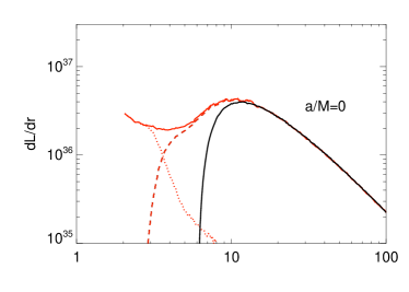
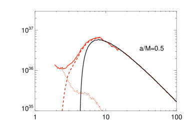
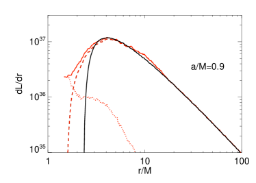
Figure 3: Luminosity profile $dL/dr$, integrated over $\theta$ and $\phi$, and averaging over time. The solid red curve is the Harm3d emission, the dashed curve is the flux reaching infinity, and the dotted curve is the flux captured by the black hole. The solid black curve corresponds to the Novikov-Thorne prediction for emission. For all cases, the Eddington-normalized accretion rate is $\dot{m}=0.1$.

Because the ISCO position in Boyer-Lindquist coordinates is a function of spin, detailed comparison of the four cases’ radial profiles requires defining a new radial coordinate relative to which the emission profiles are the most similar. Beckwith et al. (2008) found that simply scaling the radial coordinate by $r_{\rm ISCO}$, i.e., using $r^{\prime}\equiv r/r_{\rm ISCO}$, gives a roughly universal emissivity profile for NT disks, but not MHD disks. To unite MHD disks around black holes of different spins, we have instead developed a coordinate transformation based on the differential proper radial distance $d\tilde{r}=g_{rr}^{1/2}dr$. This coordinate transformation requires a constant of integration, or alternatively a free parameter that allows us to choose the radius at which $\tilde{r}=r$. We do this at $r=\frac{3}{2}r_{\rm ISCO}$, corresponding closely to the radius of peak emissivity. Finally, we scale by $r_{\rm ISCO}$ to make the radial coordinate dimensionless: $r^{\ast}\equiv\tilde{r}/r_{\rm ISCO}$. Note that in these coordinates, the horizon is located at negative $r^{\ast}$, but the vast majority of the flux is emitted outside of $r^{\ast}=0$, where the Boyer-Lindquist radial coordinate is $r\approx 1.15r_{\rm hor}$ for all values of $a/M$. Details of the coordinate transformation and corresponding emissivity law are presented in Appendix A.

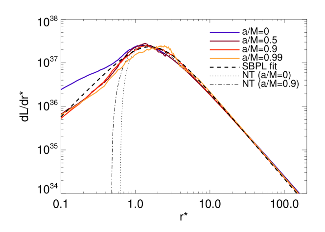
Figure 4: Luminosity profile $dL/dr^{\ast}$, for a range of spins, all normalized to give a bolometric luminosity of $L=0.1L_{\rm Edd}$ for a black hole mass of $10M_{\odot}$. The solid curves correspond to the emitted luminosity, i.e., the black solid curves of Fig. 3. The black dashed curve is the best-fit smoothly-broken power law (SBPL) function defined in Appendix A, and the dotted (dot-dashed) curve corresponds to a NT disk with $a/M=0$ ($0.9$).

In Figure 4 we show the emission profiles of the four different MHD simulations posed in terms of the dimensionless radial coordinate $r^{\ast}$. As expected, they all peak around $r^{\ast}\approx 1.5$, and at large $r^{\ast}$, they all approach the Newtonian large-radius limit $dL/dr\propto r^{-2}$. We also show a simple analytic fit to the emissivity profile, which takes the form of a smoothly-broken power law with inner slope of $dL/dr^{\ast}\propto r^{\ast 7/4}$ (SBPL; dashed curve), as well as the corresponding profiles for Novikov-Thorne disks ($a/M=0$ dotted curve, $a/M=0.9$ dot-dashed curve). The local flux from the disk is related to $dL/dr^{\ast}$ through the relation

$$F(r^{\ast})=\frac{1}{4\pi r^{\ast}}\frac{dr^{\ast}}{dr}\frac{dL}{dr^{\ast}}\,.$$ (1)

Along with the emissivity profile, a simple disk model requires a prescription for the fluid velocity. Outside the ISCO, we can use circular, planar geodesic orbits as in Novikov & Thorne (1973). Inside the ISCO, we ignore the fluid’s continuing loss of energy and angular momentum, assuming it follows plunge trajectories with constant specific energy and angular momentum $\varepsilon_{\rm ISCO}$ and $\ell_{\rm ISCO}$.

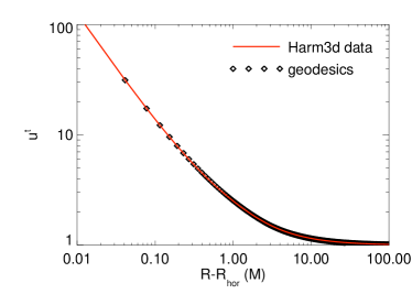
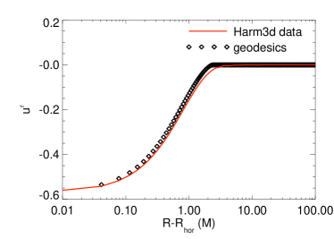
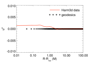
Figure 5: Velocity components as a function of radius for spin parameter $a/M=0.5$. The solid red lines come from the time- and azimuth-averaged simulation data, sampled in the disk midplane. The diamond points correspond to the analytic model for circular, planar geodesic orbits outside the ISCO and plunging trajectories with constant energy and angular momentum. Note the extremely small magnitude of $u^{\theta}$ found in the simulation.

In Figure 5 we show how well these geodesic orbits agree with the time- and azimuth-averaged velocities from the $a/M=0.5$ simulation data sampled in the midplane. To emphasize the behavior in the plunging region, we plot $u^{\mu}$ vs $r-r_{\rm horizon}$ (Boyer-Lindquist coordinates). The $a/M=0.5$ case demonstrates that we accurately capture spin effects while also including a non-negligible plunge region; for $a/M=0.99$ almost the entire disk (described in Boyer-Lindquist coordinates) is outside the ISCO and thus on circular orbits.

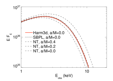
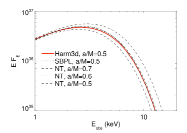
Figure 6: Thermal spectra from accreting black holes with spins $a/M=0$ and $a/M=0.5$. In both cases, the black hole mass is $10M_{\odot}$, the accretion rate is $\dot{m}=0.1$ (assuming the radiative efficiency of the “true” spin), and the observer inclination is $i=60^{\circ}$. The spectra come from Harm3d simulation data (solid red curves) and the phenomenological SBPL model (dotted black curves). Novikov-Thorne spectra for a few representative spins are shown as thin dashed curves. The NT spin cases increase in luminosity with increasing spin.

4 Implications for Parameter Inferences

With these convenient analytic models for the thermal disks, we can revisit the question asked in Noble et al. (2011) and Kulkarni et al. (2011), i.e., “How best to fit data in order to infer the spin of the black hole?” It would be prohibitively expensive computationally to construct a set of MHD simulations with sufficiently fine spacing in black hole spin to support realistic data-fitting. However, our approximate analytic model is easily adapted to such an effort. To validate this approach, we first demonstrate that the spectra predicted by this model closely match the spectra predicted from actual MHD simulations. Given the local emissivity and the four-velocity at each point in the disk, whether taken from simulations or the model, we use the relativistic radiation transport code Pandurata to generate spectra as seen by a distant observer; we then compare the result. Note that Pandurata includes polarization and limb-darkening emissivity governed by electron scattering in the disk atmosphere (Chandrasekhar, 1960). We also include the effects of returning radiation—photons that scatter off the opposite side of the disk after getting deflected by the extreme gravitational lensing of the black hole (Schnittman & Krolik, 2013).

In Figure 6 we show two examples of how well our model reproduces actual simulation predictions for the disk’s thermal spectrum, and how both differ from the NT model. In the left panel, we show the results from the $a/M=0$ simulation as a solid red curve, and in the right panel, the same for $a/M=0.5$. The NT spectra for a few comparable spins are plotted as dashed lines, and the SBPL spectra for the “correct” spins are shown as dotted lines. In both cases, the SBPL prediction adheres very closely to the prediction directly from MHD data. However, when the NT model uses the correct spin, it under-predicts the luminosity at energies above the spectral peak by $\sim 10\%$. As we will see below, when the NT model best fits, its spin is too large.

We caution the reader that these contrasts are taken assuming all the other parameters that must be inferred from measurements (the black hole distance $D$, mass $M$, and accretion rate $\dot{M}$) are their correct values. Although this cannot in general be guaranteed, their effect on the spectrum is to alter the overall normalization and peak energy of the spectrum, but the shape of the spectrum—especially above the thermal peak—is a function only of the spin and inclination.

4.1 $\chi^{2}$ fits to the spectrum:fixed inclination angle

To determine quantitatively how use of our new model affects parameter inference, we adopt a simple fitting procedure in which the MHD spectrum is treated as observational data with an error on each energy bin proportional to the square root of the number of photons in that bin, then carry out a least-squares fit with a suite of NT and SBPL spectra. Rather than specify a photon count rate and detector response function, we simply assume a total of $10^{6}$ photons, deposited appropriately through ten energy channels. Initially, we hold the observer inclination fixed, but the black hole mass, accretion rate, and distance are allowed to vary freely to minimize $\chi^{2}$. The results are shown in Table 2 for target parameters of $M=10M_{\odot}$, $\dot{m}=0.1$, and under the assumption that all the cooling power is efficiently converted into thermal flux at the disk surface.

Table 2: Spin fitting, $E=2-10$ keV

$a/M$	$i$ (deg)	best fit	best fit
		Novikov-Thorne	SBPL emission
0.0	15	0.20	0.10
	45	0.20	0.05
	75	0.30	0.10
0.5	15	0.60	0.55
	45	0.55	0.50
	75	0.60	0.50
0.9	15	0.95	0.87
	45	0.92	0.85
	75	0.93	0.87
0.99	15	.997	.991
	45	.992	.980
	75	.991	.980

These results are in agreement with the findings of Noble et al. (2011), finding a modest but consistent overestimate of the spin parameter when fitting to a NT disk model. Kulkarni et al. (2011) also found a systematic error due to assuming the NT model, but of slightly smaller magnitude than both Noble et al. (2011) and the new results presented here. Some possible explanations for these differences were outlined in detail in Noble et al. (2011). One potential distinction mentioned there was the difference between averaging over $t$ and $\phi$ before or after calculating the spectra. We will discuss this issue in more detail below in Section 4.2, but for the purposes of facilitating direct comparison with Kulkarni et al. (2011), the fits in table 2 were done after averaging the simulation data over time and azimuth, then carrying out a single ray-tracing spectral calculation.

The fits quoted in Table 2 were carried out over the energy range 2–10 keV, appropriate for the large body of archival data from black holes in the thermal state. From Figure 6, it is clear that this energy range is also ideal for distinguishing between different spins for systems with comparable masses and luminosities to the fiducial $M=10M_{\odot}$ and $\dot{m}=0.1$. When performing the fits over a wider energy range 0.1–10 keV, the outer disk contributes greater weight, yet this part of the spectrum is nearly independent of black hole spin, so the net effect is almost negligible, and we find nearly identical values for the best-fit spins.

Not surprisingly, the SBPL model does a better job at recovering the spin parameter for the target spectra, particularly for smaller values of the spin, where emission from the ISCO region is relatively more important. The small variations from perfect fitting are likely due to the stochastic nature of the MHD simulations as described above. There does not appear to be any clear trend for systematic offsets with observer inclination. Taken together, the deviations between the target spins and the best-fit SBPL spins can be taken as a rough estimate for the systematic error in the spin fitting method. Comparing with Table 1, it is clear that the radiative efficiency alone is not a sufficient measure of the thermal emissivity: the MHD simulations give efficiencies that are very similar to NT, but the shapes of the observed thermal spectra show deviations from the classic thin disk model. And ultimately, it is the spectral shape that is observed, not the radiative efficiency.

4.2 $\chi^{2}$ fits to the spectrum: unknown inclination angle

As shown in Figure 6, the shape of the thermal spectrum in the $2-10$ keV band is a function of the black hole spin. For a fixed bolometric luminosity, a larger spin leads to a higher disk temperature because the total radiative power is emitted from a smaller region. However, relativistic beaming and Doppler blue-shifting of photons emitted from a highly inclined disk have a similar hardening effect on the observed spectrum. Together, there is an almost perfect degeneracy between the black hole spin and the observer inclination angle. To demonstrate this, we plot in Figure 7 contours of $\Delta\chi^{2}$ between a simulated target spectrum generated from the MHD data with $i=60^{\circ}$ and $a/M=0.5$, and a template of fitting spectra based on the SBPL model. The simulated spectral data have Poisson error bars consistent with an observation of roughly $10^{6}$ photons divided into 10 energy bins, typical of what might be expected from a first-generation X-ray polarimeter (Jahoda et al., 2014; Weisskopf et al., 2013).

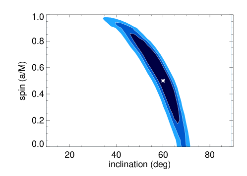
Figure 7: Contours of $\Delta\chi^{2}$ for simulated spectral observations of an accreting black hole in the thermal state. The spectrum is fit in the range $2-10$ keV with energy resolution of $\Delta E/E\sim 0.2$. The target system (marked by ’*’) has spin parameter $a/M=0.5$, inclination $i=60^{\circ}$, mass $M=10M_{\odot}$, and luminosity $L=0.1L_{\rm Edd}$. The contours represent 1-, 2-, and 3-$\sigma$ confidence limits.

This degeneracy is a well-known problem with the continuum fitting method, and is generally resolved by assuming a specific inclination derived from the optical light curve of the distorted stellar companion (Orosz et al., 2002; Remillard & McClintock, 2006). One systematic problem with this approach is that the inclination of the inner disk may very well be misaligned with the inclination of the binary orbit (Li et al., 2009).

Another important issue in fitting observations is properly treating the scattering atmosphere of the accretion disk. Because the electron scattering opacity dominates over free-free absorption for the temperatures and densities expected in the inner disk, we expect a Wien spectrum for the local emission (Rybicki & Lightman, 2004). For fitting our simulated spectra to NT or SBPL models, motivated by Shimura & Takahara (1995) we used a simple hardening factor of 1.8 as in Noble et al. (2011). When fitting real observational data, McClintock et al. (2014) find that more detailed atmospheric models are required to achieve a good fit (Davis & Hubeny, 2006).

As mentioned above in Section 3, there is also the issue of t- and $\phi$-averaging the data before carrying out the ray-tracing calculation. This averaging has the effect of softening the observed spectrum. Consider an annulus of the disk with a uniform temperature $T_{0}$. If instead, the total thermal flux were emitted from a series of discrete hotspots of temperature $T_{h}$ and covering fraction $C_{h}$, while maintaining the same total flux, the new spectrum is a higher-temperature blackbody with color-correction factor $f_{c}=C_{h}^{-1/4}$.

As a test of this effect, we generated spectra both before and after averaging in time and azimuth, and find that by first averaging the simulation data and using a color-correction factor of $f_{c}=1.8$, we can exactly match the spectra that result from using the full time-varying 3D data with $f_{c}=1.6$ and then integrating the light curves in time and azimuth. Of course, Nature uses the latter method, so if the observational data best fits an azimuthally symmetric model best with a certain hardening function, one must keep in mind that this in fact corresponds to a somewhat softer local spectrum coming from an inhomogeneous disk. Careful analysis of X-ray timing properties may be one promising way of breaking this degeneracy and lead to greater understanding of the properties of the accretion disk atmosphere.

4.3 $\chi^{2}$ fits to the X-ray polarization

As discussed in detail in Schnittman & Krolik (2009), X-ray polarization observations of black holes in the thermal state provide a powerful new way to probe the dynamics of the inner accretion flow, and thereby measure the black hole spin. Chandrasekhar (1960) showed that the photons emitted from a plane-parallel, scattering-dominated atmosphere are polarized in a direction parallel to the emitting surface. The degree of polarization ranges from 0 for face-on observers up to $11\%$ for edge-on observers. Because of relativistic effects such as beaming and gravitational lensing, the net polarization of light from the inner regions of an accretion disk is reduced in magnitude, and the angle of polarization is rotated. Because higher-energy photons come from the inner regions, these relativistic effects are energy dependent, and thus the polarization spectrum can be used to probe the inner disk.

This technique was first proposed over thirty years ago by Connors et al. (1980), who considered only direct radiation from the accretion disk. Schnittman & Krolik (2009) included the effects of returning radiation, photons emitted from the disk, deflected by the black hole, and reflected off the far side of the disk before reaching the distant observer. These photons are strongly polarized by the large-angle scattering geometry and impart a significant polarization signature to the total radiated flux.

For the purpose of analyzing the X-ray polarization, we define the black hole spin axis to be along the vertical direction, so a polarization angle of $\psi=0^{\circ}$ is parallel to the disk. This is the case for the low-energy photons emitted at large radii, where relativistic effects are negligible. The high-energy photons emitted close to the black hole are more likely to contribute to the returning radiation and scatter into the vertical polarization mode. Since the disks around rapidly spinning black holes extend closer to the horizon, they should exhibit more vertical polarization, and the transition from horizontal to vertical polarization occurs at a lower energy.

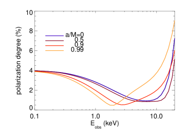
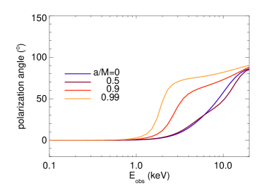
Figure 8: Polarization amplitude (top) and angle (bottom) for thermal disks as a function of photon energy for a range of black hole spins. In all cases, the black hole parameters are $M=10M_{\odot}$, $L=0.1L_{\rm Edd}$, and $i=75^{\circ}$.

In Figure 8 we plot the angle and degree of polarization from the MHD simulation data as a function of photon energy for our fiducial parameters $M=10M_{\odot}$, $L=0.1L_{\rm Edd}$, and $i=75^{\circ}$. The spectropolarization signal is clearly sufficient to distinguish between different spins with even modest energy resolution. The near overlap of the $a/M=0$ and $a/M=0.5$ curves is due to the anomalously low (high) flux from the $a/M=0.5$ ($a/M=0$) simulations, as described above. Real observations would cover a much longer duration of time, smoothing out the stochastic variability seen in the much shorter simulations.

Polarization also provides a complementary observable that can break the spin-inclination degeneracy inherent in the traditional spectral continuum fitting method Li et al. (2009). To demonstrate its power, we perform the same sort of spectral fitting shown in Figure 7, but using the broad-band polarization information displayed in Figure 8. Instead of the intensity spectrum, we use the energy-dependent Stokes parameters $Q_{\nu}$ and $U_{\nu}$, as in Schnittman & Krolik (2009). Again, we use a simulated spectrum from a target disk with $a/M=0.5$ and $i=60^{\circ}$. For a broad-band photoelectric polarimeter like PRAXyS (Jahoda et al., 2014), $10^{6}$ photons divided roughly equally between 10 energy bands gives a 1-$\sigma$ uncertainty on the polarization degree of about $1\%$ per band. Fitting the polarization information with the SBPL model between 2-10 keV, we get the confidence contours shown in Figure 9. At 2 keV there is still significant returning radiation, so the polarization signal is not a perfect probe of disk inclination. A soft X-ray polarimeter sensitive over the 0.1-0.5 keV band would significantly improve sensitivity to disk inclination.

The slight spin-inclination degeneracy seen in Figure 9 can be understood as follows. From Figure 8 it is clear that the location of the transition from horizontal to vertical orientation occurs at lower energy for increasing spin. This transition is due to a small number of highly polarized returning photons dominating over the vast majority of weakly polarized direct photons. At higher inclinations, the direct signal is more highly polarized, so is harder to overcome with returning photons, and thus the transition point shifts to higher energy where the contribution from returning radiation is higher. Therefore, to maintain a constant transition energy, increasing inclinations require a higher spin.

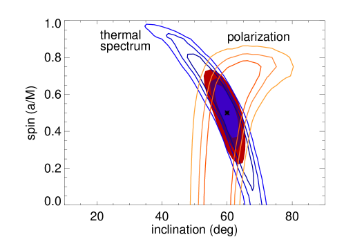
Figure 9: Contours of confidence limits as in Figure 7, but now also considering polarization spectra $Q_{\nu}$ and $U_{\nu}$. The simulated sensitivity corresponds to a minimum detectable polarization of $\sim 1\%$.

Comparing the contours in Figure 9, we see that the degeneracy due to continuum fitting and that due to polarization intersect at a significant angle. As a result, the range of both parameters consistent with a good fit is substantially reduced. Clearly, X-ray spectropolarimetry observations have the potential to be of great benefit to measurements of black hole spin and inclination.

For all of the contours in Figure 9, we used the SBPL model for the radial emissivity profile. When redoing them with a NT model as in Noble et al. (2011), not surprisingly we get very similarly shaped contours for $\Delta\chi^{2}$, but with a systematic offset towards higher spin. However, we find that the actual minimum in $\chi^{2}$ is consistently lower for the SBPL model than for NT. For the fiducial observations used above with $10^{6}$ photons over the 2-10 keV band, combined spectral and polarization fits to the MHD data prefer the SBPL model at roughly $90\%$ confidence. For a photon-limited (as opposed to background-limited) detector, this significance would simply grow with more and longer observations. Thus, X-ray polarimetry combined with X-ray spectroscopy can also be a significant aid in distinguishing different emissivity profiles, thereby creating a new diagnostic of accretion dynamics in the innermost regions of accretion disks around black holes.

5 Summary

We have carried out a new series of high-resolution GRMHD simulations of thin accretion disks around spinning black holes. Using a physically motivated cooling function to emulate radiative losses, we have found a single broken power-law model that accurately describes the luminosity profile of the thermal emission from these disks. By reframing the profile in terms of a new radial coordinate, this model can capture the additional emissivity near the ISCO produced by MHD stresses, but omitted by the traditional Novikov-Thorne model. These new profiles should more accurately fit the 2-10 keV spectra observed from stellar-mass black holes in the thermal state, thereby reducing systematic errors in parameter estimates of black hole spin and inclination. Although a single power-law index for the inner radial dependence of the surface brightness fits all our simulations quite well, it is possible that this index might be altered if, for example, the magnetic field topology were different.

We have further found that the polarization induced by returning radiation (Schnittman & Krolik, 2009) offers a powerful probe for tightening these parameter inferences. It constrains both the spin and the inclination in a way having little degeneracy with the spectral method. At the same time, it can also constrain the detailed shape of the intrinsic disk radial luminosity profile (including the possibility of a different inner power-law index). Moreover, because the trajectories of the returning radiation photons pass close to the black hole’s photon orbit, this method probes as deeply into the regime of strong-field relativistic gravity as almost any imaginable observational method.

Appendix A Emissivity Function

Here we present a simple procedure for generating the phenomenological emissivity profile that best matches the MHD simulations, for a range of black hole spin parameters.

We begin by defining a new radial coordinate that captures the effects of increased proper distance as measured by a geodesic observer near the black hole:

$$d\tilde{r}\equiv g_{rr}^{1/2}dr=\left(1-\frac{2}{r}+\frac{a^{2}}{r^{2}}\right)^{1/2}dr\,,$$ (A1)

with $dr$ the standard differential radial coordinate in Boyer-Lindquist coordinates. Integrating equation (A1) gives $\tilde{r}$ as a function of $r$ with the condition that they are equal when $r=(3/2)r_{\rm ISCO})$.

We next scale by the ISCO radius to define another coordinate $r^{\ast}\equiv\tilde{r}/r_{\rm ISCO}$. With these coordinates, the universal emissivity function can be written as a smoothly-broken power law of the form

$$\frac{dL}{dr^{\ast}}=Cr^{\ast\,\varphi}\left[\frac{\cosh(\ln(r^{\ast}/R_{0})/\Delta R)}{\cosh(\ln(1/R_{0})/\Delta R)}\right]^{\xi\,\Delta R}\,,$$ (A2)

where $C$ is an overall normalization factor, $R_{0}$ is the location of the power-law break, $\Delta R$ is the width of the break, and $\alpha$ and $\beta$ are the slopes of the power law at small and large radii respectively, with $\varphi=(\beta+\alpha)/2$ and $\xi=(\beta-\alpha)/2$. We fix $\beta=-2$ to give the proper behavior at large $r$, and $C$ is determined by the total mass accretion rate. For the remaining free parameters, we find the best simultaneous fit with $\alpha=1.73$, $R_{0}=1.68$, and $\Delta R=0.92$.

From equations (A2) and (1) above, we can write the local flux as

$$F(r^{\ast})=\frac{1}{4\pi r^{\ast}}\frac{dr^{\ast}}{dr}\frac{dL}{dr^{\ast}}\,.$$ (A3)

For purely blackbody emission, the local temperature is then given by $T(r)=[F(r)/(2\sigma)]^{1/4}$. The normalization factor $C$ in (A2) is simply a function of the total luminosity: $L=\int_{0}^{\infty}dr^{\ast}(dL/dr^{\ast}$ and scales linearly with the mass accretion rate. The black hole mass $M$ comes in when converting the dimensionless coordinate $r^{\ast}$ to cgs units, leading to a factor of $M^{-2}$ in equation (A3), giving the familiar scaling of disk temperature $T\sim M^{-1/2}\dot{M}^{1/4}$.

Outside of the ISCO, the gas moves in planar, circular orbits with specific energy and angular momentum

$$\varepsilon_{\rm circ}(r) = \frac{r^{2}-2r+ar^{1/2}}{r(r^{2}-3r+2ar^{1/2})^{1/2}}$$ (A4a)

$$\ell_{\rm circ}(r) = \frac{2}{3^{1/2}}\frac{3r^{1/2}-2a}{r^{1/2}}\,.$$ (A4b)

In the plunging region, the gas follows geodesics with constant energy $\varepsilon(r_{\rm ISCO})$ and angular momentum $\ell(r_{\rm ISCO})$. From these, the coordinate 4-velocity is given by

$$u^{t} = -\varepsilon\,g^{tt}+\ell\,g^{t\phi}$$ (A5a)

$$u^{r} = u_{r}g^{rr}$$ (A5b)

$$u^{\theta} = 0$$ (A5c)

$$u^{\phi} = -\varepsilon\,g^{t\phi}+\ell\,g^{\phi\phi}$$ (A5d)

where we can solve for the radial momentum $u_{r}$ from the mass-shell normalization condition:

$$u_{r}=-\sqrt{\frac{1+\varepsilon^{2}g^{tt}-2\varepsilon\ell g^{t\phi}}{g^{rr}}}\,.$$ (A6)

This simple procedure works well to construct physically-motivated models for thin accretion disks for all spins up to $a/M\approx 0.997$. Above that limit, the coordinate $r^{\ast}$ takes on negative values outside of the ISCO. For extreme spins above this value, we recommend following the traditional Novikov-Thorne emissivity models, which in any case have almost no remaining plunging region between the ISCO at $r=1.28M$ and the horizon at $r=1.08M$.

References

- Avara et al. (2015) Avara, M.J., McKinney, J.C. & Reynolds, C.S., arXiv:1508.05323
- Beckwith et al. (2008) Beckwith, K., Hawley, J. F., & Krolik, J. H. 2008, MNRAS 390, 21
- Chandrasekhar (1960) Chandrasekhar, S. 1960, Radiative Transfer, Dover, New York
- Connors et al. (1980) Connors, P. A., Piran, T., & Stark, R. F. 1980, ApJ, 235, 224
- Davis & Hubeny (2006) Davis, S. W., & Hubeny, I. 2006, ApJS, 164, 530
- Davis et al. (2011) Davis, S.W. 2011, ApJ, 734, 111
- De Villiers & Hawley (2003) De Villers, J.-P. & Hawley, J.F. 2003, ApJ, 592, 1060
- Gammie (1999) Gammie, C.F. 1999, ApJL, 522, 57
- Gammie et al. (2003) Gammie, C.F., McKInney, J.C. & Tóth, G. 2003, 589, 444
- Gammie et al. (2004) Gammie, C. F., Shapiro, S.Ł., & McKinney, J. 2004, ApJ 602, 312
- Gou et al. (2011) Gou, L. et al. 2011, ApJ, 742, 85
- Gou et al. (2014) Gou, L. et al. 2014, ApJ, 790, 29
- Hawley et al. (2011) Hawley, J.F., Guan, X. & Krolik, J.H. 2011, ApJ, 738, 84
- Hirose et al. (2009) Hirose, S., Krolik, J.H. & Blaes, O.M. 2009, ApJ, 691, 16
- Jahoda et al. (2014) Jahoda, K. M., et al. 2014, Proceedings SPIE, 9914, 0N
- Jiang et al. (2013) Jiang, Y.-F., Stone, J.M. & Davis, S.W. 2013, ApJ, 778, 65
- Krolik et al. (2005) Krolik, J. H., Hawley, J. F., & Hirose, S. 2005, ApJ 622, 1008
- Kulkarni et al. (2011) Kulkarni, A. K., et al. 2011, MNRAS, 414, 1183
- Li et al. (2009) Li, L. X., Narayan, R., & McClintock, J. E. 2009, ApJ 691, 847
- McClintock et al. (2011) McClintock, J. E., et al. 2011, Class. Quantum Grav., 28, 114009
- McClintock et al. (2014) McClintock, J. E., Narayan, R., & Steiner, J. F. 2014, Space Science Rev. 183, 295
- McKinney et al. (2012) McKinney, J. C., Tchekhovskoy, A., & Blandford, R. D. 2012, MNRAS, 423, 3083
- Noble et al. (2009) Noble, S. C., Krolik, J. H., & Hawley, J. F. 2009, ApJ 692, 411
- Noble et al. (2010) Noble, S. C., Krolik, J. H., & Hawley, J. F. 2010, ApJ, 711, 959
- Noble et al. (2011) Noble, S. C., Krolik, J. H., Schnittman, J. S., & Hawley, J. F. 2011, ApJ, 743, 115
- Novikov & Thorne (1973) Novikov, I. D., & Thorne, K. S. 1973, in Black Holes, ed. C. DeWitt & B. S. DeWitt (New York: Gordon and Breach)
- Orosz et al. (2002) Orosz, J. A. 2002, ApJ 568, 845
- Penna et al. (2010) Penna, R.F. 2010, MNRAS, 408, 752
- Remillard & McClintock (2006) Remillard, R. A., & McClintock, J. E. 2006, ARA& A, 44, 49
- Rybicki & Lightman (2004) Rybicki, G. B., & Lightman, A. P. 2004, Radiative Processes in Astrophysics (Weinheim: Wiley-VCH)
- Schnittman & Krolik (2009) Schnittman, J. D., & Krolik, J. H. 2009, ApJ 701, 1175
- Schnittman et al. (2013) Schnittman, J. D., Krolik, J. H., & Noble, S. C. 2013, ApJ 769, 156
- Schnittman & Krolik (2013) Schnittman, J. D., & Krolik, J. H. 2013, ApJ 777, 17
- Shimura & Takahara (1995) Shimura, T., & Takahara, F. 1995, ApJ, 445, 780
- Soltan (1982) Soltan, A. 1982, MNRAS 200, 115
- Sorathia (2012) Sorathia, K.A., Reynolds, C.S., Stone, J.M. & Beckwith, K. 2012, ApJ, 749, 189
- Steiner et al. (2011) Steiner, J.F. et al. 2011, MNRAS, 416, 941
- Thorne (1974) Thorne, K. S. 1974, ApJ 191, 507
- Weisskopf et al. (2013) Weisskopf, M. C., et al. 2013, Proceeding SPIE, 8859, 08
- Zhu (2012) Zhu, Y. et al. 2012, MNRAS, 424, 2504