The iron dispersion of the globular cluster M 2, revised

Abstract

M2 has been claimed to posses three distinct stellar components that are enhanced in iron relative to each other. We use equivalent width measurements from 14 red giant branch stars from which Yong et al. detect a $\sim$0.8 dex wide, trimodal iron distribution to redetermine the metallicity of the cluster. In contrast to Yong et al., which derive atmospheric parameters following only the classical spectroscopic approach, we perform the chemical analysis using three different methods to constrain effective temperatures and surface gravities. When atmospheric parameters are derived spectroscopically, we measure a trimodal metallicity distribution, that well resembles that by Yong et al. We find that the metallicity distribution from Fe ii lines strongly differs from the distribution obtained from Fe i features when photometric gravities are adopted. The Fe i distribution mimics the metallicity distribution obtained using spectroscopic parameters, while the Fe ii shows the presence of only two stellar groups with metallicity [Fe/H]$\simeq$–1.5 and –1.1 dex, which are internally homogeneous in iron. This finding, when coupled with the high-resolution photometric evidence, demonstrates that M 2 is composed by a dominant population ($\sim$99%) homogeneous in iron and a minority component ($\sim$1%) enriched in iron with respect to the main cluster population.

1 Introduction

Most of the globular clusters (GCs) surveyed so far show large internal variations in the abundances of light elements (C, N, O, Na, and Al; i.e., Kraft, 1994, Gratton, Sneden & Carretta, 2004, Carretta et al., 2009a, Carretta et al., 2009b). In contrast, only a small subset of the cluster population is characterised by star-to-star variations in their heavy-element content (e.g. Gratton, Carretta & Bragaglia, 2012).

Among clusters with intrinsic spreads in heavy elements, of great interest are those characterised by a dispersion in their slow ($s$)-capture element abundance content (namely; NGC 1851, M 22, NGC 362, M 2, NGC 5286, and M 19). In these GCs, stars are clustered in two groups with different $s$-process element content. Stars with higher $s$-process element content in M 22 (Marino et al., 2009, 2011), M 2 (Yong et al., 2014b), NGC 5286 (Marino et al., 2015), NGC 1851 (Yong & Grundahl, 2008; Carretta et al., 2010b, but see Villanova, Geisler & Piotto, 2010), and M 19 (Johnson et al., 2015) are also believed to be more metal-rich than stars with no $s$-process element overabundance, the characteristic range in iron being $\simeq$ 0.2–0.4 dex. Also, the $s$-process bimodality is associated to the photometric split in the sub-giant branch (SGB) in $V,V-I$ colour-magnitude diagrams (CMDs; Milone et al., 2008; Piotto, 2009; Piotto et al., 2012) and to the multimodal red giant branch (RGB) when a combination of colours, including the $U$ filter is used to construct the CMD (Marino et al., 2012; Carretta et al., 2010b; Lardo et al., 2012, 2013; Yong et al., 2014b; Carretta et al., 2013; Marino et al., 2015).

The presence of internal variations in iron would suggest that clusters with Fe spreads have been able to keep high-energy supernova (SN) ejecta. This in turn indicates that M 22, M 2, NGC 5286, NGC 1851, and M 19 were much more massive at their birth, possibly being nuclei of dwarfs disrupted by Milky Way tidal fields (e.g. Marino et al., 2015, but see also Pfeffer et al., 2014), as SN ejecta are too energetic to be retained by less massive systems like Galactic GCs, which have typical masses less than or equal to a few times 10⁵ M_⊙ (Baumgardt, Kroupa & Parmentier, 2008). In this scenario GCs showing intrinsic metallicity variations may be considered as former Milky Way satellites, and this assumption greatly impacts on our understanding of how the Galaxy formed and evolved. Therefore, it is crucial to assess whether the observed star-to-star variations are genuine metallicity dispersions.

Iron abundances critically depend on the choice of atmospheric parameters adopted in the spectroscopic analysis. When measuring abundances, two main approaches are routinely used to constrain surface gravities from stellar spectra. When spectra have very good quality; i.e. high signal-to-noise ratio (SNR), wide spectral coverage, relatively large ($\sim$10-20) number of observed Fe ii lines in the covered spectral range, one commonly sets the surface gravity from the ionisation equilibrium of Fe; i.e. in a fashion that the same iron abundance is provided by both Fe i and Fe ii lines. When this approach is not feasible, i.e. in case of spectra with relatively low SNR and/or resolution, very low-metallicity, and/or small spectral coverage; one has to rely on gravities estimated from photometric data, such as those derived using colour-temperature and colour-bolometric correction calibrations or isochrone fitting (e.g. Carretta et al., 2009a, b).

Very recently, Mucciarelli et al., 2015b (Mu15) found that the [Fe ii/H] distribution of M 22 stars is very narrow when the surface gravities are estimated from photometry. Conversely, when gravities are derived from the spectra by imposing the ionisation equilibrium between [Fe i/H] and [Fe ii/H] lines, the iron distribution is $\simeq$ 0.5 dex wide, in agreement with previous results (Marino et al., 2009, 2011). Naively, spectroscopic surface gravities appear more reliable than photometric ones, because they are quantitatively extracted from spectra and they are not estimated form an empirical calibration or stellar evolution, as in the case of photometric gravities. However, Mu15 find that spectroscopic gravities required to match [Fe i/H] and [Fe ii/H] abundances lead to unphysical stellar masses for GC giant stars, with values $\leq$ 0.5 M_⊙. The Mu15 sample is composed by stars in the same evolutionary stage, located at the same distance and with virtually the same age; and their spectroscopic masses are spread over a wide range ($\simeq$0.8 M_☉). Since it is hard to think to a physical mechanism which randomly scatter stellar masses, Mu15 conclude that the Fe spread observed among M 22 stars is artificially produced by the method used to constrain surface gravities.

M 2 is another cluster that has been claimed to posses an intrinsic iron spread, with possibly three populations at [Fe/H]=–1.7,–1.5, and –1.0 dex (Yong et al., 2014b; hereafter Y14). The metal-poor and metal-intermediate components include stars with different $s$-process abundances with stars at [Fe/H]$\simeq$–1.5 dex being $s$-rich (Lardo et al., 2013, Y14) with respect to metal-poor stars at [Fe/H]$\simeq$–1.7 dex. In contrast with other clusters showing $s$-process element bimodality, M 2 is characterised by a third, poorly populated stellar group, which does not show any GC anti-correlations or $s$-process enrichment (Y14).

In their analysis, Y14 take advantage from the wide wavelength coverage and high SNR of their spectra to constrain surface gravities from the ionisation balance. In the light of Mu15 results, we wonder whether the spread observed by Y14 is a genuine iron dispersion and we apply the same analysis as in Mu15 to the spectroscopic sample presented by Yong et al. (2014b) to re-derive iron abundances.

This article is structured as follows: we describe the observational material and data in Section 2. We measure iron abundances in Section 3. We discuss our results in Section 4 and draw our conclusions in Section 5.

Table 1: M 2 stars analysed in this paper, together with the photometric information and the [Fe/H] estimates by Yong et al. (2014b). The stars are grouped according to the classification proposed by Yong et al. (2014b).

ID	$U$	$B$	$V$	$I$	[Fe/H]
	(mag)	(mag)	(mag)	(mag)	(dex)
Metal-poor stars with [Fe/H]$\simeq$ –1.7 dex
NR 37	15.428	14.717	13.556	12.267	–1.66
NR 58	15.838	14.832	13.596	12.243	–1.64
NR 60	15.747	14.828	13.620	12.309	–1.75
NR 76	15.810	15.030	13.906	12.647	–1.69
NR 99	15.816	14.950	13.746	12.433	–1.66
NR 124	15.886	15.217	14.148	12.944	–1.64
Intermediate-metallicity stars with [Fe/H]$\simeq$ –1.5 dex
NR 38	16.457	15.056	13.687	12.339	–1.61
NR 47	–	14.837	13.534	12.116	–1.42
NR 77	–	15.207	13.937	12.704	–1.46
NR 81	16.318	15.101	13.821	12.523	–1.55
Metal-rich stars with [Fe/H]$\simeq$ –1.0 dex
NR 132	16.837	15.534	14.249	12.880	–0.97
NR 207	–	16.055	14.937	13.726	–1.08
NR 254	16.926	16.151	15.073	13.878	–0.97
NR 378	16.621	16.170	15.254	14.207	–1.08

2 Observational material and EW data

The original high-resolution sample analysed in Y14 is composed by 14 RGB stars selected from $uvby$ Strömgren photometry by Grundahl et al. (1999). Five stars (NR 37, NR 38, NR 58, NR 60 and NR 77) were observed using the Magellan Inamori Kyocera Echelle (MIKE) spectrograph (Bernstein et al., 2003) at the Magellan Telescope on 2012 August 26. MIKE spectra cover a wavelength range between $\simeq$3400 to 9000Å, and have a spectral resolution of R = 40 000 in the blue arm and R = 35 000 in the red arm.

The remaining stars were observed with the High Dispersion Spectrograph (HDS; Noguchi et al., 2002) at the Subaru telescope. Echelle spectroscopy was obtained on 2011 August 3 for three stars (NR 76, NR 81, and NR 132). Six additional stars (NR 47, NR 99, NR 124, NR 207, NR 254 and NR 378) were observed using HDS in classical mode on 2013 July 17. The HDS spectrograph was used in the StdYb setting and the 0.8″slit, providing spectra with typical resolution of R $\simeq$ 45 000 and a spectral coverage from $\simeq$4100 to $\simeq$6800 Å. We refer to Y14 for further details on observations and data reduction.

Unpublished Wide-Field Imager (WFI) photometry from one of us was used to identify the targets. Figure 1 shows the position of the spectroscopic targets in the $V$ versus $V-I$, $B$ versus $B-V$ and $U$ versus $U-I$ colour-magnitude diagrams (CMDs). Their magnitudes are listed in Table 1. The photometric catalogue is based on archival $UBVI$ images collected at the WFI at the 2.2 m ESO-MPI telescope and used to select targets for the Gaia ESO survey calibration (Pancino & Gaia-ESO Survey consortium, 2012). The WFI covers a total field of view of 34$\arcmin$ $\times$ 33$\arcmin$, consisting of 8, 2048 $\times$ 4096 EEV-CCDs with a pixel size of 0.238$\arcsec$. These images were pre-reduced using the IRAF package MSCRED (Valdes, 1998), while the stellar photometry was derived by using the DAOPHOT II and ALLSTAR programs (Stetson, 1987, 1992). Details on the preproduction, calibration, and full photometric catalogues will be published elsewhere.

Figure 1 displays the presence of an additional RGB sequence (Lardo et al., 2012, Y14, Milone et al., 2015). We use the same colour code as Y14 to represent stars that have metallicity [Fe/H] $\simeq$ –1.7, –1.5, and –1.0 dex according to their analysis (black circles, red triangles, and aqua squares, respectively). The metal-poor and metal-intermediate stars are tightly aligned along the RGB in the $V$, $V-I$ CMD of Figure 1, while they are clearly separated into two sequences in the split RGBs observed in the $B-V$ and $U-I$ colours. The observed effect can be attributed to the presence of molecular CN and CH absorption in wavelength range covered by the $U$ and $B$ filters (see also Milone et al., 2015). In Lardo et al. (2013) we demonstrate that red RGB stars selected in the $V$, $U-V$ CMD (Lardo et al., 2012) are indeed richer (on average) in both C and N with respect to the stars located on the blue side of the RGB. Both the metal-poor and metal-intermediate components display the light element pattern commonly found in GCs (Y14).

Metal-rich stars (with [Fe/H] $\simeq$–1.0 dex) are located along a redder sequence which runs parallel to the RGB in all the CMDs of Figure 1 because of their higher metallicity with respect to the bulk of M 2 stars (Y14). Metal-rich stars do not show any GC like anticorrelation or $s$-enhancement.

We refer again to Y14 for a complete discussion on cluster membership. Briefly, all stars have colours and magnitudes consistent with being giant stars at the distance of M2 and seven stars have probability P=99% to be cluster members, according the proper motion study by Cudworth & Rauscher (1987). However, the heliocentric radial velocity of M 2 is –5.3 $\pm$2 km s^-1 and the central velocity dispersion is 8.2 $\pm$0.6 km s^-1 (Harris, 1996). Therefore radial velocities alone cannot confirm cluster membership, as field stars could easily have such velocities.

Hubble Space Telescope (HST) photometry by Milone et al. (2015) shows that three metal-rich stars are located on a defined RGB sequence that can be followed down to the SGB and main sequence, supporting the case for cluster membership. However, from Figure 1 we note that star NR 378 is systematically bluer than the other metal-rich stars in all the CMDs of Figure 1. The same is observed in Figure 1 of Y14 in $uvby$ Strömgren colours. In Section 3 we measure for this star a slightly higher metallicity than metal-rich stars. Its location in the CMD and its higher metallicity would indicate NR 378 as a non member, but proper motion or parallaxes are needed to settle the case for this star.

Additionally, Figure 1 suggests that NR 60 could be an asymptotic giant branch (AGB) star, while NR 37 looks slightly off the RGB in Figure 1. To confirm this suggestion, we plotted both stars in the $V,V-I$ CMD (not shown) by Sarajedini et al. (2007). We find that NR 60 is indeed an AGB star (see also Y14), while NR 37 is located on the main RGB body of the cluster in the higher precision HST photometry.

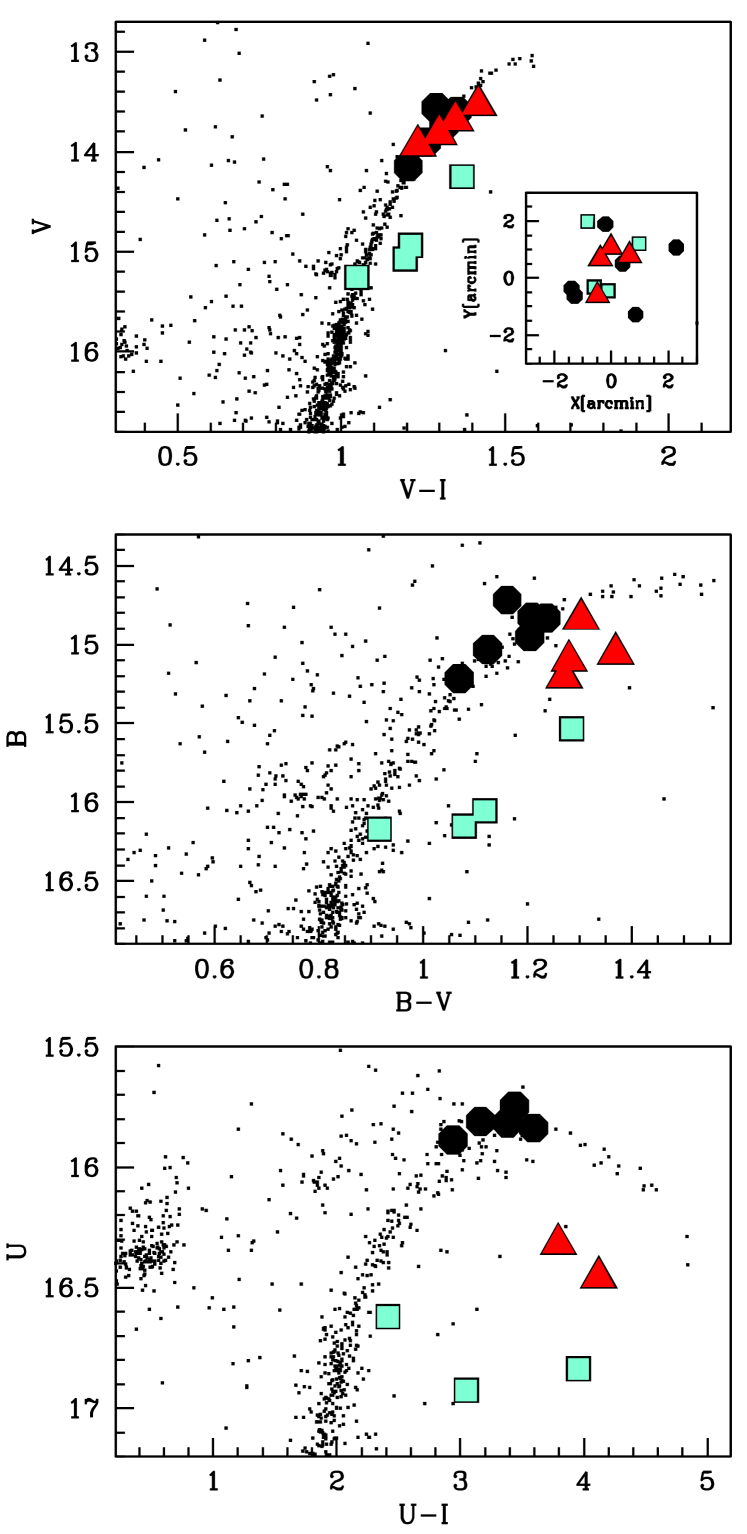
Figure 1: CMDs for $V$ versus $V-I$ (upper), $B$ versus $B-V$ (middle) and $U$ versus $U-I$ (lower) for the spectroscopic targets analysed by Y14 at high spectral resolution. Note that three stars do not have $U$ magnitude in our photometric catalogue. Therefore they are missing in the $U$ versus $U-I$ CMD. The inset in the top panel shows the location of targets across the cluster.The black symbols show metal-poor ([Fe/H]$\simeq$–1.7 dex) stars according to Y14 analysis. The red and aqua symbols denote the metal-intermediate ([Fe/H]$\simeq$–1.5 dex) and metal-rich ([Fe/H]$\simeq$–1.0 dex) components identified by Y14, respectively.

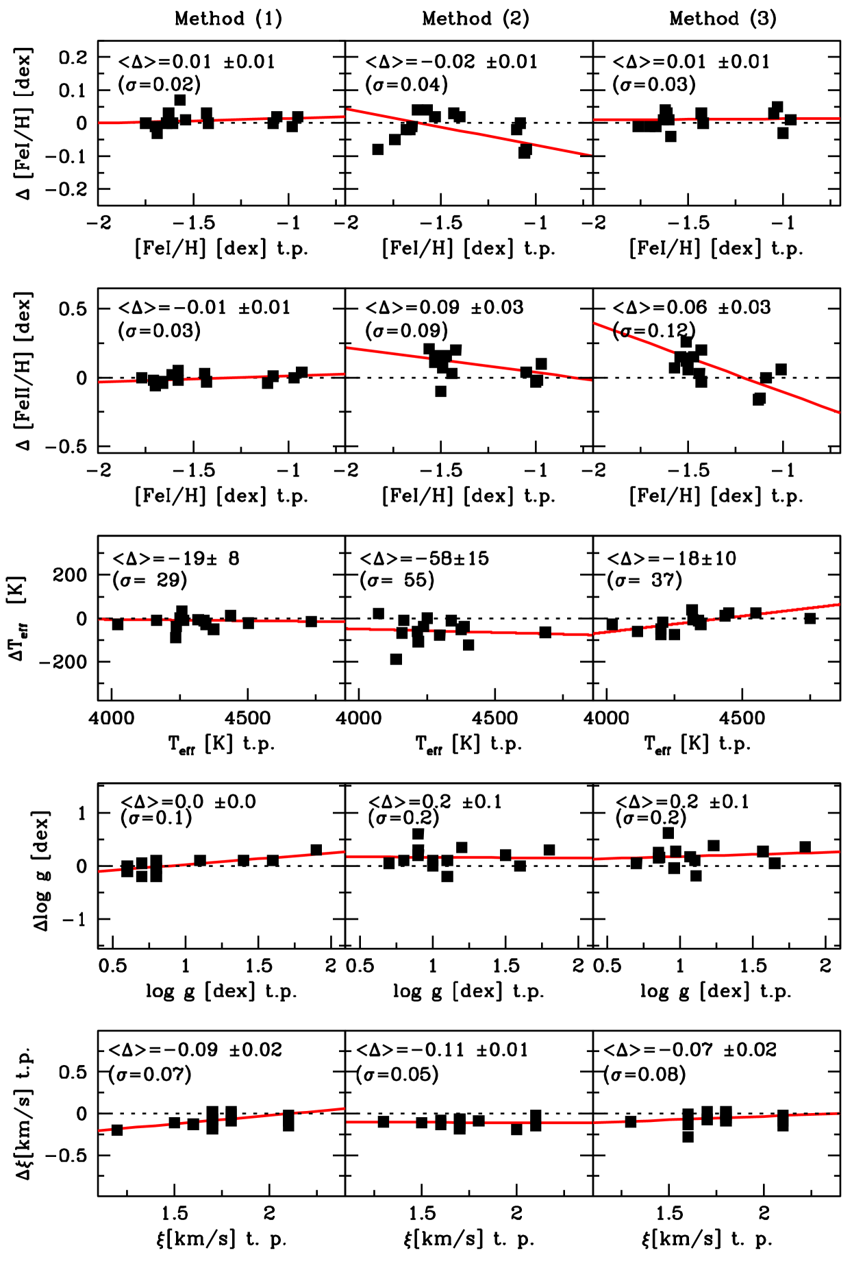
Figure 2: A comparison between the atmospheric parameters adopted in our analysis and those listed in Y14 is presented. Each panel reports in the top left corner the mean difference between (from top to bottom) the [Fe i/H], [Fe ii/H], T_eff, $\log$ g, and $\xi_{\rm{t}}$ measured as detailed in Section 3 and those listed in Y14. Also shown the 1:1 relationships (dotted lines) and the weighted linear fit to the data (solid lines).

Table 2: Atmospheric parameters and metallicities as derived with the methods described in Section 3.

ID	Teff	$\log$ g	$\xi$	[M/H]	[Fe i/H]	$\delta_{\rm{int}}$	$\delta_{\rm{par}}$	[Fe ii/H]	$\delta_{\rm{int}}$	$\delta_{\rm{par}}$
	(K)	(dex)	(kms-1)	(dex)	(dex)	(dex)	(dex)	(dex)	(dex)	(dex)
	(1) Spectroscopic analysis
NR 37	4251$\pm$28	0.60$\pm$0.06	1.70$\pm$0.04	–1.50	–1.63	0.01	0.03	–1.67	0.03	0.05
NR 58	4258$\pm$28	0.80$\pm$0.06	1.80$\pm$0.06	–1.50	–1.57	0.01	0.03	–1.58	0.04	0.06
NR 60	4318$\pm$29	0.30$\pm$0.06	2.10$\pm$0.07	–1.50	–1.75	0.01	0.04	–1.77	0.03	0.05
NR 76	4347$\pm$33	0.70$\pm$0.06	1.60$\pm$0.04	–1.50	–1.70	0.01	0.04	–1.71	0.03	0.05
NR 99	4265$\pm$28	0.60$\pm$0.06	1.80$\pm$0.04	–1.50	–1.69	0.01	0.03	–1.70	0.03	0.05
NR 124	4437$\pm$46	0.80$\pm$0.06	1.80$\pm$0.06	–1.50	–1.64	0.01	0.06	–1.66	0.04	0.06
NR 38	4165$\pm$44	0.60$\pm$0.06	2.10$\pm$0.08	–1.50	–1.61	0.01	0.03	–1.61	0.04	0.07
NR 47	4022$\pm$80	0.70$\pm$0.06	1.70$\pm$0.10	–1.50	–1.42	0.02	0.05	–1.43	0.04	0.13
NR 77	4339$\pm$78	1.10$\pm$0.06	2.10$\pm$0.14	–1.50	–1.43	0.02	0.08	–1.44	0.09	0.09
NR 81	4237$\pm$49	0.80$\pm$0.06	1.70$\pm$0.06	–1.50	–1.54	0.01	0.05	–1.58	0.03	0.07
NR 132	4236$\pm$55	1.40$\pm$0.06	1.70$\pm$0.07	–1.00	–0.98	0.01	0.03	–0.97	0.04	0.09
NR 207	4375$\pm$61	1.40$\pm$0.06	1.20$\pm$0.04	–1.00	–1.06	0.01	0.05	–1.08	0.04	0.08
NR 254	4503$\pm$61	1.90$\pm$0.06	1.50$\pm$0.05	–1.00	–0.95	0.01	0.05	–0.93	0.04	0.08
NR 378	4735$\pm$42	1.60$\pm$0.07	1.70$\pm$0.08	–1.00	–1.08	0.02	0.05	–1.11	0.02	0.05
	(2) Photometric analysis
NR 37	4251$\pm$ 83	0.90$\pm$0.10	1.70$\pm$0.04	–1.50	–1.62	0.01	0.07	–1.53	0.03	0.09
NR 58	4158$\pm$ 76	0.80$\pm$0.10	1.80$\pm$0.06	–1.50	–1.66	0.01	0.06	–1.48	0.04	0.11
NR 60	4218$\pm$ 80	0.90$\pm$0.10	2.00$\pm$0.07	–1.50	–1.83	0.01	0.09	–1.56	0.03	0.08
NR 76	4297$\pm$ 86	1.00$\pm$0.10	1.60$\pm$0.06	–1.50	–1.74	0.01	0.08	–1.53	0.03	0.10
NR 99	4215$\pm$ 80	0.90$\pm$0.10	1.70$\pm$0.04	–1.50	–1.68	0.01	0.07	–1.48	0.04	0.10
NR 124	4387$\pm$ 93	1.20$\pm$0.10	1.70$\pm$0.07	–1.50	–1.65	0.01	0.10	–1.42	0.04	0.09
NR 38	4165$\pm$ 76	0.90$\pm$0.10	2.10$\pm$0.09	–1.50	–1.57	0.01	0.05	–1.47	0.04	0.11
NR 47	4072$\pm$ 69	0.70$\pm$0.10	1.70$\pm$0.10	–1.50	–1.40	0.02	0.05	–1.50	0.04	0.11
NR 77	4339$\pm$ 89	1.10$\pm$0.10	2.10$\pm$0.14	–1.50	–1.43	0.02	0.09	–1.44	0.09	0.10
NR 81	4237$\pm$ 82	1.00$\pm$0.10	1.70$\pm$0.07	–1.50	–1.53	0.01	0.06	–1.49	0.03	0.10
NR 132	4136$\pm$ 74	1.10$\pm$0.10	1.70$\pm$0.06	–1.00	–1.06	0.01	0.03	–1.00	0.04	0.11
NR 207	4375$\pm$ 92	1.50$\pm$0.10	1.30$\pm$0.06	–1.00	–1.08	0.01	0.06	–1.05	0.04	0.11
NR 254	4403$\pm$ 94	1.60$\pm$0.10	1.50$\pm$0.05	–1.00	–1.05	0.01	0.07	–0.99	0.04	0.11
NR 378	4685$\pm$115	1.80$\pm$0.10	1.60$\pm$0.08	–1.00	–1.10	0.02	0.12	–0.97	0.02	0.08
	(3) Hybrid analysis
NR 37	4201$\pm$ 30	0.86$\pm$0.06	1.70$\pm$0.04	–1.50	–1.67	0.01	0.03	–1.50	0.03	0.06
NR 58	4208$\pm$ 30	0.85$\pm$0.06	1.80$\pm$0.06	–1.50	–1.61	0.01	0.03	–1.51	0.04	0.06
NR 60	4318$\pm$ 32	0.92$\pm$0.06	2.10$\pm$0.07	–1.50	–1.76	0.01	0.03	–1.51	0.03	0.05
NR 76	4347$\pm$ 39	1.07$\pm$0.06	1.60$\pm$0.06	–1.50	–1.70	0.01	0.04	–1.54	0.03	0.06
NR 99	4315$\pm$ 29	0.97$\pm$0.08	1.80$\pm$0.04	–1.50	–1.62	0.01	0.03	–1.57	0.03	0.06
NR 124	4437$\pm$ 51	1.23$\pm$0.07	1.80$\pm$0.07	–1.50	–1.63	0.01	0.06	–1.47	0.04	0.06
NR 38	4115$\pm$ 48	0.85$\pm$0.06	2.10$\pm$0.09	–1.50	–1.60	0.01	0.03	–1.43	0.04	0.09
NR 47	4022$\pm$ 80	0.70$\pm$0.06	1.70$\pm$0.10	–1.50	–1.42	0.02	0.05	–1.43	0.04	0.13
NR 77	4339$\pm$ 78	1.10$\pm$0.06	2.10$\pm$0.14	–1.50	–1.43	0.02	0.08	–1.44	0.09	0.09
NR 81	4200$\pm$ 51	0.96$\pm$0.06	1.80$\pm$0.07	–1.50	–1.59	0.01	0.04	–1.50	0.04	0.08
NR 132	4250$\pm$ 30	1.11$\pm$0.06	1.60$\pm$0.09	–1.00	–1.00	0.01	0.02	–1.13	0.03	0.07
NR 207	4450$\pm$ 41	1.57$\pm$0.06	1.30$\pm$0.04	–1.00	–1.03	0.01	0.04	–1.09	0.05	0.06
NR 254	4550$\pm$ 51	1.65$\pm$0.06	1.60$\pm$0.05	–1.00	–0.96	0.01	0.05	–1.12	0.04	0.06
NR 378	4750$\pm$ 52	1.86$\pm$0.07	1.70$\pm$0.10	–1.00	–1.05	0.02	0.06	–1.01	0.02	0.06

3 Iron abundances

In the following, to be consistent with the spectroscopic analysis presented in Y14, we adopt both their equivalent widths (EW) measurements and their atomic line list (see Table 3 in Y14). The main literature sources for Fe i and Fe i atomic data are from the Oxford group, including Blackwell et al. (1979); Blackwell, Petford & Shallis (1979); Blackwell et al. (1980, 1986); Blackwell, Lynas-Gray & Smith (1995), Biemont et al. (1991), and Gratton et al. (2003). We refer to Y14 for additional details on how the atomic line list was compiled and EWs calculated.

We determined iron abundances from Y14 EW measurements with the package GALA (Mucciarelli et al., 2013) based on the width9 code by Kurucz. Model atmospheres were calculated with the ATLAS9 code assuming local thermodynamic equilibrium (LTE) and one-dimensional, plane-parallel geometry; starting from the grid of models available on F. Castelli’s website (Castelli & Kurucz, 2003). For all the models we adopted as input metallicity in the iron abundance derived by Y14. We adjust the input metallicity to the value we find in the subsequent iterations. The ATLAS9 models employed were computed with the new set of opacity distribution functions (Castelli & Kurucz, 2003) and exclude approximate overshooting in calculating the convective flux.

For the abundance analysis, we used only lines with a reduced EW (EWr = $\log$(EW/$\lambda$) between –5.5 (corresponding to $\simeq$20 mÅ for a line at 6300Å) and –4.6 (corresponding to $\simeq$158 mÅ for a line at 6300Å), in order to avoid lines that are both weak and noisy and to exclude lines in the flat part of the curve of growth, respectively. To compute the abundance of iron, we kept only lines within 3$\sigma$ from the median iron value. The adopted reference solar values are from Grevesse & Sauval (1998).

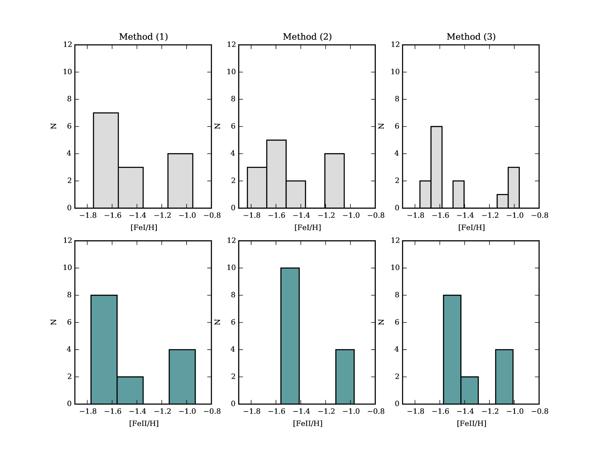
Figure 3: From left to right: Histograms for [Fe i/H] (grey) and [Fe ii/H] (green) obtained from the analysis performed with the spectroscopic, photometric, and the hybrid analysis (method 1, 2, and 3 in Section 3 respectively). Note that histograms represent a severely biased sample and only $\simeq$1-3% of the cluster stars are metal rich (e.g. Milone et al., 2015).

We test how the approach chosen to constrain the stellar effective temperature and surface gravity impacts on the measured [Fe i/H] and [Fe i/H] abundance ratios by performing three independent analysis.

1. Spectroscopic analysis.
   Firstly, we adopt a traditional spectroscopic approach, as done by Y14, in order to verify whether we obtain the same evidence of a metallicity dispersion.

   Atmospheric parameters are constrained as follows. The effective temperature (T_eff) is adjusted until there is no trend between the abundance from Fe i lines and the excitation potential (EP). The surface gravity ($\log$ g) is optimised in order to minimise the difference between the abundance derived from neutral and single ionised iron. Finally, the microturbulent velocity ($\xi_{\rm{t}}$) is established by erasing any trend between the abundance from Fe i and EWr. The same approach to constrain $\xi_{\rm{t}}$ is used consistently in the three independent analysis. The atmospheric parameters are then set in an iterative fashion, first setting the temperature, and then revisiting T_eff as the gravity and microturbulence are tweaked.

   The error associated with the determination of $\xi_{\rm{t}}$ is estimated by propagating the uncertainty in the slope in the rEW versus Fe abundance plane. This uncertainty is of the order of $\simeq$0.07 km sec^-1. The derived T_eff are typically based on more than $\simeq$ 70-130 Fe i lines and have internal uncertainties of about 50-60 K, while the internal uncertainties in log g are of the order of $\simeq$0.06 dex.

   The derived atmospheric parameters and [Fe i/H] and [Fe ii/H] abundances are listed in Table 2, along with their associated uncertainties. The left-hand panel of Figure 2 illustrates how they compare to Y14 results.

   We observe that our T_eff, log g, and $\xi_{\rm{t}}$ estimates are in excellent agreement with those listed in Y14, being the average difference between our and Y14 estimates $\Delta$T_eff=–19 $\pm$ 8 K, $\Delta$$\log$ g=–0.0 $\pm$ 0.0 dex, $\Delta$ $\xi_{\rm{t}}$=–0.09 $\pm$ 0.02 km sec^-1. The agreement between our [Fe i/H] and [Fe ii/H] abundances and those listed in Y14 is also very good. In particular, we note that the metal-poor stars identified by Y14, i.e. see Table 1, are also the most metal-poor stars in our analysis (see Table 2). Additionally, the four stars with [Fe/H]$\simeq$–1.0 dex are the same metal-rich stars in Y14.

   In the left-hand panel of Figure 3, we plotted the histograms of the [Fe i/H] and [Fe ii/H] distributions when the full spectroscopic analysis is performed. Our ability to portrait the [Fe i/H] and [Fe ii/H] distributions for this small dataset critically depends on the adopted bin size ($\Delta$). To adequately represent the shape of the underlying distribution, in Figure 3 we selected $\Delta$ as the value which minimise $C(\Delta)=(2me-va)/\Delta^{2}$; where $me$ and $va$ are the mean and variance of the dataset.

   As one can see, we obtain an iron dispersion that mirrors the dispersion measured by Y14. We find a large ($\Delta$[Fe/H] $\simeq$ 0.8 dex) iron distribution with two prominent peaks at [Fe/H] $\simeq$–1.7 and –1.0 dex and a smaller component at [Fe/H] $\simeq$–1.5 dex. The iron dispersion within the metal-poor stars is larger ($\Delta$[Fe/H] $\simeq$ 0.4 dex) than that expected from observational errors alone, indicating the presence of two separated subpopulations with different metallicity.
   

2. Photometric analysis.
   We use $VI$ WFI photometry to derive photometric T_eff and $\log g_{*}$ estimates. Input T_eff values have been computed by means of the ($V-I$)₀-T_eff transformation by Alonso, Arribas & Martínez-Roger (1999) adopting a colour excess $E(B-V)$ = 0.02 mag taken from the most update version (2010) of the McMaster catalog (Harris, 1996). Surface gravities have been computed assuming the photometric T_eff, the apparent visual distance modulus of 15.50 (Harris, 1996) and an evolutionary mass of 0.82 M_☉ (Bergbusch & VandenBerg, 2001). Assuming that all the stars in M 2 have the same age, the estimated mass for metal-rich stars is 0.85 M_☉. Differences in masses of the order of a few percent of M_☉ have null impact on the metallicity determination (on the order of 0.01 dex or less). The bolometric corrections are calculated according to Alonso, Arribas & Martínez-Roger (1999).

   Uncertainties in T_eff are estimated by taking into account the uncertainty in $V$ and $I$ magnitudes and in the colour excess. The total uncertainty corresponds to a typical uncertainty in T_eff of $\simeq$ 80-90 K. As discussed in Section 2, the star NR 37 appears to lie slightly off the main RGB in our WFI photometry, while it is well located on the main RGB body in the HST photometry by Sarajedini et al. (2007). The observed difference in both $V$ and $I$ magnitudes from are $\Delta V_{{\rm WFI-HST}}$=–0.085 and $\Delta I_{{\rm WFI-HST}}$=–0.051; and lead to a difference of $\simeq$ 50K in the estimate T_eff which is within the errors quoted in Table 2.

   Uncertainties in the surface gravity are derived by considering the error sources in T_eff, luminosity, and mass. Summing all these terms in quadrature leads to a typical uncertainty in $\log g_{*}$ of $\simeq$ 0.08 dex. In the following we assume the (very conservative) error of 0.1 dex in $\log g_{*}$ for all the targets. Milone et al. (2015) found that stars with [Fe/H] = –1.7 dex and very enhanced Na and Al abundances in Y14 are also enhanced in helium up to Y = 0.315 ($\simeq$17% of M 2 stars). According to a set of BASTI isochrones with He-enhancement (Pietrinferni et al., 2004, 2006), for a metallicity [Fe/H]=–1.5 dex and T_eff=4500 K, stars with Y = 0.315 have surface gravity $\simeq$–0.10 dex lower than that derived for stellar models without He-enhancement. Variations up to $\simeq$–0.10 dex in $\log g_{*}$ have negligible impact (of the order $\simeq$ 0.03 dex) on metallicity determinations from Fe ii lines.

   The middle panel of Figure 2 illustrates how (from top to bottom) the measured [Fe i/H], and [Fe ii/H] abundances, T_eff, $\log g_{*}$, and $\xi_{\rm{t}}$ compare to the Y14 results. Again, the agreement between the atmospheric parameters obtained as detailed above and Y14 parameters is very good. On average, we determine slightly lower T_eff and $\xi_{\rm{t}}$ than Y14, i.e. $\Delta$T_eff=–58 $\pm$ 15 K and $\Delta$ $\xi_{\rm{t}}$=–0.11 $\pm$ 0.01 km sec^-1 respectively, while the photometric gravities are on average larger than Y14 ones by $\Delta$$\log$ g=0.2 $\pm$ 0.1 dex ($\sigma$=0.2 dex).

   The middle panel of Figure 2 also shows the difference between neutral and single ionised Fe abundances and Y14 measurements. The Fe i and Fe ii distributions are clearly different. The iron distribution obtained from Fe i lines resembles that obtained with method (1), with a metal rich component at [Fe i/H] $\simeq$–1.0 dex and a metal-poor group with iron abundances in the range between [Fe i/H] = –1.83 to –1.40 dex. The dispersion of [Fe i/H] abundances in the metal-poor stars is larger than those expected from measurement errors alone, indicating the presence of an intrinsic spread. Conversely, the distribution obtained from Fe ii lines is bimodal, with a metal poor ([Fe ii /H] $\simeq$ –1.5 dex) and a metal-rich ([Fe ii /H] $\simeq$ –1.0 dex) components.

   The [Fe i/H] and [Fe ii/H] abundances obtained with this method are listed in Table 2. To better visualise results, we present histograms for the Fe i and Fe ii distributions in the middle panel of Figure 3. The Fe i distribution shows again two main metallicity populations, stars with –1.8 $\leq$ [Fe/H] $\leq$ –1.4 dex showing also an internal iron dispersion. On the other hand, the Fe ii distribution is clearly bimodal. Additionally, the dispersion within each group is consistent with the uncertainties, suggesting the presence of only two population, neither with any intrinsic dispersion.

3. Hybrid analysis.
   Finally, we repeat the analysis adopting spectroscopic temperatures, i.e. T_eff is adjusted until there is no slope between the abundance from Fe i lines and the EP. The advantage of this hybrid analysis is twofold. Firstly, the large number of Fe i lines distributed over a large range of EPs, allows for a very accurate spectroscopic T_eff, with internal uncertainties as small as in the spectroscopic method. Secondly, the T_eff estimated in this fashion are not greatly affected by the uncertainties in the photometry, and in the differential and absolute reddening which impact on the photometric T_eff determination.

   The gravity $\log g_{*}$ is computed through the Stefan-Boltzmann equation according to the new spectroscopic value of T_eff at each iteration. We adopt the same values for the distance modulus, the stellar mass and bolometric corrections as in the photometric analysis.

   Table LABEL:fe2_EW lists all the Fe ii lines used or discarded in our analysis with respect to Yong et al. (2014b) study. Again, atomic data and EWs are from Yong et al. (2014b). Generally, we adopted a more stringent rejection for very weak lines (of the order of $\simeq$15 mÅ), however, the number of lines considered to infer abundances is comparable with Yong et al. (2014b).

   The T_eff and $\xi_{\rm{t}}$ measured in this fashion are again in excellent agreement with Y14, as shown in the right-hand panel of Figure 2. As in the case of method (2), the photometric gravities are on average larger, i.e. $\Delta$ $\log$ g=0.2 dex, than the spectroscopic ones. As for method (2), the new choice of atmospheric parameters does not wipe out the difference between the [Fe i /H] and [Fe ii /H] distributions. The iron abundances measured from [Fe i /H] lines remain very different than those obtained from [Fe ii /H] lines (see Table 2). This is also evident from the right-hand panel of Figure 3, where the neutral and single ionised iron distributions are shown as histograms.

3.1 Uncertainty determinations

Uncertainties on the derived abundances have been computed for each target by adding in quadrature the two main error sources:

1. uncertainties arising from the EW measurements, which have been estimated as the line-to-line abundance scatter divided by the square root of the number of lines used. This term is of the order of 0.01-0.02 dex for Fe i and 0.03-0.05 dex for Fe ii.

2. uncertainties arising from the atmospheric parameters. Those are computed varying by the corresponding uncertainty only one parameter at a time, while keeping the others fixed in the photometric analysis, i.e., case (2). In this case the total uncertainties in [Fe i/H] are of the order of 0.07-0.08 dex, while in [Fe ii/H] are of about 0.10-0.11 dex (due to the higher sensitivity of Fe ii lines to T_eff and $\log$ g).

   When the temperature is spectroscopically optimised, i.e, cases (1) and (3), the uncertainties have been computed following the approach described by Cayrel et al. (2004) to take into account the covariance terms due to the correlations among the atmospheric parameters. For each target, the temperature has been varied by $\pm$ 1 $\sigma$ ${}_{T_{\rm{eff}}}$ , the gravity has been recomputed using the Stefan-Boltzmann equation adopting the new values of T_eff and the v_t derived spectroscopically. The total uncertainties in [Fe i/H] are of the order of 0.05 dex, while in [Fe ii/H] are of about 0.07-0.08 dex.

Table 2 lists both the uncertainty originating from EW measurements ($\delta_{\rm{int}}$), the uncertainty due to atmospheric parameters ($\delta_{\rm{par}}$).

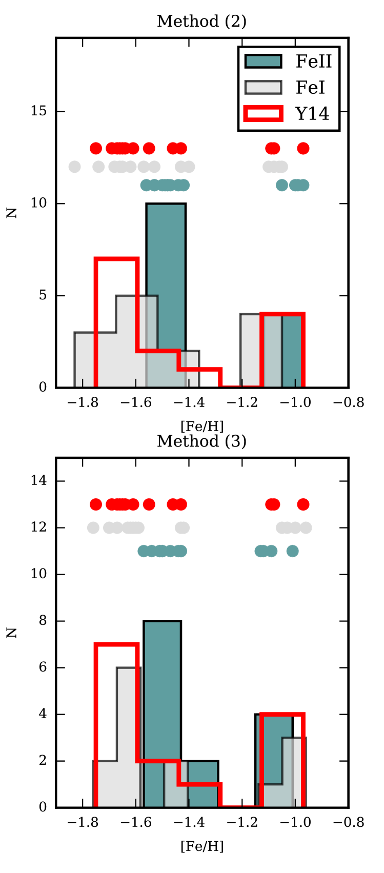
Figure 4: Distribution of Fe i (grey histograms) and Fe ii (green histograms) metallicity from our abundance analysis using the photometric and hybrid approach of Section 3 (top and bottom panels, respectively). For comparison, the metallicity distribution as measured by Yong et al. (2014b) is shown in red. The actual data points used to construct the histogram are shown above the graph.

4 Discussion

The spectroscopic analysis of Section 3 confirms Y14 results: when analysed with atmospheric parameters derived following the traditional spectroscopic approach, the stars with [Fe/H] $\leq$–1.5 dex reveal a clear star-to-star scatter in the iron content. The metallicity distribution from Fe i lines ( grey histograms in Figure 3) is still large with three obvious metallicity sub-populations when photometric gravities are adopted –i.e. methods (2) and (3), while the distribution derived from Fe ii lines is clearly bimodal. The two metallicity components at [Fe ii /H]=–1.5 and –1.1 dex do not show any internal iron spread.

It must be noted that Fe distributions of Figure 3 are not actually representative of the cluster iron distribution. The spectroscopic sample includes four metal-rich and ten metal-poor stars. Metal-rich stars account only for $\sim$1-3% of M 2 stars (Milone et al., 2015), therefore the metal-rich RGB is better sampled than the main RGB in Y14 data. As a result, a Fe ii distribution, weighted based on the fraction of stars observed in the main and metal-rich RGB, would display a large, unimodal component at [Fe ii/H]$\simeq$–1.5 dex and a negligible component ($\leq$3%) at [Fe ii/H]$\simeq$–1.1 dex.

In Figure 4, we plot the Fe i and Fe ii distributions presented by Y14 and the iron distributions we obtained using the photometric and hybrid approach of Section 3. Grey and green symbols are individual measurements for [Fe i/H] and [Fe ii/H], respectively; while red symbols are Y14 [Fe i/H] measurements. Figure 4 shows how the range in metallicity is largely diminished when adopting Fe ii abundances and and photometric gravities. This remains true also when considering different $\log g_{f}$ for the Fe ii (e.g., Meléndez & Cohen, 2009; Raassen & Uylings, 1998; see Figure 5). This demonstrates that the main RGB of M 2 has a homogeneous metallicity of [Fe/H] $\simeq$ –1.5 dex, with a very small spread which is comparable to the star-to-star variations observed in other GCs. On the other hand we confirm the presence of a second metallicity sub-population at higher metallicities.

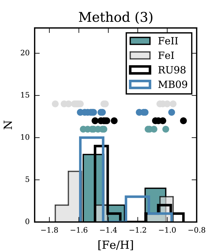
Figure 5: Distribution of [Fe i /H] (grey histogram) and [Fe ii /H] (green histogram) abundance ratios, when using the hybrid analysis of Section 3. The blue and black empty histograms are the distributions for Fe ii lines obtained using different literature sources for $\log g_{f}$ values; Meléndez & Cohen (2009) and Raassen & Uylings (1998) respectively. Note that the Fe ii remains bimodal irrespective on the choice of atomic data. In particular, Fe ii distributions lack the metal-poor tail seen in Fe i histogram.

In the following, we restrict ourselves to the metal-poor component, i.e. stars with [Fe ii/H] $\simeq$–1.5 dex. According to our hybrid analysis, stars NR 76 and NR 77 are both RGB stars with similar atmospheric parameters, i.e. T_eff/$\log$ g/ v_t=4347-4339K/1.07-1.10 dex/1.6-2.10 kms^-1, respectively. Nonetheless, they display very different [Fe i/H] – [Fe ii/H] difference. Star NR 76 has [Fe i/H] – [Fe ii/H]= –0.16 dex, while for star NR 77 [Fe i/H] and [Fe ii/H] lines return basically the same Fe abundance.

NLTE effects lead to a systematic underestimate of the EWs from neutral lines, i.e. Fe i lines. Therefore, the standard LTE analysis of lines formed in NLTE gives lower abundance from neutral lines (Mashonkina et al., 2011). Although the available non local thermodynamic equilibrium (NLTE) calculations do not foresee different corrections for stars with similar atmospheric parameters (e.g. Bergemann et al., 2012), the observed discrepancy between abundances inferred by Fe i and Fe ii lines can be qualitatively explained by the occurrence of some effects driven by overionisation, i.e. affecting mainly the less abundant species (Fe i; Fabrizio et al., 2012).

We find that spectroscopic gravities are, on average, lower than the photometric ones by $\simeq$0.2 dex, with a maximum difference of $\simeq$0.6 dex As an example, the hybrid analysis of star NR 60 provides [Fe i/H] = –1.76 $\pm$ 0.01 dex and [Fe ii/H] =–1.51 $\pm$ 0.03 dex, with T_eff=4318 K, $\log$ g=0.92 dex, and v_t =2.1 kms^-1. When a fully spectroscopic analysis is performed we obtain T_eff=4318 K, $\log$ g=0.30 dex, and v_t = 2.1 kms^-1 and the measured abundances are [Fe i/H] = – 1.75 $\pm$ 0.01 dex and [Fe ii/H] =–1.77 $\pm$ 0.03 dex. Thus, the spectroscopic values of T_eff and v_t are virtually the same to those adopted in the hybrid approach. Hence, the [Fe i/H] and [Fe ii/H] distributions are only marginally affected by the choice of different methods to optimise T_eff (see for example Figure 2).

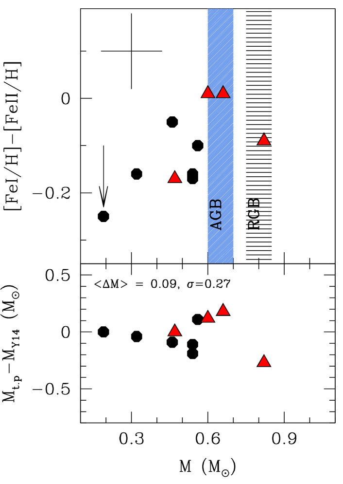
Figure 6: Top panel: the difference [Fe i /H]–[Fe ii /H] (as derived using the hybrid analysis of Section 3) is plotted against the stellar masses inferred from Y14 analysis. The shaded and blue regions define the mass range expected for RGB and AGB stars, respectively.The arrow indicates NR 60, a likely AGB star according to its position in the CMD (see Section 2). The typical error is also plotted in the right upper corner. Symbols are as in Figure 1. Bottom panel: we plot the difference in mass we obtain when stellar masses are estimated using our spectroscopic and Y14 parameters; M_t.p and M_Y14 respectively.

4.1 Stellar masses inferred from spectroscopic gravities

While the [Fe i/H] and [Fe ii/H] distributions are only to some degree changed by the choice of different methods to constrain T_eff, the choice of spectroscopic gravities can heavily affect the measured abundances and hence the conclusions about the degree of homogeneity of the cluster (see Figure 2).

Different methods to derived $\log g$, i.e. photometry, ionisation balance or pressure-broadened wings of strong lines, can provide conflicting results (see e.g. Edvardsson, 1988; Gratton, Carretta & Castelli, 1996; Fuhrmann, 1998; Allende Prieto et al., 1999).

A simple but sound method to check the validity of the spectroscopic gravities is to derive the stellar masses that these gravities imply. In the case of globular cluster stars, where ages and distances are known and are the same for all the stars in a given clusters, the RGB stars will cover a small range of masses and they are expected to have masses larger than 0.5 M_⊙, corresponding to the mass of the He-core for low-mass stars. We estimate stellar masses as inferred from spectroscopic gravities for stars with [Fe/H]$\simeq$–1.5 dex; i.e. the metal-poor and metal-intermediate components in Y14 analysis. We compute stellar masses from the Stefan-Boltzmann equation, starting from the surface gravity values constrained with method (1) in Section 3. We note that the results do not change when using the spectroscopic gravities listed in Y14, being the average difference between our and Y14 mass estimates $\Delta$ M=0.09 M_☉ (see bottom panel in Figure 6, where the inferred stellar masses are compared to each other).

The estimated masses are plotted against the difference in [Fe i/H]–[Fe ii/H] from method (3) in the top panel of Figure 6. Firstly, we note that stars for which [Fe i/H] and [Fe ii/H] lines give the same iron abundance, i.e. stars with [Fe i/H]–[Fe ii/H]$\simeq$ 0, have an estimated mass compatible to that expected for a giant star in a GC (M$\simeq$0.75-0.85 M_☉). Those stars –NR 47 and NR 77– are also the stars for which the ionisation balance gives the same surface gravities along the mean RGB as photometry, and they are also the most metal-rich stars of the canonical RGB according to Y14 analysis (with [Fe/H]=–1.42 and –1.46 dex).

Figure 6 also illustrates how the estimated spectroscopic stellar masses show a very large spread which is not expected for stars in the same evolutionary stage. Indeed, the derived masses range from 0.19 M☉ for NR 60 (a very unlikely value for a giant even taking in to account the uncertainties in the mass loss rate) to 0.82 M☉ for NR 81. Stars with very (unphysical) low masses display the largest difference in the [Fe i/H]–[Fe ii/H]. On the contrary, when the [Fe i/H] and [Fe ii/H] abundance ratios are similar, the spectroscopic gravities provide stellar masses that are compatible within the theoretical expectation (Figure 6).

Interestingly, NR 60 –the star showing the largest [Fe i /H]–[Fe ii /H] difference when photometric gravities are adopted, has been classified as an AGB star by Y14 and its position appears to be consistent with that of an AGB also in our own photometry (see Section 2). The discrepancy between iron abundances measured by Fe i and Fe ii lines for AGB GC stars has been extensively reported in literature in the last few years. Indeed, Fe i lines have been found to provide systematically lower abundances in AGBs with respect to RGBs of the same cluster. This behaviour has been observed in M5 (Ivans et al., 2001), 47 Tuc (Lapenna et al., 2014), NGC 3201 (Mucciarelli et al., 2015a), M22 (Mu15) and M62 (Lapenna et al., 2015).

As discussed before, Y14 find that metal-intermediate stars in their analysis are also enriched in their $s$-process element content with respect to metal-poor stars. Unfortunately, $s$-element abundances have been derived from spectral synthesis by Y14 and only spectra for the nine stars observed with SUBARU are publicly available (3 metal-poor and 2 metal-intermediate stars). Therefore, we do not perform any attempt to measure $s$-element abundances. However, we can tentatively assume that $s$-rich stars are still enriched in their $s$-process element content also when [Fe ii/H] abundances from photometric gravities are taken as a reference.

It is conceivable that this can be the case, as in Lardo et al. (2013) we demonstrate that the split RGB of M 2 observed in the $U$, $U-V$ CMD (Lardo et al., 2012), is composed by two groups of stars which differ by $\simeq$0.5 dex in their $s$-process element content. The analysis presented in Lardo et al. (2013) is based on low-resolution spectra, and [Sr ii/Fe] and [Ba ii/Fe] abundances were measured assuming the same metallicity for all stars. Therefore, the observed spread in the absolute abundances for [Ba ii/Fe] and [Sr ii/Fe] is larger than that measured from [Fe i/H] lines ($\simeq$0.2 dex), possibly indicating that $s$-rich stars in Y14 analysis remain $s$-rich also when [Fe ii/H] abundances derived from photometry are used.

Under this assumption, Figure 6 illustrate that the difference between [Fe i/H]–[Fe ii/H] is also correlated with the $s$-process element content, having $s$-rich stars better agreement between [Fe i/H]–[Fe ii/H] than $s$-normal stars (red triangles and black dots, respectively). In these respects, the main metal-poor component of M 2 is very similar to M 22, where a correlation between the difference between [Fe i/H]–[Fe ii/H] and the $s$-process element content also exists (Mu15).

5 Summary and Conclusions

In this paper we re-derive iron abundances from EW measurements of 14 M 2 RGB stars from which Y14 detect a large metallicity dispersion ($\simeq$ 0.8 dex) with three main components at [Fe/H]$\simeq$–1.7, –1.5, and –1.0 dex. [Fe i/H] and [Fe ii/H] abundances have been calculated using three different approaches to constrain effective temperature and surface gravity. We can summarise our main results as follows:

• We find that the [Fe i/H] and [Fe ii/H] distributions greatly differ when spectroscopic or photometric gravities are adopted in the analysis. In particular, the distribution of [Fe i/H] abundances remains large (and possibly trimodal) irrespective of the choice of spectroscopic or photometric gravities. On the other hand, when photometric gravities are used, the [Fe ii/H] distribution is clearly bimodal, with two separate components at [Fe/H]$\simeq$–1.5 and –1.1 dex. Both stellar groups are compatible with no internal iron spread.

  Hence, the large majority of cluster’s stars, i.e. $\simeq$ 99% of the total cluster population, do not show any evidence for a metallicity spread. Stars in this metallicity group show the C-N, Na-O anti-correlations typical of GCs, as well as a bimodality in their $s$-process content (Lardo et al., 2012, 2013, Y14) which is somewhat connected to the observed discrepancy between Fe i and Fe ii abundances (see Setion 4.1). On the contrary, we confirm the presence of a second metallicity component (Yong et al., 2014b). Stars at [Fe ii/H] $\simeq$ –1.1 dex, if members, represent a very small fraction of M 2 stars, accounting only for $\sim$1% of the cluster population (Milone et al., 2015).

• The results presented in this paper for the metal-poor stars in M 2 are similar to what found by Mu15 in M 22. The absence of a metallicity spread among M 22 stars claimed by Mu15 (but see Da Costa et al., 2009, and Marino et al., 2011) would rule out the hypothesis that the cluster was significantly more massive in the past and possibly the remnant of a now disrupted dwarf galaxy (see Bastian & Lardo, 2015, for a discussion on the mass loss problem in GCs). We stress, however, that our study confirms the presence of a second minority population with different iron abundance with respect to the bulk of M 2 stars (Yong et al., 2014b). This additional metal-rich population appears not to be present in M 22 (Mu15; but see Da Costa et al., 2009, and Marino et al., 2011).

• Fe i lines are commonly used to derive iron abundances, because a considerable number of Fe i lines in a rather large range of EP with accurate transition probabilities exists (e.g. Blackwell, Petford & Shallis, 1979). However, even if accurate laboratory atomic data are available for a limited number of Fe ii lines (see Appendix A2 of Lambert et al., 1996, for an extensive investigation of the reliability of $\log g_{f}$ values for Fe ii); in the atmospheres of giant stars iron is almost completely ionised (Kraft & Ivans, 2003) and Fe ii lines do not suffer for departure from LTE, at variance with Fe i ones. As a result, metallicity is more safely derived from the dominant species, Fe ii, than from Fe i.

  We consistently used the same Fe ii data for all the programme stars. Therefore, the uncertainty in the Fe ii $\log g_{f}$ values is expected to touch only the zero-point (i.e. the absolute value) of the [Fe ii/H] abundances, while leaving the [Fe ii/H] distribution of the entire stellar sample unaffected. Indeed, the [Fe ii/H] distribution is bimodal even when considering different sources for the atomic data (e.g., Meléndez & Cohen, 2009; Raassen & Uylings, 1998; see Figure 5).

  The same number of Fe ii lines ($\simeq$10-20) used in this paper to infer metallicities has been used by Y14 to derive atmospheric parameters; and the atmospheric parameters derived in such fashion would not be considered as unreliable due to the small number of lines of Fe ii used to constrain gravity.

• From a qualitative point of view, the (negative) difference between [Fe i/H] and [Fe ii /H] observed in some M 2 stars is consistent with the occurrence of NLTE effects driven by overionisation, as the most metal-poor stars in the [Fe i/H] distribution are shifted to higher metallicities in the [Fe ii/H] distribution. The same holds also for different choices of literature sources for the $\log g_{f}$ (e.g., Meléndez & Cohen, 2009; Raassen & Uylings, 1998).

  In the atmospheres of metal-poor giants, Fe ii is the dominant species throughout the atmosphere, so that NLTE effects are negligible for Fe ii, while they are extremely important for Fe i. For example, Thévenin & Idiart (1999) find that the reduction of [Fe/H] estimated from Fe i relative to Fe ii amounts to about 0.1 dex at [Fe/H] = –1 dex and about 0.3 dex at [Fe/H] = –2.5 dex (see also Lambert et al., 1996).

  However, the observed differences are not quantitative compatible with the theoretical predictions (e.g. Bergemann et al., 2012), suggesting that this interpretation is no correct or that the available NLTE correction grids are not suitable for these stars.

The observational evidence collected in the last years provide a more complex picture for the so-called anomalous clusters, not easy to interpret from a theoretical point of view. Observationally, we note that there are two circumstances where the use of spectroscopic gravities leads to spurious iron spreads:

1. In normal clusters, i.e. clusters showing only the characteristic Na-O anticorrelation, the detection of a spurious iron spread can be ascribed to the inclusion of AGB stars in the spectroscopic sample, i.e. Mucciarelli et al. (2015a). When AGB stars are removed from the analysis, such clusters show no evidence for a significant iron spread. This remains true when both photometric and spectroscopic gravities are adopted. Therefore, it appears not so surprising that normal clusters result to be mono-metallic also when analysed with spectroscopic gravities, if the sample include only RGB stars. For example, Mu15 compared M 22 stellar metallicities with those of NGC 6752, using the same analysis method. They found no evidence for a significant iron spread among NGC 6752 stars also when atmospheric parameters are derived in a classical spectroscopic fashion. Finally, we note that the largest study surveying GC stars, i.e. the Na-O anticorrelation and HB project (see e.g. Carretta et al., 2009a, b), carefully avoids to target AGB stars.

2. In anomalous clusters; i.e. clusters with spreads in $s$-process elements (and possibly C+N+O), double SGB and split RGB (as in the case of M22 and the the majority of M2, see Introduction) a spurious spread is derived when spectroscopic gravities are adopted. Such clusters are indeed mono-metallic when Fe ii lines and photometric gravities are used in the analysis. Again, the group publishing the largest metallicity database for GC stars, i.e. the Na-O anticorrelation and HB project, consistently use photometric data to constrain both effective temperatures and surface gravities. This explains why clusters showing intrinsic [Fe/H] are relatively rare. For example, Yong et al. (2014a) performed the same analysis as on M 2 stars in M 62, finding no evidence for iron dispersion. This cluster is the ninth most luminous cluster in the Galaxy and it is characterised by an extended horizontal branch, yet it does show neither a $s$-process element bimodality (Yong et al., 2014a) nor a photometric SGB split. Similarly, Carretta et al. (2013) did not report a metallicity spread for stars in NGC 362, an anomalous cluster with mass comparable to that of M 22, which shows a split SGB, a multimodal RGB, and a spread in its $s$-process element content. To constrain atmospheric parameters, Carretta et al. (2013) followed the same procedure adopted for the other GCs targeted by their FLAMES survey, i.e. photometric stellar gravities.

   All the above is consistent with our hypothesis that spectroscopic gravities yield artificial iron spreads only in anomalous clusters, a relatively small subset of the Milky Way GC population.

So far, a number of GCs have been claimed to host different populations of stars with different metallicities. Large iron distributions have been found in $\omega$ Centauri (Johnson & Pilachowski, 2010, e.g.), M 54 (Carretta et al., 2010a), and Terzan 5 (e.g. Massari et al., 2014). Additionally, smaller intrinsic spreads, i.e. comparable to those found by Marino et al. (2009) and Y14 in the case of M 22 and the main metal-poor component in M 2, are found in a growing number of GCs. The analysis presented in Mu15 and in this paper casts doubt upon the presence of these intrinsic spreads, which can have been artificially produced by the choices to constrain atmospheric parameters. In particular, the use of spectroscopic gravities in both M 22 (Mu15) and M 2 leads to very low stellar masses which are unphysical for a giant star. Our findings suggest caution when analysing metal-poor stars using gravities obtained from the ionisation balance, and indicates the need to carefully reanalyse clusters found to display an intrinsic iron spread (e.g. M 19, NGC 5286).

6 acknowledgements

We thank E. Pancino, M. Bellazzini, G. Altavilla, G. Cocozza, S. Marinoni, S. Ragainini for providing photometry. NB gratefully acknowledges funding from the Royal Society and European Research Council (grant 646928 ”Multi-Pop”). This research is also part of the project COSMIC-LAB (http://www.cosmic-lab.eu) funded by the European Research Council (under contract ERC-2010-AdG-267675).

Table 3: Fe ii atomic data and EWs presented by Yong et al. (2014b) for the program stars.

Lambda	E.P.	$\log gf$	NR 37	NR 38	NR 47	NR 58	NR 60	NR 76	NR 77	NR 81	NR 99	NR 124	NR 132	NR 207	NR 254	NR 378
Å	eV		mÅ	mÅ	mÅ	mÅ	mÅ	mÅ	mÅ	mÅ	mÅ	mÅ	mÅ	mÅ	mÅ	mÅ
4128.75	2.58	$-$3.47	…	…	…	58.6 (1)	51.9 (1)	…	…	…	…	…	…	…	…	…
4178.86	2.58	$-$2.53	…	…	…	80.1 (1)	114.6 (-1)	…	…	…	…	…	…	…	…	…
4416.82	2.78	$-$2.43	92.8 (1)	…	…	95.9 (1)	115.5 (-1)	88.1 (-1)	110.3 (1)	105.4 (1)	…	…	116.7 (-1)	…	…	…
4491.40	2.86	$-$2.60	75.9 (1)	67.8 (1)	…	71.6 (1)	92.6 (1)	…	…	75.3 (1)	…	…	75.3 (-1)	…	…	…
4508.29	2.85	$-$2.31	…	…	…	…	…	85.8 (-1)	…	82.5 (1)	91.4 (1)	103.0 (1)	89.9 (-1)	…	95.8 (-1)	108.2 (-1)
4508.30	2.86	$-$2.28	…	…	…	91.5 (1)	…	…	…	…	…	…	…	…	…	…
4541.52	2.86	$-$2.81	62.7 (1)	…	…	…	89.0 (1)	62.4 (1)	…	…	…	…	89.2 (-1)	…	…	…
4555.89	2.83	$-$2.18	…	…	…	…	…	92.9 (-1)	…	…	…	…	…	…	…	…
4576.34	2.84	$-$2.90	68.1 (1)	90.5 (1)	…	72.7 (1)	79.5 (1)	62.5 (1)	84.3 (1)	…	…	75.0 (1)	90.2 (-1)	…	…	85.7 (1)
4582.84	2.84	$-$3.09	…	…	…	…	74.5 (1)	57.0 (1)	…	48.3 (1)	…	…	…	…	…	…
4620.52	2.83	$-$3.20	47.6 (1)	58.7 (1)	44.4 (1)	46.7 (1)	59.6 (1)	45.5 (1)	42.8 (1)	49.4 (1)	48.6 (1)	61.8 (1)	57.6 (1)	…	…	69.8 (1)
4833.19	2.66	$-$4.62	15.6 (1)	…	…	…	…	…	…	11.0 (-1)	…	…	…	…	…	…
4840.00	2.68	$-$4.74	…	…	…	…	…	…	22.2 (1)	…	…	…	…	…	…	…
4893.82	2.83	$-$4.29	…	…	…	20.1 (1)	19.6 (1)	16.2 (1)	…	…	…	…	…	…	…	…
4993.36	2.81	$-$3.48	…	…	40.4 (1)	…	49.7 (1)	32.4 (1)	…	37.7 (1)	…	35.0 (1)	50.9 (1)	40.6 (1)	46.0 (1)	…
5100.66	2.81	$-$4.16	15.3 (-1)	…	…	12.9 (-1)	15.1 (-1)	16.5 (1)	…	17.7 (-1)	…	…	30.7 (1)	…	…	…
5132.67	2.81	$-$3.95	18.1 (1)	…	…	…	20.9 (1)	14.8 (-1)	…	14.9 (-1)	16.4 (1)	…	33.4 (1)	…	…	…
5197.58	3.23	$-$2.23	78.6 (1)	83.9 (1)	…	79.9 (1)	98.8 (1)	77.7 (1)	…	87.4 (1)	…	…	96.4 (-1)	…	…	…
5234.63	3.22	$-$2.22	78.7 (1)	78.0 (1)	…	77.8 (1)	93.3 (1)	83.4 (-1)	…	70.7 (1)	86.8 (1)	…	88.3 (-1)	81.0 (1)	87.8 (1)	105.2 (-1)
5264.81	3.34	$-$3.21	40.2 (1)	39.8 (1)	33.1 (1)	38.5 (1)	43.6 (1)	34.2 (1)	…	30.2 (1)	…	45.6 (1)	42.9 (1)	47.2 (1)	51.9 ( 0)	…
5284.11	2.89	$-$3.01	…	…	…	…	…	51.2 (1)	…	55.2 (1)	…	62.8 (1)	65.1 (1)	…	…	…
5325.56	3.22	$-$3.18	28.7 (1)	39.3 (1)	…	40.4 (1)	…	32.6 (1)	…	37.4 (1)	…	43.0 (1)	41.1 (1)	43.8 (1)	…	…
5414.08	3.22	$-$3.61	…	…	…	…	18.4 (1)	…	…	…	…	…	…	…	…	…
5425.26	3.20	$-$3.27	26.9 (1)	29.7 (1)	31.1 (1)	28.7 (1)	33.3 (1)	32.0 (1)	…	34.4 (1)	31.7 (1)	28.4 (1)	45.7 (1)	36.9 (1)	36.2 (1 )	…
5525.13	3.27	$-$4.00	…	…	…	…	13.8 (-1)	…	…	…	…	…	…	…	…	…
5534.85	3.25	$-$2.75	52.3 (1)	56.0 (1)	…	53.9 (1)	60.5 (1)	48.3 (1)	…	50.8 (1)	…	57.5 (1)	…	…	…	…
5991.38	3.15	$-$3.56	25.7 (1)	21.9 (1)	23.4 (1)	19.0 (1)	26.1 (1)	27.6 (1)	…	25.7 (1)	22.8 (1)	23.4 (1)	38.5 (1)	28.0 (1)	29.8 (1)	39.9 (1)
6084.11	3.20	$-$3.81	13.7 (-1)	15.0 (-1)	…	13.8 (-1)	…	13.0 (-1)	…	15.9 (-1)	…	…	20.1 (1)	18.9 (-1)	…	26.1 (1)
6113.33	3.22	$-$4.13	…	…	…	…	13.1 (-1)	…	14.6 (-1)	15.4 (-1)	…	…	16.8 (-1)	…	…	…
6149.25	3.89	$-$2.73	20.8 (1)	…	…	18.7 (-1)	…	24.3 (1)	…	21.1 (-1)	20.6 (1)	22.9 (1)	28.0 (1)	…	…	39.9 (1)
6247.56	3.89	$-$2.33	34.5 (1)	31.2 (1)	28.2 (1)	37.4 (1)	42.0 (1)	32.4 (1)	40.0 (1)	30.5 (1)	40.0 (1)	37.0 (1)	36.7 (1)	…	44.5 (1)	54.9 (1)
6369.46	2.89	$-$4.21	12.8 (-1)	12.4 (-1)	…	16.7 (-1)	15.6 (-1)	16.6 (-1)	…	11.2 (-1)	…	…	20.0 (-1)	16.8 (-1)	23.2 (1)	…
6416.93	3.89	$-$2.70	…	…	…	21.3 (1)	…	15.7 (-1)	…	…	…	…	…	…	32.1 (1)	…
6432.68	2.89	$-$3.58	31.0 (1)	34.8 (1)	29.3 (1)	34.7 (1)	38.3 (1)	33.7 (1)	31.0 (1)	29.4 (1)	34.7 (1)	33.2 (1)	38.0 (1)	39.4 (1)	49.0 (1)	53.6 (1)
6456.39	3.90	$-$2.10	46.1 (1)	44.1 (1)	35.0 (1)	…	…	…	48.5 (1)	46.8 (1)	45.8 (1)	…	55.8 (1)	51.2 (1)	57.3 (1)	…
6516.08	2.89	$-$3.38	49.0 (1)	46.9 (1)	…	58.4 (1)	56.5 (1)	51.7 (1)	…	…	50.7 (1)	49.1 (1)	…	…	59.0 (1)	…
7711.72	3.90	$-$2.54	24.1 (-1)	25.7 (1)	…	21.9 (-1)	28.3 (1)	…	35.0 (1)	…	…	…	…	…	…	…

References

- Allende Prieto et al. (1999) Allende Prieto C., García López R. J., Lambert D. L., Gustafsson B., 1999, ApJ, 527, 879
- Alonso, Arribas & Martínez-Roger (1999) Alonso A., Arribas S., Martínez-Roger C., 1999, A&AS, 140, 261
- Bastian & Lardo (2015) Bastian N., Lardo C., 2015, MNRAS, 453, 357
- Baumgardt, Kroupa & Parmentier (2008) Baumgardt H., Kroupa P., Parmentier G., 2008, MNRAS, 384, 1231
- Bergbusch & VandenBerg (2001) Bergbusch P. A., VandenBerg D. A., 2001, ApJ, 556, 322
- Bergemann et al. (2012) Bergemann M., Lind K., Collet R., Magic Z., Asplund M., 2012, MNRAS, 427, 27
- Bernstein et al. (2003) Bernstein R., Shectman S. A., Gunnels S. M., Mochnacki S., Athey A. E., 2003, in Society of Photo-Optical Instrumentation Engineers (SPIE) Conference Series, Vol. 4841, Instrument Design and Performance for Optical/Infrared Ground-based Telescopes, Iye M., Moorwood A. F. M., eds., pp. 1694–1704
- Biemont et al. (1991) Biemont E., Baudoux M., Kurucz R. L., Ansbacher W., Pinnington E. H., 1991, A&A, 249, 539
- Blackwell et al. (1986) Blackwell D. E., Booth A. J., Haddock D. J., Petford A. D., Leggett S. K., 1986, MNRAS, 220, 549
- Blackwell et al. (1979) Blackwell D. E., Ibbetson P. A., Petford A. D., Shallis M. J., 1979, MNRAS, 186, 633
- Blackwell, Lynas-Gray & Smith (1995) Blackwell D. E., Lynas-Gray A. E., Smith G., 1995, A&A, 296, 217
- Blackwell, Petford & Shallis (1979) Blackwell D. E., Petford A. D., Shallis M. J., 1979, MNRAS, 186, 657
- Blackwell et al. (1980) Blackwell D. E., Petford A. D., Shallis M. J., Simmons G. J., 1980, MNRAS, 191, 445
- Carretta et al. (2009a) Carretta E., Bragaglia A., Gratton R., Lucatello S., 2009a, A&A, 505, 139
- Carretta et al. (2010a) Carretta E. et al., 2010a, A&A, 520, A95
- Carretta et al. (2009b) Carretta E. et al., 2009b, A&A, 505, 117
- Carretta et al. (2013) Carretta E. et al., 2013, A&A, 557, A138
- Carretta et al. (2010b) Carretta E. et al., 2010b, ApJL, 722, L1
- Castelli & Kurucz (2003) Castelli F., Kurucz R. L., 2003, in IAU Symposium, Vol. 210, Modelling of Stellar Atmospheres, Piskunov N., Weiss W. W., Gray D. F., eds., p. 20P
- Cayrel et al. (2004) Cayrel R. et al., 2004, A&A, 416, 1117
- Cudworth & Rauscher (1987) Cudworth K. M., Rauscher B. J., 1987, AJ, 93, 856
- Da Costa et al. (2009) Da Costa G. S., Held E. V., Saviane I., Gullieuszik M., 2009, ApJ, 705, 1481
- Edvardsson (1988) Edvardsson B., 1988, A&A, 190, 148
- Fabrizio et al. (2012) Fabrizio M. et al., 2012, PASP, 124, 519
- Fuhrmann (1998) Fuhrmann K., 1998, A&A, 330, 626
- Gratton, Sneden & Carretta (2004) Gratton R., Sneden C., Carretta E., 2004, araa, 42, 385
- Gratton, Carretta & Bragaglia (2012) Gratton R. G., Carretta E., Bragaglia A., 2012, A&ARv, 20, 50
- Gratton, Carretta & Castelli (1996) Gratton R. G., Carretta E., Castelli F., 1996, A&A, 314, 191
- Gratton et al. (2003) Gratton R. G., Carretta E., Claudi R., Lucatello S., Barbieri M., 2003, A&A, 404, 187
- Grevesse & Sauval (1998) Grevesse N., Sauval A. J., 1998, ssr, 85, 161
- Grundahl et al. (1999) Grundahl F., Catelan M., Landsman W. B., Stetson P. B., Andersen M. I., 1999, ApJ, 524, 242
- Harris (1996) Harris W. E., 1996, AJ, 112, 1487
- Ivans et al. (2001) Ivans I. I., Kraft R. P., Sneden C., Smith G. H., Rich R. M., Shetrone M., 2001, AJ, 122, 1438
- Johnson & Pilachowski (2010) Johnson C. I., Pilachowski C. A., 2010, ApJ, 722, 1373
- Johnson et al. (2015) Johnson C. I., Rich R. M., Pilachowski C. A., Caldwell N., Mateo M., Bailey, III J. I., Crane J. D., 2015, AJ, 150, 63
- Kraft (1994) Kraft R. P., 1994, PASP, 106, 553
- Kraft & Ivans (2003) Kraft R. P., Ivans I. I., 2003, PASP, 115, 143
- Lambert et al. (1996) Lambert D. L., Heath J. E., Lemke M., Drake J., 1996, ApJS, 103, 183
- Lapenna et al. (2015) Lapenna E., Mucciarelli A., Ferraro F. R., Origlia L., Lanzoni B., Massari D., Dalessandro E., 2015, ApJ, 813, 97
- Lapenna et al. (2014) Lapenna E., Mucciarelli A., Lanzoni B., Ferraro F. R., Dalessandro E., Origlia L., Massari D., 2014, ApJ, 797, 124
- Lardo et al. (2013) Lardo C. et al., 2013, MNRAS, 433, 1941
- Lardo et al. (2012) Lardo C., Pancino E., Mucciarelli A., Milone A. P., 2012, A&A, 548, A107
- Marino et al. (2015) Marino A. F. et al., 2015, ArXiv e-prints
- Marino et al. (2009) Marino A. F., Milone A. P., Piotto G., Villanova S., Bedin L. R., Bellini A., Renzini A., 2009, A&A, 505, 1099
- Marino et al. (2012) Marino A. F. et al., 2012, A&A, 541, A15
- Marino et al. (2011) Marino A. F. et al., 2011, A&A, 532, A8
- Mashonkina et al. (2011) Mashonkina L., Gehren T., Shi J.-R., Korn A. J., Grupp F., 2011, A&A, 528, A87
- Massari et al. (2014) Massari D. et al., 2014, ApJ, 795, 22
- Meléndez & Cohen (2009) Meléndez J., Cohen J. G., 2009, ApJ, 699, 2017
- Milone et al. (2008) Milone A. P. et al., 2008, ApJ, 673, 241
- Milone et al. (2015) Milone A. P. et al., 2015, MNRAS, 447, 927
- Mucciarelli et al. (2015a) Mucciarelli A., Lapenna E., Massari D., Ferraro F. R., Lanzoni B., 2015a, ApJ, 801, 69
- Mucciarelli et al. (2015b) Mucciarelli A., Lapenna E., Massari D., Pancino E., Stetson P. B., Ferraro F. R., Lanzoni B., Lardo C., 2015b, ApJ, 809, 128
- Mucciarelli et al. (2013) Mucciarelli A., Pancino E., Lovisi L., Ferraro F. R., Lapenna E., 2013, ApJ, 766, 78
- Noguchi et al. (2002) Noguchi K. et al., 2002, PASJ, 54, 855
- Pancino & Gaia-ESO Survey consortium (2012) Pancino E., Gaia-ESO Survey consortium o. b. o. t., 2012, ArXiv e-prints
- Pfeffer et al. (2014) Pfeffer J., Griffen B. F., Baumgardt H., Hilker M., 2014, MNRAS, 444, 3670
- Pietrinferni et al. (2004) Pietrinferni A., Cassisi S., Salaris M., Castelli F., 2004, ApJ, 612, 168
- Pietrinferni et al. (2006) Pietrinferni A., Cassisi S., Salaris M., Castelli F., 2006, ApJ, 642, 797
- Piotto (2009) Piotto G., 2009, in IAU Symposium, Vol. 258, IAU Symposium, E. E. MamAJek, D. R. Soderblom, & R. F. G. Wyse, ed., pp. 233–244
- Piotto et al. (2012) Piotto G. et al., 2012, ApJ, 760, 39
- Raassen & Uylings (1998) Raassen A. J. J., Uylings P. H. M., 1998, A&A, 340, 300
- Sarajedini et al. (2007) Sarajedini A. et al., 2007, AJ, 133, 1658
- Stetson (1987) Stetson P. B., 1987, PASP, 99, 191
- Stetson (1992) Stetson P. B., 1992, in Astronomical Society of the Pacific Conference Series, Vol. 25, Astronomical Data Analysis Software and Systems I, Worrall D. M., Biemesderfer C., Barnes J., eds., p. 297
- Thévenin & Idiart (1999) Thévenin F., Idiart T. P., 1999, ApJ, 521, 753
- Valdes (1998) Valdes F. G., 1998, in Astronomical Society of the Pacific Conference Series, Vol. 145, Astronomical Data Analysis Software and Systems VII, Albrecht R., Hook R. N., Bushouse H. A., eds., p. 53
- Villanova, Geisler & Piotto (2010) Villanova S., Geisler D., Piotto G., 2010, ApJL, 722, L18
- Yong et al. (2014a) Yong D. et al., 2014a, MNRAS, 439, 2638
- Yong & Grundahl (2008) Yong D., Grundahl F., 2008, ApJL, 672, L29
- Yong et al. (2014b) Yong D. et al., 2014b, MNRAS, 441, 3396