Chirality and Current-Current Correlation in Fractional Quantum Hall Systems.

Abstract

We study current-current correlation in an electronic analog of a beam splitter realized with edge channels of a fractional quantum Hall liquid at Laughlin filling fractions. In analogy with the known result for chiral electronsBüttiker (1992), if the currents are measured at points located after the beam splitter, we find that the zero frequency equilibrium correlation vanishes due to the chiral propagation along the edge channels. Furthermore, we show that the current-current correlation, normalized to the tunneling current, exhibits clear signatures of the Laughlin quasi-particles’ fractional statistics.

I Introduction

With the theoretical explanation of the Fractional Quantum Hall (FQH) effect at filling $\nu=1/m$, with $m$ odd Tsui et al. (1982), Laughlin made the remarkable prediction that the elementary charged excitation of a FQH system is a quasiparticle carrying fractional charge $q=\nu e$. Laughlin (1983) Moreover, Laughlin’s quasiparticles (LQP) were predicted to carry fractional statistics, as well, that is, on exchanging two of them with each other, the relative wavefunction must acquire a statistical phase $\theta\neq\{\pi,2\pi\}$, with $\theta=\pi$ corresponding to fermions, $\theta=2\pi$ corresponding to bosons. As a result, they behave as Abelian anyons with fractional charge $q$.Arovas et al. (1984)

Even richer structures are possible in the case of non-Abelian anyons—the braiding of one quasi-particle by another one will result in the system to be sent into a different quantum state and not only in the relative wavefunction to acquire a statistical phaseNayak et al. (2008).

A FQH system is fully gapped in the bulk, with gapless branches of chiral excitations at its edges, supporting current flow across the sample. The elementary charge carrier is the boundary analog of a LQP and, therefore, it carries a fractional charge $q$, as well Wen (2004). Because of such a correspondence, it was possible to experimentally estabilish the fractional charge of LQPs by means of shot-noise measurements on a FQH-bar de Picciotto et al. (1997); Saminadayar et al. (1997). Nevertheless, a direct observation of their fractional statistics is still the subject of ongoing experimental effortsCamino et al. (2005); Willett et al. (2013).

Correlation measurements of light intensities in opticsHanbury Brown and Twiss (1954, 1956) and electrical currents in solid-state physicsOliver et al. (1999) have provided an important tool to investigate the difference between the two ”classical” statistics of quantum elementary particles: bosonic and fermionic. In the pursue of evidence for fractional statistics in FQH systems, a number of works have been putting forward the use of solid-state analogs of Fabry-Perotde C. Chamon et al. (1997); Stern and Halperin (2006); Bonderson et al. (2006a, b); Ardonne and Kim (2008); Bishara et al. (2009); Halperin et al. (2011), Mach-ZehnderLaw et al. (2006); Feldman et al. (2007); Ponomarenko and Averin (2007, 2009); Bonderson et al. (2008); Law (2008); Levkivskyi et al. (2009); Ponomarenko and Averin (2010); Wang and Feldman (2010); Levkivskyi et al. (2012); Ganeshan et al. (2012); Yang (2015) and more elaborated Hanbury Brown and Twiss Safi et al. (2001); Vishveshwara (2003); Kim et al. (2005, 2006); Campagnano et al. (2012, 2013) interferometers to address the statistical properties of fractional quantum Hall anyons.

In this Article we confine our attention to Abelian anyons, emerging as elementary charged excitations of a FQH-state at a Laughlin filling $\nu$. We focus on a simple measurement with LQPs colliding at a beam splitter-like device, such an experiment is not subject to some of the intricacies found in interferometric setups. In order to illustrate our approach, we start by considering a simple, but instructive, example. With reference to Fig. 1, we consider a beam splitter where particles are injected from sources $S_{1}$ and $S_{2}$ and measured at detectors $D_{1}$ and $D_{2}$. An incoming particle from $S_{1}$ can be either transmitted to $D_{2}$ with scattering amplitude $t$, or reflected to $D_{1}$ with scattering amplitude $r$ . Similarly an incoming particle from $S_{2}$ can be either transmitted to $D_{1}$ with scattering amplitude $t^{\prime}$, or reflected to $D_{2}$ with scattering amplitude $r^{\prime}$, so that the scattering matrix describing these processes is given by

$$S=\left(\begin{array}[]{cc}r&t^{\prime}\\ t&r^{\prime}\end{array}\right)\,.$$ (1)

Because of the particle number conservation, $S$ must be unitary, which enables us to use the following parametrization

$$S=\left(\begin{array}[]{cc}\sqrt{\mathcal{R}}&\sqrt{\mathcal{T}}\\ \sqrt{\mathcal{T}}&-\sqrt{\mathcal{R}}\end{array}\right)\,,$$ (2)

with $\mathcal{T}$ and $\mathcal{R}$ respectively being the transmission and reflection coefficients. Let $n_{D_{1}}$ and $n_{D_{2}}$ respectively be the particle number operators at $D_{1}$ and at $D_{2}$. Let us assume that the particles considered are either fermions, or bosons.

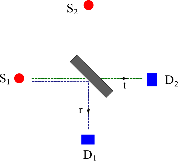
Figure 1: In Figure we represent a scheme of a beam splitter. Particles emitted from source $S_{1}$ can be transmitted to detector $D_{2}$ with transmission amplitude $t$ or reflected to detector $D_{2}$ with amplitude $r$. Similarly for particles emitted from source $S_{2}$ (these processes are not illustrated in Figure). For photons, which obey Bose-Einstein statistics, the physical realisation of a beam splitter is a partially silvered mirror. In the case of electrons, which obey Fermi-Dirac statistics, a beam splitter can be realized using edges of an integer quantum Hall liquid impinging on a quantum point contact.

Following Ref.[Blanter and Buettiker, 2000], and considering a toy model with just one quantum mode per arm, one can calculate the correlation between the number of particles measured at $D_{1}$ and at $D_{2}$, i.e. $\langle\langle n_{D_{1}}n_{D_{2}}\rangle\rangle=\langle n_{D_{1}}n_{D_{2}}\rangle-\langle n_{D_{1}}\rangle\langle n_{D_{2}}\rangle$. Notwithstanding that in optics very special incoming states can be realized, in a typical experiments, such as in transport measurements in solid-state physics—the appropriate tool to investigate Abelian anyons at a FQH-edge—particles colliding at a beam splitter emerge from thermal reservoirs.

Assuming that the particles are emitted from two independent reservoirs $S_{1}$ and $S_{2}$, respectively characterised by (thermal) distribution functions $n_{1}$ and $n_{2}$, one obtains

$$\langle\langle n_{D_{1}}n_{D_{2}}\rangle\rangle=\pm\mathcal{RT}(n_{1}-n_{2})^{2},$$ (3)

where the plus and minus sign refer to bosons and fermions respectively. It is worth stressing that, as it is apparent from Eq.(3), when $n_{1}=n_{2}$, the correlations vanish, irrespectively of the underlying quantum statistics Büttiker (1991). In this article we derive the analog of Eq.(3) for LQPs originating from sources (FQH edges) kept at the same temperature but, in general, at different chemical potentials. For FQH anyons there is no simple description of the beam splitter in terms of a scattering matrix. Therefore, we perform the calculation by resorting to non-equilibrium Keldysh formalism. In particular, we realize the beam splitter as a quantum point contact (QPC) which allows for LQP tunneling between the edges. Besides weak inter-edge tunneling, no other approximation is involved in our calculation. As a result, while in the ”shot-noise” regime, $|eV|\gg k_{B}T$ ($V$ being the voltage bias between the edges and $k_{B}$ being the Boltzmann constant) we recover that correlations are proportional to the tunneling current, with the constant of proportionality being equal to $q$, in the ”thermal” regime $|eV|\ll k_{B}T$ the constant of proportionality is renormalized by a purely statistics dependent function $\gamma(\nu)=(6/\pi^{2})\partial_{z}^{2}\ln\Gamma(z)\big{|}_{z=\nu}$ [$\Gamma(z)$ being Euler Gamma function], which can be directly measured by looking at current-current correlation probed in the appropriate regime.

The Article is organized as follows: In Section II we introduce the model for a beam splitter realized with edge channels of a FQH system; In Section III, we calculate the correlation of currents measured at different drains as a function of the voltage bias V and the temperature $T$. In Section IV we show how fractional statistics can be probed from current-current correlation normalized to the tunneling current. In Section V we discuss and summarize our results and give an outlook of the possible implications of our work. Mathematical details and a review of the non-interacting case ($\nu=1$) are provided in the appendices.

II The Model

In this Section we introduce the model for the edge channels that we use in the calculation of the current-current correlation.

Throughout this Article, we limit our analysis to Laughlin’s states at filling $\nu$, which are characterized by only one branch of chiral excitations per edge Wen (2004). This is not a potential limitations, as we outline in the concluding Section. Our analysis, indeed, is expected to be generalizable to non-Laughlin FQH states, e.g. $\nu=2/3$ and $\nu=5/2$, as a possible tool to investigate the properties of these more exotic FHQ states.

The device we discuss here has four edge channels (cfr. Fig. 2), we only need to focus onto the ones labelled $e_{1}$ and $e_{2}$. In order to realize a beam splitter, we assume that a QPC is obtained between the two channels by means of electric gates, allowing for quasiparticle tunneling between $e_{1}$ and $e_{2}$. Finally, it is worth stressing that we choose our geometry to allow for independent tuning of the chemical potentials at $e_{1}$ and $e_{2}$, respectively $\mu_{1}$ and $\mu_{2}$.

Edge excitations of Laughlin’s FQH states are described within chiral Luttinger liquid (CLL)-framework Wen (2004). In the two-edge model, the Hamiltonian for the edges is given by

$$H_{0}=\frac{\hbar v}{4\pi}\sum_{k=1,2}\int dx(\partial_{x}\phi_{k}(x))^{2}\>\>\>\>,$$ (4)

with $v$ the plasmonic velocity. The chiral bosonic fields $\{\phi_{1}(x),\phi_{2}(x)\}$ obey the commutation relations

$$[\phi_{k}(x),\phi_{l}(x^{\prime})]=i\pi\delta_{k,l}\mbox{sgn}(x-x^{\prime})\>\>\>\>.$$ (5)

With the normalizations in Eqs.(4,5), the density operator at edge-$k$ $(k=1,2)$, $\rho_{k}(x)$ is given by

$$\rho_{k}(x)=-\frac{\sqrt{\nu}}{2\pi}\partial_{x}\phi_{k}(x)\,,$$ (6)

while, because of the chiral propagation along the edges, the electric current density operator is: $i_{k}(x)=ev\rho_{k}(x)$.

The Hamiltonian operator describing tunneling of a charge-$q$ LQP at the QPC is constructed in terms of the quasiparticle creation and annihilation operators at edge-$k$. Within CLL-framework, these are realized in terms of vertex operators, respectively given by

$$V_{k}^{\dagger}(x) = F_{k}^{\dagger}e^{i\sqrt{\nu}\phi_{k}(x)}$$

$$V_{k}(x) = F_{k}e^{-i\sqrt{\nu}\phi_{k}(x)}\>\>\>,$$ (7)

with $\{F_{k},F_{k}^{\dagger}\}$ being Klein factors that one has to introduce, in order to recover the correct commutation relations between operators belonging to different edges. Choosing the $x$-coordinates so that the QPC is located at $x=0$, we take the tunneling Hamiltonian to be

$$H_{T}=\Gamma V^{\dagger}_{1}(0)V_{2}(0)+{\rm h.c.}$$ (8)

We have assumed to work in a temperature/voltage regime such that terms that are less relevant in the renormalization group sense Kane and Fisher (1992, 1994) can be disregarded. These terms, indeed, correspond to tunneling of quasiparticles with charge being an integer multiple of $q$.

In fact, as our device contains only one QPC, Klein factors can be dropped from the tunneling Hamiltonian $H_{T}$. Following Ref.[Guyon et al., 2002], the commutation rules between Klein factors must be assigned so that vertex operators corresponding to different edges must obey the same commutation relations as vertex operators corresponding to the same edge, that is, $e^{i\sqrt{\nu}\phi_{k}(x_{1})}e^{i\sqrt{\nu}\phi_{k^{\prime}}(x_{2})}=e^{i\pi\nu{\rm sgn}(x_{1}-x_{2})}e^{i\sqrt{\nu}\phi_{k^{\prime}}(x_{2})}e^{i\sqrt{\nu}\phi_{k}(x_{1})}$. As a result, they have to satisfy the relations $F_{i}^{\dagger}F_{i}=F_{i}F_{i}^{\dagger}=1$, $F_{1}F_{2}=e^{i\nu\pi}F_{2}F_{1}$, and $F_{1}^{\dagger}F_{2}=e^{-i\nu\pi}F_{2}F_{1}^{\dagger}$. Taking into account these commutation relations, it is easy to check that the commutator between $H_{T}$ in interaction representation computed at different times, that is, $[H_{T}(t_{1}),H_{T}(t_{2})]$ is the same, whether or not one introduces the Klein factors in the vertex operators in Eq.(7). Therefore, they can safely disregarded, without affecting the validity of our derivation. The tunneling Hamiltonian $H_{T}$ can be simplified to

$$H_{T}=\Gamma e^{i\sqrt{\nu}(\phi_{1}(0)-\phi_{2}(0))}+{\rm h.c.}\>\>\>\>.$$ (9)

The key quantity we consider in the following is the correlation function between $i_{1}(x_{1},t_{1})$ and $i_{2}(x_{2},t_{2})$, where $i_{k}(x,t)$ is the current operator at edge $k$ in Heisenberg representation, $x_{1}\in e_{1}$, $x_{2}\in e_{2}$, and both points $x_{1}$ and $x_{2}$ are situated after the QPC (in the sense of the propagation direction defined on each edge). Within the CLL-formalism, the correlation functions can be derived in a perturbative expansion in $\Gamma$, as we present in the next Section.

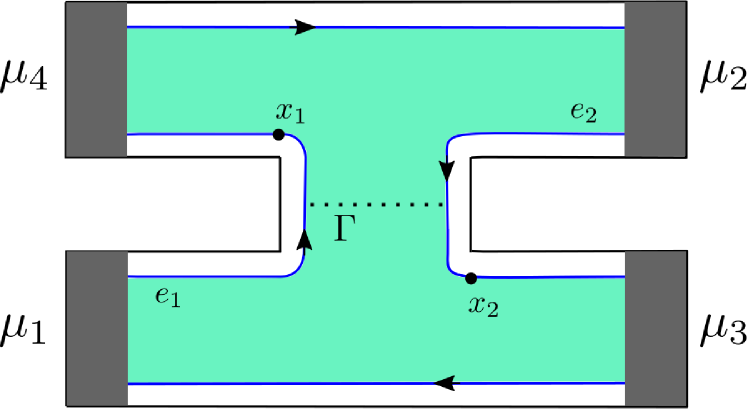
Figure 2: In Figure we give a schematic representation of the device used for the proposed measurement. The green coloured area represents the incompressible electron liquid due to a strong perpendicular magnetic field. The boundary of the electron liquid (blue lines) are the edge channels supporting gapless excitations. As discussed in the main text we only need to focus on edges $e_{1}$ and $e_{2}$, they originate respectively from reservoirs at chemical potential $\mu_{1}$ and $\mu_{2}$. The dotted line represents tunneling between the two edges due to a quantum point contact. Currents are measured at points $x_{1}$ and $x_{2}.$

III Current-Current correlation

In this Section we illustrate the details of our calculations of the correlation of currents measured at the points $x_{1}$ and $x_{2}$ as function of the temperature and of the chemical potentials $\mu_{1}$ and $\mu_{2}$.

The finite frequency current-current correlation reads

$$S(\Omega;x_{1},x_{2})=\frac{1}{2}\int_{-\infty}^{+\infty}d(t_{1}-t_{2})\langle\langle\hat{i}_{1}(t_{1},x_{1})\hat{i}_{2}(t_{2},x_{2})\\ +\hat{i}_{2}(t_{2},x_{2})\hat{i}_{1}(t_{1},x_{1})\rangle\rangle e^{i\Omega(t_{1}-t_{2})}\,.$$ (10)

Similar current-current correlation has been studied in the context of a quantum spin Hall systemLee et al. (2012). Henceforth operators with a ”hat” are to be understood in the Heisenberg representation. We first evaluate the finite frequency correlation $S(\Omega;x_{1},x_{2})$, later, taking the limit for $\Omega\rightarrow 0$, correctly calculate $S(0)$ as it will be clear from the discussion below.

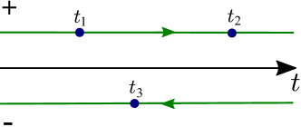
Figure 3: Keldysh contour, the direction of the arrows indicates the ordering of times along the contour. Here $+$ and $-$ indicate the upper and the lower branches, and will be used to define the four components of the Keldysh Green’s function. As example of time ordering on the contour we have $t_{2}$ at later time than $t_{1}$ but at earlier time with respect to $t_{3}$.

Introducing the Keldysh time contour (see Fig. 3), and the Keldysh time ordering operator $T_{K}$ we can rewrite the previous expression as

$$S(\Omega;x_{1},x_{2})=\frac{1}{2}\sum_{\eta=\pm 1}\int_{-\infty}^{+\infty}d(t_{1}-t_{2})e^{i\Omega(t_{1}-t_{2})}\\ \times\langle\langle T_{K}i_{1}(t_{1},x_{1},\eta)i_{2}(t_{2},x_{2},-\eta)\rangle\rangle e^{i\Omega(t_{1}-t_{2})}\,.$$ (11)

Notice that in the above equation we have introduced an index $\eta=\pm 1$ which specify the upper and the lower part of the Keldysh contour.

We assume that the tunneling $H_{T}$ is adiabatically turned on at $t=-\infty$. In order to evaluate Eq.(10) we move to the interaction representation with respect to $H_{0}$, and rewrite Eq.(10) as

$$S(\Omega;x_{1},x_{2})=\frac{1}{2}\sum_{\eta=\pm 1}\int_{-\infty}^{+\infty}d(t_{1}-t_{2})e^{i\Omega(t_{1}-t_{2})}\\ \langle\langle T_{K}i_{1}(t_{1},x_{1},\eta)i_{2}(t_{2},x_{2},-\eta)S_{K}\rangle\rangle\,,$$ (12)

where $S_{K}=T_{K}\exp\{-\frac{i}{\hbar}\int_{K}H_{T}(\tau)d\tau\}$ with $K$ labelling the Keldysh contour. Notice that operators without the ”hat” are to be understood in the interaction representation with respect to $H_{0}$. Expanding $S_{K}$ to the lowest non vanishing order in the tunnelling Hamiltonian we have

$$S(\Omega;x_{1},x_{2})=-\frac{1}{4\hbar^{2}}\sum_{\eta,\eta_{1},\eta_{2}=\pm 1}\eta_{1}\eta_{2}\\ \times\int_{-\infty}^{+\infty}ds_{1}\int_{-\infty}^{+\infty}ds_{2}\int_{-\infty}^{+\infty}d(t_{1}-t_{2})e^{i\Omega(t_{1}-t_{2})}\\ \times\langle\langle T_{K}i_{1}(t_{1},x_{1},\eta)i_{2}(t_{2},x_{2},-\eta)H_{T}(s_{1},\eta_{1})H_{T}(s_{2},\eta_{2})\rangle\rangle\,.$$ (13)

Keeping only connected contributions and dropping terms that are trivially zero by Keldysh integration we may rewrite the previous expression as:

$$S(\Omega;x_{1},x_{2})=-\frac{|\Gamma|^{2}e^{2}\nu v^{2}}{16\pi^{2}\hbar^{2}}\sum_{\eta,\eta_{1},\eta_{2}=\pm 1}\eta_{1}\eta_{2}\times\\ \int_{-\infty}^{+\infty}ds_{1}\int_{-\infty}^{+\infty}ds_{2}\int_{-\infty}^{+\infty}d(t_{1}-t_{2})e^{i\Omega(t_{1}-t_{2})}\Big{\{}\\ \langle T_{K}\partial_{x}\phi_{1}(x_{1},t_{1},\eta)e^{i\sqrt{\nu}\phi_{1}(0,s_{1},\eta_{1})}e^{-i\sqrt{\nu}\phi_{1}(0,s_{2},\eta_{2})}\rangle\\ \times\langle T_{K}\partial_{x}\phi_{2}(x_{2},t_{2},-\eta)e^{-i\sqrt{\nu}\phi_{2}(0,s_{1},\eta_{1})}e^{i\sqrt{\nu}\phi_{2}(0,s_{2},\eta_{2})}\rangle\\ +\,\langle T_{K}\partial_{x}\phi_{1}(x_{1},t_{1},\eta)e^{-i\sqrt{\nu}\phi_{1}(0,s_{1},\eta_{1})}e^{i\sqrt{\nu}\phi_{1}(0,s_{2},\eta_{2})}\rangle\\ \times\langle T_{K}\partial_{x}\phi_{2}(x_{2},t_{2},-\eta)e^{i\sqrt{\nu}\phi_{2}(0,s_{1},\eta_{1})}e^{-i\sqrt{\nu}\phi_{2}(0,s_{2},\eta_{2})}\rangle\Big{\}}\,.$$ (14)

In order to explicitly compute the multiple correlators at finite $\mu_{1}$ and $\mu_{2}$ entering Eq.(14), we recall that, adding a nonzero chemical potential $\mu$ to a chiral Luttinger liquid described by the Hamiltonian of Eq.(4) is equivalent (apart for an over-all constant contribution to the groundstate energy) to the replacement $\partial_{x}\phi(x)\to\partial_{x}\phi(x)-\frac{\mu\sqrt{\nu}}{v}$. Therefore, denoting with $\langle\ldots\rangle_{0}$ the averages computed at $\mu_{1}=\mu_{2}=0$, we obtain

$$\langle T_{K}\partial_{x}\phi_{k}(x,t,\eta)e^{i\sqrt{\nu}\phi_{k}(0,t_{k},\eta_{1})}e^{-i\sqrt{\nu}\phi_{k}(0,t_{2},\eta_{2})}\rangle_{\mu_{k}}=\\ \Big{\{}\langle T_{K}\partial_{x}\phi_{k}(x,t,\eta)e^{i\sqrt{\nu}\phi_{k}(0,t_{1},\eta_{1})}e^{-i\sqrt{\nu}\phi_{k}(0,t_{2},\eta_{2})}\rangle_{0}+\\ -\frac{\mu_{k}\sqrt{\nu}}{v}\langle T_{K}e^{i\sqrt{\nu}\phi_{k}(0,t_{1},\eta_{1})}e^{-i\sqrt{\nu}\phi_{k}(0,t_{2},\eta_{2})}\rangle_{0}\Big{\}}e^{i\nu\mu_{k}(t_{1}-t_{2})}\,,$$ (15)

and similarly for the conjugate expression. Notice that contributions to Eq.(14) proportional to the chemical potentials $\{\mu_{k}\}$ vanish identically after integration over the Keldysh contour. In order to complete the calculation we can use the following identity

$$\langle T_{K}\partial_{x}\phi_{k}(x,t,\eta)e^{i\sqrt{\nu}\phi_{k}(0,t_{1},\eta_{1})}e^{-i\sqrt{\nu}\phi_{k}(0,t_{2},\eta_{2})}\rangle=\\ -i\,\partial_{x}\lim_{\lambda\rightarrow 0}\partial_{\lambda}\langle T_{K}e^{i\lambda\phi_{k}(x,t,\eta)}e^{i\sqrt{\nu}\phi_{k}(0,t_{1},\eta_{1})}e^{-i(\sqrt{\nu}+\lambda)\phi_{k}(0,t_{2},\eta_{2})}\rangle\,.$$ (16)

We finally obtain

$$\langle T_{K}\partial_{x}\phi_{k}(x,t,\eta)e^{i\sqrt{\nu}\phi_{k}(0,t_{1},\eta_{1})}e^{-i\sqrt{\nu}\phi_{k}(0,t_{2},\eta_{2})}\rangle_{0}=$$

$$\frac{\sqrt{\nu}\pi}{\hbar\beta v}\Big{(}\cot\left\{\frac{\pi}{\hbar\beta}\left[i(t-t_{1}-x/v)+\tau_{c}\,\sigma_{\eta,\eta_{1}}(t-t_{1})\right]\right\}$$

$$-\cot\left\{\frac{\pi}{\hbar\beta}\left[i(t-t_{2}-x/v)+\tau_{c}\,\sigma_{\eta,\eta_{2}}(t-t_{2})\right]\right\}\Big{)}$$

$$\times G^{(\nu)}_{\eta_{1},\eta_{2}}(t_{1}-t_{2})\>\>\>\>.$$ (17)

In Eq.(17), we have set $\beta=(k_{B}T)^{-1}$. Also, we have defined $\sigma_{\eta,\eta^{\prime}}(t-t^{\prime})=[(\eta+\eta^{\prime}){\rm sgn}(t-t^{\prime})+\eta^{\prime}-\eta]/2$ and have introduced the cutoff time $\tau_{c}=l_{c}/v$, with $l_{c}$ being a short-distance cutoff length. Moreover, we have introduced the Keldysh Green function $G^{(\nu)}_{\eta_{1},\eta_{2}}(t_{1}-t_{2})=\langle T_{K}e^{i\sqrt{\nu}\phi_{k}(0,t_{1},\eta_{1})}e^{-i\sqrt{\nu}\phi_{k}(0,t_{2},\eta_{2})}\rangle_{0}$, given by

$$G^{(\nu)}_{\eta_{1},\eta_{2}}(t_{1}-t_{2})=l_{c}^{\nu}$$

$$\times\left(\frac{\hbar\beta v}{\pi}\sin\left\{\frac{\pi}{\hbar\beta}[i(t_{1}-t_{2})\sigma_{\eta_{1},\eta_{2}}(t_{1}-t_{2})+\tau_{c}]\right\}\right)^{-\nu}$$ (18)

The cutoff-dependent contribution to the argument of the cotangent functions at the second and at the third line of Eq.(17) is effective only when $t-t_{1}-x/v\sim 0$ (second line), or when $t-t_{1}-x/v\sim 0$ (third line). This enables us to set $\sigma_{\eta,\eta_{1}}(t-t_{1})=\sigma_{\eta,\eta_{1}}(x/v)=\eta_{1}$ (second line), and $\sigma_{\eta,\eta_{2}}(t-t_{2})=\sigma_{\eta,\eta_{2}}(x/v)=\eta_{2}$ (third line). As a result, we may eventually rewrite Eq.(17) as

$$\langle T_{K}\partial_{x}\phi_{k}(x,t,\eta)e^{i\sqrt{\nu}\phi_{k}(0,t_{1},\eta_{1})}e^{-i\sqrt{\nu}\phi_{k}(0,t_{2},\eta_{2})}\rangle_{0}=$$

$$\frac{\sqrt{\nu}}{v}\left[\xi_{\eta_{1}}\left(t-t_{1}-\frac{x}{v}\right)-\xi_{\eta_{2}}\left(t-t_{2}-\frac{x}{v}\right)\right]$$

$$\times G^{(\nu)}_{\eta_{1},\eta_{2}}(t_{1}-t_{2})\>\>\>\>,$$ (19)

with

$$\xi_{\eta}(t)=\frac{\pi}{\hbar\beta}\cot\left[\frac{\pi}{\hbar\beta}(it+\eta\tau_{c})\right]\,\>\>\>.$$ (20)

Taking into account the result in Eq.(19), it is now

possible to explicitly compute $S(\Omega;x_{1},x_{2})$. Introducing the Fourier transform of $G_{\eta_{1},\eta_{2}}^{(\nu)}$ and of $\xi_{\eta}$ (see Appendix A for details) we obtain

$$S(\Omega;x_{1},x_{2})=\frac{|\Gamma|^{2}e^{2}\nu^{2}}{4\pi^{2}\hbar^{2}}\>e^{i\Omega(x_{1}-x_{2})}\sum_{\eta_{1},\eta_{2}}\eta_{1}\eta_{2}\\ \times\biggl{\{}[\xi_{\eta_{1}}(\Omega)\xi_{\eta_{1}}(-\Omega)+\xi_{\eta_{2}}(\Omega)\xi_{\eta_{2}}(-\Omega)]G_{\eta_{1},\eta_{2}}^{(2\nu)}(\nu\Delta\mu)\\ -\xi_{\eta_{1}}(\Omega)\xi_{\eta_{2}}(-\Omega)G_{\eta_{1},\eta_{2}}^{(2\nu)}(\nu\Delta\mu+\Omega)\\ -\xi_{\eta_{1}}(-\Omega)\xi_{\eta_{2}}(\Omega)G_{\eta_{1},\eta_{2}}^{(2\nu)}(\nu\Delta\mu-\Omega)\biggr{\}}\,,$$ (21)

with $\Delta\mu=\mu_{1}-\mu_{2}$. Using the explicit formulas for $G_{\eta_{1}\eta_{2}}^{(\nu)}$ and $\xi_{\eta}(\Omega)$ (see Eqs.(38,39,40,41,43) ) we perform the sum over the Keldysh indices. Taking the limit for $\Omega\rightarrow 0$ eventually we obtain

$$S(0)=2i\left(\frac{\hbar\beta}{2\pi}\right)^{1-2\nu}\frac{e^{2}\nu^{2}\tau_{c}^{2\nu}|\Gamma|^{2}}{\hbar^{2}\pi\Gamma(2\nu)}\>\sinh\left(\frac{\beta\nu\Delta\mu}{2}\right)\\ \times\left|\Gamma\left(\nu+\frac{i\beta\nu\Delta\mu}{2\pi}\right)\right|^{2}\\ \times\left[\psi(\nu+\frac{i\beta\nu\Delta\mu}{2\pi})-\psi(\nu-\frac{i\beta\nu\Delta\mu}{2\pi})\right]\,.$$ (22)

To recover a compact notation, in Eq.(22) we have expressed $S(0)$ in terms of Euler Gamma function $\Gamma(z)$ and of its logarithmic derivative, the digamma function $\psi(z)=\partial_{z}[\ln\Gamma(z)]$. As anticipated, in order to obtain the correct result for $S(0)$, one has to first perform the calculation of $S(\Omega;x_{1},x_{2})$ at finite $\Omega$ and then take the limit $\Omega\to 0$ at the end of the calculation, thus avoiding problems related to $\xi_{\eta}(\Omega)$ being ill-defined as $\Omega\to 0$ (see appendix A for details). Taking $\nu=1$ in Eq.(22) reproduces the known result for non-interacting electronsBüttiker (1992) which we discuss in detail in Appendix B.

In the next Section we will look at the ratio $S(0)/i_{T}$, with $i_{T}$ being the tunneling current across the QPC. For the reader’s convenience we report below the standard resultWen (1991)

$$i_{T}=\frac{2q}{\hbar^{2}\Gamma(2\nu)}|\Gamma|^{2}\tau_{c}^{2\nu}\left(\frac{\hbar\beta}{2\pi}\right)^{1-2\nu}\\ \times\sinh\left(\frac{\beta\nu\Delta\mu}{2}\right)\left|\Gamma\left(\nu+i\frac{\beta\Delta\mu\nu}{2\pi}\right)\right|^{2}\,.$$ (23)

The generalization of Eq.(23), beyond perturbative expansion, was calculated exactly by Bethe-ansatz in Refs.[Fendley et al., 1995a, b; Fendley and Saleur, 1996].

IV Fractional statistics detection from current-current correlation

Equation (22) is the main result of this Article, in this Section we discuss its consequences.

As a first comment we notice that in analogy with the result in Eq.(3), we find that $S(0)=0$ for $\mu_{1}=\mu_{2}$. This is consistent with Büttiker’s result of Ref.[Büttiker, 1992] for the non-interacting case ($\nu=1$), and it is now generalized to the case of Laughlin fractions. Such a result for $\nu=1$ is easily shown to be in agreement with the fluctuation-dissipation theorem. Indeed for non-interacting electrons the equilibrium correlation function between currents measured at drains $\alpha$ and $\beta$, $i_{\alpha}$ and $i_{\beta}$, satisfies the relation

$$\int_{-\infty}^{+\infty}\>\langle\langle\{i_{\alpha}(t),i_{\beta}(0)\}\rangle\rangle dt=2({\bf G}_{\alpha,\beta}+{\bf G}_{\beta,\alpha})k_{B}T\;\;,$$ (24)

with $\bf{G}_{\alpha,\beta}$ being the dc conductance between terminals $\alpha$ and $\beta$. In fact, in the particular geometry we are considering here, no electric current can flow between $x_{1}$ and $x_{2}$, because of the chiral propagation along the edge channels. Therefore, we have shown that a result similar to that of Ref.[Büttiker, 1992] also applies to currents at the edges of a FQH liquid. Moreover, Eq.(3) shows that, for any Laughlin filling $\nu$, the current-current correlation is negative, suggesting that the beam splitter geometry we consider highlights the exclusion statistics character of Laughlin’s quasi-particlesHaldane (1991). This result agrees with Ref.[Safi et al., 2001] for their case $\nu=1/3$ but not for $\nu\leq 1/5$, and it is in contrast with Refs.[Kim et al., 2005; Campagnano et al., 2012, 2013]. We suspect that this is somehow related to the different geometries involved, and we will investigate this issue in future works.

We also notice that negative correlations are found in Ref.[Rosenow et al., 2015] where current-current correlation is studied for a beam of diluted anyons impinging on a beam splitter, analysis complementary to the study reported here.

Besides the results outlined above, our most important finding is that, combining together Eq.(22) and Eq.(23), it is possible to propose a way to directly measure the fractional statistics of LQPs. A key observation is now that, by setting $\Delta\mu=eV$, where $V$ is the voltage bias between $e_{1}$ and $e_{2}$, the argument of the Gamma and the digamma functions in Eqs.(22,23) can be rewritten as $\zeta=\nu+i\frac{\beta qV}{2\pi}$. Roughly speaking, one might say that $\Re e(\zeta)$ carries information about the fractional statistics, while $\Im m(\zeta)$ carries information about the fractional charge. Therefore, one might expect that either information can be extracted, according to whether one considers the formulas in the limit $|\Re e(\zeta)/\Im m(\zeta)|\gg 1$, or $|\Re e(\zeta)/\Im m(\zeta)|\ll 1$.

Let us discuss first the case $|\Re e(\zeta)/\Im m(\zeta)|\ll 1$, corresponding to $|eV|\gg k_{B}T$. In this regime, an appropriate approximation for Eqs.(22,23) can be derived by using Stirling’s formula for the $\Gamma$-functions, that is

$$\Gamma(z)\approx\sqrt{2\pi}\>(z-1)^{z-\frac{1}{2}}\>e^{-z+1}\>\>\>\>,$$ (25)

valid for $|z|\gg 1$. Using Eq.(25), one finds the following asymptotic expansions for $S(0)$ and $i_{T}$ (assuming $V>0$)

$$S(0) \approx -\frac{2\pi q^{2}|\Gamma|^{2}\tau_{c}^{2\nu}}{\hbar^{2\nu+1}~{}\Gamma[2\nu]}(qV)^{2\nu-1}$$

$$i_{T} \approx \frac{2\pi q|\Gamma|^{2}\tau_{c}^{2\nu}}{\hbar^{2\nu+1}\Gamma[2\nu]}(qV)^{2\nu-1}\>\>\>\>.$$ (26)

Eqs.(26) suggest that, for $|eV|\gg k_{B}T$, the fractional charge $q$ can be directly probed by looking at the ratio $q=|S(0)|/i_{T}$ between two directly measurable quantities such as $S(0)$ and $i_{T}$, which is the main idea typically implemented in shot-noise based measurements of the fractional charge (notice that here, instead, we look at correlation between currents at different drains).

In the complementary limit, in order to directly access to informations on the fractional statistics, one has rather to consider the thermal regime, namely, $|eV|\ll k_{B}T$. In this regime, the limiting formulas for Eqs.(22,23) can be recovered by expanding the Gamma and the digamma functions to leading order in $\Im m(\zeta)/\Re e(\zeta)$, obtaining

$$S(0) \approx -\frac{q^{2}|\Gamma|^{2}\tau_{c}^{2\nu}}{\hbar^{2\nu+1}~{}\Gamma[2\nu]}\left(\frac{\beta}{2\pi}\right)^{1-2\nu}(\beta qV)^{2}\{\Gamma^{{}^{\prime\prime}}[\nu]\Gamma[\nu]-(\Gamma^{{}^{\prime}}[\nu])^{2}\}\,,$$

$$i_{T} \approx \frac{q|\Gamma|^{2}\tau_{c}^{2\nu}\Gamma^{2}[\nu]}{\hbar^{2\nu+1}~{}\Gamma[2\nu]}\left(\frac{\beta}{2\pi}\right)^{1-2\nu}(\beta qV)\,.$$ (27)

From Eqs.(27) one therefore obtains

$$\frac{|S(0)|}{i_{T}}=\left[\frac{q^{2}\pi^{2}V}{6k_{B}T}\right]\gamma(\nu)\>\>\>\>,$$ (28)

with $\gamma(\nu)=(6/\pi^{2})\partial_{z}^{2}\ln\Gamma(z)\big{|}_{z=\nu}$. Except for the factor $\gamma(\nu)$, the result in Eq.(28) is the same one would obtain for non-interacting electrons ($\nu=1$) by simply replacing $e$ with $q$. Therefore, the additional factor $\gamma(\nu)$ is not a feature simply related to the fractional charge of LQPs—it is a clear signature of the quasi-particle fractional statistics which, as we propose, can be directly measured by looking at currents correlations probed in the appropriate thermal regime. We report here, for the readers’ convenience, some numerical values of $\gamma(\nu)$, $\gamma(1)=$1, $\gamma(1/3)\simeq 6.18$, $\gamma(1/5)\simeq 15.97$.

As a final remark, we notice that the reason to look at the correlation of currents measured at different drains lies in the fact that, if one considers noise of the tunneling current, i.e. $S_{i_{T}}=(1/2)\int dt\langle\langle\{i_{T}(0),i_{T}(t)\}\rangle\rangle$, one would obtainKane and Fisher (1994)

$$S_{i_{T}}=\frac{2q^{2}}{\hbar^{2}\Gamma(2\nu)}|\Gamma|^{2}\tau_{c}^{2\nu}\left(\frac{\hbar\beta}{2\pi}\right)^{1-2\nu}\\ \times\cosh\left(\frac{\beta\nu\Delta\mu}{2}\right)\left|\Gamma\left(\nu+i\frac{\beta\Delta\mu\nu}{2\pi}\right)\right|^{2}\,.$$ (29)

Such a quantity normalized to the tunneling current $i_{T}$ of Eq.(23), i.e. the Fano factor, only carries information about the quasi-particles’ charge but not their statistics.

V Summary and Outlook

We have discussed the correlation of currents measured at separate drains in a beam splitter-like geometry for fractional quantum Hall systems at Laughlin filling factors. Because of the chiral propagation of LQPs along the edge channels we have proved (within perturbation theory) that the equilibrium correlation, i.e. for $\mu_{1}=\mu_{2}$, is zero, as it was found for chiral fermions ($\nu=1$). Using Keldysh technique we have also obtained expressions for the stationary out of equilibrium case and show how a correlation measurements carries information about the fractional statistics. Our findings suggest an anti-bunching character of the LQPs.

In perspective our result might also provide a useful tool to investigate more exotic filling fractions like for instance $\nu=2/3$ where neutral counter-propagating modes have been predictedKane et al. (1994); Kane and Fisher (1995) and recently observedBid et al. (2010); Gross et al. (2012); Gurman et al. (2012), but still in the need of a thorough characterisation.

In such systems even for both the measuring points $x_{1}$ and $x_{2}$ situated after the QPC, due to the counter-propagating modes and their interaction with the charge modes, one might expect a signal propagation between these two points—giving rise to a non zero equilibrium correlation. We will to investigate this possibility as tool to study counter-propagating modes in future works. In addition, we also plan to expand our work to analyze the relation between correlations and fractional statistics-related interaction among particles with fractionalized quantum numbersBernevig et al. (2001a, b); Bernevig et al. (2003).

Appendix A Green’s functions

In this Appendix, we provide the details of the calculation of the Green’s functions we use to compute the current-current correlation, and their corresponding Fourier transforms. The first quantities we need are the correlation functions of vertex operators evaluated on branches $\eta_{1},\eta_{2}$ of the Keldysh path,

$$G_{\eta_{1},\eta_{2}}^{(\nu)}(t_{1},t_{2})=\langle T_{K}e^{i\sqrt{\nu}\phi_{k}(t_{1},\eta_{1})}e^{-i\sqrt{\nu}\phi_{k}(t_{2},\eta_{2})}\rangle_{0}\;\;\;\;.$$ (30)

A standard bosonization calculation yields the result in Eq.(18),

$$G_{\eta_{1},\eta_{2}}^{(\nu)}(t_{1},t_{2})=l_{c}^{\nu}\left(\frac{\hbar\beta v}{\pi}\right)^{-\nu}\sin^{-\nu}\left[\frac{\pi}{\hbar\beta}(it\,\sigma_{\eta_{1},\eta_{2}}(t_{1}-t_{2})+\tau_{c})\right]\>\>\>\>.$$ (31)

For the sake of clarity, we list the Keldysh Green functions corresponding to the four possible choice of the Keldysh indices:

$$G_{+,+}^{(\nu)}(t) = l_{c}^{\nu}\left(\frac{\hbar\beta v}{\pi}\right)^{-\nu}\>\sin^{-\nu}\left[\frac{\pi}{\hbar\beta}(i|t|+\tau_{c})\right],$$

$$G_{-,-}^{(\nu)}(t) = l_{c}^{\nu}\left(\frac{\hbar\beta v}{\pi}\right)^{-\nu}\>\sin^{-\nu}\left[\frac{\pi}{\hbar\beta}(-i|t|+\tau_{c})\right],$$

$$G_{-,+}^{(\nu)}(t) = l_{c}^{\nu}\left(\frac{\hbar\beta v}{\pi}\right)^{-\nu}\>\sin^{-\nu}\left[\frac{\pi}{\hbar\beta}(it+\tau_{c})\right],$$

$$G_{+,-}^{(\nu)}(t) = l_{c}^{\nu}\left(\frac{\hbar\beta v}{\pi}\right)^{-\nu}\>\sin^{-\nu}\left[\frac{\pi}{\hbar\beta}(-it+\tau_{c})\right]\,.$$ (32)

Next we compute the Fourier transform of Eqs.(32) defined as,

$$G_{\eta_{1},\eta_{2}}^{(\nu)}(\omega)=\int_{-\infty}^{+\infty}dt\,e^{i\omega t}\,G_{\eta_{1},\eta_{2}}^{(\nu)}(t)\>\>\>\>.$$

In computing $G_{\eta_{1},\eta_{2}}^{(\nu)}(\omega)$, it is useful to start with $G_{-,+}^{(\nu)}(\omega)$ and with $G_{+,-}^{(\nu)}(\omega)$. Moreover, in view of the identity $G_{-,+}^{(\nu)}(\omega)=G_{+,-}^{(\nu)}(-\omega)$ (which is readily proved from the definition of the Keldysh Green functions), one concludes that it is enough to just compute $G_{-,+}^{(\nu)}(\omega)$. In order to do so, we notice that the branch points of $G_{-,+}^{(\nu)}(t)$ are located at $t_{n}=i(\tau_{c}+\hbar\beta n)$, with $n=0,\pm 1,\ldots$. Therefore, to make sure that no branch cuts intersect the real axis in computing $G_{-,+}^{(\nu)}(\omega)$, we chose the phase branch so that $-\pi\leq{\rm arg}(it)<\pi$ and, accordingly, the branch cuts are all horizontal. Having stated this, $G_{-,+}^{(\nu)}(\omega)$ takes the following integral representation

$$G_{-,+}^{(\nu)}(\omega)=\\ l_{c}^{\nu}\left(\frac{\hbar\beta v}{2\pi}\right)^{-\nu}\int_{-\infty}^{\infty}\>dt\>e^{i\omega t}[(-i)e^{-\frac{\pi t}{\hbar\beta}}e^{i\delta}-(-i)e^{\frac{\pi t}{\hbar\beta}}e^{-i\delta}]^{-\nu}\\ =\frac{2l_{c}^{\nu}}{v^{\nu}}\left(\frac{\hbar\beta}{2\pi}\right)^{1-\nu}\int_{0}^{\infty}\>du\>e^{i\frac{\hbar\omega\beta}{\pi}u}[(-i)e^{-u}e^{i\delta}-(-i)e^{u}e^{-i\delta}]^{-\nu}\\ +\frac{2l_{c}^{\nu}}{v^{\nu}}\left(\frac{\hbar\beta}{2\pi}\right)^{1-\nu}\int^{0}_{-\infty}\>du\>e^{i\frac{\hbar\omega\beta}{\pi}u}[(-i)e^{-u}e^{i\delta}-(-i)e^{u}e^{-i\delta}]^{-\nu}\\ =\frac{2l_{c}^{\nu}}{v^{\nu}}\left(\frac{\hbar\beta}{2\pi}\right)^{1-\nu}e^{i\pi\nu/2}\int_{0}^{\infty}\>du\>e^{\left(i\frac{\hbar\omega\beta}{\pi}-\nu\right)u}[1-e^{-2u}]^{-\nu}\\ +\frac{2l_{c}^{\nu}}{v^{\nu}}\left(\frac{\hbar\beta}{2\pi}\right)^{1-\nu}e^{-i\pi\nu/2}\int^{0}_{-\infty}\>du\>e^{\left(i\frac{\hbar\omega\beta}{\pi}+\nu\right)u}[1-e^{2u}]^{-\nu}\,.$$ (33)

In Eq.(33) we have set $\delta=\pi\tau_{c}/\hbar\beta$ and have taken advantage of the fact that, in the last two lines, it was possible to drop the terms depending on the regularizator $\delta$. Going through straightforward manipulation we can readily trade Eq.(33) for a known integral representation of the Beta-function, that is

$$B(x,y)=\frac{\Gamma(x)\Gamma(y)}{\Gamma(x+y)}=\int_{0}^{1}\>dw\>w^{x-1}(1-w)^{y-1}\,.$$ (34)

To do so, we resort to the integration variable $w=e^{-2u}$ ($w=e^{2u}$ ) in the first (second) integral of Eq.(33), so that we eventually obtain

$$G_{-,+}^{(\nu)}(\omega)=\\ \left(\frac{l_{c}}{v}\right)^{\nu}\left(\frac{\hbar\beta}{2\pi}\right)^{1-\nu}e^{-i\pi\nu/2}\>\int_{0}^{1}\>dw\>w^{i\frac{\hbar\omega\beta}{2\pi}+\frac{\nu}{2}-1}(1-w)^{-\nu}\\ +\left(\frac{l_{c}}{v}\right)^{\nu}\left(\frac{\hbar\beta}{2\pi}\right)^{1-\nu}e^{i\pi\nu/2}\>\int_{0}^{1}\>dw\>w^{-i\frac{\hbar\omega\beta}{2\pi}+\frac{\nu}{2}-1}(1-w)^{-\nu}\,.$$ (35)

Comparing Eq.(35) to Eq.(34), we eventually find

$$G_{-,+}^{(\nu)}(\omega)=\\ \left(\frac{l_{c}}{v}\right)^{\nu}\left(\frac{\hbar\beta}{2\pi}\right)^{1-\nu}\Gamma(1-\nu)\left[e^{i\pi\nu/2}\frac{\Gamma\left(\frac{\nu}{2}-i\frac{\hbar\omega\beta}{2\pi}\right)}{\Gamma\left(1-\frac{\nu}{2}-i\frac{\hbar\omega\beta}{2\pi}\right)}\right.+\\ \left.e^{-i\pi\nu/2}\frac{\Gamma\left(\frac{\nu}{2}+i\frac{\hbar\omega\beta}{2\pi}\right)}{\Gamma\left(1-\frac{\nu}{2}+i\frac{\hbar\omega\beta}{2\pi}\right)}\right]\,.$$ (36)

Finally, using the identity

$$\Gamma(z)\Gamma(1-z)=\frac{\pi}{\sin(\pi z)}\>\>\>\>,$$ (37)

we can recast Eq.(36) into the form

$$G_{-,+}^{(\nu)}(\omega)=\frac{l_{c}^{\nu}}{v^{\nu}\Gamma(\nu)}\left(\frac{\hbar\beta}{2\pi}\right)^{1-\nu}e^{\frac{\hbar\omega\beta}{2}}\left|\Gamma\left(\frac{\nu}{2}+i\frac{\hbar\omega\beta}{2\pi}\right)\right|^{2}\,.$$ (38)

Eq.(38) also implies

$$G_{+,-}^{(\nu)}(\omega)=\frac{l_{c}^{\nu}}{v^{\nu}\Gamma(\nu)}\left(\frac{\hbar\beta}{2\pi}\right)^{1-\nu}e^{-\frac{\hbar\omega\beta}{2}}\left|\Gamma\left(\frac{\nu}{2}+i\frac{\hbar\omega\beta}{2\pi}\right)\right|^{2}\,.$$ (39)

Following exactly the same strategy of splitting the integral over $t$ into an integral from $-\infty$ to 0 plus and integral from $0$ to $\infty$ and separately manipulating the two integrals as we have done before, one eventually finds

$$G_{+,+}^{(\nu)}(\omega)=\frac{l_{c}^{\nu}e^{-i\pi\nu/2}}{v^{\nu}\Gamma(\nu)\cos\left(\frac{\pi\nu}{2}\right)}\left(\frac{\hbar\beta}{2\pi}\right)^{1-\nu}\\ \times\cosh\left(\frac{\hbar\omega\beta}{2}\right)\left|\Gamma\left(\frac{\nu}{2}+i\frac{\hbar\omega\beta}{2\pi}\right)\right|^{2}\,,$$ (40)

and

$$G_{-,-}^{(\nu)}(\omega)=\frac{l_{c}^{\nu}e^{i\pi\nu/2}}{v^{\nu}\Gamma(\nu)\cos\left(\frac{\pi\nu}{2}\right)}\left(\frac{\hbar\beta}{2\pi}\right)^{1-\nu}\\ \times\cosh\left(\frac{\hbar\omega\beta}{2}\right)\left|\Gamma\left(\frac{\nu}{2}+i\frac{\hbar\omega\beta}{2\pi}\right)\right|^{2}\,.$$ (41)

Eqs.(38,39,40,41) provide us with the Fourier transforms of the Keldysh Green functions which we used in the main text to compute the current correlations. Additional function one needs in performing the calculation are the Fourier transform of $\xi_{\pm}(t)$. These are given by

$$\xi_{\eta}(\omega)=\int_{-\infty}^{\infty}\>dt\>e^{i\omega t}\xi_{\eta}(t)\\ =i\int_{-\infty}^{\infty}\>du\>e^{i\frac{\hbar\omega\beta}{\pi}u}\left\{\frac{e^{u}e^{-i\eta\frac{\pi\tau_{c}}{\hbar\beta}}+e^{-u}e^{i\eta\frac{\pi\tau_{c}}{\hbar\beta}}}{e^{u}e^{-i\eta\frac{\pi\tau_{c}}{\hbar\beta}}-e^{-u}e^{i\eta\frac{\pi\tau_{c}}{\hbar\beta}}}\right\}\,,$$ (42)

where we have set $u\equiv t\pi/\hbar\beta$. When $\omega\neq 0$, a straightforward application of residue theorem gives

$$\xi_{+}(\omega) = \int_{-\infty}^{\infty}\>d\omega\>e^{i\omega t}\xi_{+}(t)=\frac{2\pi e^{-\omega\tau_{c}}}{1-e^{-\hbar\beta\omega}}\,,$$

$$\xi_{-}(\omega) = \int_{-\infty}^{\infty}\>d\omega\>e^{i\omega t}\xi_{-}(t)=\frac{2\pi e^{\omega\tau_{c}}}{e^{\hbar\beta\omega}-1}\,.$$ (43)

The integrals in Eq.(42) are ill-defined if $\omega=0$, this motivates the need of first computing the current current correlation in Fourier space at finite frequency $\Omega$, and then only afterwards taking $\Omega\to 0$.

Appendix B Current-current correlation for chiral fermions.

In this Appendix to check the consistency of the formulas we derived in section III with the standard results obtained by Büttiker in the non-interacting case, we derive the current-current correlation in the case Integer Quantum Hall (IQH)-effect at filling $\nu=1$. At $\nu=1$, IQH-edges $e_{1}$ and $e_{2}$ (see Fig. 2) are described by the non-interacting chiral fermion Hamiltonian:

$$H_{0}=-i\hbar v\sum_{j=1}^{2}\int dx:\psi_{j}^{\dagger}(x)\partial_{x}\psi_{j}(x):\;\;\;\;,$$ (44)

with $v$ being the Fermi velocity. In the momentum basis, the chiral fermionic fields $\psi_{i}(x)$ take the mode-expansion

$$\psi_{j}(x)=\frac{1}{\sqrt{\mathcal{L}_{j}}}\sum_{k_{j}}e^{ik_{j}x}c_{k_{j},j}\,.$$ (45)

In Eq.(45), we use $\mathcal{L}_{i}$ to denote the length of the edge $i$, which we assume to be large enough to be irrelevant for our final result. The double columns $:\>:$ denote normal ordering with respect to the groundstate $|GS\rangle=\prod_{i=1,2;\epsilon(k_{j})\leq 0}c_{k_{j},i}^{\dagger}|0\rangle$. $c_{k_{j},i}$ is the electron annihilation operator for a state with momentum $k_{j}$ on edge $i$. Creation and annihilation operators in the momentum basis satisfy the standard fermionic anti-commutations rules, $\{c_{k_{j},j}^{\dagger},c_{k_{j^{\prime}}^{\prime},j^{\prime}}\}=\delta_{k_{j},k_{j^{\prime}}^{\prime}}\delta_{j,j^{\prime}}$, $\{c_{k_{j},j},c_{k_{j^{\prime}}^{\prime},j^{\prime}}\}=0$. To account for the chemical potential bias between the edges, we assume that, in absence of tunnelling, each edge $i$ is at equilibrium with a reservoir at chemical potential $\mu_{i}$.

In order to allow for electrons to tunnel between the two edges, we consider the tunneling Hamiltonian $H_{T}$ given by

$$H_{T}=\Gamma_{e}\psi^{\dagger}_{1}(0)\psi_{2}(0)+{\rm h.c.}\>\>\>\>.$$ (46)

The current density operator at site $x$ of edge $i$ is given by $i_{i}(x)=ev:\psi^{\dagger}(x)\psi(x):$. The current correlation function between point $x_{1}$ on $e_{1}$ and point $x_{2}$ on $e_{2}$ (cfr Fig. 2) is defined as in Eq.(10) and, resorting again to the Keldysh formalism we use in section III, we readily find that the corresponding zero-frequency limit, $S(0)$, is given by

$$S(0)=\frac{e^{2}v^{2}}{2}\sum_{\eta=\pm 1}\int_{-\infty}^{+\infty}d(t_{1}-t_{2})\\ \langle\langle T_{K}:\hat{\psi}_{1}^{\dagger}(x_{1},t_{1}+\eta\,0^{+},\eta)\hat{\psi}_{1}(x_{1},t_{1},\eta):\\ :\hat{\psi}_{2}^{\dagger}(x_{2},t_{2}-\eta\,0^{+},-\eta)\hat{\psi}_{2}(x_{2},t_{2},-\eta):\rangle\rangle\>.$$ (47)

(note that, in order to preserve the correct ordering of the fermionic operators under the action of $T_{K}$, in Eq.(47) we introduced the infinitesimal positive quantity $0^{+}$ as a regularizator). Assuming a weak tunneling rate between the edges to recover consistency with the analysis of section III, we compute $S(0)$ to second order in $H_{T}$, obtaining

$$S(0)=-\frac{|\Gamma_{e}|^{2}e^{2}v^{2}}{4\hbar^{2}}\sum_{\eta,\eta_{1},\eta_{2}=\pm 1}\eta_{1}\eta_{2}\int_{-\infty}^{+\infty}d(t_{1}-t_{2})\int_{-\infty}^{+\infty}ds_{1}\int_{-\infty}^{+\infty}ds_{2}\\ \times\left[\mathcal{G}^{(1)}_{\eta_{2},\eta}(-x_{1},s_{2}-t_{1})\mathcal{G}^{(1)}_{\eta,\eta_{1}}(x_{1},t_{1}-s_{1})\mathcal{G}^{(2)}_{\eta_{1},-\eta}(-x_{2},s_{1}-t_{2})\mathcal{G}^{(2)}_{-\eta,\eta_{2}}(x_{2},t_{2}-s_{2})\right.\\ +\left.\mathcal{G}^{(1)}_{\eta_{1},\eta}(-x_{1},s_{1}-t_{1})\mathcal{G}^{(1)}_{\eta,\eta_{2}}(x_{1},t_{1}-s_{2})\mathcal{G}^{(2)}_{\eta_{2},-\eta}(-x_{2},s_{2}-t_{2})\mathcal{G}^{(2)}_{-\eta,\eta_{1}}(x_{2},t_{2}-s_{1})\right],$$ (48)

with the fermionic Keldysh Green function $\mathcal{G}^{(i)}_{\eta_{1},\eta_{2}}(x_{1}-x_{2},t_{1}-t_{2})=-i\langle T_{K}\psi_{i}(x_{1},t_{1},\eta_{1})\psi^{\dagger}_{i}(x_{2},t_{2},\eta_{2})\rangle$, with $\psi_{i}(x,t)$ being the fermion fields in the interaction representation with respect the Hamiltonian $H_{0}$. Moving to Fourier space, we may rewrite Eq.(48) as

$$S(0)=\frac{|\Gamma_{e}|^{2}e^{2}v^{2}}{2\hbar^{2}}\sum_{\eta,\eta_{1},\eta_{2}=\pm 1}\eta_{1}\eta_{2}\int_{-\infty}^{+\infty}\frac{d\omega}{2\pi}\\ \times\left[\mathcal{G}^{(1)}_{\eta_{2},\eta}(-x_{1},\omega)\mathcal{G}^{(1)}_{\eta,\eta_{1}}(x_{1},\omega)\mathcal{G}^{(2)}_{\eta_{1},-\eta}(-x_{2},\omega)\mathcal{G}^{(2)}_{-\eta,\eta_{2}}(x_{2},\omega)\right],$$ (49)

with the singe-fermion Keldysh Green functions in Fourier space given byCampagnano et al. (2013)

$$\mathcal{G}^{(i)}_{++}(x,\omega)= \frac{i}{v}e^{i\omega x/v}[f(\hbar\omega-\mu_{i})-\Theta(x)]\,,$$ (50)

$$\mathcal{G}^{(i)}_{+-}(x,\omega)= \frac{i}{v}e^{i\omega x/v}f(\hbar\omega-\mu_{i})\,,$$ (51)

$$\mathcal{G}^{(i)}_{-+}(x,\omega)= -\frac{i}{v}e^{i\omega x/v}[1-f(\hbar\omega-\mu_{i})]\,,$$ (52)

$$\mathcal{G}^{(i)}_{--}(x,\omega)= \frac{i}{v}e^{i\omega x/v}[f(\hbar\omega-\mu_{i})-\Theta(-x)]\,.$$ (53)

In Eqs.(53) $f(\omega)$ denotes the Fermi-Dirac distribution function $f(\omega)=[1+\exp(\beta\hbar\omega)]^{-1}$, while $\Theta(x)$ is the Heaviside step function regularized so that $\Theta(0)=1/2$.

Performing the sum over the Keldysh indices, using Eqs.(53) for both $x_{1}$ and $x_{2}>0$ , we obtain

$$S(0)=-\frac{e^{2}|\Gamma_{e}|^{2}}{2\pi v^{2}\hbar^{2}}\int_{-\infty}^{+\infty}d\omega\left[f(\hbar\omega-\mu_{1})-f(\hbar\omega-\mu_{2})\right]^{2}.$$ (54)

Notice that in Eq.(9) the tunneling amplitude $\Gamma$ has the dimension of an energy, while $\Gamma_{e}$ has the dimensions of an energy times a length. Eq.(22) evaluated for $\nu=1$ reproduce Eq.(54) by taking $\Gamma=\Gamma_{e}/(2\pi l_{c})$, which is indeed consistent with the bosonization identityvon Delft and Schoeller (1998) $\psi_{i}(x)=e^{-i\phi_{i}(x)}/\sqrt{2\pi l_{c}}$ .

References

- Büttiker (1992) M. Büttiker, Phys. Rev. B 46, 12485 (1992).
- Tsui et al. (1982) D. C. Tsui, H. L. Stormer, and A. C. Gossard, Phys. Rev. Lett. 48, 1559 (1982).
- Laughlin (1983) R. B. Laughlin, Phys. Rev. Lett. 50, 1395 (1983).
- Arovas et al. (1984) D. Arovas, J. R. Schrieffer, and F. Wilczek, Phys. Rev. Lett. 53, 722 (1984).
- Nayak et al. (2008) C. Nayak, S. H. Simon, A. Stern, M. Freedman, and S. Das Sarma, Rev. Mod. Phys. 80, 1083 (2008).
- Wen (2004) X. G. Wen, Quantum Field Theory Of Many-Body Systems: From The Origin Of Sound To An Origin Of Light And Electrons (Oxford University Press, 2004).
- de Picciotto et al. (1997) R. de Picciotto, M. Reznikov, M. Heiblum, V. Umansky, G. Bunin, and D. Mahalu, Nature 389, 162 (1997).
- Saminadayar et al. (1997) L. Saminadayar, D. C. Glattli, Y. Jin, and B. Etienne, Phys. Rev. Lett. 79, 2526 (1997).
- Camino et al. (2005) F. E. Camino, W. Zhou, and V. J. Goldman, Phys. Rev. B 72, 075342 (2005).
- Willett et al. (2013) R. L. Willett, C. Nayak, K. Shtengel, L. N. Pfeiffer, and K. W. West, Phys. Rev. Lett. 111, 186401 (2013).
- Hanbury Brown and Twiss (1954) R. Hanbury Brown and R. Q. Twiss, Phil. Mag. 45, 663 (1954).
- Hanbury Brown and Twiss (1956) R. Hanbury Brown and R. Q. Twiss, Phys. Rev. B 177, 27 (1956).
- Oliver et al. (1999) W. D. Oliver, J. Kim, R. C. Liu, and Y. Yamamoto, Science 284, 299 (1999).
- de C. Chamon et al. (1997) C. de C. Chamon, D. E. Freed, S. A. Kivelson, S. L. Sondhi, and X. G. Wen, Phys. Rev. B 55, 2331 (1997).
- Stern and Halperin (2006) A. Stern and B. I. Halperin, Phys. Rev. Lett. 96, 016802 (2006).
- Bonderson et al. (2006a) P. Bonderson, A. Kitaev, and K. Shtengel, Phys. Rev. Lett. 96, 016803 (2006a).
- Bonderson et al. (2006b) P. Bonderson, K. Shtengel, and J. K. Slingerland, Phys. Rev. Lett. 97, 016401 (2006b).
- Ardonne and Kim (2008) E. Ardonne and E.-A. Kim, Journal of Statistical Mechanics: Theory and Experiment 2008, L04001 (2008).
- Bishara et al. (2009) W. Bishara, P. Bonderson, C. Nayak, K. Shtengel, and J. K. Slingerland, Phys. Rev. B 80, 155303 (2009).
- Halperin et al. (2011) B. I. Halperin, A. Stern, I. Neder, and B. Rosenow, Phys. Rev. B 83, 155440 (2011).
- Law et al. (2006) K. T. Law, D. E. Feldman, and Y. Gefen, Phys. Rev. B 74, 045319 (2006).
- Feldman et al. (2007) D. E. Feldman, Y. Gefen, A. Kitaev, K. T. Law, and A. Stern, Phys. Rev. B 76, 085333 (2007).
- Ponomarenko and Averin (2007) V. V. Ponomarenko and D. V. Averin, Phys. Rev. Lett. 99, 066803 (2007).
- Ponomarenko and Averin (2009) V. V. Ponomarenko and D. V. Averin, Phys. Rev. B 79, 045303 (2009).
- Bonderson et al. (2008) P. Bonderson, K. Shtengel, and J. Slingerland, Annals of Physics 323, 2709 (2008), ISSN 0003-4916.
- Law (2008) K. T. Law, Phys. Rev. B 77, 205310 (2008).
- Levkivskyi et al. (2009) I. P. Levkivskyi, A. Boyarsky, J. Fröhlich, and E. V. Sukhorukov, Phys. Rev. B 80, 045319 (2009).
- Ponomarenko and Averin (2010) V. V. Ponomarenko and D. V. Averin, Phys. Rev. B 82, 205411 (2010).
- Wang and Feldman (2010) C. Wang and D. E. Feldman, Phys. Rev. B 82, 165314 (2010).
- Levkivskyi et al. (2012) I. P. Levkivskyi, J. Fröhlich, and E. V. Sukhorukov, Phys. Rev. B 86, 245105 (2012).
- Ganeshan et al. (2012) S. Ganeshan, A. G. Abanov, and D. V. Averin, Phys. Rev. B 86, 235309 (2012).
- Yang (2015) G. Yang, Phys. Rev. B 91, 115109 (2015).
- Safi et al. (2001) I. Safi, P. Devillard, and T. Martin, Phys. Rev. Lett. 86, 4628 (2001).
- Vishveshwara (2003) S. Vishveshwara, Phys. Rev. Lett. 91, 196803 (2003).
- Kim et al. (2005) E.-A. Kim, M. Lawler, S. Vishveshwara, and E. Fradkin, Phys. Rev. Lett. 95, 176402 (2005).
- Kim et al. (2006) E.-A. Kim, M. J. Lawler, S. Vishveshwara, and E. Fradkin, Phys. Rev. B 74, 155324 (2006).
- Campagnano et al. (2012) G. Campagnano, O. Zilberberg, I. V. Gornyi, D. E. Feldman, A. C. Potter, and Y. Gefen, Phys. Rev. Lett. 109, 106802 (2012).
- Campagnano et al. (2013) G. Campagnano, O. Zilberberg, I. V. Gornyi, and Y. Gefen, Phys. Rev. B 88, 235415 (2013).
- Blanter and Buettiker (2000) Y. Blanter and M. Buettiker, Physics Reports 336, 1 (2000), ISSN 0370-1573.
- Büttiker (1991) M. Büttiker, Physica B: Condensed Matter 175, 199 (1991), ISSN 0921-4526, analogies in Optics and Micro-Electronics.
- Kane and Fisher (1992) C. L. Kane and M. P. A. Fisher, Phys. Rev. B 46, 15233 (1992).
- Kane and Fisher (1994) C. L. Kane and M. P. A. Fisher, Phys. Rev. Lett. 72, 724 (1994).
- Guyon et al. (2002) R. Guyon, P. Devillard, T. Martin, and I. Safi, Phys. Rev. B 65, 153304 (2002).
- Lee et al. (2012) Y.-W. Lee, Y.-L. Lee, and C.-H. Chung, Phys. Rev. B 86, 235121 (2012).
- Wen (1991) X.-G. Wen, Phys. Rev. B 44, 5708 (1991).
- Fendley et al. (1995a) P. Fendley, A. W. W. Ludwig, and H. Saleur, Phys. Rev. Lett. 74, 3005 (1995a).
- Fendley et al. (1995b) P. Fendley, A. W. W. Ludwig, and H. Saleur, Phys. Rev. B 52, 8934 (1995b).
- Fendley and Saleur (1996) P. Fendley and H. Saleur, Phys. Rev. B 54, 10845 (1996).
- Haldane (1991) F. D. M. Haldane, Phys. Rev. Lett. 67, 937 (1991).
- Rosenow et al. (2015) B. Rosenow, I. Levkivskyi, and B. Halperin, eprint arXiv:1509.08470 (2015).
- Kane et al. (1994) C. L. Kane, M. P. A. Fisher, and J. Polchinski, Phys. Rev. Lett. 72, 4129 (1994).
- Kane and Fisher (1995) C. L. Kane and M. P. A. Fisher, Phys. Rev. B 51, 13449 (1995).
- Bid et al. (2010) A. Bid, N. Ofek, H. Inoue, M. Heiblum, C. L. Kane, V. Umansky, and D. Mahalu, Nature 466, 585 (2010).
- Gross et al. (2012) Y. Gross, M. Dolev, M. Heiblum, V. Umansky, and D. Mahalu, Phys. Rev. Lett. 108, 226801 (2012).
- Gurman et al. (2012) I. Gurman, R. Sabo, M. Heiblum, V. Umansky, and D. Mahalu, Nature Comm. 3, 1289 (2012).
- Bernevig et al. (2001a) B. A. Bernevig, D. Giuliano, and R. B. Laughlin, Phys. Rev. Lett. 86, 3392 (2001a).
- Bernevig et al. (2001b) B. A. Bernevig, D. Giuliano, and R. B. Laughlin, Phys. Rev. Lett. 87, 177206 (2001b).
- Bernevig et al. (2003) B. A. Bernevig, D. Giuliano, and D. I. Santiago, Phys. Rev. B 68, 115321 (2003).
- von Delft and Schoeller (1998) J. von Delft and H. Schoeller, Ann. Phys. 7, 225 (1998).