Resonant Anderson localization in segmented wires

Abstract

We discuss a model of random segmented wire, with linear segments of 2D wires joined by circular bends. The joining vertices act as scatterers on the propagating electron waves. The model leads to resonant Anderson localization when all segments are of similar length. The resonant behavior is present with one and also with several propagating modes. The probability distributions evolve from diffusive to localized regimes when increasing the number of segments in a similar way for long and short localization lengths. As a function of the energy a finite segmented wire typically evolves from localized to diffusive to ballistic behavior in each conductance plateau.

I Introduction

The electrical transport properties of bend semiconductor nanowires attracted much interest some years ago Wu et al. (1992); Sprung et al. (1992); Sols and Macucci (1990); Lent (1990). In particular, phenomena such as the formation of localized states and the scattering behavior of circular bends were considered. At low energies it was proved that a circular bend can be understood as an attractive square well supporting bound states. Recently, we extended a similar analysis to closed polygons made of 2D nanowires, finding characteristic sequences of eigenstates Estarellas and Serra (2015). The optical absorption of polygonal nanorings has also been recently considered in Ref. Sitek et al. (2015).

Motivated by the above studies we present in this work a model of a segmented wire, made with a large collection of straight segments joined with circular bends (Fig. 1). We address the localization properties in the resulting nanowire when the vertices (bends) and segment lengths vary randomly. It is well known that the quantum interference of scattered waves in presence of disorder leads to the phenomenon of Anderson localization Anderson (1958). Reviews on this long-lasting topic with an extensive literature are, e.g., Refs. Beenakker (1997); Kramer and MacKinnon (1993); Pendry (1994); Deych et al. (2001); Datta (1997); Mello and Narendra (2004). We address in this work the localization phenomenology of the segmented wire model.

Anderson localization in disordered 1D systems has been extensively investigated. In particular, the model of successive 1D barriers (or wells) of fixed thickness $\ell$ and random heights is known to lead to resonant localization whenever the accumulated phase in the distance $\ell$ is an integer multiple of $\pi$ Diaz et al. (2012); Herrera-González et al. (2013); Díaz et al. (2015). We show below that the segmented wire exhibits resonant localization when the segment lengths are narrowly distributed around a given value $\ell_{0}$. This resonant localization occurs not only in the regime of one propagating mode, where one normally expects the fully 1D behavior, but also in regions with several propagating modes.

Localization in quasi-1D systems has been considered in wires with bulk and surface disorder (see, e.g., Ref. Froufe-Pérez et al. (2010) and references therein). Indeed, analytical models based on Fokker-Planck equations have been developed for both types of disordered waveguides Dorokhov (1982); Mello et al. (1988); Froufe-Pérez et al. (2007), as well as field-theoretic equivalent approaches Efetov (1983); Brouwer and Frahm (1996). A disorder-to-chaos transition when varying the degree of edge corrugation of a quasi-1D waveguide has been recently predicted in Ref. Alcázar-López and Méndez-Bermúdez (2013). Quasi-1D tight binding and analytical models with correlated disorder have been discussed in Refs. Herrera-González et al. (2014); Izrailev et al. (2005) and cylindrical shells were studied in Ref. Serra, L. and Choi, M.-S. (2009). Those studies, however, did not focus on resonant behavior of the corresponding quasi-1D models. Our work is an approach to the resonant localization of the segmented wire, emphasizing the physical modeling of the 2D wire bends, complementing more methodological approaches focusing on the fundamentals of localization theory.

The paper is organized as follows. Section II presents the model, briefly describes the transport problem and the calculation of the vertex scattering matrix. Section III contains the definitions of the localization properties and Sect. IV contains the results. Finally, the conclusions of the work are summarized in Sect. V.

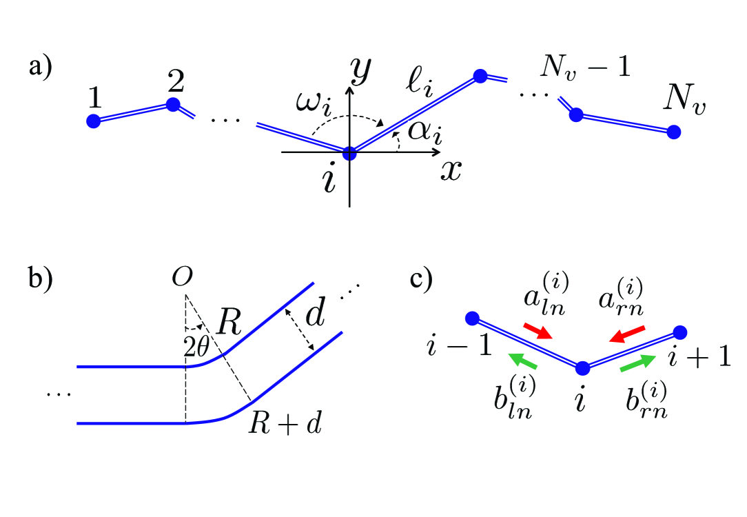
Figure 1: a) Sketch of a segmented 2D planar nanowire showing the definitions of the random angles $\alpha_{i}$ and $\omega_{i}$ for each vertex and the segment lengths $\ell_{i}$. b) Model of the vertex as a circular bend, with the definitions of the bend radius $R$ and angle $2\theta$. c) Notation for the scattering amplitudes for left and right incidence on vertex $i$.

II Segmented wire model

II.1 Model definition

We consider a quantum waveguide formed by joining straight 2D channels of width $d$. The joining vertices are described by simple circular bends of radius $R$ and angle $2\theta$. Figure 1 sketches the system definitions. A set of values $\{\ell_{i},\alpha_{i},R_{i},i=1,\dots,N_{v}\}$, with $N_{v}$ the number of vertices, gives a particular physical realization of the segmented wire. We are interested in the statistical properties when these values vary randomly within given intervals

$$\alpha_{i} \in [-\alpha_{0},\alpha_{0}]\;,$$ (1)

$$\ell_{i} \in [\ell_{0}(1-p_{\ell}),\ell_{0}(1+p_{\ell})]\;,$$ (2)

$$R_{i} \in [R_{0}(1-p_{R}),R_{0}(1+p_{R})]\;,$$ (3)

where $\alpha_{0}$, $\ell_{0}$, $R_{0}$, $p_{\ell}$ and $p_{R}$ characterize the parameter ranges of random variation. The parameters $p_{\ell}$ and $p_{R}$ are dimensionless and fulfill $0\leq p_{\ell,R}\leq 1$. They represent the maximum random variation (in relative terms) of the segment lengths around $\ell_{0}$ and of the vertex radius around $R_{0}$, respectively.

II.2 The transport problem

Each vertex is characterized by a scattering matrix relating input and output wave amplitudes

$$\left(\begin{array}[]{c}b_{l}^{(i)}\\ b_{r}^{(i)}\end{array}\right)=\left(\begin{array}[]{cc}r^{(i)}&t^{(i)}\\ t^{(i)}&r^{(i)}\end{array}\right)\left(\begin{array}[]{c}a_{l}^{(i)}\\ a_{r}^{(i)}\end{array}\right)\;,$$ (4)

where the notation of Fig. 1c is used. For the case of multiple propagating modes, input and output amplitudes in Eq. (4) correspond to vectors. For instance, $a^{(i)}_{l}\equiv(a^{(i)}_{l1},a^{(i)}_{l2},\dots,a^{(i)}_{lN_{p}})$, with $N_{p}$ the total number of propagating modes. Analogously, the transmission and reflection coefficients become matrices, $t^{(i)}\equiv t^{(i)}_{nn^{\prime}}$, $r^{(i)}\equiv r^{(i)}_{nn^{\prime}}$ with $n,n^{\prime}=1,\dots,N_{p}$.

There is a relation between input and output amplitudes for successive vertices. For instance, right-output from vertex $i-1$ in mode $n$ coincides with left-input for vertex $i$, with a phase, i.e., $b^{(i-1)}_{rn}=a^{(i)}_{ln}\exp{(-ik_{n}l_{i-1})}$. A closed system of linear equations is obtained assuming unit left incidence on vertex 1 in mode $n_{i}$. The linear system of $4N_{p}N_{v}$ equations reads

$$\begin{array}[]{rcll}\rule{0.0pt}{0.0pt}a^{(i)}_{ln}&=&\delta_{n,n_{i}}&(i=1)\;,\\ \rule{0.0pt}{15.6491pt}a^{(i)}_{rn}&=&0&(i=N_{v})\;,\\ \rule{0.0pt}{15.6491pt}b^{(i)}_{ln}-a^{(i-1)}_{rn}\exp{(-ik_{n}l_{i-1})}&=&0&(i\neq 1)\;,\\ \rule{0.0pt}{15.6491pt}b^{(i)}_{rn}-a^{(i+1)}_{ln}\exp{(-ik_{n}l_{i})}&=&0&(i\neq N_{v})\;,\\ \rule{0.0pt}{15.6491pt}b^{(i)}_{ln}-\sum_{n^{\prime}}{r^{(i)}_{nn^{\prime}}a^{(i)}_{ln^{\prime}}}-\sum_{n^{\prime}}{t^{(i)}_{nn^{\prime}}a^{(i)}_{rn^{\prime}}}&=&0&(i=1,\dots,N_{v})\;,\\ \rule{0.0pt}{15.6491pt}b^{(i)}_{rn}-\sum_{n^{\prime}}{t^{(i)}_{nn^{\prime}}a^{(i)}_{ln^{\prime}}}-\sum_{n^{\prime}}{r^{(i)}_{nn^{\prime}}a^{(i)}_{rn^{\prime}}}&=&0&(i=1,\dots,N_{v})\;,\end{array}$$ (5)

where $n$ and $n^{\prime}$ are mode indexes ranging from 1 to $N_{p}$. The solution of the linear system yields the output amplitudes on each vertex as a function of the incidence mode $n_{i}$, $b^{(i)}_{rn}(n_{i})$. The total transmission is obtained by adding the modulus squared of the right-output amplitudes on the last vertex $N_{v}$ as

$$T=\sum_{n_{i}n_{o}}{\left|b^{(N_{v})}_{rn_{o}}(n_{i})\right|^{2}}\;.$$ (6)

Once the scattering matrices are known, the linear system can be efficiently solved in a numerical way for quite large values of the number of segments $N_{v}$. The computer solution is also fast enough to allow for an statistical analysis with the random variation of the parameters (Fig. 1a).

II.3 Vertex scattering matrix

The transmission and reflection matrices, $t$ and $r$, for a single vertex are a required input of the model. We describe each vertex as a circular bend of the 2D wire (Fig. 1b), a problem that was studied in Refs. Wu et al. (1992); Sprung et al. (1992); Sols and Macucci (1990); Lent (1990). In particular, we have followed the approach of Ref. Sols and Macucci (1990) that relies on the separability of Schrödinger’s equation in the bend region in radial and angular parts. Using polar coordinates for the bend region of Fig. 1b, with $\rho$ the distance to $O$ and $\phi$ the azimuthal angle, the wave function may be factorized as $P_{|\nu|}(\rho)\exp{(\pm|\nu|\phi)}$. The eigenvalue problem given in Eq. (2b) of Ref. Sols and Macucci (1990) determines both $\nu^{2}$ and $P_{|\nu|}(\rho)$. For completeness, we repeat here this eigenvalue problem

$$\rho^{2}\frac{d^{2}P_{|\nu|}(\rho)}{d\rho^{2}}+\rho\frac{dP_{|\nu|}(\rho)}{d\rho} + \frac{2mE}{\hbar^{2}}\rho^{2}P_{|\nu|}(\rho)=$$ (7)

$$- \nu^{2}P_{|\nu|}(\rho)\;.$$

Equation (7) is not apparently Hermitian. However, the transformation $P_{|\nu|}=\sqrt{\rho}F_{|\nu|}$ leads to

$$\rho\frac{d^{2}}{d\rho^{2}}\rho\,F_{|\nu|}(\rho)+\left(\frac{1}{4}+\frac{2mE}{\hbar^{2}}\rho^{2}\right)F_{|\nu|}(\rho)=-\nu^{2}F_{|\nu|}(\rho)\;,$$ (8)

that, being Hermitian, can be numerically diagonalized with standard routines for symmetric matrices. As $\nu^{2}$ is thus a real value, $\nu$ can be either real or purely imaginary, which describe evanescent and propagating angular waves in the bend, respectively. Determining this way the bend modes, the matching conditions at the interfaces (dashed lines of Fig. 1b) yield the required scattering matrices. As mentioned in Ref. Sols and Macucci (1990), truncating the number of bend modes and straight wire modes to the same value, a linear system of equations replaces the matching conditions. We have implemented that method and checked that our solution reproduces the transmission and reflection probabilities given in Ref. Sols and Macucci (1990).

At low energies it was shown in Ref. Sprung et al. (1992) that the circular bend may be approximated by a 1D square well of depth $V_{0}=\hbar^{2}/(2m\bar{R}^{2})$ and width $2a=2\bar{R}\theta$, where $\bar{R}=\sqrt{R(R+d)}$ is an average effective radius. In this approximation the scattering matrices are, of course, analytical.

III Localization properties

The localization length $\ell_{\it loc}$ is a characteristic distance such that random segmented wires whose total length $L$ fulfills $L>>\ell_{\it loc}$ present a statistical distribution of $\log(T)$ that is Gaussian (normal) distributed around a mean value. Of course, the localization length depends on the system parameters as well as on the energy $E$ of the transport electrons. Deeply in the localized regime ($L>>\ell_{\it loc}$) the transmission is in general greatly quenched for the huge majority of system realizations. It is therefore very relevant to characterize the parameter dependence of the localization length, as this is crucial for the electrical properties in coherent transport through the system.

In shorter wires ($L<\ell_{\it loc}$) transport is diffusive and typical of metallic conductors characterized by Ohm’s law. In this case there is a linear relation between the electrical resistance and total length $L$. That is, in our model, we may expect a regime such that

$$\left\langle\frac{1}{T}\right\rangle=\frac{1}{N_{p}}+\frac{1}{N_{p}\ell_{\Omega}}\langle L\rangle\;,$$ (9)

where the averages are regarding system realizations and we have defined a diffusive (ohmic) length $\ell_{\Omega}$ that characterizes the electron mean free path. The constant contribution $1/N_{p}$ ($N_{p}$ number of propagating modes) in Eq. (9) represents the contact resistance, present even without any scattering effect. Localization length and mean free path are actually related by $\ell_{\it loc}\approx N_{p}\ell_{\Omega}$, relation that we have explicitly checked for segmented wires (see also Ref. García-Martín et al. (1997)). For completeness, besides the localized and diffusive regimes the so-called ballistic regime corresponds to $L<<\ell_{\Omega}$, such that only the contact resistance contribution matters in Eq. (9).

Yet another characteristic length may be obtained using a semiclassical approximation. In a semiclassical description the scatterers representing the vertices add up their effects incoherently, yielding a total transmission $T_{sc}$ that is independent of the segments length $\ell_{0}$,

$$\frac{1}{T_{sc}}-\frac{1}{N_{p}}=\sum_{i=1}^{N_{v}}\left(\frac{1}{T^{(i)}}-\frac{1}{N_{p}}\right)\;,$$ (10)

where $T^{(i)}\equiv|t^{(i)}|^{2}$ is the transmission probability corresponding to vertex $i$. As the mean total length is $\langle L\rangle\approx N_{v}\ell_{0}$, Eq. (10) yields an ohmic scaling similar to Eq. (9),

$$\frac{1}{T_{sc}}=\frac{1}{N_{p}}+\frac{1}{\ell_{sc}}\langle L\rangle\;,$$ (11)

where we defined a semiclassical length

$$\ell_{sc}=\frac{\ell_{0}}{\left(\frac{1}{N_{v}}\sum_{i}{\frac{1}{T^{(i)}}}\right)-\frac{1}{N_{p}}}\;.$$ (12)

As shown below, $\ell_{sc}$ yields an estimate of $\ell_{\it loc}$ that averages all possible oscillations and resonances due to quantum interference.

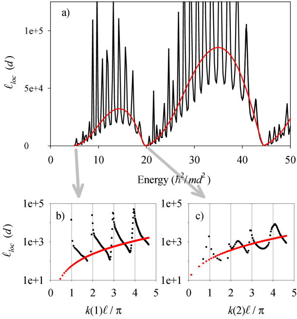
Figure 2: Localization length as a function of energy. The lower panels show the dependence on mode wave number for the energy ranges around the first and second onsets for mode activation. The red line is the semiclassical result $\ell_{sc}$ defined in Eq. (12). Parameters: $\ell_{0}=10d$, $R_{0}=0.2d$, $p_{\ell}=0.01$, $p_{R}=0.01$, $\alpha_{0}=60^{\circ}$.

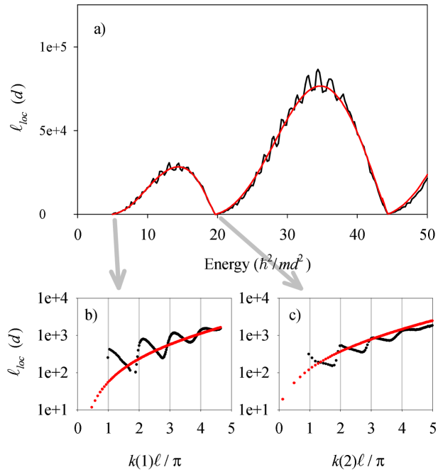
Figure 3: Same as Fig. 2 but with $p_{\ell}=0.1$.

The ohmic regime is sometimes referred to as diffusive or metallic and it is characterized by a relatively low transmission, as compared to the maximum value allowed by the conductance quantization of the channel. Within the random matrix theory this is a regime of universal conductance fluctuations Beenakker (1997), the transmission being normally distributed with a statistical dispersion $\Delta T=\sqrt{2/15}$ (in systems with time reversal symmetry like ours). On the other hand, in the ballistic limit the transmission reaches the quantized maximum values allowed by the number of propagating modes $N_{p}$. We expect this regime only in short-enough wires and relatively high energies, such that scattering effects become negligible.

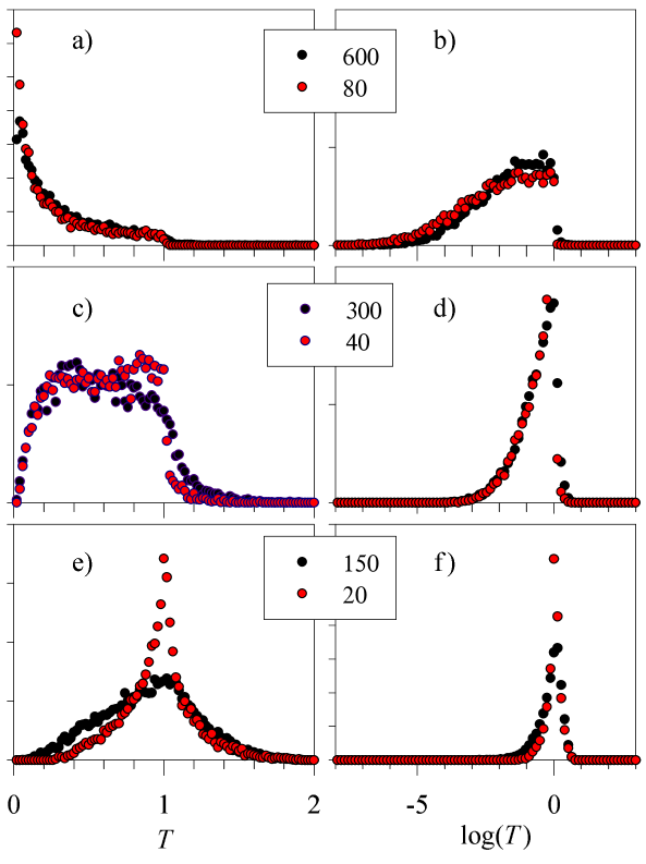
Figure 4: Probability distribution of $T$ (left) and $\log(T)$ (right) in the crossover regime. The number of segments corresponding to each symbol varies in each panel as indicated. Black circles correspond to an energy $E=19.8\hbar^{2}/md^{2}$ for which the localization length is $\ell_{\it loc}\approx 3000d$. On the other hand, red circles correspond to $E=20.1\hbar^{2}/md^{2}$ and $\ell_{\it loc}\approx 280d$. The rest of parameters are as in Fig. 2.

IV Results

Figure 2 shows the energy dependence of $\ell_{\it loc}$ in a segmented wire. A conspicuous resonant behavior is seen, with closely lying spikes and an overall beating pattern corresponding to the successive activation of propagating modes. The beating is accurately reproduced by the semiclassical length $\ell_{sc}$ (red line) that nicely averages the resonant oscillations. The resonances occur when an integer number of wave lengths fit in the segment length $\ell_{0}$, i.e., $k(i)\ell_{0}=n\pi$, with $n$ an integer. This resonant condition does not depend on the vertex parameters $\alpha$, $R_{0}$, neither on $p_{R}$, but it quickly degrades when $p_{\ell}$ increases, as seen in Fig. 3. As shown in this figure, a dispersion of $\pm 10\%$ is enough to greatly reduce the resonance peaks. The resonant behavior with one propagating mode is qualitatively similar to the behavior in strictly 1D systems discussed in Refs. Herrera-González et al. (2013); Díaz et al. (2015). We stress, however, that we also find similar resonances in higher energy regions, where more modes become propagating.

The crossover between diffusive and localized regimes of disordered wires is known to be characterized by a nontrivial evolution of the $T$ and $\log(T)$ distributions Muttalib and Wölfle (1999); García-Martín and Sáenz (2001); Gopar et al. (2002); Alcázar-López and Méndez-Bermúdez (2013). We have explored whether the crossover is greatly affected by the resonant condition or not. More specifically, we choose parameter sets corresponding to a maximum and a minimum in localization length and check the evolution with varying number of segments. Figure 4 shows that even when the localization length changes by more than an order of magnitude with a small energy change (spiking behavior in Fig. 2), the qualitative evolution of the probability distributions is very similar.

The results of Fig. 4a,b correspond to $L\approx 2\ell_{\it loc}$, just entering the localized regime. They show a long-tail $T$ distribution with a change of behavior at $T=1$. On the other hand, $\log(T)$ is given by an asymmetric Gaussian in this region. The central panels, Figs. 4c,d correspond to the middle of the crossover with $L\approx\ell_{\it loc}$ and show a rather flat distribution of transmissions with a dip at $T\approx 0$ Wang et al. (1998); Plerou and Wang (1998). The lower panels Figs. 4e,f signal the beginning of the diffusive regime $L\approx 0.5\ell_{\it loc}$ and show a kink at $T=1$ separating two regions in the $T$-distribution. These crossover features are already known and they agree well with the results of studies of disordered wires Muttalib and Wölfle (1999); García-Martín and Sáenz (2001); Gopar et al. (2002). They are, nevertheless, shown here to stress the similar evolution for widely different localization lengths due to resonance. It is worth mentioning that when the localization length is very short, as for the red dots in Fig. 4, the transition from quasi-ballistic to localized is more abrupt, leaving a quite reduced diffusive range. We attribute to this enhanced quasi-ballistic behavior the increased kink at $T\approx 1$ of the red dots in Fig. 4e, as compared with the black ones.

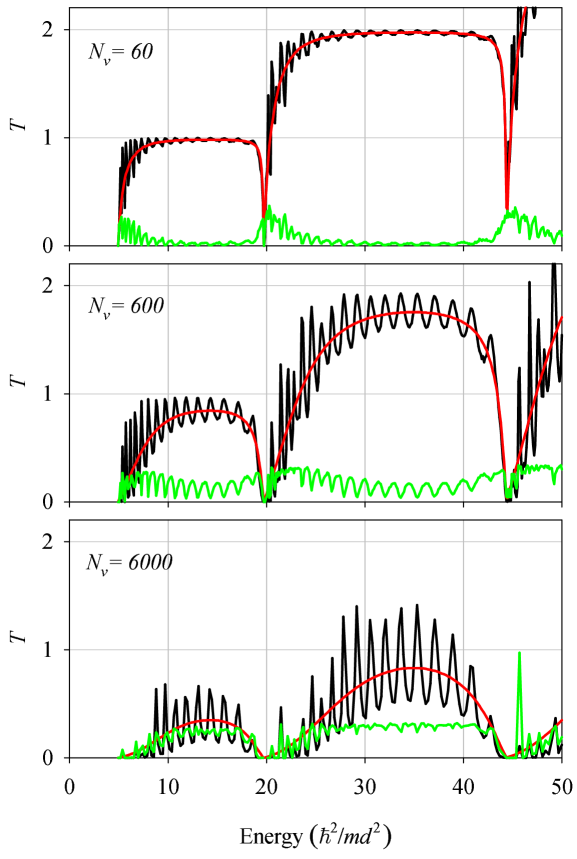
Figure 5: Mean conductance as a function of energy for increasing number of segments as indicated in each panel. The same parameters of Fig. 2 have been used. The green line shows the dispersion of the statistical distribution of transmissions while the red line is the semiclassical result $T_{sc}$.

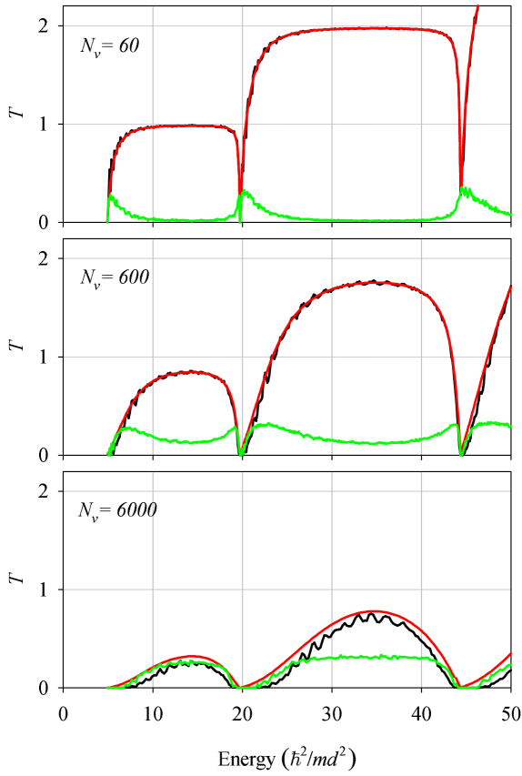
Figure 6: Same as Fig. 5 but with $p_{\ell}=0.1$.

We discuss next the mean conductance of a wire with a fixed number of segments (Figs. 5 and 6). The conductance shows a general tendency to increase in discrete steps as the energy increases, typical of quantum wires. The conductance plateaus, however, are distorted in remarkable ways. First we notice in Fig. 5 the already mentioned resonant oscillations, present at the beginning of each plateau for the smaller $N_{v}$ and eventually extending to all the plateau for the larger $N_{v}$’s. A pronounced conductance dip is also observed at the beginning of each plateau. For the shorter wires the plateaus saturate at the quantized values, while in the longer ones there is no clear saturation and the transmission is in general much lower than the corresponding quantized values.

The physics implied by Fig. 5 can be understood as a typical evolution of a finite-wire conductance with increasing energy: from a localized regime near the plateau onset, to an ohmic (diffusive) regime and eventually reaching a ballistic regime if the wire is short enough. The localized regime occurs at the plateau onset, where the localization length is small (Figs. 2 and 3). As the energy increases, an ohmic regime is reached, characterized by a sizeable dispersion of the transmissions and by the linearity of the inverse transmission with length. In short wires (Fig. 5 upper panel) the system may also reach the quantum ballistic regime, with a quantized unitary transmission and vanishing dispersion.

As with the localization lengths, the strong transmission oscillations due to wave number quantization are quenched if the segment lengths vary by a sizeable amount. Figure 6 shows the transmission with $p_{\ell}=0.1$. In this case, there is a better correspondence with the semiclassical result.

V Conclusions

A model of random segmented 2D wire with circular bends has been presented. We focussed on the scattering induced by the bends and how this leads to the emergence of localization. A strong resonant behavior is predicted when the segments are all of very similar lengths. A spiking behavior of the localization length is found, not only with a single propagating mode, but also in presence of several modes. A beating pattern of the spiking is accurately reproduced by a semiclassical model, averaging quantum oscillations and resonances. The localization resonances are reduced when the distribution of segment lengths gets broader.

The localized-diffusive crossover is shown to agree with the known behaviors from disordered wires. The same qualitative evolution of the $T$ and $\log(T)$ distributions is found for large and small localization lengths, moving across the resonance spikes. For short localization lengths the diffusive regime is much reduced, yielding a more abrupt evolution from ballistic to localized cases. A fixed-length wire typically evolves with increasing energy from localization at the beginning of each transmission plateau, to a diffusive regime and to ballistic behavior towards the plateau end. The ballistic regime may be reached only if the wire is short enough.