Optimization approach for the simultaneous reconstruction of the dielectric permittivity and magnetic permeability functions from limited observations

Abstract

We consider the inverse problem of the simultaneous reconstruction of the dielectric permittivity and magnetic permeability functions of the Maxwell’s system in 3D with limited boundary observations of the electric field. The theoretical stability for the problem is provided by the Carleman estimates. For the numerical computations the problem is formulated as an optimization problem and hybrid finite element/difference method is used to solve the parameter identification problem.

1 Introduction

This paper is focused on the numerical reconstruction of the dielectric permittivity coefficient $\varepsilon(x)$ and the magnetic permeability coefficient $\mu(x)$ for Maxwell’s system basing our observation on a single measurement data of the electric field $E(x,t)$. That means that we use boundary measurements of $E(x,t)$ which are generated by a single direction of a plane wave. For the numerical reconstructions of the dielectric permittivity coefficient $\varepsilon(x)$ and the magnetic permeability coefficient $\mu(x)$, we consider a similar hybrid finite element/difference method (FE/FDM) as was developed in [3].

In the literature, the stability results for Maxwell’s equations have been proposed by Dirichlet-to-Neumann map or by Carleman estimates. For results using Dirichlet-to-Neu-mann map with infinitely many boundary observations, see [9, 12, 13, 31, 41, 46]. For results with a finite number of observations several Carleman estimates have been derived in [10, 21, 30, 34, 35, 36]. In order to solve the coefficient inverse problem of Maxwell’s equations numerically, we consider only those theoretical results that involve finite number of observations.

Since real observations are generally corrupted by noise, it is important to verify whether close observations lead to close estimations of the coefficients. The results of this paper give such conditions on the observations for estimating the parameters $\mu(x)$ and $\varepsilon(x)$ of the Maxwell’s system (1) from the observations of $E(x,t)$ on the boundary of the domain. In particular, we obtain a stability inequality of the form

$$\|(\mu_{1},\varepsilon_{1})-(\mu_{2},\varepsilon_{2})\|\leq f\left(\,\|\hbox{Observation}(E_{1})-\hbox{Observation}(E_{2})\|\right)$$

$$\mbox{for }f(s)\mbox{ such that }\displaystyle\lim_{s\rightarrow 0}f(s)=0,$$

which links the distance between two sets of coefficients with the distance between two sets of boundary observations of the electric field $E(x,t)$. Such stability inequalities lead to the uniqueness of the coefficients $(\mu(x),\varepsilon(x))$ given the observation $"\hbox{Observation}(E(x,t))"$ on a small neighborhood of the boundary of the domain of interest. They are also useful for the numerical reconstruction of the coefficients using noise-free observations [27]. Our main theoretical result concerns stability inequality which gives an estimate of the norm of two coefficients $\varepsilon$ and $\mu$ in terms of observation of only the electric field $E(x,t)$ on the boundary of the domain. This implies directly a uniqueness result. In the domain of the inverse problems, associated to reconstructing the Maxwell’s coefficients from finite number of observations, except the reference [30], and up to our knowledge, there exists no result involving only one component $E(x,t)$ (or the component $H(x,t)$).

In this work, the minimization problem of reconstructing functions $\varepsilon(x)$ and $\mu(x)$ is reformulated as the problem of finding a stationary point of a Lagrangian involving a forward equation (the state equation), a backward equation (the adjoint equation) and two equations expressing that the gradients with respect to the coefficients $\varepsilon(x)$ and $\mu(x)$ vanish. Moreover, in our work the forward and adjoint problems are given by time-dependent Maxwell’s equations for the electric field. This means that we have observations of the electric field in space and in time which provides us better reconstruction of both coefficients. In order to get the computed values of $\varepsilon(x)$ and $\mu(x)$, we arrange an iterative process by solving in each step the forward and backward equations and updating the coefficients $\varepsilon(x)$ and $\mu(x)$ at every step of our iterations.

Recall, that in our optimization procedure the forward and adjoint problems are given by the time-dependent Maxwell’s system for the electric field. For the numerical solution of the Maxwell equations, different formulations are available. One can consider, for example, the edge elements of Nédélec [40], the node-based first-order formulation of Lee and Madsen [33], the node-based curl-curl formulation with divergence condition of Paulsen and Lynch [42] or the interior-penalty discontinuous Galerkin FEM [26]. In this work, for the discretization of the Maxwell’s equations, we use stabilized domain decomposition method of [3] with divergence condition of Paulsen and Lynch [42] which removes spurious solutions when local mesh refinement is applied and material discontinuities are not too big [5]. Numerical tests of [3] in the case of coefficient inverse problems (CIPs), similar to our of recent experimental work [7], show that these spurious solutions will not appear.

It is well known that edge elements are the most satisfactory from a theoretical point of view  [37] since they automatically satisfy the divergence free condition. However, in the case of time-dependent computations they are less attractive. First, they are time consuming because the solution of a resulted linear system is required at every time iteration. Second, in [22] was shown that in the case of triangular or tetrahedral edge elements, the entries of the diagonal matrix resulting from mass-lumping are not necessarily strictly positive, and thus, explicit time stepping cannot be used in general. The method of [3] where nodal elements were used leads to a fully explicit and efficient scheme when mass-lumping is applied [29, 22]. This method is efficiently implemented in the software package WavES [51] in C++ using PETSc [43] and MPI (message passing interface) and is convenient for our simulations.

We note, that we reconstruct functions $\varepsilon(x)$ and $\mu(x)$ simultaneously. Up to our knowledge, there are few studies (e.g. [25]) that consider the simultaneous recovery of $\varepsilon(x)$ and $\mu(x)$ within the spatio-temporal Maxwell’s equations. In the papers [7, 3], which use the same optimization approach, the coefficient $\mu$ is assumed to have a known and a constant value, i.e. $\mu=1$, which means that the medium is non-magnetic. However, it is well known that in many situations, we need to deal with magnetic materials (e.g. metamaterials [48], low-loss materials [45]).

Potential applications of our algorithm are in reconstructing the electromagnetic parameters in nanocomposites or artificial materials [45, 47, 48], imaging of defects and their sizes in a non-destructive testing of materials and in photonic crystals [15], measurement of the moisture content [14] and drying processes [38], for example.

Our numerical simulations show that we are able to accurately reconstruct simultaneously contrasts for both functions $\varepsilon(x)$ and $\mu(x)$ as well as their locations. In our future work, similarly with [7, 3, 6], we are planning also to reconstruct shapes of the inclusions using a posteriori error estimates in the Tikhonov functional or in the reconstructed coefficients and based on them an adaptive finite element method.

The paper is organized as follows. In Section 2 we state the theoretical results of recovering $\varepsilon(x)$ and $\mu(x)$ from the limited boundary measurements of $E(x,t)$. Section 3 is devoted to presenting the numerical method used in this article. In Section 4, we give detailed information about our discrete numerical method and we outline the algorithm for the solution of our inverse problem. The numerical results are presented in Section 5. Discussions and conclusions are given in Section 6.

2 Theoretical results

Let us consider a bounded domain $\Omega\subset\mathbb{R}^{3}$ with a smooth boundary $\partial\Omega$, and define by $\Omega_{T}:=\Omega\times(0,T)$, $\partial\Omega_{T}:=\partial\Omega\times(0,T)$, where $T$ is a strictly positive constant. The electromagnetic equations in an inhomogeneous isotropic case in the bounded domain $\Omega\subset\mathbb{R}^{d},~{}d=2,3$ with boundary $\partial\Omega$, are described by the first order system of partial differential equations

$$\left\{\begin{array}[]{llllll}\partial_{t}D-\nabla\times H(x,t)=0&&\mbox{ in }\Omega_{T}\\ \partial_{t}B+\nabla\times E(x,t)=0,&&\mbox{ in }\Omega_{T},\\ D(x,t)=\varepsilon E(x,t),\quad B(x,t)=\mu H(x,t),&&\\ E(x,0)=E_{0}(x),\quad H(x,0)=H_{0}(x),&&\\ \nabla\cdot D(x,t)=0,\quad\nabla\cdot B(x,t)=0,&&\mbox{ in }\Omega_{T},\\ D(x,t)\times\nu=0,\quad B(x,t)\cdot\nu=0,&&\textrm{on }\,\partial\Omega_{T},\end{array}\right.$$ (1)

where $E(x,t),H(x,t),D(x,t),B(x,t)$ are three-dimensional vector-valued functions of the time $t$ and the space variable $x=(x_{1},x_{2},x_{3})$, and correspond to the electric and magnetic fields and the electric and magnetic inductions, respectively. The dielectric permittivity, $\varepsilon(x)>0$ and the magnetic permeability, $\mu(x)>0$, depend on $x\in\Omega$, $\nu=\nu(x)$ denotes the unit outward normal vector to $\partial\Omega$.

Our goal is to reconstruct the coefficients $\varepsilon(x)$ and $\mu(x)$ in the system (1) with appropriate initial conditions $E_{0}$ and $H_{0}$ on the electric and magnetic inductions, using only a finite number of observations of the electric field $E(x,t)$ on the boundary $\partial\Omega$ of the domain $\Omega$.

We base our theoretical approach on the work [10]. In this work the authors obtained a stability inequality for the dielectric permittivity $\varepsilon(x)$ and the magnetic permeability $\mu(x)$ involving boundary observations of both magnetic induction $B(x,t)$ and electric induction $D(x,t)$ (see theorem 1 of [10]). With the same assumptions, as those in [10], we can reformulate this stability result using only the observations of the electric field $E(x,t)$ (or correspondingly, using only the observations of the magnetic field $H(x,t)$):

Assume that the functions $\mu(x)$ and $\varepsilon(x)$ in $\mathcal{C}^{2}(\overline{\Omega}),x\in\overline{\Omega}$ obey

$$\mu(x)\geq\mu_{0},\quad\varepsilon(x)\geq\varepsilon_{0},$$ (2)

for some $\varepsilon_{0}>0$ and $\mu_{0}>0$. Next, for simplicity, we introduce some similar notations to the ones introduced in [10].

Let us pick $x_{0}\in\mathbb{R}^{3}\backslash\overline{\Omega}$, set $c(x)=(\mu(x)\varepsilon(x))^{-1}$ for $x\in\overline{\Omega}$, $c_{0}=(\mu_{0}\varepsilon_{0})^{-1}$ and assume that the following condition holds for some $\rho\in(0,c_{0})$

$$\frac{3}{2}\left|\nabla\log c(x)\right|\left|x-x_{0}\right|\leq 1-\frac{\rho}{c_{0}},\quad x\in\overline{\Omega}.$$ (3)

This technical condition is claimed by the weight function $\psi_{0}=|x-x_{0}|^{2}$ that is used to create the Carleman estimate established to prove the theorem 2.1 in [10]. In other terms, (3) arises from the classical pseudo-convexity condition. Another standard hypothesis is that the coefficients $\varepsilon$ and $\mu$ are known in a neighborhood of the boundary of $\Omega$

Next, we define $\omega=\Omega\cap\mathcal{O}$ where $\mathcal{O}$ is some neighborhood of $\partial\Omega$ in $\mathbb{R}^{3}$. Further let $M_{0}>0$ and two given functions $\mu^{\sharp},\lambda^{\sharp}$ belong to $\mathcal{C}^{2}(\omega)$. Now we can define the admissible set of unknown coefficients $\mu$ and $\varepsilon$ as

$$\Lambda_{\omega}(M_{0})=\left\{(\mu,\varepsilon)\ \textrm{verifying}\,(\ref{1.2});\left\|(\mu,\varepsilon)\right\|_{\mathcal{C}^{2}(\overline{\Omega})}\leq M_{0}\ \textrm{and}\,(\mu,\varepsilon)=(\mu^{\sharp},\varepsilon^{\sharp})\ \textrm{in}\ \omega\right\}.$$ (4)

We set

$$\mathcal{V}=H_{\tau,0}(\textrm{curl\,},\textrm{div\,}0;\Omega)\times{\rm H}_{n,0}(\textrm{curl\,},\textrm{div\,}0;\Omega),$$

where

$$H_{*,0}(\textrm{curl\,},\textrm{div\,}0;\Omega)=\{u\in H^{1}(\Omega)^{3},\ \textrm{div\,}u=0\ {\rm and}\ \gamma_{*}u=0\},\ *=\tau,n.$$

Further, for the identification of $(\mu,\varepsilon)$, imposing (as will appear in the sequel) that $(B(x,t),D(x,t))$ are observed twice, we consider two sets of initial data $(D_{0}^{k},B_{0}^{k})$, $k=1,2$ such that,

$$\mathrm{D}_{0}^{k}(x)=\left(d_{1}^{k}(x),d_{2}^{k}(x),d_{3}^{k}(x)\right)^{\top},\quad\mathrm{B}_{0}^{k}(x)=\left(b_{1}^{k}(x),b_{2}^{k}(x),b_{3}^{k}(x)\right)^{\top},$$

and define the $12\times 6$ matrix

$$\mathcal{K}(x)=\left(\begin{array}[]{cccccc}e_{1}\times\mathrm{B}_{0}^{1}&e_{2}\times\mathrm{B}_{0}^{1}&e_{3}\times\mathrm{B}_{0}^{1}&0&0&0\\ 0&0&0&e_{1}\times\mathrm{D}_{0}^{1}&e_{2}\times\mathrm{D}_{0}^{1}&e_{3}\times\mathrm{D}_{0}^{1}\\ e_{1}\times\mathrm{B}_{0}^{2}&e_{2}\times\mathrm{B}_{0}^{2}&e_{3}\times\mathrm{B}_{0}^{2}&0&0&0\\ 0&0&0&e_{1}\times\mathrm{D}_{0}^{2}&e_{2}\times\mathrm{D}_{0}^{2}&e_{3}\times\mathrm{D}_{0}^{2}\\ \end{array}\right),$$ (5)

where $x\in\Omega$. Then we can write that $(\mathrm{B}_{i}^{k}(x,t),\mathrm{D}_{i}^{k}(x,t))$ are the solution to (1) with the initial data $(\mathrm{B}_{0}^{k},\mathrm{D}_{0}^{k})$, $k=1,2$, where $(\mu,\varepsilon)$ are substituted with $(\mu_{i},\varepsilon_{i})$, $i=1,2$.
Finally, we note that $\mathcal{H}(\Omega_{T})=H^{3}(-T,T;L^{2}(\Gamma))\cap H^{2}(-T,T;H^{1}(\Gamma))$ is a Hilbert space equipped with the norm

$$\left\|u\right\|^{2}_{\mathcal{H}(\Omega_{T})}=\left\|u\right\|^{2}_{H^{3}(-T,T;L^{2}(\Gamma))}+\left\|u\right\|^{2}_{H^{2}(-T,T;H^{1}(\Gamma))},\quad u\in\mathcal{H}(\Omega_{T}).$$

The extension of the time interval to (-T,T) corresponds to a technical point in the proof of the stability inequality (see lemma 3 in [10]).
Now we recall the main theoretical result of the paper [10]: Under some hypothesis on $T$ and choosing initial conditions $(\mathrm{B}_{0}^{k},\mathrm{D}_{0}^{k})$, $k=1,2$ verifying some additional assumptions, then there are two constants $C>0$ and $\kappa\in(0,1)$, depending on $\Omega$, $\omega$, $T$, $M$ and $M_{0}$, such that we have:

$$\left\|\mu_{1}-\mu_{2}\right\|_{H^{2}(\Omega)} + \left\|\varepsilon_{1}-\varepsilon_{2}\right\|_{H^{2}(\Omega)}$$

$$\leq C\left(\sum_{k=1}^{2}\left(\left\|\left(\mathrm{B}_{1}^{k}-\mathrm{B}_{2}^{k}\right)_{\tau}\right\|_{\mathcal{H}(\Omega_{T})}+\left\|\left(\mathrm{D}_{1}^{k}-\mathrm{D}_{2}^{k}\right)_{\nu}\right\|_{\mathcal{H}(\Omega_{T})}\right)\right)^{\kappa}.$$

Under the same assumptions and considering the definition of the electric induction $\mathrm{D}_{i}$ and the magnetic induction $\mathrm{B}_{i}$ for $i=1,2$ we can write in the neighborhood $\omega$ of the boundary $\partial\Omega$ the following relations:

$$\partial_{t}B_{i}^{k}=-\textrm{curl\,}\varepsilon_{i}^{-1}\mathrm{D}_{i}^{k},\mbox{ in }\omega\times(-T,T),\mbox{ for }i=1,2\mbox{ and }k=1,2.$$

Since $\varepsilon_{i}=\varepsilon^{\sharp}$, for $i=1,2$ in $\omega$, we can write

$$\partial_{t}(\mathrm{B}^{k}_{1}-\mathrm{B}^{k}_{2})=-\textrm{curl\,}\frac{1}{\varepsilon^{\sharp}}(\mathrm{D}_{1}^{k}-\mathrm{D}_{2}^{k})\mbox{ in }\omega\times(-T,T),\mbox{ for }k=1,2.$$

It is straightforward to verify that

$$\partial_{t}(\mathrm{B}^{k}_{1}-\mathrm{B}^{k}_{2})=-\frac{1}{\varepsilon^{\sharp}}\textrm{curl\,}(\mathrm{D}_{1}^{k}-\mathrm{D}_{2}^{k})-\nabla\frac{1}{\varepsilon^{\sharp}}\times(\mathrm{D}_{1}^{k}-\mathrm{D}_{2}^{k}).$$

We define by

$$N(\partial\Omega_{T})=H^{3}(-T,T;L^{2}(\partial\Omega))\cap H^{2}(-T,T;H^{1}(\partial\Omega))\cap H^{1}(-T,T;H^{2}(\partial\Omega)),$$

the Hilbert space equipped with the norm

$$\left\|u\right\|^{2}_{N(\partial\Omega_{T})}=\left\|u\right\|^{2}_{H^{3}(-T,T;L^{2}(\partial\Omega))}+\left\|u\right\|^{2}_{H^{2}(-T,T;H^{1}(\partial\Omega))}+\left\|u\right\|^{2}_{H^{1}(-T,T;H^{2}(\partial\Omega))},\;$$

$u\in N(\partial\Omega_{T}).$Then from (4) and since $B_{1}^{k}(0,\cdot)=B_{2}^{k}(0,\cdot)$ and $D_{1}^{k}(0,\cdot)=D_{2}^{k}(0,\cdot)$, for $k=1,2$, we get

$$\left\|\mathrm{B}^{k}_{1}-\mathrm{B}^{k}_{2}\right\|_{\mathcal{H}(\Omega_{T})}\leq M_{0}\left\|\mathrm{D}^{k}_{1}-\mathrm{D}^{k}_{2}\right\|_{N(\partial\Omega_{T})}.$$

Thus we can deduce our theorem in the following form

Theorem 2.1

Let $T>c_{0}^{-1/2}\max_{x\in\overline{\Omega}}\left|x-x_{0}\right|$ and pick $(\mathrm{B}_{0}^{k},\mathrm{D}_{0}^{k})\in(H^{2}(\Omega)^{3}\times H^{2}(\Omega)^{3})\cap\mathcal{V}$, $k=1,2$, in such a way that there exists a $6\times 6$ minor $m(x)$ of the matrix $\mathcal{K}(x)$ defined in (5), obeying:

$$m(x)\neq 0,\ x\in\overline{\Omega\backslash\omega}.$$

Further, choose $(\mu_{i},\varepsilon_{i})\in\Lambda_{\omega}(M_{0})$, $i=1,2$, such that

$$\left\|\left(\mathrm{B}_{i}^{k},\mathrm{D}_{i}^{k}\right)\right\|_{\mathcal{C}^{3}(-T,T;W^{2,\infty}(\Omega))}\leq M,\ k=1,2,$$

for some $M>0$. Then there are two constants $C>0$ and $\kappa\in(0,1)$, depending on $\Omega$, $\omega$, $T$, $M$ and $M_{0}$, such that we have:

$$\left\|\mu_{1}-\mu_{2}\right\|_{H^{2}(\Omega)}+\left\|\varepsilon_{1}-\varepsilon_{2}\right\|_{H^{2}(\Omega)}\leq C\left({\sum_{k=1}^{2}{\left\|{D_{1}^{k}-D_{2}^{k}}_{\nu}\right\|_{N(\partial\Omega_{T})}}}\right)^{\kappa}.$$

3 Statement of the forward and inverse problems

3.1 The mathematical model

Below for any vector function $u\in\mathbb{R}^{3}$ our notations $u\in L^{2}(\Omega)$ or $u\in H^{k}(\Omega),k=1,2$, mean that every component of the vector function $u$ belongs to this space.

Next, we decompose $\Omega$ into two subregions, $\Omega_{\rm FEM}$ and $\Omega_{\rm FDM}$ such that $\Omega=\Omega_{\rm FEM}\cup\Omega_{\rm FDM}$, $\Omega_{\rm FEM}\cap\Omega_{\rm FDM}=\emptyset$ and $\partial\Omega_{\rm FEM}\subset\partial\Omega_{\rm FDM}$, for an illustration of the domain decomposition, see figure 1. In $\Omega_{\rm FEM}$ we use finite elements and in $\Omega_{\rm FDM}$ we will use finite difference method with first order absorbing boundary conditions [24]. The boundary $\partial\Omega$ is such that $\partial\Omega=\partial_{1}\Omega\cup\partial_{2}\Omega\cup\partial_{3}\Omega$ where $\partial_{1}\Omega$ and $\partial_{2}\Omega$ are, respectively, front and back sides of the domain $\Omega$, and $\partial_{3}\Omega$ is the union of left, right, top and bottom sides of this domain.

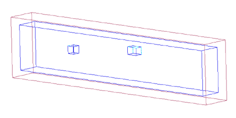
a) $\Omega=\Omega_{\rm FEM}\cup\Omega_{\rm FDM}$

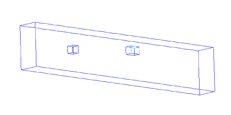
b) $\Omega_{\rm FEM}$

Figure 1: Illustration of the domain $\Omega$. a) Combination of domains $\Omega_{\rm FDM}$ and $\Omega_{\rm FEM}$. b) Only the domain $\Omega_{\rm FEM}$, with two inclusions.

By eliminating $B$ and $D$ from (1) we obtain the model problem for the electric field $E$ with the perfectly conducting boundary conditions at the boundary $\partial\Omega$ is as follows:

$$\varepsilon\frac{\partial^{2}E}{\partial t^{2}}+\nabla\times(\mu^{-1}\nabla\times E) = 0,~{}\mbox{in}~{}~{}\Omega_{T},$$ (6)

$$\nabla\cdot(\varepsilon E) = 0,~{}\mbox{in}~{}~{}\Omega_{T},$$ (7)

$$E(x,0)=f_{0}(x),~{}~{}~{}E_{t}(x,0) = f_{1}(x)~{}\mbox{in}~{}~{}\Omega,$$ (8)

$$E\times n = 0~{}\mbox{on}~{}~{}\partial\Omega_{T}.$$ (9)

Here we assume that

$$f_{0}\in H^{1}(\Omega),f_{1}\in L_{2}(\Omega).$$

We note that a similar equation can be derived also for $H$. For numerical solution of (6)-(9) in $\Omega_{\rm FDM}$ we use the finite difference method on a structured mesh with constant coefficients $\varepsilon=\varepsilon^{\sharp}\ =1$ and $\mu=\mu^{\sharp}=1$. In $\Omega_{\rm FEM}$, we use finite elements on a sequence of unstructured meshes $K_{h}=\{K\}$, with elements $K$ consisting of triangles in $\mathbb{R}^{2}$ and tetrahedra in $\mathbb{R}^{3}$ satisfying maximal angle condition [11].

In this work, for the discretization of the Maxwell’s equations we use stabilized domain decomposition method of [3] and consider Maxwell’s system in a convex geometry without reentrant corners where material discontinuities are not too big [5]. Since in our numerical simulations the relative permeability $\varepsilon$ and relative permittivity $\mu$ does not vary much, such assumptions about the coefficients are natural. Moreover, recent experimental works [7, 8, 49] show that material discontinuities in real applications of reconstruction of dielectrics (or refractive indices) of unknown targets placed in the air or ground using microwave imaging technology are not big. For application where the coefficients are assumed to be smooth see [20] and [52]. [20] considers breast imaging and [52] soil moisture imaging. In our work we treat discontinuities of coefficients $\epsilon$ and $\mu$ in a similar way as in formula (3.25) of section 3.5 in [17]. See also [4] for the case when only $\epsilon$ is unknown. Further, in our computations all materials with values of $\varepsilon>10$ are treated as metals and we call $\varepsilon$ as “apparent” or “effective” dielectric constant”, see [7, 8, 49] for more information and explanation.

To stabilize the finite element solution using standard piecewise continuous functions, we enforce the divergence condition (7) and add a Coulomb-type gauge condition [1, 39] to (6)-(9) with $0\leq s\leq 1$

$$\varepsilon\frac{\partial^{2}E}{\partial t^{2}}+\nabla\times(\mu^{-1}\nabla\times E)-s\nabla(\nabla\cdot(\varepsilon E)) = 0,~{}\mbox{in}~{}~{}\Omega_{T},$$ (10)

$$E(x,0)=f_{0}(x),~{}~{}~{}E_{t}(x,0) = f_{1}(x)~{}\mbox{in}~{}~{}\Omega,$$ (11)

$$E\times n = 0~{}~{}\partial\Omega_{T},$$ (12)

$$\mu(x)=\varepsilon\left(x\right) = 1\text{ in }\Omega_{\rm FDM}.$$ (13)

Let $S_{T}:=\partial_{1}\Omega\times(0,T)$ where $\partial_{1}\Omega$ is the backscattering side of the domain $\Omega$ with the time domain observations, and define by $S_{1,1}:=\partial_{1}\Omega\times(0,t_{1}]$, $S_{1,2}:=\partial_{1}\Omega\times(t_{1},T)$, $S_{2}:=\partial_{2}\Omega\times(0,T)$, $S_{3}:=\partial_{3}\Omega\times(0,T)$. Our forward problem used in computations, thus writes

$$\begin{split}\varepsilon\frac{\partial^{2}E}{\partial t^{2}}+\nabla\times(\mu^{-1}\nabla\times E)-s\nabla(\nabla\cdot(\varepsilon E))&=0,~{}\mbox{in}~{}~{}\Omega_{T},\\ E(x,0)=0,~{}~{}~{}E_{t}(x,0)&=0~{}\mbox{in}~{}~{}\Omega,\\ \partial_{n}E&=p\left(t\right),~{}\mbox{on}~{}S_{1,1},\\ \partial_{n}E&=-\partial_{t}E,~{}\mbox{on}~{}S_{1,2},\\ \partial_{n}E&=-\partial_{t}E,~{}\mbox{on}~{}S_{2},\\ \partial_{n}E&=0,~{}\mbox{on}~{}S_{3}.\\ \end{split}$$ (14)

We use the Neumann boundary conditions at the left and right hand sides of a domain $\Omega$ (recall, that $\Omega=\Omega_{\rm FEM}\cup\Omega_{\rm FDM}$ and in $\Omega_{\rm FDM}$ our coefficients $\varepsilon(x)=\mu(x)=1$) and first order absorbing boundary conditions [24] at the rest of the boundaries. Application of Neumann boundary conditions allows us to assume infinite structure in lateral directions and thus, allows us to consider the CIPs of the reconstruction of unknown parameters $\varepsilon$ and $\mu$ in a waveguide. Further, we assume homogeneous initial conditions.

It was demonstrated numerically in [3] that the solution of the problem (14) approximates well the solution of the original Maxwell’s equations for $\mu=1,s=1.$ The energy estimate of Theorem 4.1 of [3] implies an uniqueness result for the forward problem (14) with $\varepsilon\geq 1,\mu=1$. Similar theorem can be proven for the case when both coefficients are unknown, and it can be done in a future research.

We assume that our coefficients $\varepsilon\left(x\right),\mu(x)$ of equation (14) are such that

$$\begin{split}\varepsilon\left(x\right)&\in\left[1,d_{1}\right],~{}~{}d_{1}=const.>1,~{}\varepsilon(x)=1\text{ for }x\in\Omega_{\rm FDM},\\ \mu(x)&\in\left[1,d_{2}\right],~{}~{}d_{2}=const.>1,~{}\mu(x)=1\text{ for }x\in\Omega_{\rm FDM},\\ \varepsilon\left(x\right),\mu(x)&\in C^{2}\left(\mathbb{R}^{3}\right).\end{split}$$ (15)

The values of constants $d_{1},d_{2}$ in (15) are chosen from real life experiments similarly with [7, 8, 48, 49] and we assume that we know them a priori.

We consider the following

Inverse Problem (IP) Suppose that the coefficients $\varepsilon\left(x\right)$ and $\mu(x)$  satisfies (15) such that numbers $d_{1},d_{2}>1$ are given. Assume that the functions $\varepsilon\left(x\right),\mu(x)$ are unknown in the domain $\Omega\backslash\Omega_{\rm FDM}$. Determine the functions $\varepsilon\left(x\right),\mu(x)$ for $x\in\Omega\backslash\Omega_{\rm FDM},$  assuming that the following function $\tilde{E}\left(x,t\right)$ is known

$$E\left(x,t\right)=\tilde{E}\left(x,t\right),\forall\left(x,t\right)\in S_{T}.$$

A priori knowledge of an upper and lower bounds of functions $\varepsilon\left(x\right)$ and $\mu(x)$ corresponds well with the inverse problems concept about the availability of a priori information for an ill-posed problem [2, 23, 50]. In applications, the assumption $\varepsilon\left(x\right)=\mu(x)=1$ for $x\in\Omega_{\rm FDM}$ means that the functions $\varepsilon\left(x\right)$ and $\mu(x)$ have a known constant value outside of the medium of interest $\Omega\backslash\Omega_{\rm FDM}.$ The function $\tilde{E}\left(x,t\right)$ models time dependent measurements of the electric wave field at the backscattering boundary $\partial_{1}\Omega$ of the domain of interest. In practice, measurements are performed on a number of detectors, see [8, 49].

3.2 Optimization method

We reformulate our inverse problem as an optimization problem, where we seek for two functions, the permittivity $\varepsilon(x)$ and permeability $\mu(x)$, which result in a solution of equations (14) with best fit to time and space domain observations $\tilde{E}$, measured at a finite number of observation points on $\partial_{1}\Omega$. Our goal is to minimize the Tikhonov functional

$$F(E,\varepsilon,\mu)=\frac{1}{2}\int_{S_{T}}(E-\tilde{E})^{2}z_{\delta}(t)d\sigma dt+\frac{1}{2}\gamma_{1}\int_{\Omega}(\varepsilon-\varepsilon_{0})^{2}~{}~{}dx+\frac{1}{2}\gamma_{2}\int_{\Omega}(\mu-\mu_{0})^{2}~{}~{}dx,$$ (16)

where $\tilde{E}$ is the observed electric field, $E$ satisfies the equations (14) and thus depends on $\varepsilon$ and $\mu$, $\varepsilon_{0}$ is the initial guess for $\varepsilon$ and $\mu_{0}$ is the initial guess for $\mu$, and $\gamma_{i},i=1,2$ are the regularization parameters. Here $z_{\delta}(t)$ is a cut-off function, which is introduced to ensure that the compatibility conditions at $\overline{\Omega}_{T}\cap\left\{t=T\right\}$ for the adjoint problem (22) are satisfied, and $\delta>0$ is a small number. We choose a function $z_{\delta}$ such that

$$z_{\delta}\in C^{\infty}\left[0,T\right],\text{ }z_{\delta}\left(t\right)=\left\{\begin{array}[]{ll}1&\text{ for }t\in\left[0,T-\delta\right],\\ 0&\text{ for }t\in\left(T-\frac{\delta}{2},T\right],\\ 0<z_{\delta}<1&\text{ for }t\in\left(T-\delta,T-\frac{\delta}{2}\right).\end{array}\right.$$

Next, we introduce the following spaces of real valued vector functions

$$\begin{split}H_{E}^{1}&:=\{w\in H^{1}(\Omega_{T}):w(\cdot,0)=0\},\\ H_{\lambda}^{1}&:=\{w\in H^{1}(\Omega_{T}):w(\cdot,T)=0\},\\ U^{1}&=H_{E}^{1}(\Omega_{T})\times H_{\lambda}^{1}(\Omega_{T})\times C\left(\overline{\Omega}\right)\times C\left(\overline{\Omega}\right),\\ U^{0}&=L_{2}\left(\Omega_{T}\right)\times L_{2}\left(\Omega_{T}\right)\times L_{2}\left(\Omega\right)\times L_{2}\left(\Omega\right).\end{split}$$

To solve the minimization problem, we introduce the Lagrangian

$$\begin{split}L(u)=F(E,\varepsilon,\mu)&-\int_{\Omega_{T}}\varepsilon\frac{\partial\lambda}{\partial t}\frac{\partial E}{\partial t}~{}dxdt+\int_{\Omega_{T}}(\mu^{-1}\nabla\times E)(\nabla\times\lambda)~{}dxdt\\ &+s\int_{\Omega_{T}}(\nabla\cdot(\varepsilon E))(\nabla\cdot\lambda)~{}dxdt\\ &-\int_{S_{1,1}}\lambda p(t)~{}d\sigma dt+\int_{S_{1,2}}\lambda\partial_{t}E~{}d\sigma dt+\int_{S_{2}}\lambda\partial_{t}E~{}d\sigma dt,\\ \end{split}$$

where $u=(E,\lambda,\varepsilon,\mu)\in U^{1}$, and search for a stationary point with respect to $u$ satisfying $\forall\bar{u}=(\bar{E},\bar{\lambda},\bar{\varepsilon},\bar{\mu})\in U^{1}$

$$L^{\prime}(u;\bar{u})=0,$$ (17)

where $L^{\prime}(u;\cdot)$ is the Jacobian of $L$ at $u$.

We assume that $\lambda\left(x,T\right)=\partial_{t}\lambda\left(x,T\right)=0$ and seek to impose such conditions on the function $\lambda$ that $L\left(E,\lambda,\varepsilon,\mu\right):=L\left(u\right)=F\left(E,\varepsilon,\mu\right).$ Next, we use the fact that $\lambda(x,T)=\frac{\partial\lambda}{\partial t}(x,T)=0$ and $E(x,0)=\frac{\partial E}{\partial t}(x,0)=0$, as well as $\mu=\varepsilon=1$ on $\partial\Omega$, together with boundary conditions $\partial_{n}E=0$ and $\partial_{n}\lambda=0$ on $S_{3}$. The equation (17) expresses that for all $\bar{u}$,

$$\begin{split}0=\frac{\partial L}{\partial\lambda}(u)(\bar{\lambda})=&-\int_{\Omega_{T}}\varepsilon\frac{\partial\bar{\lambda}}{\partial t}\frac{\partial E}{\partial t}~{}dxdt+\int_{\Omega_{T}}(\mu^{-1}\nabla\times E)(\nabla\times\bar{\lambda})~{}dxdt\\ &+s\int_{\Omega_{T}}(\nabla\cdot(\varepsilon E))(\nabla\cdot\bar{\lambda})~{}dxdt\\ &-\int_{S_{1,1}}\bar{\lambda}p(t)~{}d\sigma dt+\int_{S_{1,2}}\bar{\lambda}\partial_{t}E~{}d\sigma dt\\ &+\int_{S_{2}}\bar{\lambda}\partial_{t}E~{}d\sigma dt,~{}~{}\forall\bar{\lambda}\in H_{\lambda}^{1}(\Omega_{T}),\\ \end{split}$$ (18)

$$\begin{split}0=\frac{\partial L}{\partial E}(u)(\bar{E})&=\int_{S_{T}}(E-\tilde{E})~{}\bar{E}~{}z_{\delta}~{}d\sigma dt\\ &-\int_{\Omega_{T}}\varepsilon\frac{\partial\lambda}{\partial t}\frac{\partial\bar{E}}{\partial t}~{}dxdt+\int_{\Omega_{T}}(\mu^{-1}\nabla\times\lambda)(\nabla\times\bar{E})~{}dxdt\\ &-\int_{\Omega}\frac{\partial{\lambda}}{\partial t}(x,0)\bar{E}(x,0)~{}dx-\int_{S_{1,2\cup S_{2}}}\frac{\partial{\lambda}}{\partial t}\bar{E}~{}d\sigma dt\\ &+s\int_{\Omega_{T}}(\nabla\cdot\lambda)(\nabla\cdot(\varepsilon\bar{E}))~{}dxdt,~{}~{}\forall\bar{E}\in H_{E}^{1}(\Omega_{T}).\\ \end{split}$$ (19)

Further, we obtain two equations that express that the gradients with respect to $\varepsilon$ and $\mu$ vanish:

$$\begin{split}0=\frac{\partial L}{\partial\varepsilon}(u)(\bar{\varepsilon})&=-\int_{\Omega_{T}}\frac{\partial\lambda}{\partial t}\frac{\partial E}{\partial t}\bar{\varepsilon}~{}dxdt+s\int_{\Omega_{T}}(\nabla\cdot E)(\nabla\cdot\lambda)\bar{\varepsilon}~{}dxdt\\ &+\gamma_{1}\int_{\Omega}(\varepsilon-\varepsilon_{0})\bar{\varepsilon}~{}dx,~{}x\in\Omega,\end{split}$$ (20)

$$0=\frac{\partial L}{\partial\mu}(u)(\bar{\mu})=-\int_{\Omega_{T}}\frac{1}{\mu^{2}}~{}\nabla\times E~{}\nabla\times\lambda~{}\bar{\mu}~{}dxdt+\gamma_{2}\int_{\Omega}(\mu-\mu_{0})~{}\bar{\mu}~{}dx,~{}x\in\Omega.$$ (21)

The equation (18) is the weak formulation of the state equation (14) and the equation (19) is the weak formulation of the following adjoint problem

$$\begin{split}\varepsilon\frac{\partial^{2}\lambda}{\partial t^{2}}+\nabla\times(\mu^{-1}\nabla\times\lambda)-s\varepsilon\nabla(\nabla\cdot\lambda)&=-(E-\tilde{E})z_{\delta},~{}x\in S_{T},\\ \lambda(\cdot,T)&=\frac{\partial\lambda}{\partial t}(\cdot,T)=0,\\ \partial_{n}\lambda&=\partial_{t}\lambda,~{}\mbox{on}~{}S_{1,2},\\ \partial_{n}\lambda&=\partial_{t}\lambda,~{}\mbox{on}~{}S_{2},\\ \partial_{n}\lambda&=0,~{}\mbox{on}~{}S_{3}.\end{split}$$ (22)

We note that the adjoint problem is solved backward in time.

4 Numerical method

4.1 Finite element discretization

We discretize $\Omega_{\rm FEM}\times(0,T)$ denoting by $K_{h}=\{K\}$ a partition of the domain $\Omega_{\rm FEM}$ into tetrahedra $K$ ($h=h(x)$ being a mesh function, defined as $h|_{K}=h_{K}$, representing the local diameter of the elements), and we let $J_{k}$ be a partition of $(0,T)$ into time intervals $J=(t_{k-1},t_{k}]$ of uniform length $\tau=t_{k}-t_{k-1}$. We assume also a minimal angle condition on the $K_{h}$ [11].

To formulate the finite element method, we define the finite element spaces $V_{h}$, $W_{h}^{E}$ and $W_{h}^{\lambda}$. First we introduce the finite element trial space $W_{h}^{E}$ for every component of the electric field $E$ defined by

$$W_{h}^{E}:=\{w\in H_{E}^{1}:w|_{K\times J}\in P_{1}(K)\times P_{1}(J),\forall K\in K_{h},\forall J\in J_{\tau}\},$$

where $P_{1}(K)$ and $P_{1}(J)$ denote the set of linear functions on $K$ and $J$, respectively. We also introduce the finite element test space $W_{h}^{\lambda}$ defined by

$$W_{h}^{\lambda}:=\{w\in H_{\lambda}^{1}:w|_{K\times J}\in P_{1}(K)\times P_{1}(J),\forall K\in K_{h},\forall J\in J_{\tau}\}.$$

Hence, the finite element spaces $W_{h}^{E}$ and $W_{h}^{\lambda}$ consist of continuous piecewise linear functions in space and time, which satisfy certain homogeneous initial and first order absorbing boundary conditions.

To approximate functions $\mu(x)$ and $\varepsilon(x)$ we will use the space of piecewise constant functions $V_{h}\subset L_{2}(\Omega)$,

$$V_{h}:=\{u\in L_{2}(\Omega):u|_{K}\in P_{0}(K),\forall K\in K_{h}\},$$

where $P_{0}(K)$ is the piecewise constant function on $K$.

Next, we define $U_{h}=W_{h}^{E}\times W_{h}^{\lambda}\times V_{h}\times V_{h}$. Usually $\dim U_{h}<\infty$ and $U_{h}\subset U^{1}$ as a set and we consider $U_{h}$ as a discrete analogue of the space $U^{1}.$ We introduce the same norm in $U_{h}$ as the one in $U^{0},\left\|\cdot\right\|_{U_{h}}:=\left\|\cdot\right\|_{U^{0}}.$ This means that in finite dimensional spaces all norms are equivalent and in our computations we compute coefficients in the space $V_{h}$. The finite element method now reads: Find $u_{h}\in U_{h}$, such that

$$L^{\prime}(u_{h})(\bar{u})=0~{}\forall\bar{u}\in U_{h}.$$

4.2 Fully discrete scheme

We expand $E$ and $\lambda$ in terms of the standard continuous piecewise linear functions $\{\varphi_{i}(x)\}_{i=1}^{M}$ in space and $\{\psi_{k}(t)\}_{k=1}^{N}$ in time and substitute them into (14) and (22) to obtain the following system of linear equations:

$$\begin{split}M(\mathbf{E}^{k+1}-2\mathbf{E}^{k}+\mathbf{E}^{k-1})&=-\tau^{2}K\mathbf{E}^{k}-s\tau^{2}C\mathbf{E}^{k},\\ M(\boldsymbol{\lambda}^{k+1}-2\boldsymbol{\lambda}^{k}+\boldsymbol{\lambda}^{k-1})&=-\tau^{2}S^{k}-\tau^{2}K\boldsymbol{\lambda}^{k}-s\tau^{2}D\boldsymbol{\lambda}^{k},\\ \end{split}$$ (23)

with initial conditions :

$$E(\cdot,0) =\frac{\partial E}{\partial t}(\cdot,0)=0,$$

$$\lambda(\cdot,T) =\frac{\partial\lambda}{\partial t}(\cdot,T)=0.$$

Here, $M$ is the block mass matrix in space, $K$ is the block stiffness matrix corresponding to the rotation term, $C,D$ are the stiffness matrices corresponding to the divergence terms, $S^{k}$ is the load vector at time level $t_{k}$, $\mathbf{E}^{k}$ and $\boldsymbol{\lambda}^{k}$ denote the nodal values of $E(\cdot,t_{k})$ and $\lambda(\cdot,t_{k})$, respectively, $\tau$ is the time step.

Let us define the mapping $F_{K}$ for the reference element $\hat{e}$ such that $F_{K}(\hat{e})=e$ and let $\hat{\varphi}$ be the piecewise linear local basis function on the reference element $\hat{e}$ such that $\varphi\circ F_{K}=\hat{\varphi}$. Then the explicit formulas for the entries in system (23) at each element $e$ can be given as:

$$\begin{split}M_{i,j}^{e}&=(\varepsilon~{}\varphi_{i}\circ F_{K},\varphi_{j}\circ F_{K})_{e},\\ K_{i,j}^{e}&=(\mu^{-1}\nabla\times\varphi_{i}\circ F_{K},\nabla\times\varphi_{j}\circ F_{K})_{e},\\ C_{i,j}^{e}&=(\nabla\cdot(\varepsilon\varphi_{i})\circ F_{K},\nabla\cdot\varphi_{j}\circ F_{K})_{e},\\ D_{i,j}^{e}&=(\varepsilon\nabla\cdot\varphi_{i}\circ F_{K},\nabla\cdot\varphi_{j}\circ F_{K})_{e},\\ S_{j,m}^{e}&=(E-\bar{E},\varphi_{j}\circ F_{K})_{e},\\ \end{split}$$

where $(\cdot,\cdot)_{e}$ denotes the $L_{2}(e)$ scalar product.

To obtain an explicit scheme, we approximate $M$ with the lumped mass matrix $M^{L}$ (for further details, see [18]). Next, we multiply (23) with $(M^{L})^{-1}$ and get the following explicit method:

$$\begin{split}\mathbf{E}^{k+1}=&2\mathbf{E}^{k}-\tau^{2}(M^{L})^{-1}K\mathbf{E}^{k}\\ &-s\tau^{2}(M^{L})^{-1}C\mathbf{E}^{k}-\mathbf{E}^{k-1},\\ \boldsymbol{\lambda}^{k-1}=&-\tau^{2}(M^{L})^{-1}S^{k}+2\boldsymbol{\lambda}^{k}-\tau^{2}(M^{L})^{-1}K\boldsymbol{\lambda}^{k}\\ &-s\tau^{2}(M^{L})^{-1}D\boldsymbol{\lambda}^{k}-\boldsymbol{\lambda}^{k+1}.\\ \end{split}$$ (24)

Finally, for reconstructing $\varepsilon(x)$ and $\mu(x)$ we can use a gradient-based method with an appropriate initial guess values $\varepsilon_{0}$ and $\mu_{0}$. The discrete versions of the gradients with respect to coefficients $\varepsilon$ and $\mu$ in (20) and (21), respectively, take the form:

$${g}_{1}(x)=-{\int_{0}}^{T}\frac{\partial\lambda_{h}}{\partial t}\frac{\partial E_{h}}{\partial t}~{}dt+s\int_{0}^{T}\nabla\cdot E_{h}\nabla\cdot\lambda_{h}dt+\gamma_{1}(\varepsilon_{h}-\varepsilon_{0})$$

and

$${g}_{2}(x)=-{\int_{0}}^{T}\frac{1}{{\mu_{h}}^{2}}~{}\nabla\times E_{h}~{}\nabla\times\lambda_{h}~{}dt+\gamma_{2}(\mu_{h}-\mu_{0}).$$

Here, $\lambda_{h}$ and $E_{h}$ are computed values of the adjoint and forward problems using explicit scheme (24), and $\varepsilon_{h},\mu_{h}$ are approximated values of the computed coefficients.

4.3 The algorithm

In this algorithm we iteratively update approximations $\varepsilon_{h}^{m}$ and $\mu_{h}^{m}$ of the function $\varepsilon_{h}$ and $\mu_{h}$, respectively, where $m$ is the number of iteration in our optimization procedure. We denote

$$\begin{split}{g}_{1}^{m}(x)=-{\int_{0}}^{T}\frac{\partial\lambda_{h}^{m}}{\partial t}\frac{\partial E_{h}^{m}}{\partial t}~{}dt+s\int_{0}^{T}\nabla\cdot E_{h}^{m}\nabla\cdot\lambda_{h}^{m}dt+\gamma_{1}(\varepsilon_{h}^{m}-\varepsilon_{0}),\\ {g}_{2}^{m}(x)=-{\int_{0}}^{T}\frac{1}{{(\mu_{h}^{m})}^{2}}~{}\nabla\times E_{h}^{m}~{}\nabla\times\lambda_{h}^{m}~{}dt+\gamma_{2}(\mu_{h}^{m}-\mu_{0}),\hskip 51.21504pt\end{split}$$

where functions $E_{h}\left(x,t,\varepsilon_{h}^{m},\mu_{h}^{m}\right),\lambda_{h}\left(x,t,\varepsilon_{h}^{m},\mu_{h}^{m}\right)$ are computed by solving the state and adjoint problems with $\varepsilon:=\varepsilon_{h}^{m}$ and $\mu:=\mu_{h}^{m}$.

Algorithm

• Choose the mesh $K_{h}$ in $\Omega$ and time partition $J$ of the time interval $\left(0,T\right).$ Start with the initial approximations $\varepsilon_{h}^{0}=\varepsilon_{0}$ and $\mu_{h}^{0}=\mu_{0}$ and compute the sequences of $\varepsilon_{h}^{m},\mu_{h}^{m}$ via the following steps:

• Compute solutions $E_{h}\left(x,t,\varepsilon_{h}^{m},\mu_{h}^{m}\right)$ and $\lambda_{h}\left(x,t,\varepsilon_{h}^{m},\mu_{h}^{m}\right)$ of state ( 14) and adjoint (22) problems on $K_{h}$ and $J.$

• Update the coefficient $\varepsilon_{h}:=\varepsilon_{h}^{m+1}$ and $\mu_{h}:=\mu_{h}^{m+1}$ on $K_{h}$ and $J$ using the conjugate gradient method

  $$\begin{split}\varepsilon_{h}^{m+1}&=\varepsilon_{h}^{m}+\alpha_{1}d_{1}^{m}(x),\\ \mu_{h}^{m+1}&=\mu_{h}^{m}+\alpha_{2}d_{2}^{m}(x),\end{split}$$

  where $\alpha_{i},i=1,2$, are step-sizes in the gradient update [44] and

  $$\begin{split}d_{1}^{m}(x)&=-g_{1}^{m}(x)+\beta_{1}^{m}d_{1}^{m-1}(x),\\ d_{2}^{m}(x)&=-g_{2}^{m}(x)+\beta_{2}^{m}d_{2}^{m-1}(x),\end{split}$$

  with

  $$\begin{split}\beta_{1}^{m}&=\frac{||g_{1}^{m}(x)||^{2}}{||g_{1}^{m-1}(x)||^{2}},\\ \beta_{2}^{m}&=\frac{||g_{2}^{m}(x)||^{2}}{||g_{2}^{m-1}(x)||^{2}},\end{split}$$

  where $d_{1}^{0}(x)=-g_{1}^{0}(x),d_{2}^{0}(x)=-g_{2}^{0}(x)$.

• Stop computing $\varepsilon_{h}^{m}$ and obtain the function $\varepsilon_{h}$ if either $||g_{1}^{m}||_{L_{2}(\Omega)}\leq\theta$ or norms $||\varepsilon_{h}^{m}||_{L_{2}(\Omega)}$ are stabilized. Here, $\theta$ is the tolerance in $m$ updates of the gradient method.

• Stop computing $\mu_{h}^{m}$ and obtain the function $\mu_{h}$ if either $||g_{2}^{m}||_{L_{2}(\Omega)}\leq\theta$ or norms $||\mu_{h}^{m}||_{L_{2}(\Omega)}$ are stabilized. Otherwise set $m:=m+1$ and go to step 1.

5 Numerical Studies

In this section we present numerical simulations of the reconstruction of two unknown functions $\varepsilon(x)$ and $\mu(x)$ inside a domain $\Omega_{\rm FEM}$ using the algorithm of section 4.3. These functions are known inside $\Omega_{\rm FDM}$ and are set to be $\varepsilon(x)=\mu(x)=1$. The goal of our numerical tests is to reconstruct two magnetic metallic targets of figure 2 with $\mu=2.0$. We note that when metallic targets are presented then our model problem (14) is invalid, see discussion about it [8, 49]. This is one of the discrepancies between our mathematical model (14) and the simulated backscattering data. We refer to [49] for the description of other discrepancies in a similar case. However, one can treat metallic targets as dielectrics with large dielectric constants and it was shown computationally using experimental data in [8, 32, 49]. Similarly with [8, 32, 49] we call these large dielectric constants as apparent or effective dielectric constants and choose values for them in the interval

$$\varepsilon\left(\text{metallic target}\right)\in\left(10,30\right).$$ (25)

For the relative magnetic permeability we choose values for them on the interval $\mu\in[1,3]$, see [48].

In our studies, we initialize only one component $E_{2}$ of the electrical field $E=(E_{1},E_{2},E_{3})$ as the boundary condition in (14) on $S_{T}$ ( see (27)). Initial conditions are set to be zero. In all computations we used modification of the stabilized domain decomposition method of [3] which was implemented using the software package WavES [51] with two non-constant functions $\varepsilon(x)$ and $\mu(x)$.

Figure 2: The exact values of functions $\varepsilon(x)$ and $\mu(x)$ are: $\varepsilon(x)=12.0,\mu(x)=2$ inside the two small scatterers, and $\varepsilon(x)=\mu(x)=1.0$ everywhere else in $\Omega_{\rm FEM}$.

The computational geometry $\Omega$ is split into two geometries, $\Omega_{\rm FEM}$ and $\Omega_{\rm FDM}$ such that $\Omega=\Omega_{\rm FEM}\cup\Omega_{\rm FDM}$, see figure 1. Next, we introduce dimensionless spatial variables $x^{\prime}=x/\left(1m\right)$ and obtain that the domain $\Omega_{\rm FEM}$ is transformed into dimensionless computational domain

$$\Omega_{\rm FEM}=\left\{x=(x_{1},x_{2},x_{3})\in(-3.2,3.2)\times(-0.6,0.6)\times(-0.3,0.3)\right\}.$$

The dimensionless size of our computational domain $\Omega$ for the forward problem is

$$\Omega=\left\{x=(x_{1},x_{2},x_{3})\in(-3.4,3.4)\times(-0.8,0.8)\times(-0.4,0.4)\right\}.$$

The space mesh in $\Omega_{\rm FEM}$ and in $\Omega_{\rm FDM}$ consists of tetrahedral and cubes, respectively. In the optimization algorithm we choose the mesh size $h=0.1$ in our geometries in the hybrid FEM/FDM method, as well as in the overlapping regions between FEM and FDM domains. In all our computational tests, we choose in (10) the penalty factor $s=1$ in $\Omega_{\rm FEM}$.

Note that in $\Omega_{\rm FDM}$ because of the domain decomposition method and conditions (15), the Maxwell’s system transforms to the wave equation

$$\begin{split}\varepsilon\frac{\partial^{2}E}{\partial t^{2}}-\triangle E&=0,~{}\mbox{in}~{}~{}\Omega_{T},\\ E(x,0)=f_{0}(x),~{}~{}~{}E_{t}(x,0)&=0~{}\mbox{in}~{}~{}\Omega,\\ E(x,t)&=(0,f\left(t\right),0),~{}\mbox{on}~{}\partial\Omega_{1}\times(0,t_{1}],\\ \partial_{n}E(x,t)&=-\partial_{t}E(x,t),~{}\mbox{on}~{}\partial\Omega_{1}\times(t_{1},T),\\ \partial_{n}E(x,t)&=-\partial_{t}E(x,t),~{}\mbox{on}~{}\partial\Omega_{2}\times(0,T),\\ \partial_{n}E(x,t)&=0,~{}\mbox{on}~{}\partial\Omega_{3}\times(0,T).\end{split}$$ (26)

We initialize only one component of the electrical field $E_{2}$ as a plane wave $f(t)$ in $\Omega$ in time $T=[0,1.2]$ such that

$$\begin{split}f\left(t\right)=\left\{\begin{array}[]{ll}\sin\left(\omega t\right),&\text{ if }t\in\left(0,\frac{2\pi}{\omega}\right),\\ 0,&\text{ if }t>\frac{2\pi}{\omega},\end{array}\right.\end{split}$$ (27)

while other two components $E_{1},E_{3}$ are initialized as zero. Thus, in $\Omega_{\rm FDM}$ we solve the problem (26) and in $\Omega_{\rm FEM}$ we have to solve

$$\begin{split}\varepsilon\frac{\partial^{2}E}{\partial t^{2}}+\nabla\times(\mu^{-1}\nabla\times E)-s\nabla(\nabla\cdot(\varepsilon E))&=0,~{}\mbox{in}~{}~{}\Omega_{{\rm FEM}},\\ E(x,0)=0,~{}~{}~{}E_{t}(x,0)&=0~{}\mbox{in}~{}~{}\Omega_{\rm FEM},\\ E(x,t)|_{\partial\Omega_{\rm FEM}}&=E(x,t)|_{\partial\Omega_{{\rm FDM}_{I}}}.\end{split}$$

Here, $\partial\Omega_{{\rm FDM}_{I}}$ is internal boundary of the domain $\Omega_{\rm FDM}$, and $\partial\Omega_{\rm FEM}$ is the boundary of the domain $\Omega_{\rm FEM}$. Similarly, in $\Omega_{\rm FDM}$ the adjoint problem (22) transforms to the wave equation

$$\begin{split}\varepsilon\frac{\partial^{2}\lambda}{\partial t^{2}}-\triangle\lambda&=-(E-\tilde{E})z_{\delta},~{}\mbox{in}~{}~{}S_{T},\\ \lambda(x,T)=0,~{}~{}~{}\lambda_{t}(x,T)&=0~{}\mbox{in}~{}~{}\Omega,\\ \partial_{n}\lambda(x,t)&=0~{}\mbox{on}~{}S_{3}.\end{split}$$ (28)

Thus, in $\Omega_{\rm FDM}$ we solve the problem (28) and in $\Omega_{\rm FEM}$ we have to solve

$$\begin{split}\varepsilon\frac{\partial^{2}\lambda}{\partial t^{2}}+\nabla\times(\mu^{-1}\nabla\times\lambda)-s\nabla(\nabla\cdot(\varepsilon\lambda))&=0,~{}\mbox{in}~{}~{}\Omega_{{\rm FEM}},\\ \lambda(x,T)=0,~{}~{}~{}\lambda_{t}(x,T)&=0~{}\mbox{in}~{}~{}\Omega_{\rm FEM},\\ \lambda(x,t)|_{\partial\Omega_{\rm FEM}}&=\lambda(x,t)|_{\partial\Omega_{{\rm FDM}_{I}}}.\end{split}$$

We define exact functions ${\varepsilon(x)}=12$ and $\mu(x)=2$ inside two small inclusions, see Figure 2, and $\mu(x)=\varepsilon(x)=1$ at all other points of the computational domain $\Omega_{\rm FEM}$. We choose in our computations the time step $\tau=0.003$ which satisfies the CFL condition [19] and run computations in time $[0,1.2]$.

We consider the following test cases for the generation of the backscattering data:

• frequency $\omega=21$ with 3% additive noise

• frequency $\omega=21$ with 10% additive noise

• frequency $\omega=30$ with 3% additive noise

• frequency $\omega=30$ with 10% additive noise

To generate backscattering data at the observation points at $S_{T}$ in each cases i)-iv), we solve the forward problem (14), with function $f(t)$ given by (27) in the time interval $t=[0,1.2]$ with the exact values of the parameters $\varepsilon(x)=12.0,\mu(x)=2$ inside scatterers of figure 2, and $\varepsilon(x)=\mu(x)=1.0$ everywhere else in $\Omega$. We avoid the variational crime in our tests since the data were generated on a locally refined mesh where inclusions were presented. However, our optimization algorithm works on a different structured mesh with the same mesh size $h=0.1$.

The isosurfaces of the simulated exact solution of the initialized component $E_{2}(x,t)$ of the electrical field $E(x,t)$ in the forward problem (14) with $\omega=30$ at different times are presented in figure 3. Using this figure we observe the backscattering wave field of the component $E_{2}(x,t)$.

Figure 3: Isosurface of the simulated exact solution of the component $E_{2}(x,t)$ for the forward problem at different times. The snapshot times are a) 0.45s, b) 0.75s and c) 1.2s, respectively.

We start the optimization algorithm with guess values of the parameters $\varepsilon(x)=1.0$ , $\mu(x)=1.0$ at all points in $\Omega$. Such choice of the initial guess provides a good reconstruction for both functions $\varepsilon(x)$ and $\mu(x)$ and corresponds to starting the gradient algorithm from the homogeneous domain, see also [2, 3] for a similar choice of initial guess. Using (25) the minimal and maximal values of the functions $\varepsilon(x)$ and $\mu(x)$ in our computations belongs to the following sets of admissible parameters

$$\begin{split}M_{\varepsilon}\in\{\varepsilon\in C(\overline{\Omega})|1\leq\varepsilon(x)\leq 15\},\\ M_{\mu}\in\{\mu\in C(\overline{\Omega})|1\leq\mu(x)\leq 3\}.\end{split}$$ (29)

The solution of the inverse problem needs to be regularized since different coefficients can correspond to similar wave reflection data on $\partial_{1}\Omega$. We regularize the solution of the inverse problem by starting computations with two different regularization parameters $\gamma_{1}=0.01,\gamma_{2}=0.9$ in (16). Our computational studies have shown that such choices for the regularization parameters are optimal in our case. We choose the regularization parameters in a computational efficient way such that the values of regularization parameters give the smallest reconstruction error given by the relative $L_{2}$ error $e_{\varepsilon}=\frac{||\varepsilon-\varepsilon_{h}||}{||\varepsilon_{h}||}$ for the reconstructed $\varepsilon$ and $e_{\mu}=\frac{||\mu-\mu_{h}||}{||\mu_{h}||}$ for the reconstructed $\mu$. Here, $\varepsilon,\mu$ are exact values of the coefficients and $\varepsilon_{h},\mu_{h}$ are computed ones. We refer to [2, 23, 28] for different techniques for the choice of regularization parameters. The tolerance $\theta$ in our algorithm (section 4.3) is set to $\theta=10^{-6}$.

Figure 4 shows a case of backscattering data without presence of the additive noise. Figures 5 and 6 present typical behavior of noisy backscattering data with $\omega=21$ and $\omega=30$, respectively. Figure 7 presents a comparison between computed components $E_{2}$ and $E_{3}$ of the backscattering data with 10 % additive noise for both frequencies $\omega=21$ and $\omega=30$. Figure 8 presents the differences in backscattering data between 3% and 10% additive noise for both considered frequencies, $\omega=21$ on the left and $\omega=30$ on the right in figure 8.

The reconstructions of $\varepsilon(x)$ and $\mu(x)$ with $\omega=21$ using 3% and 10% noise, are presented in figures 9 and 11. Similarly, reconstructions of $\varepsilon(x)$ and $\mu(x)$ with $\omega=30$ using 3% and 10% of additive noise, are presented in figures 13 and 15, respectively.

To get images of figures 9 - 15, we use a post-processing procedure. Suppose that functions $\varepsilon^{n}(x)$ and $\mu^{l}(x)$ are our reconstructions obtained by algorithm of section 4.3 where $n$ and $l$ are number of iterations in gradient method when we have stopped to compute $\varepsilon(x)$ and $\mu(x)$. Then to get images in figures 9 - 15, we set

$$\widetilde{\varepsilon}^{n}(x)=\left\{\begin{array}[]{ll}\varepsilon^{n}(x)&\text{ if }\varepsilon^{n}(x)>0.25\max\limits_{\Omega}\varepsilon^{n}(x),\\ 1,&\text{ otherwise. }\end{array}\right.$$

and

$$\widetilde{\mu}^{l}(x)=\left\{\begin{array}[]{ll}\mu^{l}(x)&\text{ if }\mu^{l}(x)>0.87\max\limits_{\Omega}\mu^{l}(x),\\ 1,&\text{ otherwise. }\end{array}\right.$$

Figure 4: a) Comparison of the backscattering data of the one component $E_{2}(x,t)$ (on top) and transmitted data (below). The results are computed without additive noise. b) 2D projection of the backscattering data with 0% additive noise. Observe that the backscattering data has a smaller amplitude then the transmitted data.

Figure 5: Backscattering data of the one component $E_{2}(x,t)$ using $\omega=21$ as the frequency. Top row: 3% additive noise a) the backscattering data, b) 2D projection of backscattering data. Bottom row: 10% additive noise c) the backscattering data, d) 2D projection of backscattering data.

Figure 6: Backscattering data of the one component $E_{2}(x,t)$ using $\omega=30$ as the frequency. Top row: 3% additive noise a) the backscattering data, b) 2D projection of backscattering data. Bottom row: 10% additive noise c) the backscattering data, d) 2D projection of backscattering data.

Figure 7: Comparison between computed $E_{2}$ (below) and $E_{3}$ (on top) components of the electric field in backscattering data with 10% additive noise. a) Frequency $\omega=21$. b) Frequency $\omega=30$.

Figure 8: a) The differences of the backscattering data of the one component $E_{2}(x,t)$ with 3% and 10% additive noise. a) Frequency $\omega=21$. b) Frequency $\omega=30$.

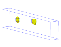
a) $\varepsilon\approx 15$	b) $\mu\approx 2$

Figure 9: Computed images of reconstructed functions $\varepsilon(x)$ and $\mu(x)$ from backscattering data with 3% additive noise, frequency $\omega=21$.

Figure 10: Zoomed reconstructions of $\varepsilon$ (top row) and $\mu$ (bottom row). Frequency $\omega=21$ additive noise 3%.

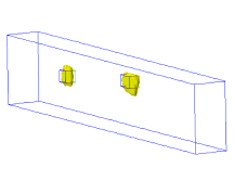
a) $\varepsilon\approx 15$	b) $\mu\approx 2$

Figure 11: Computed images of reconstructed functions $\varepsilon(x)$ and $\mu(x)$ from backscattering data with 10% additive noise, frequency $\omega=21$.

Figure 12: Zoomed reconstructions of $\varepsilon$ (top row) and $\mu$ (bottom row). Frequency $\omega=21$ additive noise 10%.

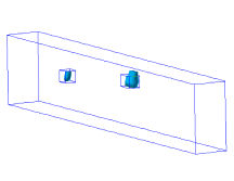
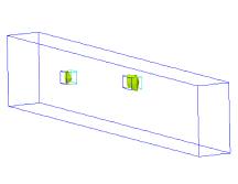
a) $\varepsilon\approx 11.3$	b) $\mu\approx 1.7$

Figure 13: Computed images of reconstructed functions $\varepsilon(x)$ and $\mu(x)$ from backscattering data with 3% additive noise, frequency $\omega=30$.

Figure 14: Zoomed reconstructions of $\varepsilon$ (top row) and $\mu$ (bottom row). Frequency $\omega=30$ additive noise 3%.

a) $\varepsilon\approx 11.2$	b) $\mu\approx 1.7$

Figure 15: Computed images of reconstructed functions $\varepsilon(x)$ and $\mu(x)$ from backscattering data with 10% additive noise, frequency $\omega=30$.

Figure 16: Zoomed reconstructions of $\varepsilon$ (top row) and $\mu$ (bottom row). Frequency $\omega=30$ additive noise 10%.

6 Discussion and Conclusion

In this work we have used time dependent backscattering data to simultaneously reconstruct both coefficients, $\varepsilon(x)$ and $\mu(x)$, in the Maxwell’s system as well as their locations. In order to do that we have used optimization approach which was similar to the method used in [4]. We tested our algorithm with two different noise levels (3% and 10% of additive noise) and with two different frequencies ($\omega=21$ and $\omega=30$, see (27)). The bigger noise level (10%) seemed to produce artefact in reconstructing $\varepsilon$ with frequency $\omega=30$, see figure 15. However, we are able to reconstruct functions $\varepsilon(x)$ and $\mu(x)$ with contrasts that are within the limits of (29). An important observation is that in our computations, we are able to obtain large contrasts for dielectric function $\varepsilon(x)$ which allows us to conclude that we are able to reconstruct metallic targets. At the same time, the contrast for the function $\mu(x)$ is within limits of (29). We could reconstruct size on z-direction for $\varepsilon$, however, size for $\mu(x)$ should be still improved.

In our future research, we are planning to refine the obtained images through the adaptive finite element method in order to get better shapes and sizes of the inclusions. In [7, 4, 6] it was shown that this method is powerful tool for the reconstruction of heterogeneous targets, their locations and shapes accurately.

We note that our algorithm of simultaneous reconstruction of both parameters as well as its adaptive version can also be applied for the case when usual edge elements are used for the numerical simulation of the forward and adjoint problems in step 1 of our algorithm, see [16, 17, 25] for finite element analysis and discretization in this case. This as well as comparison between two different discretization techniques for the solution of our CIP can be considered as a challenge fot the future research.

References

- [1] (MR1253460) F. Assous, P. Degond, E. Heintze and P. Raviart, On a finite-element method for solving the three-dimensional Maxwell equations, Journal of Computational Physics, 109 (1993), 222–237.
- [2] (MR2757493) A. Bakushinsky, M. Y. Kokurin, A. Smirnova, Iterative Methods for Ill-posed Problems, Inverse and Ill-Posed Problems Series 54, De Gruyter, 2011.
- [3] (MR3015394) L. Beilina, Energy estimates and numerical verification of the stabilized Domain Decomposition Finite Element/Finite Difference approach for time-dependent Maxwell’s system, Central European Journal of Mathematics, 11 (2013), 702-733 DOI: 10.2478/s11533-013-0202-3.
- [4] L. Beilina, Adaptive Finite Element Method for a coefficient inverse problem for the Maxwell’s system, Applicable Analysis, 90 (2011) 1461-1479.
- [5] L. Beilina, M. Grote, Adaptive Hybrid Finite Element/Difference Method for Maxwell’s equations, TWMS Journal of Pure and Applied Mathematics, V.1(2), pp.176-197, 2010.
- [6] (MR2110450) L. Beilina and C. Johnson, A posteriori error estimation in computational inverse scattering, Mathematical Models in Applied Sciences, 1 (2005), 23-35.
- [7] L. Beilina, N. T. Thành, M. V. Klibanov, J. Bondestam-Malmberg, Reconstruction of shapes and refractive indices from blind backscattering experimental data using the adaptivity, Inverse Problems, 30 (2014), 105007
- [8] (MR3162104) L. Beilina, N. T. Thành, M. V. Klibanov, M. A. Fiddy, Reconstruction from blind experimental data for an inverse problem for a hyperbolic equation, Inverse Problems, 30 (2014), 025002.
- [9] M.I. Belishev and V.M. Isakov On the Uniqueness of the Recovery of Parameters of the Maxwell System from Dynamical Boundary Data, Journal of Mathematical Sciences 122 (2004), 3459-3469.
- [10] (MR2966179) M. Bellassoued, M. Cristofol, and E. Soccorsi Inverse boundary value problem for the dynamical heterogeneous Maxwell’s system, Inverse Problems, 28 (2012), 095009.
- [11] S. C. Brenner and L. R. Scott, The Mathematical theory of finite element methods Springer-Verlag, Berlin, 1994.
- [12] (MR2719775) P. Caro Stable determination of the electromagnetic coefficients by boundary measurements, Inverse Problems, 26 (2010), 105014.
- [13] (MR2581979) P. Caro, P. Ola and M. Salo Inverse boundary value problem for Maxwell equations with local data, Communications in Partial Differential Equations, 34 (2009), 1425-1464.
- [14] J. M. Catalá-Civera, A.J. Canós-Marin, L. Sempere and E. de los Reyes Microwaveresonator for the non-invasive evaluation of degradation processes in liquid composites, IEEE Electronic Letters, 37 (2001), 99-100.
- [15] H. S. Cho, S. Kim, J. Kim and J. Jung, Determination of allowable defect size in multimode polymer waveguides fabricated by printed circuit board compatible processes, Journal of Micromechanics and Microengineering, 20 (2010), doi:10.1088/0960-1317/20/3/035035.
- [16] P. Ciarlet, Jr. and J. Zou, Fully discrete finite element approaches for time-dependent Maxwell’s equations, Numerische Mathematik 82 (1999), 193-219.
- [17] (MR3188392) P. Ciarlet, Jr., H. Wu and J. Zou, Edge element methods for Maxwell’s equations with strong convergence for Gauss’ laws, SIAM Journal on Numerical Analysis 52 (2014), 779-807.
- [18] G. C. Cohen, Higher order numerical methods for transient wave equations, Springer-Verlag, 2002.
- [19] R. Courant, K. Friedrichs and H. Lewy On the partial differential equations of mathematical physics, IBM Journal of Research and Development, 11 (1967), 215-234.
- [20] D. W. Einters, J. D. Shea, P. Komas, B. D. Van Veen and S. C. Hagness Three-dimensional microwave breast imaging: Dispersive dielectric properties estimation using patient-specific basis functions IEEE Transactions on Medical Imaging 28 (2009), 969–981
- [21] M. Eller, V. Isakov, G. Nakamura and D.Tataru Uniqueness and stability in the Cauchy problem for Maxwell and elasticity systems, in Nonlinear Partial Differential Equations and their Applications, Collège de France Seminar, 14 (2002), 329-349.
- [22] A. Elmkies and P. Joly, Finite elements and mass lumping for Maxwell’s equations: the 2D case. Numerical Analysis, 324 (1997), 1287–1293.
- [23] (MR0436612) H. W. Engl, M. Hanke and A. Neubauer, Regularization of Inverse Problems Boston: Kluwer Academic Publishers, 2000.
- [24] B. Engquist and A. Majda, Absorbing boundary conditions for the numerical simulation of waves, Mathematics of Computation, 31 (1977), 629-651.
- [25] (MR2671794) H. Feng, D. Jiang and J. Zou, Simultaneous identification of electric permittivity and magnetic permeability, Inverse Problems, 26 (2010), 095009.
- [26] (MR2324465) M. J. Grote, A. Schneebeli, D. Schötzau, Interior penalty discontinuous Galerkin method for Maxwell’s equations: Energy norm error estimates, Journal of Computational and Applied Mathematics, 204 (2007), 375-386.
- [27] M V de Hoop, L Qiu, and O Scherzer. Local analysis of inverse problems: Höder stability and iterative reconstruction, Inverse Problems, 28 (2012), 045001.
- [28] (MR2804535) K Ito, B Jin, and T Takeuchi Multi-parameter Tikhonov regularization, Methods and Applications of Analysis, 18 (2011), 31–46.
- [29] (MR2032871) P. Joly, Variational methods for time-dependent wave propagation problems, Lecture Notes in Computational Science and Engineering, Springer, 2003.
- [30] M.V. Klibanov, Uniqueness of the solution of two inverse problems for a Maxwellian system, Computational Mathematics and Mathematical Physics, 26 (1986), 67-73.
- [31] Y. Kurylev, M. Lassas and E. Somersalo Maxwell’s equations with a polarization independent wave velocity: Direct and inverse problems, Journal de Mathematiques Pures et Appliquees, 86 (2006), 237-270.
- [32] A.V. Kuzhuget, L. Beilina, M.V. Klibanov, A. Sullivan, L. Nguyen and M.A. Fiddy, Blind experimental data collected in the field and an approximately globally convergent inverse algorithm, Inverse Problems, 28 (2012), 095007.
- [33] (MR1059373) R. L. Lee and N. K. Madsen, A mixed finite element formulation for Maxwell’s equations in the time domain, Journal of Computational Physics, 88 (1990), 284-304.
- [34] (MR2192286) S. Li An inverse problem for Maxwell’s equations in bi-isotropic media SIAM Journal on Mathematical Analysis, 37 (2005), 1027–1043.
- [35] S. Li and M. Yamomoto Carleman estimate for Maxwell’s Equations in anisotropic media and the observability inequality, Journal of Physics: Conference Series, 12 (2005) 110-115.
- [36] (MR2177854) S. Li and M. Yamamoto An inverse source problem for Maxwell’s equations in anisotropic media, Applicable Analysis, 84 (2005).
- [37] P. B. Monk, Finite Element methods for Maxwell’s equations, Oxford University Press, 2003.
- [38] J. Monzó, A. Díaz, J.V. Balbastre, D. Sánchez-Hernández and E. de los Reyes Selective heating and moisture leveling in microwave-assisted trying of laminal materials:explicit model, 8th Int. Conf. on Microwave and High Frequency heating AMPERE, Bayreuth, Germany, 2001.
- [39] (MR1764247) C. D. Munz, P. Omnes, R. Schneider, E. Sonnendrucker and U. Voss, Divergence correction techniques for Maxwell Solvers based on a hyperbolic model, Journal of Computational Physics, 161 (2000), 484–511.
- [40] (MR0864305) J.C. Nédélec, A new family of mixed finite elements in , NUMMA, 50 (1986), 57-81.
- [41] (MR1224101) P. Ola, L. Päivarinta and E. Somersalo An inverse boundary value problem in electrodynamics, Duke Mathematical Journal, 70 (1993), 617-653.
- [42] K. D. Paulsen and D. R. Lynch, Elimination of vector parasities in Finite Element Maxwell solutions, IEEE Transactions on Microwave Theory and Techniques, 39 (1991), 395-404.
- [43] PETSc, Portable, Extensible Toolkit for Scientific Computation, http://www.mcs.anl.gov/petsc/.
- [44] (MR0725856) O. Pironneau, Optimal shape design for elliptic systems, Springer-Verlag, Berlin, 1984.
- [45] J. Pitarch, M. Contelles-Cervera, F. L Pe aranda-Foix, J. M. Catal -Civera, Determination of the permittivity and permeability for waveguides partially loaded with isotropic samples, Measurement Science and Technology, 17 (2006), 145-152.
- [46] (MR2783934) M. Salo, C. Kenig and G. Uhlmann Inverse problems for the anisotropic Maxwell equations, Duke Matematical Journal, 157 (2011), 369-419.
- [47] Y. G. Smirnov, Y. G Shestopalov, E. D. Derevyanchyk, Reconstruction of permittivity and permeability tensors of anisotropic materials in a rectangular waveguides from the reflection and transmission coefficients from different frequencies, Proceedings of Progress in Electromagnetic Research Symposium, Stockholm, Sweden, (2013), 290-295.
- [48] D. R. Smith, S. Schultz, P. Markos and C. M. Soukoulis, Determination of effective permittivity and permeability of metamaterials from reflection and transmission coefficients, Physical Review B, 65 (2002), DOI:10.1103/PhysRevB.65.195104.
- [49] N. T. Thành, L. Beilina, M. V. Klibanov, M. A. Fiddy, Reconstruction of refractive indices from experimental back-scattering data using a globally convergent method, SIAM J. Scientific Computing,36 (3) (2014), 273-293.
- [50] A. N. Tikhonov, A. V. Goncharsky, V. V. Stepanov and A. G. Yagola, Numerical Methods for the Solution of Ill-Posed Problems Kluwer, London, 1995.
- [51] WavES, the software package, http://www.waves24.com.
- [52] X. Zhang, H. Tortel, S. Ruy and A. Litman Microwave imaging of soil water diffusion using the linear sampling method, IEEE Geoscience and Remote Sensing Letters 8 (2011),421–425