A Bayesian estimate of the CMB-large-scale structure cross-correlation

Abstract

Evidences for late-time acceleration of the Universe are provided by multiple probes, such as Type Ia supernovae, the cosmic microwave background (CMB) and large-scale structure (LSS). In this work, we focus on the integrated Sachs–Wolfe (ISW) effect, i.e., secondary CMB fluctuations generated by evolving gravitational potentials due to the transition between, e.g., the matter and dark energy (DE) dominated phases. Therefore, assuming a flat universe, DE properties can be inferred from ISW detections. We present a Bayesian approach to compute the CMB–LSS cross-correlation signal. The method is based on the estimate of the likelihood for measuring a combined set consisting of a CMB temperature and a galaxy contrast maps, provided that we have some information on the statistical properties of the fluctuations affecting these maps. The likelihood is estimated by a sampling algorithm, therefore avoiding the computationally demanding techniques of direct evaluation in either pixel or harmonic space. As local tracers of the matter distribution at large scales, we used the Two Micron All Sky Survey (2MASS) galaxy catalog and, for the CMB temperature fluctuations, the ninth-year data release of the Wilkinson Microwave Anisotropy Probe (WMAP9). The results show a dominance of cosmic variance over the weak recovered signal, due mainly to the shallowness of the catalog used, with systematics associated with the sampling algorithm playing a secondary role as sources of uncertainty. When combined with other complementary probes, the method presented in this paper is expected to be a useful tool to late-time acceleration studies in cosmology.

1. Introduction

Understanding the origin of the late-time acceleration of the Universe has been one of the biggest challenges in cosmology in the past almost 20 yrs. A combined analysis of independent data sets, such as distance measurements of Type Ia supernovae (Betoule et al., 2014), measurements of the cosmic microwave background (CMB) anisotropies (Bennett et al., 2013; Planck Collaboration, 2015a) and observations of the large-scale structure (LSS) in the universe (Alam et al., 2015), indicate that the cosmos has the following energy budget: $\sim 5\%$ of baryonic matter, $\sim 26\%$ of dark matter and $\sim 69\%$ of dark energy (DE). From the theoretical point of view, a variety of DE models have been proposed, involving different DE equations of state (Joyce et al., 2015), canonical and noncanonical scalar fields (Carvalho et al., 2006; Copeland et al., 2006), and $f(R)$ gravity (Nojiri & Odintsov, 2011), among others, to explain the recent cosmic acceleration.

The study of the statistical properties of fluctuations of the different constituents of the Universe is a powerful method to select among the various competing cosmological models. For example, useful probes for the late-time cosmic acceleration are the measurements of the cross-correlation between the CMB temperature fluctuations and LSS tracers. The CMB–LSS cross-correlation has been the subject of a number of papers since Crittenden & Turok (1996) proposed to use the method to detect the integrated Sachs–Wolfe (ISW) effect independently of the intrinsic CMB fluctuations. In the case where the gravitational potentials decay, a positive correlation is expected (Cooray, 2002), meaning that at large scales, hot spots in the CMB will correspond to overdense regions in the galaxy distribution. This positive correlation is also expected in open universes (Kamionkowski, 1996; Kinkhabwala & Kamionkowski, 1999), whereas a negative correlation will occur in closed ones.

Several authors reported detections (sometimes in contradiction; see Dupé et al. (2011)) of the ISW effect by computing the cross-correlation between the first-year Wilkinson Microwave Anisotropy Probe (WMAP) data with radio sources (Boughn & Crittenden, 2002; Nolta et al., 2004; Boughn & Crittenden, 2005a, b); the hard X-ray background (Boughn & Crittenden, 2004a, b); the Sloan Digital Sky Survey (SDSS) Data Realease 1 (Fosalba et al., 2003; Padmanabhan et al., 2005; Abazajian et al., 2009), the Two Micron All Sky Survey (2MASS; Afshordi et al. (2004)), the APM Galaxy Survey (Fosalba & Gaztanaga, 2004; Hernández-Monteagudo et al., 2014), and a combination of the above (Gaztanaga et al., 2006). The third-year WMAP data were correlated by Cabre et al. (2006) with the fourth SDSS data release (DR4), showing a significant positive signal, while Giannantonio et al. (2006) compared it with high-redshift SDSS quasars, claiming a $2\sigma$ detection (see also Ho et al. (2008)). McEwen et al. (2007) used a directional spherical wavelet analysis and found a positive detection at the $3.9\sigma$ level. ISW detections about $3\sigma$ were also obtained using the Wide-field Infrared Survey Explorer (WISE) and seventh-year (Goto et al., 2012) and ninth-year WMAP data (Ferraro et al., 2015).

More recently, the Planck satellite has released the results of its full data set, including the claim of an ISW effect detection at the $2\sigma-4\sigma$ level (Planck Collaboration (2014, 2015c); see also Granett et al. (2015)). They observed an exceeding amplitude of the ISW signal measured with superclusters and voids. Such result confirms previous measurements by, e.g., Granett et al. (2008) and Nadathur et al. (2012), also using localized measurements of superstructures, and Giannantonio et al. (2012), cross-correlating WMAP CMB maps and SDSS observations, who found an ISW signal indicating a discrepancy with respect to what is expected by the $\Lambda\text{CDM}$ model. In an attempt to find possible reasons for this tension, authors have dedicated efforts in better understanding the systematics and checking for possible contamination signals, e.g. point sources and Galactic foreground, besides using the recently released Planck products, namely, CMB lensing potential maps and polarization data (Goto et al., 2012; Nadathur et al., 2012; Ferraro et al., 2015; Planck Collaboration, 2015c).

Given the number of different data sets used, especially the ones taken as LSS tracers, and the several methods employed, points such as (i) the statistical significance of the signal and (ii) the systematics affecting both the data sets used, as well as (iii) the procedure adopted, become particularly important in order to properly interpret the results (see Giannantonio et al. (2012) and references therein). In this work we address some of these questions by using Bayesian inference to study in detail the correlation between the WMAP9 temperature maps (Bennett et al., 2013) and the catalog of luminous sources of the 2MASS infrared survey (Skrutskie et al., 2006).

Bayesian inference applied to CMB data has become very popular in the past two decades, particularly in situations in which the computation of a likelihood matrix is required. The particular case of obtaining the maximum likelihood estimate for the CMB autocorrelation power spectrum, provided that some properties of the noise and of the foregrounds are known, is an example where Bayesian inference has shown its full power (see, e.g., Bond (1998)). However, the direct evaluation of this likelihood for satellites with fine angular resolution, such as WMAP and Planck, has also been revealed to be a hard computational problem, with a number of operations scaling beyond the current capacity of computers (Hivon et al., 2002). To overcome this technical problem, cosmologists have developed techniques based on Markov chain algorithms in order to reconstruct the likelihood for CMB measurements. Gibbs sampling is one of these Monte Carlo (MC) based techniques and has been successfully used to estimate the CMB (temperature and polarization) power spectra (Jewell et al., 2004; Wandelt et al., 2004; Eriksen et al., 2004; Larson et al., 2007; Dunkley et al., 2009). Here we apply the Gibbs sampling method to a combined CMB-galaxy survey experiment whose measurements, as in the CMB-only case, contain the primordial signal of interest, instrumental noise and, in principle, residual foregrounds. Once some assumptions on the statistical properties of the noise were made, we extracted a Bayesian estimate for the primordial signal full covariance matrix, containing the autocorrelation power spectra of the CMB and of the galaxies in its diagonal and, most important in this work, the cross-correlation power spectrum as off-diagonal elements. Here we focus on determining the potential of a galaxy catalog with the widest possible sky coverage, such as 2MASS, to show a cross-correlation signal at large angular scales with a CMB temperature map. A study on the strength of such a signal, using deeper surveys (at the cost of sky coverage), is left for a future work.

The paper is organized as follows. In Section 2 we outline the theoretical background in order to calculate the expected cross-correlation spectrum between the CMB and an LSS tracer when the ISW effect is present. The effect of a cut-sky map on the estimates of cross-correlation power spectrum is discussed in Section 3 and the usual mask deconvolution algorithm to retrieve the ensemble average estimate for this spectrum is also discussed. Section 4 is devoted to the detailed presentation of the Gibbs sampling method applied here to a combined CMB–galaxy survey data set, the validation of which is presented in Section 6. The application of the analysis pipeline, described in section 5, to the WMAP9–2MASS combined data set is found in Section 7. Final remarks are then presented in Section 8.

2. The CMB–LSS cross-correlation

In this section we briefly present the theoretical background to compute the ISW and LSS auto- and cross-correlation functions. The ISW effect is a secondary anisotropy in the CMB temperature field due to a variation of the gravitational potential along the line of sight in a direction $\hat{\mathbf{n}}$, i.e.,

$$\Delta_{t}^{\text{ISW}}(\hat{\mathbf{n}})\equiv\left(\frac{\Delta T(\hat{\mathbf{n}})}{T}\right)=-2\int dz\,e^{-\tau(z)}~{}{d\Phi\over{dz}}(\hat{\mathbf{n}},z),$$ (1)

where $\tau$ is the optical depth of CMB photons and $\Phi(\hat{\mathbf{n}},z)$ is the Newtonian gravitational potential at redshift $z$. Using the Poisson equation in the Fourier space, $\Phi(\mathbf{k},z)$ is given by

$$\Phi(\mathbf{k},z)=\frac{3}{2}\Omega_{m}\left(\frac{H_{0}}{c\,k}\right)^{2}(1+z)\delta(\mathbf{k},z),$$ (2)

where $\Omega_{m}$ is the dimensionless matter density today, $c$ is the speed of light, $H_{0}$ is the Hubble parameter, and $\delta(\mathbf{k},z)$ is the density contrast of matter.

Similarly, the galaxy fluctuations can be written as

$$\Delta_{g}(\hat{\mathbf{n}})\equiv\left(\frac{n_{g}(\hat{\mathbf{n}})-\bar{n}_{g}}{\bar{n}_{g}}\right)=\int dz\,b_{g}(z)\frac{dN}{dz}(z)\delta(\mathbf{k},z),$$ (3)

where $\bar{n}_{g}$ is the mean number density of galaxies, $b_{g}(z)$ is the linear bias factor [$\delta_{g}(z)=b_{g}(z)\delta(z)$] and $dN/dz$ is the normalized galaxy redshift distribution (Afshordi et al., 2004; Rassat et al., 2007; Giannantonio et al., 2014).

From Equations (1) – (3), the two-point correlation function $\langle\Delta_{x}(\hat{\mathbf{n}})\Delta_{y}(\hat{\mathbf{n}}^{\prime})\rangle$ in harmonic space is

$$C_{l}^{xy}=\frac{2}{\pi}\int dk\,k^{2}W_{l}^{x}(k)W_{l}^{y}(k)P(k),$$ (4)

where $x,y=(t,g)$, and $P(k)$ is the matter power spectrum. The ISW and galaxy autocorrelation functions, $C_{l}^{tt}$ and $C_{l}^{gg}$, as well as the CMB(ISW)–galaxy cross-correlation $C_{l}^{tg}$ are computed substituting into Equation (4) the respective kernels, namely,

$$W^{t}(k,z) = -3\Omega_{m}\left(\frac{H_{0}}{k\,c}\right)^{2}\int dz\,\frac{d\left[(1+z)D(z)\right]}{dz}\,j_{l}[k\chi(z)],$$

$$W^{g}(k,z) = \int dz\,b_{g}(z)\frac{dN}{dz}D(z)j_{l}[k\chi(z)],$$ (5)

where $D(z)$ is the linear growth function (normalized to one at $z=0$), $j_{l}[k\chi(z)]$ is the spherical Bessel function of the first kind, and $\chi(z)$ is the comoving distance.

3. Cross-correlation with partial sky coverage

Partial and/or nonuniform sky coverage is a typical situation for CMB and galaxy survey experiments due to a limited field of view, galactic foregrounds, dust extinction, etc. For a CMB experiment, the strong galactic emission at radio and microwave wavelengths, for example, forces the masking of large regions of the sky maps close to the galactic plane, in order to get a reliable estimate of the CMB temperature power spectrum. At small angular scales, the positions of identified extragalactic sources also have to be removed. The same galactic emissions affect the detection of galaxies close to the Milky Way plane, and even at high galactic latitudes, dust extinction has to be taken into account when calculating magnitudes.

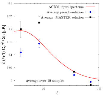
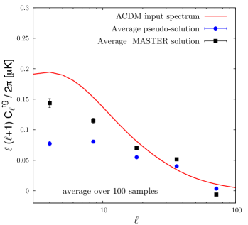
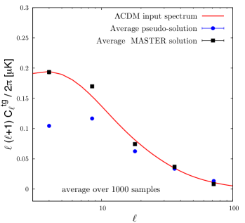
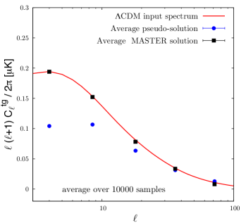
Figure 1.— Convergence of the MASTER binned (a total of six bins approximately logarithmically spaced over $3\leq\ell\leq 192$) solution for the CMB–LSS cross-power spectrum for different numbers of sky realizations. The mask used was WMAP9 KQ85 with $f_{sky}=0.77$; the fiducial cosmological model is $\Lambda$CDM (only linear theory), with parameters given in Table 1 and with a galaxy bias factor $b_{g}=1.4$ and the selection suited for band 4 of the 2MASS catalog. The pseudo-$C_{\ell}$ estimate is also shown, and its power is depleted at all scales, but the damping is particularly strong at large angular scales ($\ell<10$), irrespective of the number of samples. Uncertainties are the errors on the average. For the cosmic variance contribution to $C_{\ell}^{tg}$ see Figures 13 and 15.

When retrieving spherical harmonics coefficients from a cut-sky map, the effect of the mask, taken here as a weight function $W(\hat{\mathbf{n}})$ in the direction of the unit vector $\hat{\mathbf{n}}$, is to mix different multipoles (Hivon et al., 2002), leading to the so-called pseudo-power spectra $\langle\tilde{C}_{\ell}\rangle$. If the mask power spectrum ${\cal W}_{\ell}$, the $\ell$-space window function of the beam $B_{\ell}$, and an estimate of the instrumental noise power $N_{\ell}$ are available, as shown in Hivon et al. (2002), one can retrieve an estimate for the ensemble average of the true power spectrum $\langle C_{\ell}\rangle$, by solving the following linear system:

$$\langle\tilde{C}_{\ell}\rangle=\sum_{\ell^{\prime}}M_{\ell\ell^{\prime}}B_{\ell^{\prime}}^{2}\langle C_{\ell^{\prime}}\rangle+\langle N_{\ell}\rangle,$$ (6)

where $M_{\ell\ell^{\prime}}$ is the multipole mixing matrix that can be written in terms of the Wigner-$3j$ symbols

$$M_{\ell\ell^{\prime}}=\frac{2\ell^{\prime}+1}{4\pi}\sum_{\ell^{\prime\prime}}(2\ell^{\prime\prime}+1){\cal W}_{\ell^{\prime\prime}}\left(\begin{array}[]{ccc}\ell&\ell^{\prime}&\ell^{\prime\prime}\\ 0&0&0\end{array}\right)^{2}.$$ (7)

The mixing pattern is strongly dependent on the shape of the mask, but for the particular case of a constant power spectrum $\langle C_{\ell}\rangle=C=cte$, like in the case of white noise, it leads to a simple power damping at all scales given by the sky fraction $f_{\text{sky}}$ covered by the unmasked directions $\langle\tilde{C}\rangle=Cf_{sky}$ .

Cross-correlation analyses of the CMB and galaxy survey maps have been performed in the literature using pseudo-$C_{\ell}$’s estimators (Rassat et al., 2007; Ho et al., 2008; Xia et al., 2011; Giannantonio et al., 2012). As an ensemble average, the solution of Equation (6) will eventually converge to the true power spectrum in the limit of a large number of sky realizations. Having a single universe to retrieve the sky map multipoles, such an estimator is severely affected by cosmic variance at low multipoles. We have quantified the impact of cosmic variance in the MASTER (Monte Carlo Apodized Spherical Transform Estimator; Hivon et al. (2002)) solution for the CMB–LSS cross-power spectrum using MC simulations and $\Lambda$CDM as the fiducial cosmological model (see Table 1). Figure 1 shows the convergence of a binned MASTER solution toward the true value for different sets of sky realizations. Auto- and cross-correlation power spectra have been generated from the fiducial model with a bias factor $b_{g}=1.4$ and a selection function appropriate for band 4 of the 2MASS catalog (see eq. 20 and section 4 ahead), from which the respective sky maps for the CMB and galaxy survey were synthesized using the HEALPix synfast program . The WMAP9 KQ85 analysis mask was then applied to these maps, and the MASTER solution was retrieved. No instrumental noise has been added to the maps, since for the particular case of cross-correlation between maps measured independently, the average noise cross-power spectrum appearing in Equation (6) is zero. As one can see, the solution will be a reasonable approximation to the true underlying power spectrum for about 1000 sky samples. A single sky-based estimate can be very far from the true value. One can also see the effect of power depletion at large scales due to the masked region, which for the KQ85 mask is about 50% for the quadrupole and octopole.

Table 1Fiducial Cosmological Model: $\Lambda$CDM, flat Universe

Parameter	Symbol	Value
Baryon density	$\Omega_{b}h^{2}$	0.0226
Cold dark matter density	$\Omega_{c}h^{2}$	0.112
Curvature perturbation ($k_{0}=0.002$ Mpc-1)	$\Delta_{\cal R}^{2}$	$2.4\times 10^{-9}$
Scalar spectral index	$n_{s}$	0.96
Reionization optical depth	$\tau$	0.09
Hubble constant (100 km s-1Mpc-1)	$h$	0.7

4. Gibbs sampling approach

Bayesian estimates of the CMB temperature and polarization power spectra have been successfully used by several experiments in recent years. The fluctuations observed today in the photon field temperature distribution over the sky are assumed to come from three main sources: primordial fluctuations generated in the early universe, instrumental noise, and foregrounds. The likelihood for observing a given temperature angular distribution can be calculated once the galactic emission and extragalactic point sources have been removed from the sky maps, and also if appropriate assumptions are made on the statistical properties of the primordial signal and the instrumental noise (Bond, 1998). If performed in pixel space, these calculations were shown to scale as $\mathcal{O}(N_{p}^{3})$, where $N_{p}$ is the total number of pixels, becoming prohibitively expensive in terms of computing power for satellite experiments like WMAP ($N_{p}\sim 10^{6}$) and Planck ($N_{p}\sim 10^{7}$) (Hivon et al., 2002). In order to avoid such brute-force approach of direct evaluation of the likelihood, MC techniques have been implemented in which sample maps of the primordial signal are drawn from the a posteriori probability distribution taking into account cosmic variance, instrumental noise, and residual foregrounds (Eriksen et al., 2004; Jewell et al., 2004; Wandelt et al., 2004; Dunkley et al., 2009). The method can be applied to either Time Order Data (TOD) or pixelized maps and can take into account filtering and beaming effects.

Let $\mathbf{d}$ be a pixelized temperature map consisting of primordial signal $\mathbf{s}$ and instrumental noise $\mathbf{n}$. Assuming that both $\mathbf{s}$ and $\mathbf{n}$ follow Gaussian distributions with covariance matrices $\mathbf{S}$ and $\mathbf{N}$, respectively, the likelihood for observing such a map, after marginalizing over the unknown true signal $\mathbf{s}$, is given by

$$\mathscr{L}=P(\mathbf{d}|\mathbf{C})=\frac{1}{(2\pi)^{n_{\textrm{dim}}/2}|\mathbf{C}|^{1/2}}\textrm{exp}\left(-\frac{1}{2}\mathbf{d}^{\textrm{T}}\mathbf{C}^{-1}\mathbf{d}\right),$$ (8)

where $n_{\textrm{dim}}=N_{p}^{2}$ and $\mathbf{C}$ represents the full covariance matrix ($\mathbf{C}=\mathbf{S}+\mathbf{N}$). The difficulties arising from a direct evaluation of the Equation (8) become evident, since it requires the calculation of the determinant of $\mathbf{C}$ and, in a typical CMB experiment, $\mathbf{S}$ is diagonal in harmonic space, whereas $\mathbf{N}$ is usually close to diagonal in pixel space.

Using the Bayes theorem, we write the likelihood as $P(\mathbf{C}|\mathbf{d})\propto\pi(\mathbf{S})P(\mathbf{d}|\mathbf{C})$, where $P(\mathbf{C}|\mathbf{d})$ is the a posteriori probability density and $\pi(\mathbf{S})$ is the prior on the power spectrum. In Jewell et al. (2004) and Wandelt et al. (2004), an MC method was devised in which $P(\mathbf{C}|\mathbf{d})$ is estimated by building a Markov chain whose stationary state is the joint probability distribution $P(\mathbf{C,s,d})=\pi(\mathbf{S})P(\mathbf{d}|\mathbf{s})P(\mathbf{s}|\mathbf{C})$, and assuming that $\pi(\mathbf{S})=const$. In such a state, samples drawn along the chain can be used to recover $\mathscr{L}$ by marginalizing over the unknown true temperature signal $\mathbf{s}$ with a Blackwell–Rao estimator (Chu et al., 2005; Dunkley et al., 2009). The transition probabilities between two chain states are taken to be the conditional probabilities $P(\mathbf{s}|\mathbf{C,d})$ and $P(\mathbf{C}|\mathbf{s,d})$. Thus, at a certain state in the chain, the current value of $\mathbf{S}$ and the measured sky temperature map $\mathbf{d}$ are used to extract a new signal map $\mathbf{s}$, leading to a new signal covariance matrix $\mathbf{S}$. The method has been successfully applied to MC simulations using high-resolution sky maps in Eriksen et al. (2004), where procedures to deal with the effects of foregrounds and to properly treat the presence of noncosmological monopoles and dipoles have also been presented. Later, the method was naturally extended beyond the $tt$ covariance matrix estimation, allowing for polarization measurements to be included in the vector $\mathbf{d}$ (Larson et al., 2007). Recently this approach was applied to characterize localized secondary anisotropies (Bull et al., 2015).

In this paper, we apply the extended Gibbs sampling method of Larson et al. (2007) to a combined CMB–galaxy survey experiment whose measurements can be represented by a vector $\mathbf{d}$ which, in our case, is the image of a mapping from the 2-sphere $S^{2}$ into $\mathbb{R}^{2}$:

$$f: S^{2} \longrightarrow\mathbb{R}^{2}$$

$$(\theta,\phi) \mapsto(\Delta_{t},\Delta_{g}).$$

As in the CMB case, these measurements contain the primordial signal, instrumental noise, and, in principle, irreducible foregrounds. The signal is also subject to the effect of the experiment beam, represented here by a matrix $\mathbf{B}$. Neglecting the foregrounds for a while, one can write $\mathbf{d}=\mathbf{Bs+n}$ . We are interested in extracting from $\mathbf{d}$ a Bayesian estimate of the primordial signal covariance matrix $\mathbf{S}$, provided that the full noise covariance matrix $\mathbf{N}$ is known. In harmonic space, we can write $\mathbf{s}$ as

$$\mathbf{s}^{\textrm{T}}=(\mathbf{s}^{tg}_{00},\mathbf{s}^{tg}_{10},\mathbf{s}^{tg}_{11},\cdots,\mathbf{s}^{tg}_{\ell_{max}0}\cdots,\mathbf{s}^{tg}_{\ell_{max}\ell_{max}})$$ (9)

and matrix $\mathbf{S}$ as

$$\mathbf{S}=\textrm{diag}(\mathbf{S}_{0}^{tg},\mathbf{S}_{1}^{tg},\mathbf{S}_{1}^{tg},\cdots,\mathbf{S}_{\ell_{max}}^{tg},\cdots,\mathbf{S}_{\ell_{max}}^{tg})$$ (10)

with repeated elements along its diagonal associated with $m=0,\cdots,\ell$. We will assume that the noise covariance is diagonal in pixel space, that is, $\mathbf{N}=\textrm{diag}(\mathbf{N}_{11}^{tg},\cdots,\mathbf{N}_{ii}^{tg},\cdots,\mathbf{N}_{pp}^{tg})$, with

$$\mathbf{s}^{tg}_{\ell m}=\left(\begin{array}[]{c}a_{\ell m}^{t}\\ a_{\ell m}^{g}\end{array}\right),$$ (11)

and

$$\mathbf{S}^{tg}_{\ell}=\left(\begin{array}[]{cc}C_{\ell}^{tt}&C_{\ell}^{tg}\\ C_{\ell}^{tg}&C_{\ell}^{gg}\end{array}\right),\quad\mathbf{N}^{tg}_{ii}=\left(\begin{array}[]{cc}N_{ii}^{tt}&0\\ 0&N_{ii}^{gg}\end{array}\right),$$ (12)

since the noises affecting $\Delta_{t}$ and $\Delta_{g}$ are uncorrelated. One also sees that $\mathbf{S}$ is in fact block-diagonal.

In order to draw samples from the joint probability distribution $P(\mathbf{C,s,d})$, we have to set up all the Markov chain machinery described in Jewell et al. (2004); Wandelt et al. (2004); Eriksen et al. (2004); Larson et al. (2007), and Dunkley et al. (2009). In particular, the conditional probability $P(\mathbf{S}|\mathbf{s,d})=P(\mathbf{S}|\mathbf{s})$ was shown in Larson et al. (2007) to be proportional to an inverse-Wishart distribution (Gupta & Nagar, 1999):

$$P(\mathbf{S}|\mathbf{s})\propto\pi(\mathbf{S})\prod_{\ell}\frac{1}{\sqrt{|\mathbf{S}_{\ell}|^{2\ell+1}}}\textrm{exp}\left[-\frac{1}{2}\textrm{Tr}\left(\bm{\sigma}_{\ell}\mathbf{S}_{\ell}^{-1}\right)\right],$$ (13)

where $\bm{\sigma}_{\ell}$ is a $2\times 2$ matrix containing the total primordial signal power at scale $\ell$,

$$\bm{\sigma}_{\ell}=\sum_{m=-\ell}^{\ell}\mathbf{s}_{\ell m}^{tg}\mathbf{s}_{\ell m}^{tg\dagger}.$$ (14)

The signal map samples are drawn according to $P(\mathbf{s}|\mathbf{S,d})$, which is the a posteriori probability density of the Wiener-filtered data, given the power spectrum of the primordial signal and the observed data. This posterior is a multivariate Gaussian with mean $\bm{\mu}=\mathbf{SB}^{\textrm{T}}(\mathbf{N}+\mathbf{BSB}^{\textrm{T}})^{-1}\mathbf{d}$ and covariance $\mathbf{C}=(\mathbf{S}^{-1}+\mathbf{B}^{\textrm{T}}\mathbf{N}^{-1}\mathbf{B})^{-1}$ (Hobson, 2010).

To produce these samples, we have used the transformed white-noise sampling technique, where a linear transformation is applied over initially independent Gaussian random variables in order to induce the appropriate covariance among them. In Eriksen et al. (2004), it was shown that an elegant way to do that is to write the primordial signal as a sum of a Wiener-filtered map $\boldsymbol{x}$ and a fluctuation field $\boldsymbol{y}$, i.e., $\mathbf{s}=\boldsymbol{x+y}$. If $\bm{\chi}$ and $\bm{\xi}$ are Gaussian random variables with zero mean and unit variance, then $\boldsymbol{x}$ and $\boldsymbol{y}$ can be obtained by solving the following $n_{dim}=(2\times(\ell_{max}+1)^{2})^{2}$-dimensional linear systems:

$$\left[\mathbf{1+S^{\textrm{\tiny{1/2}}}B}^{\textrm{\tiny{T}}}\mathbf{N^{\textrm{\tiny{-1}}}BS^{\textrm{\tiny{1/2}}}}\right]\mathbf{S^{\textrm{\tiny{-1/2}}}}\boldsymbol{x} = \mathbf{S^{\textrm{\tiny{1/2}}}B}^{\textrm{{\tiny{T}}}}\mathbf{N^{\textrm{\tiny{-1}}}d},$$ (15)

$$\left[\mathbf{1+S^{\textrm{\tiny{1/2}}}B}^{\textrm{\tiny{T}}}\mathbf{N^{\textrm{\tiny{-1}}}BS^{\textrm{\tiny{1/2}}}}\right]\mathbf{S^{\textrm{\tiny{-1/2}}}}\boldsymbol{y} = \bm{\xi}+\mathbf{S^{\textrm{\tiny{1/2}}}B^{\textrm{\tiny{T}}}N^{\textrm{\tiny{-1/2}}}}\bm{\chi}.$$ (16)

To speed up the process, this system is solved iteratively by using a Conjugate Gradient (CG) method, provided that a good preconditioner matrix is chosen that approximates the inverse of the matrix $\mathbf{1+S^{1/2}B^{T}N^{-1}BS^{1/2}}$ appearing on the left-hand side of Equation (16). Here we have used a block-diagonal preconditioner $\mathbf{M}=\textrm{diag}(\mathbf{M}_{00},...,\mathbf{M}_{\ell m},...,\mathbf{M}_{\ell_{max}\ell_{max}})$, whose elements in harmonic space are simply

$$\mathbf{M}_{\ell m}=\left[\mathbf{1}+\mathbf{S}_{\ell}^{1/2}\mathbf{B}^{T}_{\ell}\mathbf{N}^{-1}_{\ell m}\mathbf{B}_{\ell}\mathbf{S}^{1/2}\right]^{-1},$$ (17)

with the harmonic space beam matrix given by $\mathbf{B}_{\ell}=\textrm{diag}(B_{\ell}^{t},B_{\ell}^{g})$. The inverse noise covariance matrix $\mathbf{N}^{-1}_{\ell m}=\textrm{diag}(1/N^{tt}_{\ell m},1/N^{gg}_{\ell m})$ is obtained by decomposing the corresponding pixel-space inverse noise RMS maps into spherical harmonics $N^{-1}(\theta,\phi)=\sum_{\ell m}a_{\ell m}^{(n)}Y_{\ell m}(\theta,\phi)$. In the case of partial and/or nonuniform sky coverage, $N^{-1}(\theta,\phi)$ is set to zero at unobserved pixels and proportional to the number of observations in all the other pixels. This, in turn, provides an elegant way to deal with foregrounds, where the statistical significance of contaminated pixels can be set to zero by taking $N^{-1}(\theta,\phi)=0$ for these pixels. This is the so-called COMMANDER method (Eriksen et al., 2004). Thus, one can write (Hivon et al., 2002)

$$N^{-1}_{\ell m}=(-1)^{m}(2\ell+1)\sum_{\ell^{\prime}=0}^{\ell_{max}}a_{\ell^{\prime}0}^{(n)}\left(\frac{2\ell^{\prime}+1}{4\pi}\right)^{1/2}\alpha_{\ell\ell^{\prime}m}$$ (18)

with

$$\alpha_{\ell\ell^{\prime}m}=\left(\begin{array}[]{ccc}\ell&\ell&\ell^{\prime}\\ 0&0&0\end{array}\right)\left(\begin{array}[]{ccc}\ell&\ell&\ell^{\prime}\\ m&-m&0\end{array}\right).$$ (19)

5. Data sets, Processing, and analysis pipeline

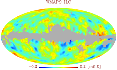
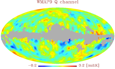
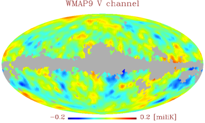
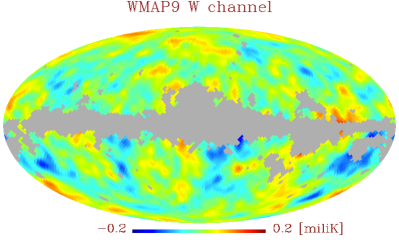
Figure 2.— Mollweide projections in galactic coordinates of the four WMAP9 temperature maps (ILC, Q, V and W channels) in HEALPix pixelization ($nside=32$). A Gaussian beam of $4^{\circ}.9$ (see text) has been applied to the ILC map and $5^{\circ}$ to the other three maps, before the primary temperature analysis mask KQ85 was used.

As explained in Section 4, the Bayesian method underlying the Gibbs sampling relies on the fact that the statistical properties of the instrumental noise are known through the covariance matrix ${\bf N}$. Moreover, the conditional probabilities presented there assume that the fluctuations in the signal and in the noise are Gaussian. Finally, to ensure that the algorithm converges, the signal has to be sampled to sufficiently large multipoles, that is, up to regions of low signal-to-noise ratio (S/N).

In this work, we have used the data from WMAP9 Q (40 GHz), V (60 GHz) and W (90 GHz) channels, as well as the Internal Linear Combination (ILC) CMB temperature map (Bennett et al., 2013; Hinshaw et al., 2013), formed from the linear combination of five smoothed intensity maps (taken from the three previous channels) by minimizing the temperature variance. We have verified that the noise power observed in the high-resolution temperature intensity (I) maps of WMAP9 is fairly well modeled by uncorrelated and Gaussian fluctuations with variances given by $\sigma_{0}^{2}/N_{obs}$, and $\sigma_{0}$ for each channel taken from Greason et al. (2012). To avoid sampling the signal at very high multipoles, where the CMB power spectrum can be alternatively estimated by the MASTER algorithm, they have applied an effective $5^{\circ}$ beam to the ILC map, followed by the addition of uncorrelated white noise of appropriate RMS strength ($\sigma_{0}=2\ \mu$K). The noise amplitude is chosen so that (a) it overcomes the correlation introduced in the noise at small scales by the beam; (b) the added noise dominates over the primordial signal for multipoles $\ell\buildrel>\over{\sim}60$, while keeping the likelihood essentially unchanged at large scales; and (c) the statistical properties of the added noise are completely known.

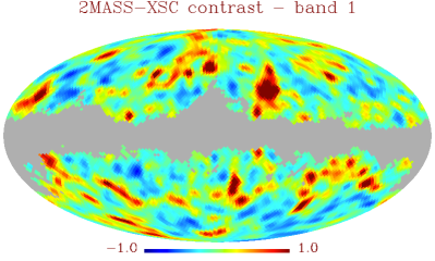
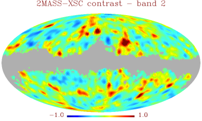
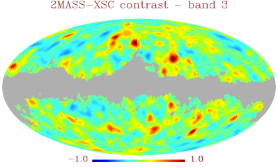
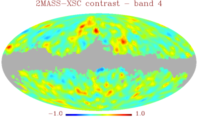
Figure 3.— Mollweide projections in galactic coordinates of the 2MASS–XSC contrast maps in HEALPix pixelization ($nside=32$) for the four corrected $K_{20}$ magnitude bands. A Gaussian beam of $5^{\circ}$ FWHM has been applied. Pixels were masked to avoid the intense emission and dust extinction close to the galactic plane.

The high-resolution maps provided by the LAMBDA website ($nside=512$) were degraded to $nside=32$. The primary temperature analysis mask KQ85 was also degraded using the method described in Bennett et al. (2013), where a pixel at the new resolution is unmasked if at least 50% of the higher-resolution pixels are unmasked. In particular, this corresponds to 9496 out of 12,288 pixels, or 77.3% of the sky. Figure 2 shows the final cut-sky temperature maps, with a $5^{\circ}$ Gaussian beam applied in the case of Q-, V-, and W-band maps (original beams can be neglected) and an additional $4^{\circ}.9$ on the ILC map (since it is already smoothed at $1^{\circ}$), in order to get an effective beam of $5^{\circ}$. The resolution degradation is performed after the beaming.

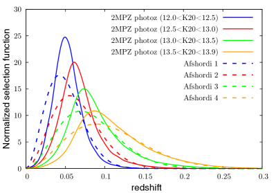
Figure 4.— Normalized selection functions for the 2MASS catalog. The dashed lines show the parameterizations of Afshordi et al. (2004) based on a fit to the $K$-band magnitudes distributions, and the solid lines the photometric redshift distributions of 2MPZ.

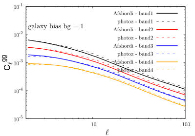
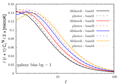
Figure 5.— Expected signals for different 2MASS galaxy selection functions (see eqs. 4 and 5). (a) Galaxy autocorrelation signal. (b) CMB–galaxy cross-correlation signal.

As a tracer of the dark matter distribution at large scales, we have used the XSC (eXtended Source Catalog) of the near-IR 2MASS (Skrutskie et al., 2006). This catalog contains positions, photometry, and basic shape information of 1,647,599 resolved sources, most of which are galaxies ($\sim$ 97%). In order to build the galaxy count map, the following procedure was adopted:

1. The 2MASS $K_{S}$-band (2.16 $\mu$m) 20 mag arcsec^-2 isophotal circular aperture magnitudes (‘k_m_i20c’ called here simply $K_{20}$) were corrected for galactic extinction using the reddening maps $(E(B-V))$ at 100 $\mu$m of Schlegel et al. (1998), according to the expression $K_{20}\rightarrow K_{20}^{\prime}=K_{20}-A_{k}$, where $A_{k}=0.367E(B-V)$.

2. A HEALPix resolution parameter $nside=32$ was adopted, and pixels were masked whenever $A_{k}>0.05$, which leaves 71.6% of the sky with unmasked pixels; only objects with uniform detection were kept (cc_flag != “a” and “z” ) and artifacts have been removed (flag use_src = 1).

3. The final galaxy counting map has 801,476 objects with $12<K^{\prime}_{20}<14$, which were further divided into four magnitude bands. Table 2 summarizes the number of objects in each band, as well as the parameters of the redshift distribution of these sources [see Equation (3)]. Following Afshordi et al. (2004), this distribution can be parameterized by a generalized gamma function, namely,

   $$\frac{dN}{dz}(z|\{\lambda,\beta,z_{0}\})dz=\frac{\beta}{\Gamma(\lambda)}\left(\frac{z}{z_{0}}\right)^{\beta\lambda-1}\exp\left[-\left(\frac{z}{z_{0}}\right)^{\beta}\right]\frac{dz}{z_{0}},$$ (20)

   where $\lambda>0$, $\beta>0$ and $z_{0}>0$. Figure 3 shows the four 2MASS final contrast maps, already masked and smoothed by a $5^{\circ}$ FWHM Gaussian beam. The input map has $nside=64$, and then the beam is applied (excluding masked pixels) and the resolution is degraded to $nside=32$.

Table 2Summary of 2MASS Galaxy Counts in Each of the Four $K_{20}^{\prime}$ Magnitude Bands and the Parameters Describing the Redshift Distribution of These Objects.

Band	$z_{0}$	$\beta$	$\lambda$	$N_{\text{total}}$ (Unmasked)
$12.0<K_{20}^{\prime}<12.5$	0.043	1.825	1.524	51263
$12.5<K_{20}^{\prime}<13.0$	0.054	1.800	1.600	105930
$13.0<K_{20}^{\prime}<13.5$	0.067	1.765	1.636	224345
$13.5<K_{20}^{\prime}<14.0$	0.084	1.723	1.684	469782
Note: Magnitudes were corrected by reddening.

It is worth mentioning that the 2MASS-XSC catalog has been recently improved with the addition of photometric redshifts to a large fraction of its sources (Bilicki et al., 2014). This new sample is called the 2MPZ (2MASS Photometric Redshift) catalog. By cross-correlating XSC with WISE and SuperCOSMOS, the authors were able to obtain photo-$z$’s with errors essentially independent of distance, determined with a spectroscopic redshift subsample, being the median of relative error of about 12%. A hard magnitude cut at $K_{20}^{\prime}<13.9$, the completeness limit of 2MASS, was applied over a slightly different magnitude (calculated using the isophotal elliptical aperture magnitude k_m_k20fe, instead of the circular aperture ‘k_m_i20c’ adopted by us). In terms of galaxy counts, this cut introduces differences that are maximum in band 4, reducing the counts by about 30% with respect to the full XSC. However, we have checked that the galaxy reduction is mostly uniform over the sky and that their partial-sky autocorrelation power spectra, after an $f_{\text{sky}}$ correction and shot-noise subtraction, are completely consistent, within statistical uncertainties, in all four corrected magnitude bands.

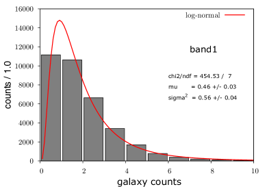
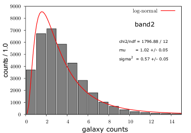
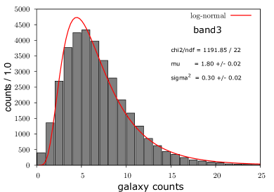
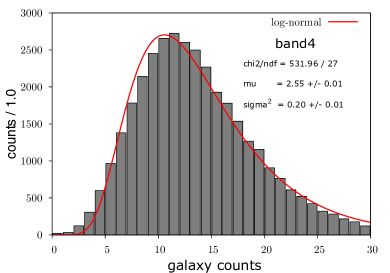
Figure 6.— Distribution of 2MASS galaxy counts per pixel with resolution parameter $nside=64$. A lognormal fit was performed, and the result is shown. The average $\mu$ and variance $\sigma^{2}$ are the ones of $\ln(N_{gal}(i))$ at pixel $i$.

The expected auto- and cross-correlation signals for both catalogs depend on their selection functions. We have compared the Afshordi’s parameterizations [Equation (20)] for XSC with the corresponding 2MPZ selection functions taken as the photometric redshift distributions of sources in this catalog. We see in Figure 4 that the parameterized selection functions systematically predict more galaxies at low redshifts in comparison to the 2MPZ photo-$z$ distributions. Nonetheless, for the real data analysis presented in this paper, the selection functions are used only to fix the auto- and cross-correlation power spectra in the low-S/N ratio region of the harmonic space (the large-$\ell$ region) during the covariance matrix sampling along the Gibbs chain. Therefore, here, the important ingredient to the analysis pipeline is the result of the convolution presented in Equations (4) and (5) for the region $51<\ell\leq 96$ (see sections 6 and 7 ahead). Figure 5 shows that the expected spectra are very similar in this multipole region, with differences much smaller than the expected noise. Thus, we will keep using the XSC catalog in this work, together with the parameterized selection functions given by Equation (20) and Table 2. We finally decided to add to the 2MASS maps uncorrelated white noise of 5% pixel^-1 (RMS amplitude).

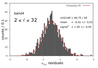
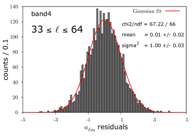
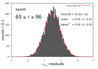
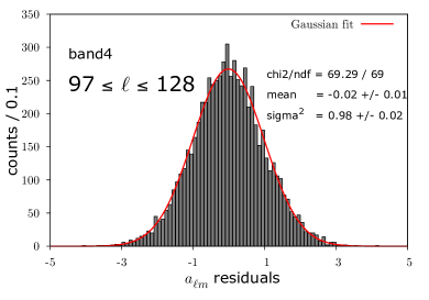
Figure 7.— Distribution of 2MASS band 4 map residuals in harmonic space, according to Equation (21), for different ranges of multipoles $\ell$ and a variance model given by $\sigma^{2}=f_{sky}B_{\ell}^{2}C_{\ell}+\eta$. The variance $C_{\ell}$ is taken from the fiducial $\Lambda$CDM model, with nonlinearities in the LSS given by CAMB’s halofit implementation (see Section 6 for details). The effect of the mask is partially corrected by rescaling the $C_{\ell}$ values by an $f_{\text{sky}}$ factor, and the pixelization is also taken into account. Shot noise is included in the total variance, and the bias factor $b_{g}$ was taken by fitting this model to the the survey power spectrum in the region $2\leq\ell\leq 50$ (see Table 3). The decomposed map has $nside=64$, and no beaming, except for the pixelization, has been applied. Gaussian fits are shown on top of each histogram.

In order to apply the method of Section 4 to the CMB–galaxy cross-correlation, we first need to test whether the hypothesis of Gaussianity is, at least approximately, respected in harmonic space by the distribution of $a_{\ell m}$ coefficients. Especially at small scales, it is hard to predict the nature of the fluctuations of these coefficients in the nonlinear regime. In pixel space, lognormality as an approximate property of the galaxy count distributions in 2-dimensional cells was first observed by Hubble (1934). This was proposed as a model when Coles & Jones (1991) showed that such a distribution could be obtained from a purely Gaussian field through gravitational evolution. Figure 6 displays the distributions of the 2MASS galaxy counts per pixel and evinces that, as the density of galaxies per pixel increases, the distributions tend to lognormal. However, one can see that for 2MASS statistics, even for band 4 with about 13 galaxies pixels^-1 on average, the $\chi^{2}/n$ dof is still bad. Figure 7 shows the distribution of the harmonic space residuals

$$a_{\ell m}\textrm{ residuals}=\left\{\begin{array}[]{ll}\sqrt{2}\textrm{Re}(a_{\ell m})/\sigma&\quad(m\neq 0)\\ \sqrt{2}\textrm{Im}(a_{\ell m})/\sigma&\quad(m\neq 0)\\ \textrm{Re}(a_{\ell m})/\sigma&\quad(m=0),\end{array}\right.$$ (21)

for 2MASS band 4, considering as a model for the total variance $\sigma^{2}=f_{sky}B_{\ell}^{2}C_{\ell}+\eta$, with shot noise $\eta$ taken into account (see Table 3). The $C_{\ell}$ values have been taken from a $\Lambda$CDM cosmology and a suitable galaxy bias parameter to describe the pseudo-power spectrum (corrected by $f_{\text{sky}}$) for this band (see Section 6 for details). The $a_{\ell m}$ values are the partial-sky pseudo-coefficients in harmonic space. The panels present the $a_{\ell m}$’s histograms in four different multipole ranges. We can see that, except for the range $65\leq\ell<96$, fluctuations in harmonic space are fairly well described by zero-mean, unit-variance Gaussians at the $1\sigma$ level, even though the (co) variance model used is simple, not including the mixture induced by the mask, but a simple scale-independent $f_{\text{sky}}$ correction. The distributions for the other three bands are similar to those for band 4. To avoid aliasing for multipoles as large as $\ell_{max}=128$ in these plots, the resolution parameter for the contrast map was taken to be a bit larger ($nside=64$) than the final map resolution used in the Gibbs chains ($nside=32$). We stress that the Gaussianity of fluctuations seen in harmonic space is not at all inconsistent with the histograms of galaxy counts in pixel space of Figure 6. The statistical properties of the $a_{\ell m}$ depend on the $n$-point correlation functions. For example, their variances ($C_{\ell}^{gg}$) are related to the two-point angular autocorrelation function $w(\theta)$ by

$$w(\theta)=\sum_{\ell}\frac{2\ell+1}{4\pi}C_{\ell}^{gg}P_{\ell}(\cos\theta),$$ (22)

and therefore are not determined simply by the distribution of galaxy counts, but by how these counts are correlated at a given angular scale. At each bin of the histograms in Figure 6, several different angular scales are mixed, and the information on the correlation at each scale is lost. It is also important to say that the aspect of the histograms of Figure 7 does not prove complete Gaussianity of the spherical harmonics of 2MASS contrast maps, since small non-Gaussianities should be probed with more sensitive estimators like the bi-spectrum, for example.

6. Validating the Bayesian method

We validated the methodology described so far via the MC approach. For this, we adopted $\Lambda$CDM as the fiducial model, with the cosmological parameter values listed in Table 1. We have obtained the power spectrum $C_{\ell}^{tt}$ for the CMB temperature fluctuations and the 3D matter power spectrum $P(k)$ at large scales, taking into account nonlinear effects in the structure formation, using the CAMB (Lewis et al., 2000; Lewis & Bridle, 2002; Howlett et al., 2012; Lewis, 2013) + HALOFIT (Takahashi et al., 2012) code.

We have then used $P(k)$ to build the corresponding galaxy autocorrelation spectrum $C_{\ell}^{gg}$ and the temperature–galaxy cross-correlation spectrum $C_{\ell}^{tg}$ by assuming a linear galaxy bias $b_{g}$. In order to mitigate the bias to be introduced by such a linearity hypothesis, even at scales below about $10\ h^{-1}$ Mpc where collapsed halos start to dominate, we fitted $b_{g}$ to the 2MASS autocorrelation angular power spectrum considering just multipoles no larger than $\ell=50$ (intermediate scales). The corresponding selection functions for each of the four 2MASS magnitude bands were also included (see Table 2). Figure 8 shows data versus theory comparisons, accounting for the $b_{g}$ best-fitting values (displayed on Table 3) in the 2MASS linear (red line) and nonlinear (blue line) spectra. The data point central values were obtained by decomposing the masked galaxy contrast map into spherical harmonics with HEALPix routines, and then rescaled by a scale factor $1/f_{\text{sky}}$, to partially correct for the power loss introduced by the mask, and also by the power dump introduced by the pixelization at small scales. Finally, shot noise (given by $1/\overline{N}$, where $\overline{N}$ is the average number of galaxies per steradian) was also subtracted from the data. Figure 8 also evinces another reason for using a broad $5^{\circ}$ beam, even for the galaxy contrast map: both the CMB and galaxy original maps are not bandwidth limited in the region $\ell\buildrel<\over{\sim}96$, so that spherical harmonics decompositions using low-resolution ($nside=32$) unbeamed maps would be severely affected by aliasing, especially in the multipole range $64\buildrel<\over{\sim}\ell\buildrel<\over{\sim}96$. Moreover, to keep integration errors under control in the high-$\ell$ region, all decompositions have been performed with at least four iterations with HEALPix routines.

In linear theory, the autocorrelation matter power spectrum normalization depends on the product $\sigma_{8}b_{g}$. Here we have chosen to fit $b_{g}$ fixing $\sigma_{8}$ at 0.78. For comparison, fitting all four 2MASS-XSC bands together (using $\Omega_{m}=0.30$, $\Omega_{b}=0.05$, $\sigma_{8}=0.75$ and $h=0.7$) in the range $\ell=1-50$, Rassat et al. (2007) found $b_{g}=1.40\pm 0.03$. Binning multipoles, Afshordi et al. (2004) fitted each band separately and found that the biases for the different magnitude bands lie within $b_{g}=1.18\pm 0.08$ for $\ell\buildrel<\over{\sim}70$.

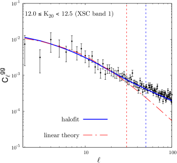
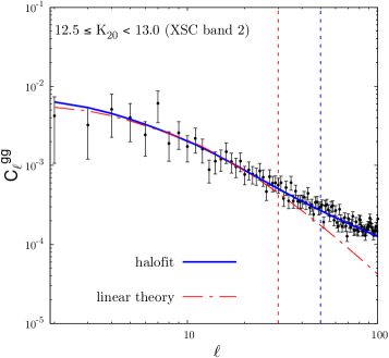
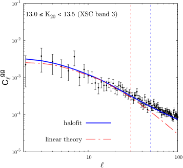
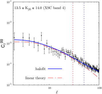
Figure 8.— Data vs. theory comparisons for the galaxy autocorrelation power spectrum $C_{\ell}^{gg}$. The dark matter power spectrum was scaled to data by fitting the galaxy bias factor $b_{g}$ (see Table 3 for the best-fitting values and errors for each of the 2MASS magnitude bands). The vertical lines mark the maximum multipole $\ell$ used in the fit. Both a pure linear model (red) and a model with nonlinearities given by CAMB’s HALOFIT implementation (blue) are shown. Shot noise has been subtracted from the data.

Table 3Results of the fit for the four 2MASS bands of the bias parameter $b_{g}$.

		Linear ($\ell_{max}=30$)		Halofit ($\ell_{max}=50$)		Halofit ($\ell_{max}=96$)
Band	Shot Noise	$b_{g}\pm\sigma_{b}$	$\chi^{2}$/ndof	$b_{g}\pm\sigma_{b}$	$\chi^{2}$/ndof	$b_{g}\pm\sigma_{b}$	$\chi^{2}$/ndof
1	$1.8\times 10^{-4}$	$1.27\pm 0.04$	19.1/28	$1.32\pm 0.02$	33.5/48	$1.37\pm 0.01$	127.3/94
2	$8.5\times 10^{-5}$	$1.25\pm 0.03$	17.3/28	$1.34\pm 0.03$	29.2/48	$1.35\pm 0.01$	102.1/94
3	$4.0\times 10^{-5}$	$1.22\pm 0.03$	16.9/28	$1.29\pm 0.02$	37.3/48	$1.34\pm 0.01$	86.2/94
4	$1.9\times 10^{-5}$	$1.18\pm 0.03$	32.2/28	$1.28\pm 0.02$	52.5/48	$1.29\pm 0.01$	105.9/94

Note: Both a pure linear model and one with nonlinearities (HALOFIT) are shown, as well as $\ell_{max}$ used in each fit.

Once $b_{g}$ has been estimated, a combined realization of a CMB temperature map ($nside=512$) and 2MASS galaxy contrast map ($nside=64$) was produced, including their cross-correlation signal. A $5^{\circ}$ Gaussian beam was applied to both maps, and their resolutions were degraded to $nside=32$. Finally, white noise of RMS strength $\sigma_{0}=2\ \mu$K pixel^-1 was added to the CMB low-resolution map and of $5\%$ pixel^-1 to the galaxy contrast map. Such noise levels dominate the power in both maps for scales above $\ell=60$, as can be seen in Figures 9 and 10, where the full-sky $tt$ and $gg$ power spectra were retrieved from the input maps, respectively.

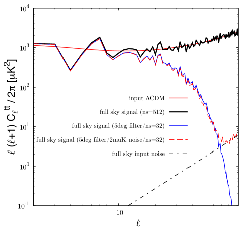
Figure 9.— CMB autocorrelation power spectra: input $\Lambda$CDM (red solid line), full-sky spectrum for a given CMB map realization at $nside=512$ (black solid line), spectrum convoluted with a $5^{\circ}$ Gaussian beam and sampled at $nside=32$ (blue solid line), spectrum after the addition of 2$\mu$K pixel^-1 RMS white noise (dashed red line), and added noise power (dashed black line).

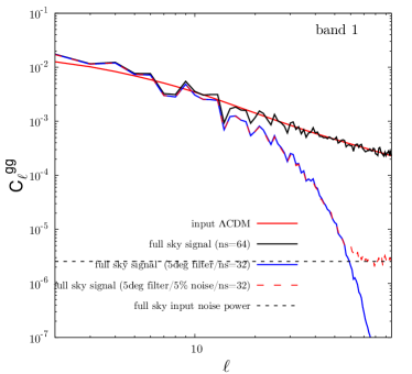
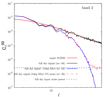
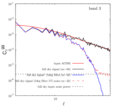
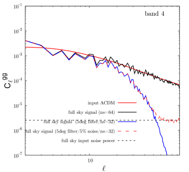
Figure 10.— Galaxy contrast autocorrelation power spectra for the four 2MASS selection functions: input $\Lambda$CDM with biases given in Table 3 (red solid line), full-sky spectrum for a given galaxy contrast map realization at $nside=64$ (black solid line), spectrum convoluted with a $5^{\circ}$ Gaussian beam and sampled at $nside=32$ (blue solid line), spectrum after the addition of 5% pixel^-1 RMS white noise (dashed red line), and added noise power (dashed black line).

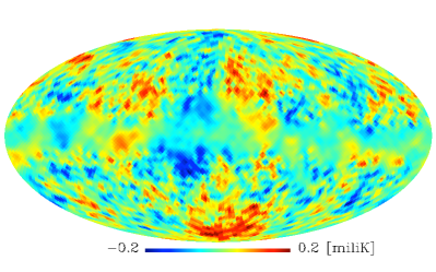
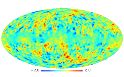
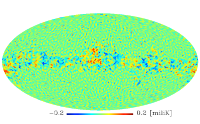
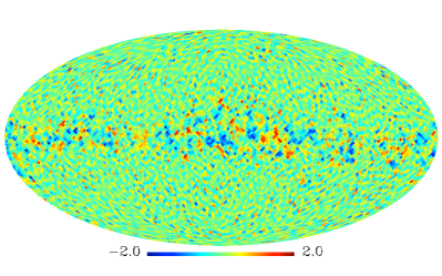
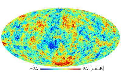
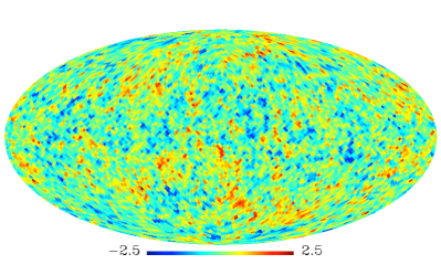
Figure 11.— Sky maps associated with the Gibbs chain sampled fields. Left: CMB temperature field. Right: galaxy contrast field. Top: mean field $\boldsymbol{x}$. Middle: fluctuation field $\boldsymbol{y}$; Bottom: total field $\boldsymbol{x}+\boldsymbol{y}$. The corresponding 2MASS selection function is that of band 1.

The four sets of combined CMB/contrast maps (one for each of the 2MASS selection functions) described above were then used to feed a Gibbs chain, whose sampling equations were described in Section 4. The mask used was the combination of 2MASS and WMAP9 masks described in Section 5, with a final sky fraction of $f_{\text{sky}}=0.70$. The initial state of the chain was chosen to be the full covariance matrix of the fiducial model itself. The monopole and dipole, both null for the fiducial spectrum, were kept fixed at these values along the whole chain. Multipoles were sampled up to $\ell_{max}=51$, and kept fixed for $51<\ell\leq 96$ at the fiducial model spectra. For $\ell>96$, the spectrum was taken to be zero. We also have used the Jeffreys scale-invariant prior, $\pi(\mathbf{S})=|\mathbf{S}|^{-1}$ (Wandelt et al., 2004).

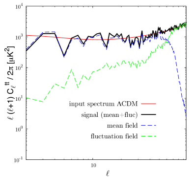
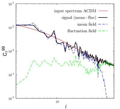
Figure 12.— Autocorrelation power spectrum of the Gibbs chain fields of Figure 11. The total ($\boldsymbol{x}+\boldsymbol{y}$), mean ($\boldsymbol{x}$), and fluctuation ($\boldsymbol{y}$) fields are shown separately.

Even though the initial spectrum was already at its true state, a burn-in phase of 100 samples was considered, and all the samples drawn after this initial phase were used for statistical analysis, that is, we have ignored possible correlations between adjacent samples of the chain. A total of 50,000 samples for each 2MASS selection function were generated using 50 independent parallel chains. Figure 11 shows the sky maps associated with the fields of Equation (16) (the mean field $\boldsymbol{x}$, the fluctuation field $\boldsymbol{y}$ and the total field $\boldsymbol{x}+\boldsymbol{y}$) for one of the band 1 realizations. Some of the statistical properties of these fields can be seen in Figure 12, where the autocorrelation power spectrum of each component is displayed separately. One sees that at large scales ($\ell\buildrel<\over{\sim}10$) the total field is dominated by its mean component $\boldsymbol{x}$, whereas at small scales ($\ell\buildrel>\over{\sim}60$), where the added uncorrelated white noise is larger than the primordial signal, the total field is dominated by $\boldsymbol{y}$. Another interesting feature of these random fields is the behavior of the autocorrelation at large scales for the fluctuation $\boldsymbol{y}$. According to Equation (16), the small-$\ell$ region is characterized by a large S/N ($S/N\gg 1$), so the covariance of $\boldsymbol{y}$ in harmonic space is approximately $\mathbf{B}^{\textrm{\tiny{-2}}}\mathbf{N}$:

$$\mathbf{C(\boldsymbol{y})}=E(\boldsymbol{y}\otimes\boldsymbol{y})\stackrel{{\scriptstyle S/N\gg 1}}{{\simeq}}\mathbf{B}^{-2}\mathbf{N}.$$ (23)

Neglecting the effect of the beam at these scales, the autocorrelations are quite different from those of the added full-sky noise (see Figures 9 and 10). This is the direct effect of the mask whose mixing effect distorts also the noise (see Equation (18)).

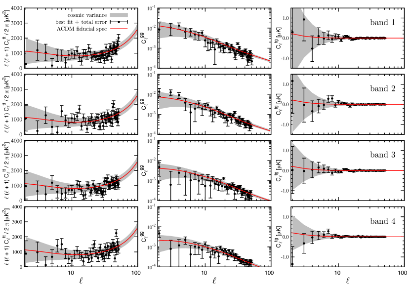
Figure 13.— Monte Carlo. Best-fit values (dots with error bars) are shown for the full covariance matrix of a combined CMB–LSS experiment. Central values are the maximum of a log-likelihood Blackwell–Rao estimator, and the error bars contain contributions from experimental noise and cosmic variance (also shown separately as a gray band) around a fiducial $\Lambda$CDM (red line) model (see Greason et al. (2012) for details).

With the 50,000 available samples, we have reconstructed a likelihood for this combined CMB–LSS data set using a Blackwell–Rao estimator (Chu et al., 2005; Dunkley et al., 2009). For a certain number of Gibbs samples $n_{G}$, we were able to find an analytic solution for the maximum of the log-likelihood (see Appendix A), which allowed us to construct the best-fitting spectra shown in Figure 13. The error bars were estimated assuming Gaussian errors, and the cosmic variance band was calculated taking the $\Lambda$CDM fiducial model as reference (see Greason et al. (2012) for details). While useful for many purposes, these central values with their associated errors should only be taken as a first approximation to the full (and non-Gaussian) likelihood function close to its maximum.

Table 4Summary of All parameters/maps/choices used to run the Gibbs chain

Parameter	Choice
Input maps	ILC/$Q$/$V$/$W$ 9 years (r9)
Beaming	Effective $5^{\circ}$ (FWHM)
CMB noise level	2$\mu$K pixel-1 (RMS)
Galaxy contrast noise level	5% pixel-1 (RMS)
Mask	Combined KQ85y9 $\times$ 2MASS (r5)
Final maps resolution	r5 ($nside=32$)
Input spectrum	$\Lambda$CDM best-fit to WMAP9
Sampling mode	COMMANDER
Preconditioner	block-diagonal
Monopole/dipole	fixed (float. dipole)
Maximum multipole	$\ell_{max}=96$
Start of fiducial spectrum	$\ell=52$
Prior	Jeffrey (flat)
Burn-in phase	100 (500) samples
Skipped samples	0 (1)
CG convergence	$10^{-6}$

7. Application to the WMAP–2MASS combined data set

In Section 6 we used a fiducial power spectrum where $C_{0}^{tt}=C_{1}^{tt}=0$. In order to apply this approach to real data, we had to follow a slightly different procedure. Although the monopole and dipole terms are removed in the input WMAP9 maps and their residual values are small in comparison to other multipoles at large scale, we verified that they could not be fixed at zero. Otherwise, the Gibbs chains converge to anomalous states at those scales. Thus, decomposing the ILC, Q, V and W maps with partial sky coverage, we obtained estimates for $C_{0}^{tt}$ and $C_{1}^{tt}$. We used these estimates to perform the analyses, keeping them fixed along the chain. With the block-diagonal preconditioner of Equation (17), the average number of iterations required to solve the linear systems of Equations (15) and (16) was about 700 for all 2MASS bands. This is still a reasonable number for the map resolutions adopted here, but if a finer pixelization is required, one needs to seek for better preconditioners, like those used by Eriksen et al. (2004) and Oh et al. (1999) for example.

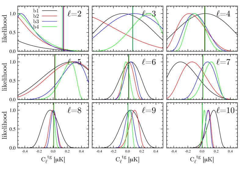
Figure 14.— One-dimensional slices of the Blackwell–Rao likelihood (normalized to 1 in its peak) built from 50,000 Gibbs samples. Nine slices are shown, corresponding to the first $C_{\ell}^{tg}$ multipoles, where all but the multipole being plotted are kept fixed at their maximum log-likelihood values. The different colors identify each of the four 2MASS selection functions (bands) considered in this work. Vertical lines show the expected values from a $\Lambda$CDM model.

Figure 14 shows a few ($2\leq\ell\leq 10$) one-dimensional slices of the Blackwell–Rao likelihood for the cross-correlation $C_{\ell}^{tg}$, where all but the multipole in the horizontal axis are fixed at their maximum log-likelihood values. Similar to the results with MC samples, one sees that for a shallow survey like 2MASS, the cross-correlation signal, if present, is always plunged into a region of large cosmic variance. We stress here, however, that this might not be the case if the cross-correlation signal is probed with deeper selection function surveys.

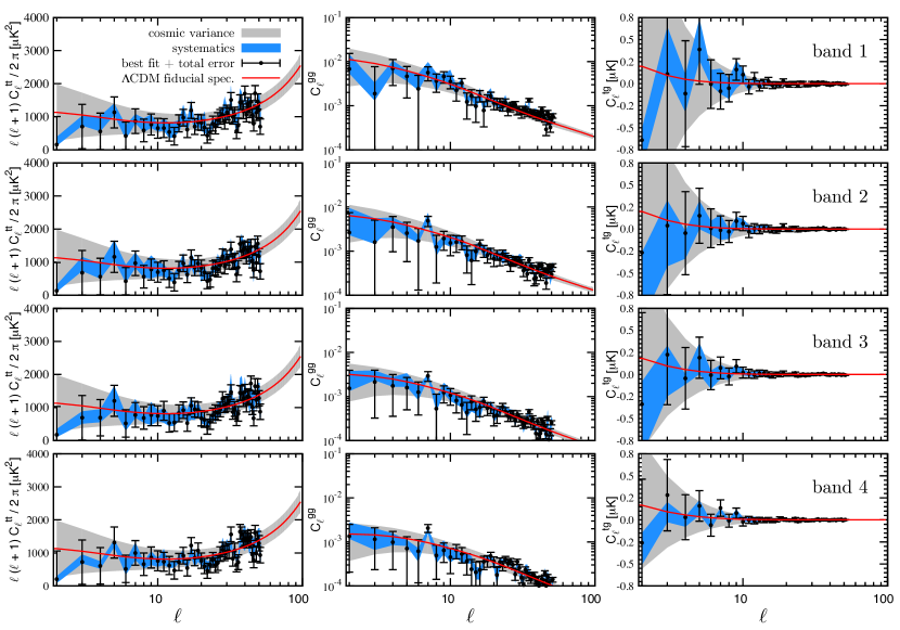
Figure 15.— The systematic blue band is bounded by the maximum and minimum values of best-fit multipole values obtained using different Gibbs chains fed with $W$ channel-2MASS and ILC-2MASS maps (see text of Section 7 for details). Cosmic variance around a $\Lambda$CDM fiducial model (red line) is also shown as a gray band. Data points with error bars are the weighted average for channels $Q$, $V$ and $W$ with weights given by the reciprocal of noise variances.

In Figure 15, we show the result of the weighted average best-fit spectra of 2MASS $\times$ Q, V, W channels (using the reciprocal of the noise variance as weight), together with the corresponding bands of cosmic variance (gray) around the fiducial $\Lambda$CDM model. As already largely discussed in the literature, we also find a low value for the CMB quadrupole $C_{2}^{tt}$ . The smallness of the quadrupole has already been shown to be consistent with the level of cosmic variance fluctuations at large angular scales (Efstathiou, 2003a, b; de Oliveira-Costa et al., 2004).

In order to have an estimate of the systematic uncertainties coming from the Gibbs sampling algorithm, we have run the Gibbs chains slightly differently than in the fiducial case shown in Table 4 taking the WMAP9 $W$ channel and ILC as templates, namely:

1. a flat prior was used for the spectrum;

2. a larger burn-in phase was tested by throwing away the first 500 samples of each chain;

3. possible correlations between adjacent samples were probed by skipping one of every two samples of the chain.

The typical level of variation obtained in the final values of the maximum of the log-likelihood is represented by the blue bands in Figure 15. The use of the ILC map in building these bands provides a rough estimate on possible residual foregrounds at high galactic latitudes. One can see that at large scales, where the signal from the ISW effect is expected to be present in an accelerated universe, the most important source of uncertainty is still cosmic variance. It is worth mentioning that the blue bands of Figure 15 cannot be taken as the full systematic uncertainties, since we only investigated a few contributions coming from the Bayesian approach adopted here and possible foregrounds. A more robust estimate of systematics affecting the temperature maps, such as those introduced by residual foregrounds at high latitudes, for example, will be obtained by applying the same methodology to the independent temperature sky maps measured by the Planck satellite.

8. Conclusions

The ISW signal, a temperature anisotropy induced by time-varying gravitational potentials in an accelerated universe, is a powerful tool to probe the DE properties and break the degeneracy among competing theoretical models. From the observational point of view, the scientific community has been gifted by a number of outstanding results from different instruments, improving the understanding of the properties of both CMB and large-scale distribution of matter in our local universe.

In this work we explored the potential of the cross-correlation between the CMB temperature fluctuations and the LSS as a probe for the ISW effect, with data coming, respectively, from the WMAP9 data release and the 2MASS infrared galaxy catalog. The cross-correlation signal has been estimated by maximizing the likelihood for observing the combined WMAP9–2MASS data sets, using a Gibbs sampling technique in order to reconstruct the likelihood without a direct (and computationally expensive) evaluation of it, in either pixel or harmonic space. The four 2MASS selection functions considered here lead to a shallow sampling of LSS distribution and, in turn, to a cross-correlation signal severely affected by cosmic variance. The role of such an intrinsic fluctuation on the cross-spectrum was also studied by tracking the convergence of a MASTER solution (as an ensemble average over a certain number of sky realizations) toward its true value. The analysis pipeline, however, was successfully validated using MC control samples and can be easily applied to current deeper surveys, such as the SDSS (Alam et al., 2015) or the Dark Energy Survey (DES; DES Collaboration (2005)), as well as to future data coming from the Large Synoptic Survey Telescope (LSST; LSST Science Collaboration (2013)). Ongoing efforts of the authors will compare the current results with those obtained using CMB maps produced by the Planck satellite.

An initial estimate of the systematic uncertainty associated with the sampling algorithm and possible foregrounds was also obtained and turned out to be a subdominant contribution to the total uncertainty when compared to cosmic variance. We also tested the behavior of the method in the presence of a higher cross-correlation signal, more precisely, five times larger than expected in the $\Lambda$CDM model. In such a scenario, we verified that, for a 2MASS-like survey, the statistical significance of the cross-correlation signal is still limited by cosmic variance. However, as can be seen from the analysis performed with MC samples, when enough signal is present at smaller scales, where the noise, and not the irreducible cosmic variance, is the dominant source of uncertainty, the Bayesian method is able to recover the true signal. In Zhao et al. (2009) and Hojjati et al. (2011), for example, suitable general modifications of the equations governing the growth of cosmological perturbations were presented, allowing for the auto- and cross-correlation power spectra of CMB and LSS to be calculated within a modified version of CAMB. The spectra for a few modified gravity models diverge from that of general relativity from intermediate to small angular scales ($\ell\buildrel>\over{\sim}20$). Such departures could be scrutinized with the methods presented in this paper, as long as maps of higher resolution than the ones used here and better preconditioners are fed into the Gibbs chains. Therefore, we believe that the methodology described in this paper would be able to help solve existing issues in the field of ISW measurements, and we hope that it will become a complementary tool for the current studies of DE and modified gravity.

9. Acknowledgements

This publication makes use of data products from 2MASS, which is a joint project of the University of Massachusetts and the Infrared Processing and Analysis Center/California Institute of Technology, funded by the National Aeronautics and Space Administration and the National Science Foundation.

For the use of the 2MPZ catalog (Bilicki et al., 2014) we acknowledge the Wide Field Astronomy Unit.

The authors acknowledge the use of the Legacy Archive for Microwave Background Data Analysis (LAMBDA), part of the High Energy Astrophysics Science Archive Center (HEASARC). HEASARC/LAMBDA is a service of the Astrophysics Science Division at the NASA Goddard Space Flight Center.

Some of the results in this paper have been derived using the HEALPix package (Gorski et al., 2005).

E.M.-S. and M.P.-L. acknowledge the use of the University of São Paulo (USP) cloud computing environment InterNuvem USP. F.C.C. was supported by FAPERN/PRONEM and CNPq and acknowledges the use of the University of State of Rio Grande do Norte computing cluster. M.P.-L. thanks CNPq (PCI/MCTI/INPE program and grant 202131/2014-9) for financial support. C.P.N. thanks CAPES for financial support and the use of the COAA/ON cluster. C.A.W. and E.M.-S. were partially supported by CNPq grants 313597/2014-6 and 309452/2012-0, respectively.

Finally, the authors would like to thank the referee for the careful reading of the manuscript and valuable comments that contributed to the improvement of the paper.

Appendix A Analytical solution for the maximum of a Blackwell–Rao log-likelihood

We present here an analytic solution to the maximum of the logarithm of a Blackwell–Rao estimator.

For a block-diagonal matrix $\mathbf{S}$, whose $2\times 2$ submatrices are $\mathbf{S}_{\ell}$ (given in Equation (12)), its posterior probability distribution can be written as product of the prior $\pi(\mathbf{S})=|\mathbf{S}|^{-q}$ to the $2\ell+1$ degrees of freedom inverse-Wishart distribution (Gupta & Nagar, 1999):

$$P(\mathbf{S}|\mathbf{s})\propto\pi(\mathbf{S})\prod_{\ell}\frac{1}{2^{\frac{2\ell-2}{2}}\Gamma_{2}\left(\frac{2\ell-1}{2}\right)}\frac{|\bm{\sigma}_{\ell}|^{\frac{2\ell-2}{2}}}{|\mathbf{S}_{\ell}|^{\frac{2\ell+1}{2}}}\exp\left[-\frac{1}{2}\textrm{Tr}\left(\bm{\sigma}_{\ell}\mathbf{S}_{\ell}^{-1}\right)\right].$$ (A1)

Neglecting the terms that do not depend on $\mathbf{S}_{\ell}$, we can write the logarithm of the posterior as

$$\textrm{ln}P=-\frac{1}{2}\sum_{\ell}\left[(2\ell+1+2q)\textrm{ln}|\mathbf{S}_{\ell}|+\textrm{Tr}\left(\bm{\sigma}_{\ell}\mathbf{S}_{\ell}^{-1}\right)\right]$$ (A2)

and, for $n_{G}$ Gibbs samples represented by the total signal power matrices $\bm{\sigma}_{\ell}^{(n)}$ ($n=1,...,n_{G}$), an estimate of the Blackwell–Rao log-likelihood is given by

$$\textrm{ln}\mathscr{L}=\frac{1}{n_{G}}\sum_{n}\textrm{ln}P_{n}=-\frac{1}{2}\sum_{\ell}(2\ell+1+2q)\textrm{ln}|\mathbf{S}_{\ell}|-\frac{1}{2}\frac{1}{n_{G}}\sum_{n}\sum_{\ell}\textrm{Tr}\left(\bm{\sigma}_{\ell}^{(n)}\mathbf{S}_{\ell}^{-1}\right),$$ (A3)

whose maximum,

$$\frac{\partial}{\partial C_{\ell}}\textrm{ln}\mathscr{L}=0\quad(0\leq\ell\leq\ell_{max}),\quad C_{\ell}=C_{\ell}^{tt},C_{\ell}^{gg},C_{\ell}^{tg},$$ (A4)

provides

$$\frac{\partial}{\partial C_{\ell}}\textrm{ln}\mathscr{L}=-\frac{1}{2}\frac{\partial}{\partial C_{\ell}}\textrm{ln}|\mathbf{S}_{\ell}|-\frac{1}{2}\frac{1}{n_{G}}\sum_{n}\frac{\partial}{\partial C_{\ell}}\textrm{Tr}\left(\bm{\sigma}_{\ell}^{(n)}\mathbf{S}_{\ell}^{-1}\right).$$ (A5)

Denoting the average over Gibbs samples as $\overline{\alpha}=\sum_{n}\alpha_{n}$ and using the relation

$$\overline{\textrm{Tr}\left(\bm{\sigma}_{\ell}\mathbf{S}_{\ell}^{-1}\right)}=\textrm{Tr}\left(\overline{\bm{\sigma}}_{\ell}\mathbf{S}_{\ell}^{-1}\right),$$ (A6)

we can write the following set of three coupled equations:

$$C_{\ell}^{tt}\left[\textrm{Tr}\left(\overline{\bm{\sigma}}_{\ell}\mathbf{S}_{\ell}^{-1}\right)-(2\ell+1+2q)\right] = \overline{\sigma}_{11}$$ (A7)

$$C_{\ell}^{gg}\left[\textrm{Tr}\left(\overline{\bm{\sigma}}_{\ell}\mathbf{S}_{\ell}^{-1}\right)-(2\ell+1+2q)\right] = \overline{\sigma}_{22}$$ (A8)

$$C_{\ell}^{tg}\left[\textrm{Tr}\left(\overline{\bm{\sigma}}_{\ell}\mathbf{S}_{\ell}^{-1}\right)-(2\ell+1+2q)\right] = \overline{\sigma}_{12},$$ (A9)

whose solution is given by

$$\mathbf{S}_{\ell}=\frac{1}{2\ell+1+2q}\overline{\bm{\sigma}}_{\ell}=\frac{1}{2\ell+1+2q}\left(\begin{array}[]{cc}\overline{\sigma}_{11}&\overline{\sigma}_{12}\\ \overline{\sigma}_{12}&\overline{\sigma}_{22}\end{array}\right).$$ (A10)

References

- Afshordi et al. (2004) Afshordi, N., Loh, Y.-S., & Strauss, M. A. 2004, PRD, 69, 083524
- Abazajian et al. (2009) Abazajian, K. N., Adelman-McCarthy, J. K., Agüeros, M. A., et al. 2009, ApJS, 182, 543
- Alam et al. (2015) Alam, S., Albareti, F. D., Allende Prieto, C., et al. 2015, ApJS, 219, 12
- Betoule et al. (2014) Betoule, M., Kessler, R., Guy, et al. 2014, A&A, 568, A22
- Bennett et al. (2013) Bennett, C. L., Larson, D., Weiland, J. L., et al. 2013, ApJS, 208, 20
- Bilicki et al. (2014) Bilicki et al. 2014, ApJS, 210, 9
- Bond (1998) Bond, J. R., Jaffe, A. H., Knox, & L. 1998, PRD, 57, 2117
- Boughn & Crittenden (2002) Boughn, S. P., & Crittenden, R. G. 2002, PRL, 88, 021302
- Boughn & Crittenden (2004a) Boughn, S. P., & Crittenden, R. G. 2004a, ApJ, 612, 647
- Boughn & Crittenden (2004b) Boughn, S. P., & Crittenden, R. G. 2004b, Nature, 427, 45
- Boughn & Crittenden (2005a) Boughn, S. P., & Crittenden, R. G. 2005a, NewAR, 49, 75
- Boughn & Crittenden (2005b) Boughn, S. P., & Crittenden, R. G. 2005b, MNRAS, 360, 1013
- Bull et al. (2015) Bull, P., Wehus, I. K., Eriksen, H. K., et al. 2015, ApJS, 219, 10
- Cabre et al. (2006) Cabre, A., Gaztanaga, E., Manera, M., Fosalba, P., & Castander, F. 2006, MNRAS, 372, L23
- Carvalho et al. (2006) Carvalho, F. C., Alcaniz, J. S., Lima, J. A. S., & Silva, R. 2006, PRL, 97, 081301
- Chu et al. (2005) Chu, M., Eriksen, H. K., Knox, L., et al. 2005, PRD, 71, 103002
- Coles & Jones (1991) Coles, P, & Jones, B. 1991, MNRAS, 248, 1
- Copeland et al. (2006) Copeland, E. J., Sami, M., & Tsujikawa, S. 2006, IJMPD, D15, 1753
- Cooray (2002) Cooray, A. 2002, PRD, 65, 103510
- Crittenden & Turok (1996) Crittenden, R. G., & Turok, N. 1996, PRL, 76, 575
- de Oliveira-Costa et al. (2004) de Oliveira-Costa, A., Tegmark, M., Zaldarriaga, M., & Hamilton, A. 2004, PRD, 69, 063516
- DES Collaboration (2005) DES Collaboration 2005, The Dark Energy Survey, http://adsabs.harvard.edu/abs/2005astro.ph.10346T
- Dunkley et al. (2009) Dunkley, J., Spergel, D. N., Komatsu, E., et al. 2009, ApJ, 701, 1804
- Dupé et al. (2011) Dupé, F.-X., Rassat, A., Starck, J.-L., & Fadili, M. J. 2011, A&A, 534, A51
- Efstathiou (2003b) Efstathiou, G. 2003b, MNRAS, 343, L95
- Efstathiou (2003a) Efstathiou, G. 2003a, MNRAS, 346, L26
- Eriksen et al. (2004) Eriksen, H. K., O’Dwyer, I. J., Jewell, J. B., et al. 2004, ApJS, 155, 227
- Ferraro et al. (2015) Ferraro, S., Sherwin, B. D., Spergel, D. N. 2015, PRD, 91, 083533
- Fosalba et al. (2003) Fosalba, P., Gaztanaga, E., & Castander, F. 2003, ApJ, 597, L89
- Fosalba & Gaztanaga (2004) Fosalba, P., & Gaztanaga, E. 2004, MNRAS, 350, L37
- Gaztanaga et al. (2006) Gaztanaga, E., Manera, M., & Multamaki, T. 2006, MNRAS, 365, 171
- Giannantonio et al. (2006) Giannantonio, T., Crittenden, R. G., Nichol, R. C., et al. 2006, PRD, 74, 063520
- Giannantonio et al. (2012) Giannantonio, T., Crittenden, R., Nichol, R., & Ross, A. J. 2012, MNRAS, 426, 2581
- Giannantonio et al. (2014) Giannantonio, T., Ross, A. J., Percival, W. J., et al. 2014, PRD, 89, 023511
- Gorski et al. (2005) Gorski, K. M., Hivon, E., Banday, A. J., et al. 2005, ApJ, 622, 759
- Goto et al. (2012) Goto, T., Szapudi, I., Granett, B. R. 2012, MNRAS, 422, L77
- Granett et al. (2008) Granett, B. R. and Neyrinck, M. C. and Szapudi, I. 2008, ApJL, 683, L99
- Granett et al. (2015) Granett, B. R., Kovács, A., & Hawken, A. J. 2015, MNRAS, 454, 2804
- Greason et al. (2012) Greason, M. R., Limon, M., Wollack, E., et al. 2012, Nine-Year Wilkinson Microwave Anisotropy Probe (WMAP) Observations: Nine Year Explanatory Supplement, http://lambda.gsfc.nasa.gov
- Gupta & Nagar (1999) Gupta, A.K., & Nagar, D.K. 1999, Matrix Variate Distributions (Chapman and Hall/CRC)
- Hernández-Monteagudo et al. (2014) Hernández-Monteagudo, C. Ross, A. J., Cuesta, A., et al. 2014, MNRAS, 438, 1724
- Hinshaw et al. (2013) Hinshaw, G., Larson, D., Komatsu, E., et al. 2013, ApJS, 208, 19
- Hivon et al. (2002) Hivon, E., Gorski, K. M., Netterfield, C. B., et al. 2002, ApJ, 567, 2
- Ho et al. (2008) Ho, S., Hirata, C., Padmanabhan, N., Seljak, U., & Bahcall, N. 2008, PRD, 78, 043519
- Hobson (2010) Hobson, M.P. 2010, Bayesian Methods in Cosmology (Cambridge: Cambridge University Press)
- Hojjati et al. (2011) Hojjati, A., Pogosian, L. & Zhao, G.-B. 2011, JCAP, 8, 005
- Howlett et al. (2012) Howlett, C., Lewis, A., Hall, A., & Challinor, A. 2012, JCAP, 1204, 027
- Hubble (1934) Hubble, E. 1934, ApJ, 79, 8
- Jewell et al. (2004) Jewell, J., Levin, S., & Anderson, C. H. 2004, ApJ, 609, 1
- Joyce et al. (2015) Joyce, A., Jain, B., Khoury, J., & Trodden, M. 2015, PR, 568, 1
- Kamionkowski (1996) Kamionkowski, M. 1996, PRD, 54, 4169
- Kinkhabwala & Kamionkowski (1999) Kinkhabwala, A., & Kamionkowski, M. 1999, PRL, 82, 4172
- Kinkhabwala & Kamionkowski (1999) Kinkhabwala, A., & Kamionkowski, M. 1999, PRL, 82, 4172
- Larson et al. (2007) Larson, D. L., Eriksen, H. K., Wandelt, B. D., et al. 2007, ApJ, 656, 653
- Lewis (2013) Lewis, A. 2013, PRD, 87, 103529
- Lewis & Bridle (2002) Lewis, A., & Bridle, S. 2002, PRD, 66, 103511
- Lewis et al. (2000) Lewis, A., Challinor, A., & Lasenby, A. 2000, ApJ, 538, 473
- LSST Science Collaboration (2013) LSST Science Collaboration, Ivezić, Ž., et al. 2013, LSST Science Requirements Document, http://ls.st/LPM-17
- McEwen et al. (2007) McEwen, J. D., Vielva, P., Wiaux, Y., et al. 2007, J. Fourier Anal. Appl., 13, 495
- Nadathur et al. (2012) Nadathur, S., Hotchkiss, S., Sarkar, S. 2012, JCAP, 2012, 042
- Nojiri & Odintsov (2011) Nojiri, S., & Odintsov, S. D. 2011, PR, 505, 59
- Nolta et al. (2004) Nolta, M. R., Wright, E. L., Page, L., et al. 2004, ApJ, 608, 10
- Oh et al. (1999) Oh, S. P., Spergel, D. N., & Hinshaw, G. 1999, ApJ, 510, 551
- Planck Collaboration (2014) Planck Collaboration, Ade, P. A. R., Aghanim, N., et al. 2014, A&A, 571, A19
- Planck Collaboration (2015a) Planck Collaboration, Ade, P. A. R., Aghanim, N., et al. 2015a, arXiv:1502.01589
- Planck Collaboration (2015b) Planck Collaboration, Ade, P. A. R., Aghanim, N., et al. 2015b, arXiv:1502.01590
- Planck Collaboration (2015c) Planck Collaboration, Ade, P. A. R., Aghanim, N., et al. 2015c, arXiv:1502.01595
- Padmanabhan et al. (2005) Padmanabhan, N., Hirata, C. M., Seljak, U., et al. 2005, PRD, 72, 043525
- Rassat et al. (2007) Rassat, A., Land, K., Lahav, O., & Abdalla, F. B. 2007, MNRAS, 377, 1085
- Schlegel et al. (1998) Schlegel, D. J., Finkbeiner, D. P., & Davis, M. 1998, ApJ, 500, 525
- Skrutskie et al. (2006) Skrutskie, M. F., Cutri, R. M., Stiening, R., et al. 2006, AJ, 131, 1163
- Takahashi et al. (2012) Takahashi, R., Sato, M., Nishimichi, T., Taruya, A., & Oguri, M. 2012, ApJ, 761, 152
- Xia et al. (2011) Xia, J.-Q., Baccigalupi, C., Matarrese, S., Verde, L., & Viel, M. 2011, JCAP, 1108, 033
- Wandelt et al. (2004) Wandelt, B. D., Larson, D. L., & Lakshminarayanan, A. 2004, PRD, 70, 083511
- Zhao et al. (2009) Zhao, G.-B., Pogosian, L., Silvestri, A. & Zylberberg, J. 2009, PRD, 79, 083513