Phase Transitions in Cooperative Coinfections: Simulation Results for Networks and Lattices
Abstract
We study the spreading of two mutually cooperative diseases on different network topologies, and with two microscopic realizations, both of which are stochastic versions of an SIR type model studied by us recently in mean field approximation. There it had been found that cooperativity can lead to first-order spreading/extinction transitions. However, due to the rapid mixing implied by the mean field assumption, first order transitions required non-zero initial densities of sick individuals. For the stochastic model studied here the results depend strongly on the underlying network. First order transitions are found when there are few short but many long loops: (i) No first order transitions exist on trees and on 2-d lattices with local contacts (ii) They do exist on Erdős-Rényi (ER) networks, on d-dimensional lattices with , and on 2-d lattices with sufficiently long-ranged contacts; (iii) On 3-d lattices with local contacts the results depend on the microscopic details of the implementation; (iv) While single infected seeds can always lead to infinite epidemics on regular lattices, on ER networks one sometimes needs finite initial densities of infected nodes; (v) In all cases the first order transitions are actually “hybrid”, i.e. they display also power law scaling usually associated with second order transitions. On regular lattices, our model can also be interpreted as the growth of an interface due to cooperative attachment of two species of particles. Critically pinned interfaces in this model seem to be in different universality classes than standard critically pinned interfaces in models with forbidden overhangs. Finally, the detailed results mentioned above hold only when both diseases propagate along the same network of links. If they use different links, results can be rather different in detail, but are similar overall.
pacs:
05.45.Xt, 89.75.Hc, 87.23.CcI Introduction
In human history the most fatal threat are infectious diseases Hays (2005). Accordingly, scientists from various disciplines have studied their spreading, including epidemiologists, applied mathematicians, statisticians, and physicists Anderson et al. (1992). From the perspective of statistical physics, the most fundamental problem is to understand epidemics when conditions are just barely favorable for their outbreak, since the transition from zero to non-zero chance for a large epidemic (in an infinite population pool) is akin to a phase transition. The most basic epidemic models, including the SIS epidemic ( susceptible-infected-susceptible) and the SIR (susceptible-infected-removed) epidemic model Kermack and McKendrick (1927); Mollison (1977) show continuous (or “second order”) transitions in the sense that an epidemic starting from an infinitesimal “seed” density just above threshold never reaches more than an infinitesimal fraction of the population. But there exist also models with discontinuous (“first order”) transitions Dodds and Watts (2004); Janssen et al. (2004); Bizhani et al. (2012); Martcheva and Pilyugin (2006); Reluga et al. (2008); Buldyrev et al. (2010); Parshani et al. (2010); Son et al. (2012); Chen et al. (2013); Hébert-Dufresne and Althouse (2015); Miller (2015) where this fraction is finite. In the language of critical phenomena this fraction is called an order parameter.
This distinction between continuous and discontinuous transitions (or, as the latter are also called in the mathematical literature, “backward bifurcations”) is fundamental. In a continuous transition one has universal scaling laws which follow from renormalization group ideas Amit (1984); Janssen et al. (2004). In particular, the behavior in large but finite systems is governed by finite size scaling (FSS), and one has power laws with computable exponents even in the subcritical regime. In the case of SIR epidemics, the universality class is that of ordinary percolation (OP) Grassberger (1983), while for SIS epidemics it is the directed percolation universality class Hinrichsen (2000).
Thus when conditions for the spreading of the epidemic improve, one obtains warning signals which can be used to initiate counter measures before the actual outbreak. No such warning exists in “pure” first order transitions, but most first order transitions in epidemic and percolation models are “hybrid” Dorogovtsev et al. (2008); Goltsev et al. (2006); Baxter G.J. et al. ; Bizhani et al. (2012); Azimi-Tafreshi et al. (2014); Miller (2015); Grassberger (2015); Azimi-Tafreshi (2015). This means that they show a discontinuous jump of the order parameter, but show also some universal scaling laws. As we shall see, the same is also true for most of the transitions discussed in the present paper.
One ingredient that can lead to discontinuous transitions is cooperativity. Cooperativity can exist in two basic forms: Either different nodes in a network can cooperate to infect a common neighbor Dodds and Watts (2004); Janssen et al. (2004); Bizhani et al. (2012), or two (or more) different diseases can cooperate Martcheva and Pilyugin (2006); Chen et al. (2013). In the latter case, such infections are called coinfections, and the joint epidemics are called syndemics Singer (2009). Well known examples are the Spanish Flu and TB or pneumonia Brundage and Shanks (2008); Oei and Nishiura (2012), and HIV and a plethora of other diseases like hepatitis B & C Sulkowski (2008), TB Sharma et al. (2005), and malaria Abu-Raddad et al. (2006).
Real epidemic outbreaks are of course very complex phenomena involving a huge amount of detail such as latencies, mobility of agents, age structures, varying degrees of (partial) immunity, seasonal oscillations, spatial randomness, counter measures like medication and quarantine, and stochastic fluctuations. One of the most fruitful ideas in statistical physics, most clearly illustrated by the famous Ising model Amit (1984) was to dismiss most of these complications and to study the simplest model showing the basic features. This is justified theoretically by the concept of universality and its foundation in the renormalization group.
In this spirit, a minimal model for cooperative syndemics of two diseases ( and ) of SIR type was introduced in Chen et al. (2013). In order to reduce it to a set of coupled ordinary differential equations which can then be treated analytically or by numerical integration, even stochastic fluctuations were neglected in Chen et al. (2013) and the model was treated by mean field theory. This basically assumes that agents are well mixed (analogous to Boltzmann’s molecular chaos assumption). It has the obvious drawback that cooperativity cannot be effective, if the initial fraction of infected agents is infinitesimal. In a more realistic modeling, the initially infected agents could form a local cluster or “droplet”, within which cooperativity can act and together with which it can spread. Such nucleation phenomena are basic for most real first order phase transitions and explain phenomena like supercooling of vapor. But due to the perfect mixing they are not possible in the model of Chen et al. (2013). In spite of this, first order phase transitions were found there, but only when the initially infected fraction is finite.
The aim of the present paper is to treat the model of Chen et al. (2013) as an interacting particle system Griffeath and Griffeath (1979); Durrett and Levin (1994); Marro and Dickman (2005). Agents are represented by nodes on a graph (or, as special type of graphs, a regular lattice), and each agent can be in one of a finite number of discrete states. Infections occur stochastically between neighbors on the graph. Time is assumed to be discrete, and agents who got infected by disease , say, stay infective during exactly one time step, after which they recover and become immune against . But they can still catch disease , and indeed they do this with greater probability than “virgin” agents that had not been infected yet at all.
To our surprise, we were not only able to verify the existence of first order transitions (starting in some cases even from a single doubly infected agent), but we found a rich zoo of scenarios depending on the topology of the network. In particular, we found no first order transitions on trees, on 2-d lattices with local contacts, and on Albert-Barabási networks, but we found them on 2-d lattices with long range contacts, on Erdős-Rényi (ER) networks, and on 4-d lattices. All discontinuous transitions found in this paper are indeed hybrid. The transitions on ER networks seem to represent the most striking hybrid phase transitions so far studied in the literature. But the most strange result was found for 3-d lattices with local contacts. There, the existence of first order transitions depends on the microscopic realization of the model. At first sight this might seem to violate universality. But, actually, universality only makes statements about models which both have second order transitions. It makes no claim that two models with the same symmetry, dimension, etc., must have transitions of the same order.
The paper is organized as follows: In Sec. II, we briefly review the mean field treatment Chen et al. (2013), which will be helpful to understand the simulation part. In Sec. III, the two stochastic model versions are precisely defined. There, also the difference between two epidemics spreading along the same set of links and two epidemics which use different links (sometimes called multiplex networks Gómez et al. (2013) is discussed. Specific network types are discussed in Secs. IV to VI: Trees and ER networks (Sec. IV), regular lattices with nearest neighbor infections (Sec. V), 2-dimensional lattices with long range infections (Sec. VI), and small-world and Albert-Barabási networks (Sec. VII). Multiplex networks are shortly discussed in Sec. VIII. Finally, Sec. IX contains conclusions and discusses some open problems. In particular, we discuss there “SIC” (susceptible-infected-coinfective) models and their possible relation to interdependent networks Buldyrev et al. (2010); Parshani et al. (2010); Son et al. (2012).
Some of the results of the present paper were already presented in a short letter Cai et al. (2015).
II Mean Field Predictions
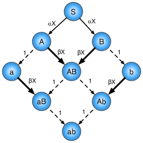
As in Chen et al. (2013) we shall only consider the case of two diseases and . We will always denote by capital letters () agents who actually have the respective disease, and by lower-case letters () those who had it in the past. Thus each agent can be in one of nine states: 0 (all susceptible), (infected with disease but not yet infected with , (infected with both), up to (immune to both). We assume that the dynamics is described by a set of nine rate equations
| (1) |
where is the fraction of the population in state , and where and are recovery and infection rates. We assume neither invasion nor birth or death, thus the total population size is fixed.
In the following we shall also consider only the restricted case of two symmetric diseases, where furthermore each agent has the same recovery rate and the same infectivity. In this case the model can be represented by the flow diagram shown in Fig. 1. In particular, the rate with which a susceptible agent acquires a disease is then proportional to the fraction of the population that carries this disease. In the following we shall denote this fraction by , where we have used the symmetry. In addition we denote by the fraction of susceptibles and by those who have or had been infected by one disease but not by the other. In terms of these three fractions, the original system of nine ODE’s can be reduced to three ODE’s,
| (2) |
Here, is the rate for a primary infection (i.e., for the infection of an agent in state 0), while is the rate for secondary infections, and the recovery rate was set to unity. Cooperativity implies that , i.e. .
These equations can then be either integrated numerically or discussed analytically. The former gives rise to plots like the one in Fig. 2, which suggests that there are discontinuous jumps when , where both and depend on the fraction of initially infected agents. The analytic treatment given in Chen et al. (2013) leads to exact inequalities which show that this interpretation is indeed correct, and that the jumps in Fig. 2 are not numerical artifacts.
An important observation is, however, that first order transitions are seen in the direct integration only when , the initial fraction of infected agents, is not zero. In the limit the fraction of affected agents stays always infinitesimal when is below or infinitesimally close to 1 (the threshold for a single disease outbreak), and cooperativity cannot become effective as long as is finite.
III Agent based stochastic models
In our simulations we assume that agents occupy the nodes of a network. They don’t move, i.e. we can attribute the nine states , and directly to the nodes. Time is discrete, with every sick node staying sick and infective for exactly one time step. Initially, all sites are susceptible (state 0), except for the set of seeds, which are nodes in one of the states or . We never allow any immune node ( or ) in the initial state. Unless specified differently, we assume that all seed nodes are doubly infected (i.e., ).
In principle we could allow both diseases to use different sets of links for their propagation. This would correspond to multiplex networks Gómez et al. (2013). We shall discuss this possibility later, but in most of the simulations (unless specified differently) both diseases use the same set of links.
The simulations use two data structures: First of all, we store in a character array of size ( is the number of nodes) the state of every node. This array will be updated in each time step. Secondly, we keep lists of “active” sites, i.e. of sites in one of the infective states and . From these lists we can see which nodes can be infected in the next time step and by which disease(s). Actually, we keep two such lists: One for the sites which are presently active, and one for those which will become active in the next time step. At the end of time step, the first is replaced by the second.
When implementing this, we have several detailed options, of which we considered two:
-
•
In the first we assume a latency of exactly one time step. Thus every newly infected node will not be active (i.e., infective) until the next time step. Notice that this concerns only newly acquired diseases. If a node newly infected with disease , say, had already disease , the latter is not affected. We call this also “parallel update with delay” or “SU” (for “synchronous updating”).
-
•
Alternatively, we can assume that a newly infected site becomes immediately infective. Thus, while we work our way through the lists of active sites, we immediately update their disease status. If done without precautions, this could introduce a dependency on the (arbitrarily but not randomly) chosen way how we go through the lists, and it could break the symmetry, if one type of infection is always done before the other. To avoid such artifacts, we shuffle the lists randomly in each time step, and we chose for each doubly infective active site at random whether it first infects with or with . We call this also “random sequential update without delay” or “AU” (for “asynchronous updating”).
Notice that any finite latency period is not supposed to change the universality class of any epidemic model (it would only change if latencies can become large, so that a new large time scale is introduced). But we should expect that it affects non-universal properties such as the precise locations of phase transition points. It seems that the difference between the two models is for some network topologies sufficient to shift a first order transition outside the range allowed by the physical values of the control parameters.
The two control parameters in our models are:
-
•
, the probability with which an active site infects a fully immune neighbor (i.e. a neighbor in state 0), and
-
•
which is the infection probability for a neighbor who has already (either in the present time step or in the past) acquired the other disease.
We could of course also differentiate between the latter two possibilities, but we did not in order to keep the model(s) simple. As we shall see, even with only two different infection probabilities there is a rich zoo of behaviors. Cooperativity corresponds obviously to the case . The opposite case will not be considered in the present paper.
For moderately large networks we let the epidemic proceed until all activity has died out, and measure then the properties of the clusters of immunes or . In addition we also performed simulations on very large networks where this would not be feasible. This concerns mostly regular lattices, where we used up to nodes. In these cases we stopped the epidemic before it could reach the boundary (or, if periodic or helical boundary conditions were used, before it could wrap around the torus). In this way we can effectively simulate the finite time behavior on infinite lattices, and could compare the growth of the set of active sites with the growth known for ordinary percolation Marro and Dickman (2005); Hinrichsen (2000); Grassberger (1983).
In the following sections we shall only discuss cases with perfect symmetry between the two diseases, where also both diseases use the same set of links. This is of course not very realistic, as many diseases have their own way of spreading. Alternatively we could consider multiplex networks (see Sec. VII), where each disease has its own set of links which is independent of the links used by the other disease. The fact that this can lead to completely different behavior is best illustrated by Erdős-Rényi (ER) networks. As far as single disease are concerned, the spreading on ER networks is of mean field type Bollobás (2001); Newman et al. (2001); Newman (2002). The same is true for multiple diseases, if their link sets are independent. Consider a doubly infected node on an ER network with finite mean degree . If this node is infecting neighbors with probability , then the chance for one of these neighbors to become doubly infected will be finite if the same links are used by both networks, while it will be for multiplex networks. Thus a double epidemic can spread even from a single infected seed if the same links are used, in contrast to the mean field behavior discussed in Sec. II. Ultimately, this is the basis for the intricacies found in the next section.
IV Trees and Erdős-Rényi Networks
Erdős-Rényi networks are random networks of nodes where any pair of nodes is linked with probability , with being the average degree of the nodes. In the interesting case of finite and large the networks are sparse, and thus there are no small loops. More precisely, the chance that a randomly picked node is on a loop of finite length tends to zero , when Bollobás (2001). Thus ER networks are locally tree-like. As a consequence, critical phenomena in spin models on trees and on ER networks are usually in the same (mean-field) universality class. For percolation, the situation is a bit more complicated, since on trees there exists an entire critical phase with two critical end points Hasegawa et al. (2014). Yet the situation is similar for trees and for ER models, since the classical Flory theory based on Cayley trees Stauffer and Aharony (1994) yields for the lower end point (where infinite clusters first arise) the same mean field critical exponents as theories based on ER networks Bollobás (2001); Newman et al. (2001); Newman (2002). As we shall see, this is dramatically different for cooperative coinfections.
IV.1 Trees, single node seeds
The situation is most simple for epidemics starting from one doubly infected node on a tree, with all other nodes being in state 0. Due to the absence of loops and because the epidemic can only spread away from the seed (all nodes on the backward path are immune), the spreading of coinfections is qualitatively always the same as for the spreading of a single disease. More precisely, in the case of a common network for and the threshold for either disease to spread is precisely at Newman (2002) 111In order to avoid confusion, we should point out that even above this value the average fraction of immune sites (the average order parameter) is still zero, and becomes non-zero only for Hasegawa et al. (2014). In spite of this, is often called the threshold Stauffer and Aharony (1994). for both models (with and without latency). For the model with latency the threshold for both diseases to spread together (i.e. for having a large cluster of doubly infected nodes) is (independent of ), while it is for the model without latency. For two independent multiplex networks, the latter two thresholds are replaced by , i.e. if there are no strong hubs the coinfection can survive only when . In all these cases the transition is continuous, i.e. second order.
Thus trees are trivial from this point of view, but there is still one interesting aspect. The spreading of epidemics on trees is mathematically described by a branching process Athreya et al. (1972). In a standard critical branching process, the survival probability decays as , while the average number of off-springs at time is constant. Finally, if the control parameter is a distance above the critical point, . All these apply to the model with latency (for any ), and to the model without latency if . But the case in the model without latency is different, as it corresponds to a doubly critical process, if .
To see this, it is useful to reduce the possible node states to three: uninfected (index 0), singly infected (“”) and doubly infected (“”). The model without latency is then described by the following transitions:
| (3) |
| (4) |
| (5) |
These are the possible transitions and their rates along any link from a mother to a daughter node. Such branching processes with two types of particles, where one type can only reproduce itself while the other can reproduce and produce particles of the first type, have been studied previously as models for cancer growth, where is a malign cell and is benign Antal and Krapivsky (2011).
Since there are in average links from mother to daughter, an node has in average descendents of its own type, while a node reproduces itself times. Thus, processes starting with one singly infected node are critical when , while processes stating with one doubly infected node are critical when . Since , in the latter case also the spreading of nodes is critical. The average numbers and are easily seen to satisfy
| (6) |
with . If we start with a node and take and (i.e., when ) we have then and . Thus, although the process is critical, is not constant but increases linearly with time. This also modifies the extinction probability. Using the standard generating function trick Athreya et al. (1972), one finds that the probability for to die out in a process that starts with a is
| (7) |
at the critical point, while it is
| (8) |
when and Antal and Krapivsky (2011). As we shall see, this difference between and has also consequences for ER networks.
IV.2 ER networks, single node seeds
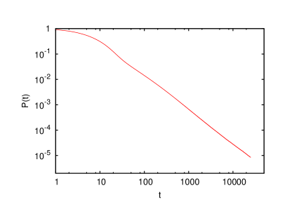
This is not at all the case for ER networks. In that case studying the time course of the disease is not very illuminating, as it follows the one for trees up to times when loops become important, and after that the behavior is rather complicated and does not scale. More interesting is to study the order parameter, i.e. the fraction of doubly immune nodes after the epidemic has died.
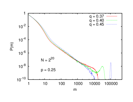
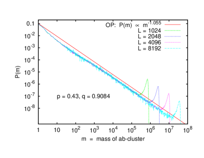
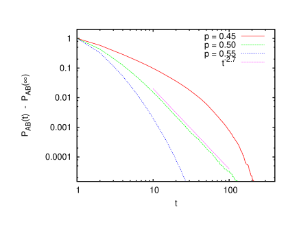
Throughout this subsection we shall use . In Fig. 3 we show distributions of the masses of the final -cluster, averaged over a large number of runs on the giant connected component. Here the model without latency was used, but the results for the parallel update with delay are qualitatively the same. For each we first generated a random network by randomly placing links and identified the giant component. Since this would give double links, we then rewired Maslov and Sneppen (2002) the links sufficiently often to eliminate all such double links. Then we run epidemics from randomly chosen seeds, rewiring times after every run. Since this alone would give a frozen degree distribution (rewiring does not change the degree distribution), we repeated this entire procedure until we had starts for each .
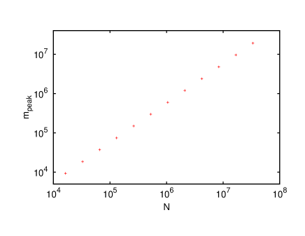
The data shown in Fig. 3 are for and . For these values the single disease dynamics would be critical, and indeed the mass distributions for the clusters of singly immune sites show the power laws with known from ordinary percolation Stauffer and Aharony (1994), with additional peaks at the high mass end due to events where there were also giant coinfection clusters (data not shown).
For small the distributions shown in Fig. 3 have the same power law, but this power law breaks down for . After a region without clear scaling properties there is a wide gap where , and finally there is a huge narrow peak for very large . A more careful inspection (see Fig. 4) shows that these peaks occur at , i. e. they are due to events where the -cluster contained a finite fraction of nodes. This is in striking contrast to critical OP, where the percolating cluster contains a vanishing fraction of nodes at the critical point.
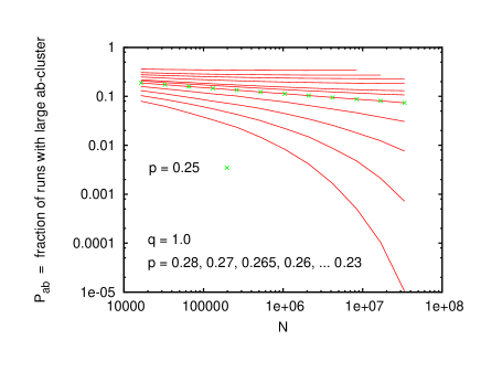
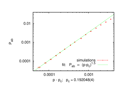
One might suspect that this doubly-peaked shape of the mass distribution results simply from the fact that the data shown in Fig. 3 correspond already to the supercritical regime. That this is not so (at least not in a naive sense!) is seen from Fig. 5. There we plot the fraction of runs that lead to a giant -cluster, where “giant” -clusters are very clearly defined by the very broad valley separating the peak from the left hand part of the mass distribution 222In a straightforward implementation most CPU time would be spent in following the evolution of giant -clusters to the very end. This is not needed, if one is interested only in the values of . Thus in obtaining the data for Figs. 3, 6, and 8 we interrupted the evolution when the size of the -cluster was above a threshold which had been determined before in runs with lower statistics. This introduces a negligible bias, but without this trick it would have been impossible to obtain this high statistics.. This fraction is plotted against for several values of near , and with in all cases. We see that decays fast with for all , while it approaches finite values for all . At it seems to obey a power law
| (9) |
with .
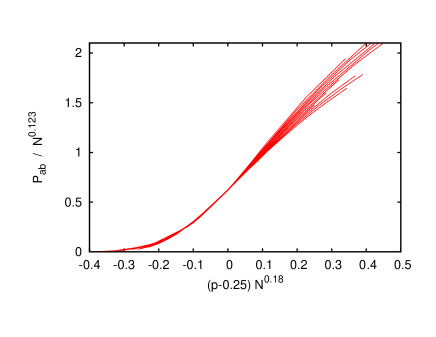
The data shown in Fig. 5 can be made to collapse reasonably well by plotting against (see Fig. 6, which suggests a finite size scaling (FSS) ansatz
| (10) |
with and .
For we also estimated the probabilities that there exists a giant single disease cluster, without a large cluster of the other disease. For OP, the chance to hit a giant cluster on an ER network of size decreases as Bollobás (2001). Our data (for ) are not very precise, since giant single disease clusters are not cleanly separated from small clusters (in contrast to Fig. 3), but our best estimate is , i.e. roughly the same decay as for giant -clusters. Thus disease , even if it finally dies out, has a positive effect on the survival of disease , since it makes the -cluster grow faster during early times.
All this indicates that is also the critical point for coinfections, and that shows qualitatively the same scaling (although with different exponents) as the probability for a random seed in OP to grow into the infinite incipient cluster. Indeed, for and , the latter is given for OP by , which is in that case also the scaling of the probability with which an infinite incipient cluster infects a random node. Since OP is a purely geometric problem, both are simply related to the density of the infinite cluster. This is no longer true in the present case. As we have seen, the density of the infinite -cluster is independent of , so that the order parameter exponent measured via its density is . Models were the density of an infinite cluster and the chance to generate this cluster scale with different powers and are well known Mendes et al. (1994); Janssen et al. (2004); Grassberger (2006), but usually and are both non-zero. The novel feature here is that one of them vanishes. Thus, while the transition looks like second order from the point of view of cluster growth dynamics, it looks like first order from the point of view of cluster geometry. This is a striking case of a hybrid transition Dorogovtsev et al. (2008); Goltsev et al. (2006).
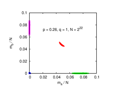
Finally, we should point out that mass distributions for clusters of singly infected nodes have in general two peaks at high masses (i.e. three peaks altogether). One of these peaks is due to events where only one of the diseases survives, while the other is from events where both diseases survive. This is even more clearly seen when looking at joint distributions of and , as shown for one particular set of control parameters in Fig. 7. There we see clearly four components: (1) without any giant outbreak, (2) with only an -outbreak, (3) with a -outbreak, and (4) with both outbreaks. The fourth component is also characterized by giant -outbreaks, while is small in the first three components. When is close to , single disease clusters are larger in the components (2,3) without giant -outbreaks than in component (4). This is reversed for large , where most nodes get both diseases, if there is a giant -outbreak.
For results are similar, as long as , where the value of depends on the detailed model. For random sequential update without delay, (more precise estimates will be given later). In this regime there exist still large -clusters containing non-vanishing fractions of all nodes. The behavior of is still similar to Fig. 5, but attempted data collapses as in Fig. 6 are even less perfect. Indeed, as shown in Fig. 8, there is a cross-over from for to for . The latter is the power law expected for two independent critical diseases spreading on ER networks Bollobás (2001). Also the dependence of on for and is as expected for two independent diseases Bollobás (2001), . The fact that there are different power laws for and are directly related to the discussion for trees in the previous subsection.
Thus, as far as the probabilities to lead to giant clusters is concerned, two cooperating diseases with are essentially independent. This is not true for the sizes of the giant clusters, where we find results similar to those shown in Fig. 7. In particular, whenever both single diseases have giant outbreaks, there is also a giant cluster of -nodes. The probability that there are two coexisting giant single disease clusters without large overlap is zero. This difference is easily explained by the fact that the decisions whether there are giant outbreaks or not are made at early times, when the networks still look tree like. The structures of the giant clusters are, however, decided at late times when (large) loops are abundant.
As is approached from above (keeping ), the double-peak structure of the mass distribution becomes more shallow (see Fig. 9), until it disappears when , and has a single maximum for . Thus is a (multi-)critical point.
IV.3 ER networks, multiple node seeds
The data shown in the previous subsection suggest that there exists already the possibility for having a giant -cluster even for , but that this cluster just cannot be infected by a single node seed. This would also be suggested by the analogy with the mean field model, where multiple seeds are needed to see the full phase structure.
Indeed, if we use a value of slightly below and start with a “seed” of randomly located doubly infected nodes, we find qualitatively similar behavior to that seen in Fig. 3, but with a much higher peak on the right hand side. Unless one goes to and to very large , this peak is still well separated from the rest of the distribution, and its position is essentially independent of (see Fig. 10 – for larger even less dependence on is found). Notice that we did not check that -clusters whose masses are shown in Fig. 10 are connected. But the very weak dependence on proves that they are, up to very small disconnected components.

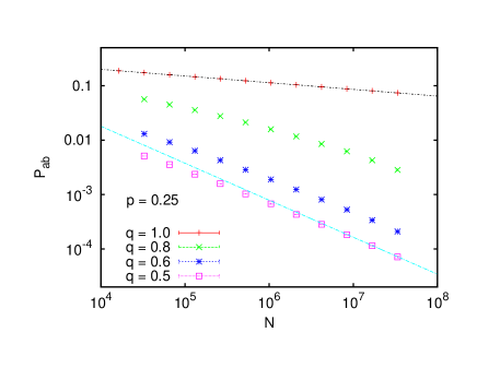
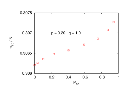
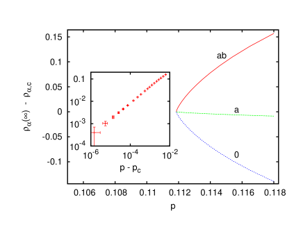
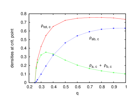
In mean field theory Chen et al. (2013), it was found that the seed had to contain a finite fraction of all nodes, in order to obtain a first order transition. To check whether this is also true on ER graphs, we plotted in Fig. 11 versus seed size , for and for one particular value of . We see that indeed the curves become steeper with increasing , and that they all cross an one particular seed density . Plotting these data against gives a very good data collapse if , as shown in the insert in Fig. 11.
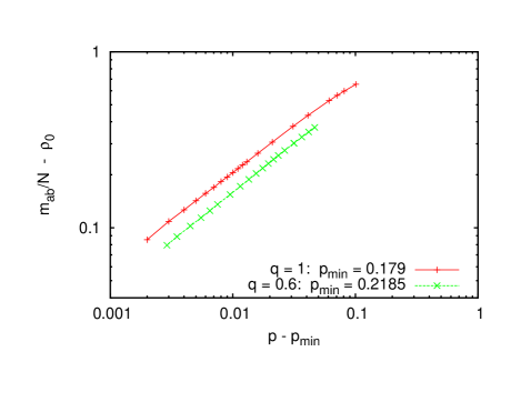
The (average) masses of giant -clusters does depend strongly on . Results for and for are shown in Fig. 12, where was chosen for each such that the right hand peak contained roughly between 1 and 10 per cent of all events. Within this range and for the values of () used in these simulations, the peak positions were stable within statistical fluctuations, at least for the values of shown. Figure 12 suggests that the fraction of the nodes in the next -cluster becomes equal to the fraction of initially infected nodes at some value , which is about 0.179 for and 0.2185 for . The value of increases with decreasing , until is reached for . For close to , the relative giant -masses satisfy (after subtraction of the seed density) a power law. The observed power depends slightly on , but this could be a systematic error, in which case the common power for both values of is .
For , the peak becomes wide and the valley separating it from the rest of the distribution becomes narrow and shallow, until finally for the entire mass distribution is single humped. Thus it seems that is a further critical point, where the coinfection cluster looses its identity. Qualitatively, it resembles the point in Fig. 2.
IV.4 Trees, multiple node seeds
With the hindsight obtained from studying ER networks, we can go back to trees and look whether we find there first order transitions, if we use multiple node seeds. For ER networks, first order transitions were always related to the existence of large loops. Since these loops are absent on trees, we expect that we will not find any sign of first order transitions, even if we consider multiple node seeds. As we shall see, this is verified by our simulations.
We studied Cayley trees with degree =3 for all central (non-leaf) nodes. On such trees the critical value for single diseases, above which an infinite cluster can exits, is . Notice, however, that even for all epidemics hit only a vanishing fraction of nodes in the limit , as long as .
As in the case of ER networks, we started with doubly infected nodes randomly located on the network (results are qualitatively the same, if we favor or disfavor leaves at this stage). For any , the distribution of -masses was always found to be unimodal. Thus, if we look for non-trivial results, we have to consider .
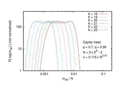
Indeed, we find bimodal distributions of -masses for , if we choose properly. Results for and and for the algorithm without latency are shown in Fig. 13 (for the algorithm with latency, results are quantitatively different, but qualitatively the same). In this figure, each curve corresponds to one value of . The number of seed nodes was chosen for each that both maxima have the same height, which gives within the statistical errors. If the observed double peak distribution were to indicate a first order transition, their positions should tend to constant densities when . Instead we see, however, that both peaks shift to the left as increases. Indeed, there is a decent data collapse if we plot against with , just as we would expect for a critical phenomenon. Also, the scaling of seed sizes used in Fig. 13 indicates a standard critical phenomenon. Finally, if we use smaller seed sizes, not only the height but also the position of the right hand peak decreases significantly, suggesting that the “giant” -cluster is not really well defined and connected, as it was for ER graphs.
We also looked at different observables, and they all confirmed our conclusion that there are no first order (or hybrid) transitions on trees.
V Regular lattices
On regular lattices, one can either study the properties of the giant -cluster after the epidemics have dies out, or one can follow the spreading as it evolves in time. Both strategies have advantages and disadvantages. In the former case it becomes infeasible to use too large lattices, whence one has to be careful about finite size corrections. In the latter one can stop the evolution before the finiteness of the lattice is seen, in which case there are no finite size corrections at all. But there are then finite time corrections. Fortunately, only a small fraction of the entire lattice is touched. This allows – eventually together with hashing Grassberger (2003) which we did not use, however, in the present work – the use of extremely large lattices, for which the finite time corrections can be made small as well.
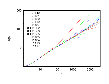
In time dependent simulations, the “classic” observables Grassberger (1983, 2003) are the average number of infectious at time , the probability that there exists still at least one infectious site, and , the r.m.s. distance of the infectious sites from the seed. In the following we shall not only consider seeds consisting of a single site, but also the spreading from an entire hyperplane. This gives much more precise results in cases with first order transitions, since it avoids the bottleneck in the nucleation phase that occurs in starts from a single seed. It also is more natural in such cases, since the growth of the infected cluster is then related to the growth of a rough interface that gets pinned at the critical point. Finally, we shall also measure various quantities related to the fact that we now have two agents and . This includes , the number of doubly infected sites, and , the average time lag between first and secondary infection for sites that finally get both diseases (the precise definition is given later).
A crucial difference between sparse random networks (like, e.g., ER networks) and regular lattices is that the latter contain small loops. Due to the absence of small loops on ER networks, the critical point for spreading from a single node seed was the same as for single diseases, . Thus the cooperativity did not lead to a renormalization of the threshold, unless multiple seeds were used. This is not so for any finite dimensional lattice. Assume that is slightly below the critical value for single diseases. Then there is a finite chance that both diseases survive for a short time . During this time, they will help each other and thus their chance of further survival is enhanced. In other words, for each disease the presence of the other disease renormalizes the growth rate.

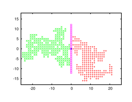
As an illustration, we show in Fig. 14 the final configuration on a square lattice with nearest neighbor contacts. On this lattice, the threshold for a single disease is at Stauffer and Aharony (1994). For coinfections with the parameters used in Fig. 14 it is at . The reason for this shift is easily seen from the structure of the cluster. It consists of a “backbone” of doubly infected sites, surrounded by two “halos” with single infections. The latter have a finite thickness, of order , where is the correlation length exponent. Therefore, there is always a site with disease close to any site with disease and vice versa. Thus cooperativity is always at work.
Notice that this argument would break down at , where giant clusters of single diseases exist. Below , outbreaks can only be small for both diseases or large for both. In the following, we will restrict our attention to .
V.1 Two-dimensional lattices, short range infections

Mass distributions of -clusters obtained at the critical point for a randomly chosen large value of are shown in Fig. 15. The upper panel shows that the bulk of the data show the well known scaling of OP Stauffer and Aharony (1994), while the lower panel shows that the right hand peaks correspond to giant clusters whose masses scale exactly as , where is fractal dimension for OP. These data not only show that there is no first order transition, but they suggest also strongly that the critical point is in the OP universality class. We should add that similar data were obtained for other values of (including ) and for the algorithm with delay.
Values of for near the critical point for are shown in Fig. 16. More precisely, for easier comparison with OP we plotted there versus , where is the value for percolation in 2 dimension Grassberger (1992a). Lattice sizes were so large that the cluster never touched the boundary, and the algorithm with latency was used. We find of course important finite time corrections, but the results for are fully compatible with the expected asymptotic scaling. We should add that this value of is also compatible with the estimate obtained from mass distributions.
This absence of a first order transition and universality with OP was confirmed for the algorithm without latency, for other values of , and for the square lattice with next-nearest and also with next-next-nearest neighbors (i.e. with 8 resp. 12 neighbors). In all cases it was verified that for large .
There are, however, two novel scaling laws for in the vicinity of the single disease critical point . Both can be most easily understood by referring to Fig. 14. As we said, the thickness of the “halos” of singly infected sites around the doubly infected backbone is equal to the correlation length of OP. When , this correlation length diverges.
Consider now the limit where there is no cooperativity. In this limit also , and increasingly larger portions of the total cluster are made up by singly infected sites. This means however that also cooperativity should become less and less effective in this limit, implying that . This is indeed verified in Fig. 17. As seen from the insert in this figure, a decent fit is obtained by the power law with a new independent exponent
| (11) |
For the other scaling law, consider an arbitrary value . For any there will be a non-zero chance of survival, i.e. for . Due to universality with OP we expect that this asymptotic value is reached faster that with a power law,
| (12) |
for any exponent (as was also verified numerically for , see Fig. 18). Consider now the case , where there is also a non-zero chance that single infected clusters survive forever (if the other disease had died out earlier). Exactly at the probability that only one of the diseases, say , survives should decay as with known from OP. Moreover, there will be a small chance that survives for some time by spreading into one direction, and survives by spreading into the opposite direction. Such an epidemic would look superficially like an epidemic of double infection, but since there is no cooperativity (since both diseases survive in different regions), it has a much higher chance to die. Let us define as the probability that both diseases have not yet died out at time . In Fig. 18 we show a log-log plot of versus . The data clearly suggest a power law
| (13) |
with exponent .
A simple upper bound on this exponent is obtained as follows. We first define a boundary as “killing”, if any epidemic that tries to infect a site on it is killed. Such a boundary has a much stronger effect on clusters than normal boundaries, where only the branch that would pass through the boundary is deleted. Clusters which start on a killing boundary have therefore a much smaller chance to survive. Numerically, we found by simulations that with . Consider now the situation shown in Fig. 19, where two OP clusters start from the same site on a killing wall, and are forced to grow into opposite directions. Any such configuration would contribute to , which gives immediately
| (14) |
In this paper we always decide “on the fly” whether a site or node can be infected. But we could also have decided this before the simulation, since any node can be infected at most once by either one of the two diseases. The results would be identical. In the latter case we are dealing with frozen randomness. There is a rather general theorem Aizenman and Wehr (1989); Cardy (1999) that forbids first order transitions in two-dimensional systems with quenched randomness. Although it is not clear whether this theorem applies strictly spoken to the present model, the general ideas should. It definitely applies to the cooperative percolation model of Janssen et al. (2004); Bizhani et al. (2012) and to the zero- random field Ising model, since these can be mapped onto the Potts model, and it explains why in this case critical pinning is in the OP universality class Drossel and Dahmen (1998); Bizhani et al. (2012)). It strongly suggests that there exists only one universality class of critically pinned interfaces in isotropic 2-dimensional media, namely that of ordinary percolation.
V.2 Four dimensions and above
V.2.1 , Point seeds
The results of the last subsection might suggest that in general, there are no first order transitions on regular lattices. To show that this would be wrong, we present simulations for the simple hypercubic lattice with , as a typical high dimensional lattice. Lattice sizes are in each case sufficiently large that we have no finite-size corrections at all.
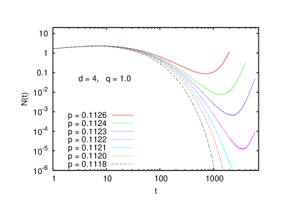
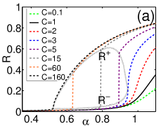
Panel (a) shows results for . The best estimate for from these data is , but a more precise estimate will be given later.
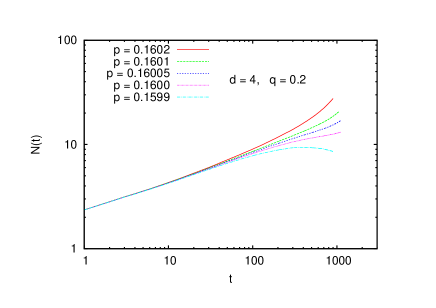
Panel (b) is for . Here cooperativity is much weaker, and thus our estimate is much closer to the value for OP. Superficially, this plot might suggest a power law and thus a second order transition, but all structures seen in this plot are real (statistical errors are much smaller than the line thicknesses) and suggest also a (weak) first order transition.
In Fig. 20 we show results for , for two rather extreme values of and for several . For the transition is obviously first order. For the epidemic seems first to die out (faster than with a power law!), but finally – if it turns around and increases with a power much large than that for critical OP. This is very reminiscent of nucleation where clusters have to become large before they can grow further with high probability. As long as the cluster size is small, it is much more likely that the cluster dies than that it grows. For (which is only very little above the OP value Grassberger (2003)) the situation seems to be different. At a rough glance, the data suggest a power law for , which then would suggest a second order transition. But actually none of the curves in Fig. 20b is asymptotically straight (all structures seen in this plot are real, since stochastic errors are much smaller than the line thicknesses), and a closer look shows that also now curves bend down and pass through a (much less pronounced) nucleation phase.
In the next subsection we will present more clear numerical evidence for the absence of a tricritical point and for the transition being discontinuous for all . In the following we will give more heuristic arguments, supported by indirect numerical evidence.
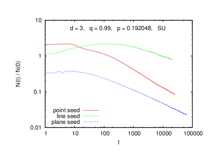
To understand the mechanism behind this scenario, it is helpful to look at , the number of doubly infected sites. This is shown in Fig. 21 for and for four values of . More precisely, we show there , i.e. the probability that an infected site is doubly infected. This at first decreases steeply for all four values of . It is only in the supercritical case that this decrease stops and finally even turns around. This suggests that at first and were spreading into different directions, with little overlap between them. This little overlap is not enough to generate enough cooperativity which would prevent them from spreading further apart – and dying finally because is subcritical for single epidemics and because two infinite clusters cannot coexist anyhow. It is only for and for large that occasionally two clusters with sufficient overlap developed so that they continue to spread coherently. Notice that this did not happen in , since there it is extremely unlikely that two clusters can grow without having much overlap.


(b) Part of the same data, bu shown as against , with . Since the data for small have obviously large non-scaling corrections, only data for are plotted.
In the next subsection we will see that can be estimated much more precisely by using infected hyperplanes as seeds rather than single points. In this way we will find for . Using this value, we plot in Fig. 22 how , the probability that a single infected site creates an infinite epidemic, depends on . We see that the curve becomes steeper and steeper on a log-log plot as , indicating that has at threshold an essential singularity. This reminiscent of nucleation phenomena where the chance for small droplets to become macroscopic in metastable phases behave similarly Debenedetti (1996). As we shall see in the next section, the behavior in three dimensions is very different.
V.2.2 Hyperplane seeds
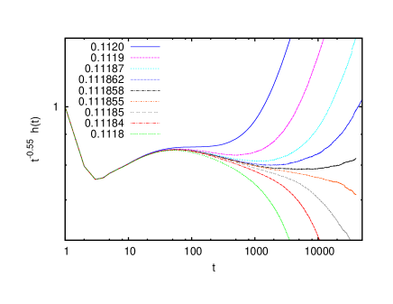
In order to avoid the nucleation phase (which, among others, prevents a precise estimate of ), we also made simulations where we started with an entire infected hyperplane as seed. In this case the boundary between healthy and sick regions is formed by a propagating interface which starts off flat and becomes increasingly rough. For the growth finally stops and the interface gets pinned, while it continues to move forever for . Exactly at , one might expect it to be in the universality class of critically pinned interfaces in isotropic random media Family and Vicsek (1991); Barabási and Stanley (1995); Bizhani et al. (2012, 2014). In Fig. 23a we show versus for and several values of close to . All data in this plot were obtained from lattices of size with laterally periodic (more precisely, helical) boundary conditions. The diseases started at the base surface and was so large that the upper boundary at was never reached. The base surface had size with between 256 and 512. This is big enough so that finite size corrections are small (for a more detailed discussion see below). We see that there is a clear power law
| (15) |
when , which is therefore our best estimate of .
To demonstrate the quality of the data on the one hand and the fact that this power law has important corrections on the other hand, we show in Fig. 23b the same data plotted as against . Notice the much enlarged resolution on the -axis. We see that there is actually no single curve which is clearly a horizontal straight line. The error bars on and are a naive attempt to take into account this uncertainty.
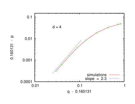
The most dramatic result from this plot is the vastly improved estimate of . It agrees with the previous estimate from point seeds, but it is about four orders of magnitude more precise. Similar plots were also produced for other values of in the range . They are all qualitatively similar, and they suggest that indeed the percolation transition is discontinuous in this entire range (estimates in the range were inconclusive). The results for are shown in Fig. 24. They suggest a power law . Notice that this is in contrast to the case with cooperativity between different neighbors Dodds and Watts (2004); Janssen et al. (2004); Bizhani et al. (2012). In that case, there exists a tricritical point such that the transition id continuous for and discontinuous for . The absence of such a tricritical point in the present model might be related to the appearance of a new divergent length scale when , as discussed in connection with Fig. 14.
Approximately, the data shown in Fig. 23 obey a finite time scaling (FTS) ansatz
| (16) |
with . Similar ansatzes describe also reasonably well all data for . We believe that this actually would describe the asymptotic behavior, and that the estimate of is correct up to about 5 percent. But the fit is far from perfect and – what is much worse – if no corrections to scaling were applied, similar FTS ansatzes for the data obtained at different values of yield substantially different critical exponents. This is e.g. seen by plotting on the same log-log plot values of versus for different values of , choosing for each that value of where the curve is straightest. Such a plot is shown in Fig. 25. We see that actually none of the curves is straight, their average slope decreases , and they all seem to become parallel to the curve for (which is the least curved one) for very large . For small the slope becomes steeper with decreasing , in agreement with our claim that we see a very slow cross-over from OP. The latter would correspond to , and the exponent there is Grassberger (1986).
A similar FTS ansatz holds also for the height of the interface. There are several ways to define this hight. The data shown in Fig. 26 use just the average value of the coordinates of the presently infected (“active”) sites, . They can be fitted by the ansatz
| (17) |
with . Again this is far from perfect, as can be seen from a similar blow-up as for the densities, see Fig. 26b.
Scaling laws like Eqs. (16,17) apply also to ordinary percolation Grassberger (1983), where the exponents are however different. In the present case the cluster behind the growing surface is compact, i.e. its height grows proportionally to its mass. The latter is given by , from which we obtain
| (18) |
which was indeed imposed as a constraint on the values used in Figs. 23b and 26b. For OP the cluster is fractal with dimension , so that at the critical point , leading to ). But things are not entirely clean. First of all, for no value of is a clean power law. Secondly, for the curves decrease both in Figs. 23b and 26b. This could mean that the densities of the grown cluster are not constant in this region, but we will show later that this is not the case. Most embarrassing is that the estimates for obtained from and from are slightly different. The difference is very small (it is within the error bars quoted above), but it is statistically significant. The nominal value of from is slightly higher than that obtained from . The only explanation for this are finite size corrections. Indeed, one expects finite size corrections to be positive for and negative for . This was also verified explicitly by making runs at smaller values of .
All this shows that: (i) Yes, there are clear indications for finite size corrections. But the very fact that they are seen and qualitatively as expected makes us sure that they are well under control; (ii) They cannot be responsible for the deviations from the expected FTS and for the observed -dependence of the critical exponents, which most likely are a very slow cross-over from OP. As a result, all estimates of critical exponents in this subsection have to be taken with some caution.

In the following figures we show several more observables, all of which show scaling laws and demonstrate thereby that the percolation transition is actually hybrid. They also show that at least the rough features of the scenario depicted so far are consistent.
(1) In Fig. 27 we show , the velocity by which the height grows for very large times, when . It is simply obtained from the straight lines in the upper right part of Fig. 26a. These data were obtained by using the fact that the (hyper-)surfaces for are rather smooth in . Thus the simulation box can be much wider than high. Moreover, we always checked that the height difference between the highest and lowest active site is . As long as this is guaranteed we can “recycle” the part of the simulation box below the lowest active site. That means we erase in this part the old configuration and overwrite it with the new growing part on top of the surface. Effectively, this means that we replace the simulation box by a torus, and let the surface circle around it. Two data sets, for and for are shown in Fig. 27. Also indicated in this figure are the results for OP and the predictions of the “standard” model for pinned rough interfaces, where overhangs are neglected Le Doussal et al. (2002); Tang (2009).
Both data sets are compatible with power laws with similar exponents. If we accept the FTS ansatz, we obtain indeed
| (19) |
This is indeed compatible with the data, although there are also important corrections to scaling. These corrections are larger for than for , in agreement with our previous discussion. Whatever the true exponent is, it seems very unlikely that the model is in the same universality class as the model without overhangs.
(2) The cluster below the growing surface is compact for , but it does contain holes. Thus the densities , and are all non-zero. Here, is the density of the cluster at height , after the interface either has stopped growing (for ) or has passed far beyond (for ). Results for are shown in Fig. 28 for . We see a clear distinction between sub- and supercritical values of . The density at is .
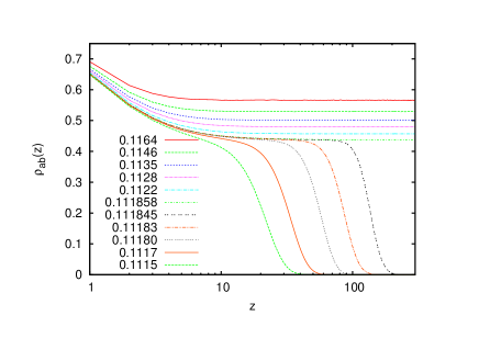
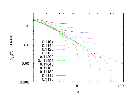
(3) Fig. 28 shows indeed several scaling laws. The most obvious maybe (but the least interesting, because this scaling is already inferred by the results given above) is how the pinning height scales with the distance from . More interesting for us now is the convergence to at small times seen in Fig. 28b. There the data of Fig. 28a are just re-plotted as against , instead of against . We see for a power law with exponent .
(4) In Fig. 29 we show the limiting densities and as functions of ( by symmetry). As seen from the inset, we have for the -density again a power law,
| (20) |
with . The same power law (with the same exponent) is also seen for . For the density of -sites, either the amplitude in this power law is very small or the exponent is zero.
(5) According to our scenario, the percolation transition is first order in , while it is continuous in , because there is a bottleneck similar to nucleation in the former that is absent in the latter. This bottleneck appears because the two diseases grow first into different directions in , which is much less likely in . Thus in the growth of the two diseases is more or less synchronized, while this is much less so in . Therefore we expect also the average time lag between first and second infection to be large for those sites which finally become doubly infected.

For all sites whose secondary infection happens at time , we denote as the average time lag between primary and secondary infection times and . Data for versus are shown in Fig. 30. We see indeed the expected behavior: While this quantity is finite in the supercritical phase (where both diseases propagate together), it increases very fast in the subcritical phase, while its growth is (very) roughly described by a power law at the critical point. For its asymptotic value seems to scale roughly as . But we should also point out that the interpretation of these data is far from trivial. First of all, increases also in at the critical point (although only logarithmically). And secondly, the increase in the supercritical region is at large faster than linear with , which cannot hold on forever, as is strictly less than .
(6) Finally we show in Fig. 31 fractions of infected (i.e. active) sites that are doubly infected, similar to the data shown in Fig. 21 for point seeds. We see a qualitatively similar behavior, except that now it is clear that tends at to a finite positive value (equal to ) when . This seems at first to be at odds with the fact that the average time lag between the two infections diverges in this limit, but it has an easy intuitive explanation: Assume that and start at some time from the same site. When they meet again at some other site, one of them (say ) will most likely arrive earlier then the other. So will find an easily infectable -cluster and it will run after . But whenever makes a detour instead of taking the shortest path, can also take the shortcut, and thus it will slowly catch up. Finally, there will be a small chance that arrives at some site simultaneously with , and the whole repeats.
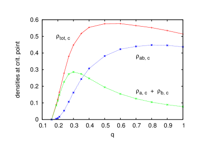
The single site seed simulations of the previous subsection have already suggested that the transition is discontinuous for all , and that there is no tricritical point. This claim can be made much more strong by using hyperplane seeds and estimating the threshold densities as in Figs. 28 to 29. Results obtained in this way are shown in Fig. 32. We see that all densities are indeed non-zero at threshold for all . They are very small for small (in particular, is tiny), but the data show clearly that there is no tricritical point.
V.2.3
We have not made simulations in . For we expect qualitatively the same result. There, the chance that and can spread for some finite time without interfering is even larger, but finally they should overlap, and then a compact cluster is formed. This is no longer true for , which is the upper critical dimension for OP. For multiple infinite clusters can coexist, and thus and can spread forever without cooperating. This might lead to a scenario with a tricritical point . For cooperativity would dominate, leading to . This would then prevent single diseases from spreading at , and one has a first order transition. For , in contrast, it would be entropically favorable for the epidemics to spread apart, leading to and second order transitions.
This seems to be at odds with the fact that there are first order transitions on random (ER) networks, but this is easily explained by the different limits taken in the two cases. On finite-dimensional lattices we always consider first the thermodynamic limit of infinite system size before we take the limit . On random graphs, in contrast, we take first the infinite time limit and let then the system size diverge. If we would also take the limit of infinite system size first for sparse random graphs, we would end up with trees for which there are indeed no first order transitions.
V.3 Three dimensions
We left the case to the end – not because it is the least interesting, but because it is the most puzzling. And we wanted first to be sure that we can numerically distinguish first and second order transitions, and that we understand the basic mechanisms behind them.
V.3.1 Point seeds
In Fig. 33a we show versus , for and the algorithm without delay. Seeds were single points. The solid straight line shows the scaling for OP Grassberger (1992b). Obviously this presents a perfect fit for . Thus we conclude that even with very strong cooperativity, the percolation transition is second order and in the OP universality class. The same conclusion was drawn from the survival probability and from runs starting with plane seeds (data not shown).
Panel (a): Data obtained by the algorithm without delay. The solid straight line represents the scaling for OP. Panel (b) shows data for the algorithm with delay.
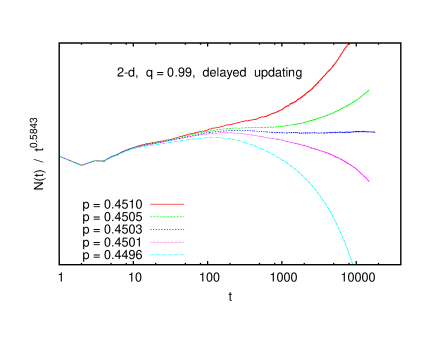
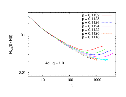
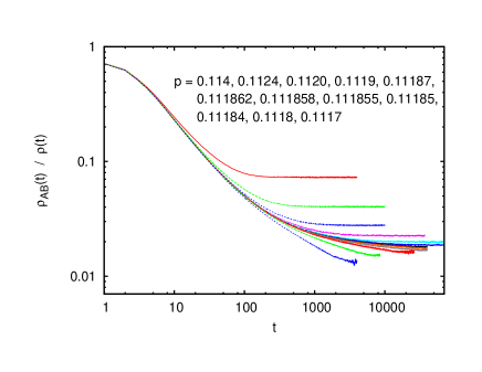
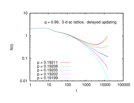
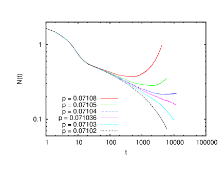
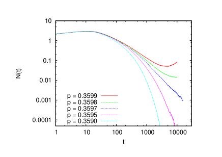
The situation is more complicated for the algorithm with delay. Data analogous to those in Fig. 33a are shown in Fig. 33b. Again the simple cubic lattice is used with point seeds. These data indicate clearly a first order transition at . The experience of the 4-d simulations might warn us that this is slightly overestimated, but at least a second order transition seem definitely ruled out.
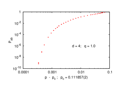
As for the case, we expect a better estimate for from seeds which form an entire plane of size . We will show such data later. But before that, we shall use the precise values obtained in that way for the entire range to estimate the critical densities. A plot analogous to Fig. 32 (which shows the data for ) is given in Fig. 34. Again we see clearly that there is no tricritical point, and the transition is discontinuous in the entire range .
Consider now the case where the seed consists not of one doubly infected site, but of two singly infected neighboring sites and . One of these sites has disease , and the other has disease . One should naively expect not much difference, but the data – shown in Fig. 35 – look completely different. There is no longer any indication of a first order transition. Rather, the data are again – as in the model without latency – perfectly in agreement with OP, as is also indicated by the same straight line as in Fig. 33a.
Before we go to explain this puzzling behavior, we show another puzzle in Fig. 36. There, again for epidemics starting from a single point simulated with delay are shown as in Fig. 33a, but in contrast now the lattice is not the simple cubic lattice with nearest neighbor contacts. Rather, each site can now infect 14 neighbors , where . The last 8 of these are neighbors in a body-centered (bcc) lattice, while the first six are next-nearest neighbor bonds on the bcc lattice. This time there is again no indication of a first order transition, and the data are again fully compatible with OP.
After these findings we went back to the algorithm without latency, to check whether similar complications arise also there. They don’t. In that case the transition is robustly of second order, independently of the seed and of the lattice type. Also, on the bcc lattice with next-nearest neighbor bonds the transition remains second order, if the two diseases start on neighboring points. On the other hand, on the sc lattice the transition seems always second order when the epidemics start from two sites with odd Manhattan distance, while it is first order whenever the distance is even.
Although this looks all very strange, an explanation is easy – although, as we shall see, it can only be part of the story. A first hint comes from the fact that the sc lattice is, in contrast to the bbc lattice with next-nearest neighbor bonds, bipartite. Therefore sites on the sc lattice can, like sites on a checker board, be colored black and white or odd & even. If the origin is even, then any path from the origin to any even site has an even length, while all paths to odd sites have odd lengths.
In the algorithm with delay, cooperativity is active only when both diseases try to infect a site at different times. When they arrive at the same time, then there is no cooperativity due to the latency. Consider now an even site , when the seed is the doubly infected origin. Then cooperativity is not effective, if both diseases reach along paths of equal lengths. If infections propagate largely along shortest paths, this then reduces cooperativity substantially. This should not be relevant for very late times, since then most paths will be longer than minimal ones. But it should be relevant at intermediate times, where it reduces the effective cooperativity. Thus spreading passes through a difficult intermediate “bottleneck” phase, resulting in a first order transition.
This argument obviously does not apply when the two diseases start at different points which are separated by an odd Manhattan distance (i.e., on sites of different parity). In that case they arrive at any site at different time anyhow, and the distinction between the two algorithms no longer plays a big role.
On non-bipartite lattices, finally, different paths between the same two points can have both even and odd lengths, and thus the diseases can arrive with any time lag. Now there is still a difference between the algorithms with and without delay, but it is much reduced when compared to bipartite lattices. Our finding that the transition is second order on the nnn bcc lattice is thus non-trivial (a priori, it could have been different), but not very surprising either.
While all this sounds convincing, we should warn the reader that things are actually no so clear. This is seen by replacing the sc lattice with nearest neighbor links by yet another lattice: The sc lattice where each site has 12 neighbors and , where . As the bcc lattice with additional next-nearest neighbors, this is not bipartite and thus according to our arguments this should have no “nucleation” phase and should show thus a second order transition in the OP universality class. But the data shown in Fig. 37 definitely do not show the latter. Rather they suggest a first order transition with a very weakly pronounced bottleneck (notice the different y-axis scales in Figs. 37 and 33b).
V.3.2 Plane seeds
For the algorithm without delay we verified that indeed the transition is continuous and in the OP universality class, as expected from the point seed simulations. We do not discuss this further, and consider only the algorithm with delay. We first discuss simulations on the sc lattice with nearest neighbors only.
If we start with an entire doubly infected plane as in subsection V.2.2, every point is connected to the seed by paths of even and odd length. By the above argument we expect that there will be a second order transition in this case. This was indeed verified (data not shown). In order to obtain a first order transition we must make sure that all paths from any seed site to a fixed target site have the same parity. This is the case if we color the base plane like a checkerboard and start with all black sites doubly infected, while all white sites are susceptible. When simulating this, we of course have to make sure that bipartivity is not broken by the lateral boundary conditions. This would be the case for naive helical b.c. (in which case we indeed observed a cross-over from one asymptotics to the other, when ). But bipartivity is conserved by helical b.c. in the horizontal plane, if we use an even number of sites (we used planes with sites, with ), but use as neighbors of site the sites and (both modulo ) with odd . More precisely, we used when is even, and the closest odd number to when is odd.

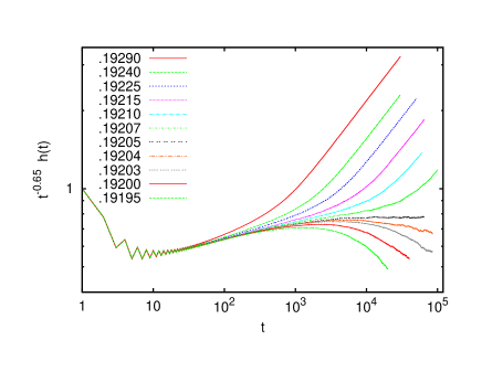
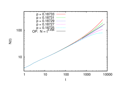
Data for and obtained in this way are shown in Fig. 38 In order to compare with the point seed simulations we used again . As in Figs. 23b and 26b we multiplied the data by suitable powers and to make the curves for (approximately) horizontal at large . The powers were again constraint to satisfy , as required by the compactness of the infected cluster. The chosen values are seen to give a decent fit, although it is – as in four dimensions – far from perfect. As in four dimensions, these simulations gave a much more precise estimate of than the point seed simulations. Our best estimate is .
As in , these data are compatible with the FTS ansatzes Eqs. 16 and 17, but we have not yet done a very detailed analysis and – what is even more important – we have not yet checked carefully that all values of give rise to transitions in the same universality class. Since surfaces near the pinning point are more rough in than in , also finite size corrections are more important for those sizes that are presently feasible. We hope to make a more complete analysis of the model in a future publication.
Here we add just a few more remarks:
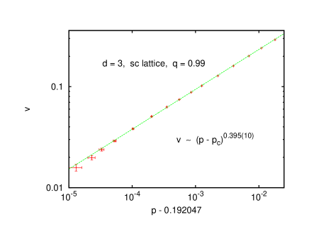
(1) We measured quite carefully the scaling of the interface velocity of the interface in the supercritical phase. It is again obtained by using the data in the upper right corners of Fig. 38b. Results are shown in Fig. 39, and show a very clean power law,
| (21) |
with . As in , this seems to rule out the possibility that our model is in the universality class of critically pinned rough interfaces with a single field and no overhangs Le Doussal et al. (2002); Tang (2009), where Nattermann et al. (1992); Leschhorn et al. (1997).
(2) We found again that seems to approach finite positive values in the supercritical phase and that these values scale with the distance from the critical point. In the subcritical phase (including the critical point itself) they diverge as .
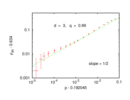
(3) After the infection has died out, the densities at given height show a behavior qualitatively similar to Figs. 28, although the data were much less clean due to the larger finite size corrections. In particular, due to huge corrections to scaling we were not able to give a precise estimate of the order parameter exponent defined in Eq. 20. We can only say for sure that it is (see Fig. 40).
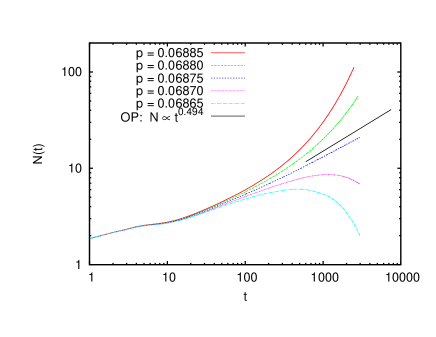
Finally, we made also simulations with an infected hyperplane for the last model discussed in the previous subsection, where the infection can pass to sites that are distances 1 and 2 away in the six coordinate directions. The precise threshold (for ) turned out to be , and . The latter is compatible with the value on the sc lattice, which suggests that both models might be in the same universality class in spite of the big differences between Figs. 33b and 37.
V.3.3 Further indications for hybridicity
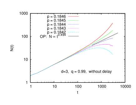
Although it should be clear by now that all “first order” transitions discussed in this paper are indeed hybrid, there is one aspect in which the 3-d model with delay is strikingly different from the situation in 4-d. For point seeds in , the behavior of , , and are all reminiscent of nucleation (for example, see Figs. 20a for and 22 for ; the behavior of is, near the transition point, very similar to that of and is not shown here). All these observables do not show power laws but rather exponentials or stretched exponentials (with our precision, we cannot distinguish between these).
For , in contrast, all three observables seem to show power laws. For and this is seen in Figs. 41 and 42. For we find (approximate) power laws not only for point seeds, but also for plane and line seeds, see Fig. 43. Although there are large corrections, all these are consistent with a power law with the same exponent, . Thus we do have a bottleneck in the spreading of coinfections on the sc lattice with the SU algorithm, but this bottleneck seems not to be associated with the essential sigularitites typically found in nucleation Debenedetti (1996). Very similar behavior will be seen in the next section.
VI Long range infections
While high dimensions provide the standard cross over from local to mean field behavior, another well known path is to go via long range interactions. In the present case of epidemics, this means long range infections.
Assume that agents are placed on the sites of a -dimensional regular lattice (in the present paper we shall only deal with ), and that the probability for an infected site to infect another site follows asymptotically a power law,
| (22) |
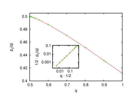
so that the probability to infect at least one site at a distance decays as . When is large, we recover the local model, while mean field behavior holds for . The border between these two regimes has been studied in detail for OP, with the most recent and detailed simulations reported in Grassberger (2013a, b). For critical 2-dimensional OP, mean field behavior (as far as critical exponents are concerned) holds for , while local OP behavior holds for . In between there is a region where the critical exponents depend on . Indeed, it is still an open question whether local OP behavior holds only down to or continues to hold down to Linder et al. (2008); Grassberger (2013b).
In view of the dramatic differences seen in three dimensions between the models with and without delay, we first made test runs with both schemes. We found the results again to be rather different (scaling sets in much earlier for the update without delay), but it seemed that the transitions were in both cases discontinuous for large . Thus there does not really seem to be as much a difference as in , and we did not study the model with delay any further.
In the following simulations we used the model without delay and the precise form of used in Linder et al. (2008); Grassberger (2013b). For each site we have three potential contacts distributed according to Eq. (22), and the diseases are transmitted through each contact with probability . Initial conditions were such that one site had disease , while one of its neighbors had disease . We used lattices with sites and helical b.c. (notice that we could have gone to much larger lattices by using hashing as in Grassberger (2013b), but we wanted to keep the codes simple).

Plots of versus for are shown in Figs. 44a (for ) and 44b (for ). In each plot results are shown for several values of close to . In both panels we see large corrections to scaling, but both are compatible with power laws
| (23) |
at the respective critical points. While for , as for ordinary percolation, this exponent is negative for , indicating a first order transition.
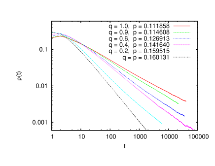
This suggests that there should be a tricritical point for some value of in between. In order to test this, we plot in Fig. 45 the estimated exponents against , together with the exponents for the single epidemics. As expected, the two curves are very close for large (i.e., for relatively short range contacts), since we have already seen that the coinfection transition is in the OP universality class when the contacts are short range. For we expect to diverge to , since in that limit we should obtain the result for random graphs. Our data are compatible with this.
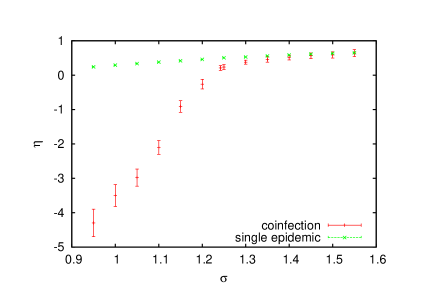
Our data are not precise enough to study the tricritical point in detail. It could coincide with the point where the two curves in Fig. 45 seem to separate 333Naive fits to the raw data would suggest that the two curves already separate already for . But one should bear in mind that there should be strong cross-over corrections near a tricritical point. Indeed, we found large finite- corrections for which suggest that our estimates of may be underestimated in this region.. Alternatively, we could assume that the transition becomes first order when , which would give . If the latter is to be identified with the tricritical point, then the two curves are presumably different for all in the plotted range, but the difference is extremely small for . In any case we should stress that Eq. (23) describes the data for all intermediate values of , including the point where . In contrast to typical tricritical phenomena in other systems, the scaling is not qualitatively different at the tricritical point. But we should warn the reader that we do see large scaling corrections (see footnote [61]), and as in the four-dimensional case (see Fig. 20b) and as in single-disease infection with long range Grassberger (2013b), this might indicate that the true asymptotic behavior is quite different.
We also made simulations for . We verified that OP is reached when becomes close to , and in each case the data were compatible with Eq.(23). For all the values of smoothly passed from positive to negative values when was increased.
VII Scale-free and small world networks
VII.1 Scale-free networks
Most real world networks have strong hubs and have heavy-tailed degree distribution. They are often modeled as scale-free, i.e. the degree distributions satisfy approximate power laws. The most popular model leading to scale-free networks is due to Barabási and Albert Barabási and Albert (1999) (BA). Therefore it is of practical importance to ask whether cooperative epidemics can show first order transition on it.
It is well known that the BA model leads to continuous percolation transitions in cases like interdependent networks Buldyrev et al. (2010); Baxter et al. (2012), networks with cooperative nodes Bizhani et al. (2012), core percolation Liu et al. (2012), or explosive percolation Achlioptas et al. (2009); Radicchi and Fortunato (2009). In all these cases other random networks either show first order transition or extremely sharp transitions which at least superficially look like first order. This strongly suggests that the percolation transition for cooperative coinfections is also continuous on the BA model.
Indeed, simulations showed no sign of any first order transition. This is also easily understood heuristically. For a first order transition one should have weak cooperativity at early times (e.g. because the network is tree-like), but high cooperativity due to many long loops at later times. In the BA model most loops are short, and due to the strong hubs there is no bottleneck in the growth that could lead to nucleation.
VII.2 Small world networks
Real-world networks not only have hubs, but they also show the “small-world effect” (nodes are connected by very short paths Milgram (1967), so that the diameter of the network increases or even slower), and they are strongly clustered. Such networks are called “small world networks”. The most popular model for small world networks is the Watts-Strogatz model Watts and Strogatz (1998).
In this model one starts with a regular lattice (typically with or ) and replaces a small fraction of nearest neighbor links by random links. This creates short-cuts which, even for arbitrarily small , lead to small world networks in the limit . Accordingly, critical phenomena like the Ising model or OP show mean field behavior, provided is kept fixed in the thermodynamic limit. The same is true for the Newman-Watts model where random links are just added to the nearest neighbor links Newman and Watts (1999a), instead of replacing them. In order to find critical behavior different from mean field, one has to take in the limit .
This is easily understood heuristically. Assume that for some finite the effective cross-over value between finite- and random-network behavior is at . Let us now double the size, . In models with local interactions, not much would change. Except for boundary effects, . But the situation is completely different in the Watts-Strogatz or Newman-Watts models, because links that were random on are no longer random on . Thus, all these links have to be re-assigned again, and will become in average twice as long and thus also much more efficient in transmitting infections. If we assume that a link of length effectively helps to connect nodes in a region , the renormalization by a factor 2 increases the effectiveness by a factor and thus or Newman and Watts (1999b)
| (24) |
Notice that this argument is rather generic and thus should apply not only to OP, but to our coinfection model as well. We made some preliminary tests which indicated that this is indeed true. For fixed we found that there exists a cross-over value such that the percolation transition seems to be continuous for and discontinuous for . In Cai et al. (2015) it was thus claimed erroneously that there is a tricritical (-independent) value at which the percolation transition changes from discrete to continuous. This is wrong, and the correct behavior is indeed given by Eq. (24).
VIII Asymmetric Diseases and Coinfection via Multiplex Networks
So far we have only discussed two diseases with identical properties, which moreover spread on the same network. Thus they not only can infect the same nodes, but they actually use the same links. This is not the most relevant situation. Much more often different infections use different mechanisms for spreading and thus also different links. For instance, HIV spreads mainly through sex contact while TB is transmitted by coughing, speaking or sneezing via small aerosol droplets. Technically, these two diseases therefore spreads on two overlaid (or ‘multiplex’) networks. Multiplex networks can of course also be used by two symmetric diseases, but this is of minor practical interest and will not be discussed further.
This time one has many more possibilities than for symmetric diseases spreading on a single network, and therefore a similarly complete analysis as in the previous section is impossible. Instead, we shall discuss here only one simple case which demonstrates that the basic features are unchanged, and first order (or, rather, hybrid) transitions should be expected in many cases.
The model studied here lives on a set of nodes, which are both connected by nearest neighbor links on a square lattice with helical boundary conditions and by an ER network of random links with . Disease spreads on the former, on the latter. Although both networks have the same (average) degree, their thresholds for single epidemics are different: and . For simplicity we still assume that the primary and secondary infection rates and are the same for both diseases.
The behavior is qualitatively different for the three cases , and . In the last case both single diseases are supercritical, and the same is of course also true when they act cooperatively. In spite of this, any one (or both) of them can die, so we have four different outcomes analogous to those shown in Fig. 7 for ER networks. For , at the other extreme, both epidemics can survive – if at all – only due to cooperation. Actually, as we shall see, they always die, even if cooperation is as strong as possible. Finally, for we can have large only when and are also large, but can be large without a large outbreak.
The only case of interest for us is thus , and we restrict ourselves also to instances where the epidemic is large. Furthermore, for simplicity we assume initial configurations with randomly located doubly infected sites, with and (although much of the analysis given below holds also for more general initial conditions).
With these assumptions, and initially increase exponentially, while decreases exponentially. Since is already small, disease cannot have therefore an influence on the growth of . The latter stops when the density of sites, , reaches a finite value given by the positive solution of the equation Newman et al. (2001)
| (25) |
Notice that this final density does not fluctuate in the limit and is independent of , as long as .
The fate of epidemic depends on and . If is too small (for given and ), simply dies out. If is sufficiently large, however, the initial decrease of can be turned around by the increased cooperativity induced by the growth of . A necessary condition for the latter – and thus a lower bound on the threshold – is found easily, using the fact that the sites are randomly distributed on the lattice. Thus evolves at very late times like mixed bond-site percolation in a frozen random background, where a fraction of sites can be infected with probability by any infected neighbor, while the remaining fraction can be infected with probability . For given it is easy to evaluate numerically. We just have to solve first Eq. (25), and then we must see whether the modified 2-d percolation problem is sub- or supercritical. For , in particular, we obtain . For all we can also calculate the density of the mixed percolation problem. Values of and for events with giant clusters are shown in Fig. 46 for . They were calculated both by the strategy outlines above and by direct simulations, with identical results within the line widths. For very close to they both satisfy the standard power law for OP , although this is not evident from Fig. 46 due to the smallness of the scaling region.

On the other hand, it is easy to see that always dies out in the limit – without creating a giant epidemic – if in this limit. This follows simply from the fact that it takes then infinitely long until reaches any non-zero value. If , disease has already died out by this time.
One might thus conclude that the bound is irrelevant, but this is not true. Indeed, for any there exists a critical value of the initial density, such that a giant epidemic is possible for . When is exactly equal to , then the density of the giant cluster is equal to , whence the percolation transition at is discontinuous for .
For the cluster in the mixed percolation problem becomes critical, i.e. . Thus in this limit the transition is continuous. Qualitatively, all this is similar to the situation in the mean field model Chen et al. (2013).
IX Summary and Discussion
Basically, we verified the mean field prediction that cooperativity in coinfections (or syndemics) can easily lead to very instable situations and thus also to first order transitions at the thresholds where these epidemics just barely can spread. This is of course not surprising, since cooperativity is akin to positive feedback which is well known to lead to increased instability.
IX.1 Surprises and open problems
What is surprising, however, is the very rich phenomenology that we found, even in the simplest case of symmetric diseases using the same networks. For asymmetric diseases using overlay networks we expect an even richer scenario, which we only have scratched so far.
One of the main surprises is that the behavior on trees and on ER networks are very different. Usually, they show identical critical behavior. One might argue that the difference is not so surprising, because we are dealing here with first order transitions, and there is no reason why they should be the same on trees and on ER graphs – even though no such case was known before. But all first order transitions which we studied in this paper in detail are actually hybrid Dorogovtsev et al. (2008); Goltsev et al. (2006); Bizhani et al. (2012), and thus are both first order and critical. This is clearly demonstrated e.g. in Fig. 5, where we find a more or less standard finite time scaling which has no analogy in the case of Cayley trees.
Another (and less well understood) surprise is the behavior in three dimensions, where two different microscopic implementations of the model give completely different results. In an implementation with strictly zero latency we found no first order transition (and critical behavior in the OP universality class), while for an implementation with non-zero but finite latency we found strong dependence on the lattice type and even on the initial condition. More precisely, on the simple cubic lattice – which is bipartite, i.e. sites can be classified as even and odd – we found a continuous transition, if the seed of the epidemic includes both even and odd sites, while a first order transition was found, if the seed consisted only of sites of one parity. For one non-bipartite lattice (a modified bcc lattice) the transition was continuous (and in the OP universality class), while for another one it was found to be discontinuous. More work is needed to clarify when the transition is first or second order. Notice that bipartivity was recently found to be crucial to understand non-universal behavior in another percolation problem (‘agglomerative percolation’) Christensen et al. (2012); Lau et al. (2012), but this does not seem to be closely related to the present model.
When starting with an entire infected (hyper-)plane, any model with a first order transition (as seen from the bulk properties) provides a model for critically pinned driven interfaces in isotropic random media. Such interfaces have been studied intensively during the last decades. The standard field theoretical model for them Le Doussal et al. (2002); Tang (2009) assumes that overhangs can be neglected. This gives an upper critical interface dimension (i.e., the upper bulk dimension is ), and critical exponents calculated by renormalization group methods that agree well with numerical simulations Nattermann et al. (1992); Leschhorn et al. (1997); Rosso et al. (2003). But it is not clear whether the no overhangs assumption is relevant or not, i.e. whether this model describes also realistic cases where overhangs occur. Both in three and in four dimensions, it seems that our model (which does of course allow overhangs) gives critical exponents that do not agree with Le Doussal et al. (2002); Tang (2009); Nattermann et al. (1992); Leschhorn et al. (1997); Rosso et al. (2003). In the surfaces seem to be more rough: On finite base surfaces of size with periodic boundary conditions, the height fluctuations are proportional to at the critical point. But more studies are needed to clarify the situation.
A related observation is that the bulk below the surface does contain holes, which make up a substantial fraction of all sites. At criticality, the fraction of doubly infected sites in the bulk is less than 60 per cent in , and is even in . These densities show a number of non-trivial scaling laws, none of which had been considered previously in the literature. It is an open question whether the distribution of hole sizes shows any non-trivial scaling.
IX.2 The Role of Loops
While the above show that there are still a large number of open questions – indeed, like any other major work it poses more open questions than does it solve – there are also some features that stand out very clearly. One of these is the role of loops. We find that loops are necessary for first order transitions, as demonstrated clearly for Cayley trees. Indeed, it is immediately clear that two diseases starting at a single site can never lead to a first order transition, since they have to use the same paths of infection. Thus they can only spread together, if each one of them could already spread by itself. Cayley trees and (sparse) ER graphs share the absence of short loops, which is in most cases sufficient for both to show the same critical behavior. But in the present case this is not true, because of the long loops present in ER graphs.
Indeed, we claim that a necessary condition for first order transitions in the present model is the predominance of long loops over short ones. This explains immediately why there are first order transitions on lattices, while there are none on the square lattice with short range infection – even if we include infection between next and next-next nearest neighbors. Only when we allow long range infection with a sufficiently slow fall-off of the infection probability, we do find first order transitions in low dimensions. We have not shown any data, but we had also studied small-world networks Watts and Strogatz (1998). There, any non-zero probability for long range rewiring leads to an abundance of long loops, which outnumber by far the short ones. As a consequence we found also there first order transitions.
The paucity of short loops together with the abundance of long loops leads essentially to a bottleneck. For short times both diseases cannot spread easily, and moreover they cannot effectively cooperate. Thus they start off to propagate into different directions. But if both succeed to survive until long loops become important, then they will meet at some time and then any region infected by will be easy prey for and vice versa. For this bottleneck leads to phenomena reminiscent of nucleation in metastable systems. Strangely, this seems to be completely different for the bottlenecks in which are characterized by power laws instead of the (stretched) exponentials typical for nucleation.
IX.3 Other models: SIS, SIC, interdependent networks, and cooperative binary vapor deposition
In the present paper we have only treated the case where both diseases by themselves are of SIR type. Thus, after a short infectious period the agents become healthy again and immune to the disease they already had – but with increased susceptibility for the other disease.
Alternatively, we could have assumed SIS dynamics either for one or for both diseases. In that case there is no immunization, and the epidemic can live in situ forever. Somewhat more subtle is the case where , say, is SIR and is SIS. In that case can thrive in situ, while has to spread for survival. If does not survive, then is only locally affected by it and will show only the OP transition. On the other hand, if does survive, then will see an increasingly large favorable environment, and the situation will resemble the model with long range memory of Grassberger et al. (1997); Dammer and Hinrichsen (2004). It is however not a priori clear whether critical exponents will be the same.
As a next step consider a model, called ‘SIC’ in the following (for ‘susceptible-infected-coinfectious’) where hosts never heal completely. After a short illness they may not show any symptoms and they may live without any problems. But they still carry within themselves the pathogen in a dormant and non-aggressive form. If another individual comes in contact with this one having a dormant , the outcome of the encounter depends on whether the second individual has (or has had) already disease or not. If she has not, the first individual is unable to infect her/him. But if the second individual had already (had) (and is thus sufficiently weakened), then the pathogen in the first individual is sufficiently virulent to infect her/him. So the first host is not infective, but coinfective. We expect that also in this model there should be a rich zoo of possible phase transitions.
We should point out that all these models are closely related to the model of interdependent networks of Ref. Buldyrev et al. (2010). There, one considers a multiplex network where, in the simplest case, each node consists of two subnodes which are connected by different links. If one of the subnodes dies, the other dies also. This is illustrated in Buldyrev et al. (2010) by a country where each electrical power station has associated with it in the same city also a computer station needed to control it. Power stations and computer stations are connected among themselves by different links. If one power station breaks down, in principle other stations should take over. But since also the local computer is dead, it cannot transmit the information. This leads then to other power stations to break down, to more computers to fail, and finally to a catastrophic cascade resulting in an all-encompassing black-out.
The analogy with coinfection is based on the observation that a power station failure is akin to a disease of a city, while a computer failure is another disease denoted as . In the network dependency model, one disease immediately leads also to the other, while in our model(s) one disease only leads to an enhanced susceptibility for the other. In that sense, the formulation in terms of cooperative coinfections allows much more flexible interactions between different types of failures than the strict dependency assumed in Buldyrev et al. (2010). Working out the detailed relationships between these two classes of models might lead to valuable insights, both into coinfection and interdependent network models.
Finally, when starting with entire infected hyperplanes, our model can be seen as describing surface growth near a (de-)pinning transition. In this interpretation of ordinary percolation spreading from an extended source, it is more natural to consider the elementary growth step not as an infection of a susceptible site, but as occupation of an empty site by an adsorbing particle. In our case, this would lead to an adsorption process with two different adsorbing species, where adsorption of both together becomes more probable than absorption of only one of the species. While such surface growth processes are of course common and even technologically of interest, a special feature of our model is that a particle of species can only adsorb on a surface that contains already . This is a severe restriction and might limit the interest in this interpretation. On the other hand, the fact that we can easily generate in this way interfaces with extremely “spongy” phases below them is intriguing and might warrant further study.
References
- Hays (2005) J. N. Hays, Epidemics and pandemics: their impacts on human history (ABC-CLIO, 2005).
- Anderson et al. (1992) R. M. Anderson, R. M. May, and B. Anderson, Infectious diseases of humans: dynamics and control, Vol. 28 (Wiley Online Library, 1992).
- Kermack and McKendrick (1927) W. O. Kermack and A. G. McKendrick, Proc. Royal Soc., Series A 115, 700 (1927).
- Mollison (1977) D. Mollison, J. Royal Statistical Society. Series B , 283 (1977).
- Dodds and Watts (2004) P. S. Dodds and D. J. Watts, Phys. Rev. Lett. 92, 218701 (2004).
- Janssen et al. (2004) H.-K. Janssen, M. Müller, and O. Stenull, Phys. Rev. E 70, 026114 (2004).
- Bizhani et al. (2012) G. Bizhani, M. Paczuski, and P. Grassberger, Phys. Rev. E 86, 011128 (2012).
- Martcheva and Pilyugin (2006) M. Martcheva and S. S. Pilyugin, SIAM Journal on Applied Mathematics 66, 843 (2006).
- Reluga et al. (2008) T. C. Reluga, J. Medlock, and A. S. Perelson, J. Theor. Biol. 252, 155 (2008).
- Buldyrev et al. (2010) S. V. Buldyrev, R. Parshani, G. Paul, H. E. Stanley, and S. Havlin, Nature 464, 1025 (2010).
- Parshani et al. (2010) R. Parshani, S. V. Buldyrev, and S. Havlin, Phys. Rev. Lett. 105, 048701 (2010).
- Son et al. (2012) S.-W. Son, G. Bizhani, C. Christensen, P. Grassberger, and M. Paczuski, Europhys. Lett 97, 16006 (2012).
- Chen et al. (2013) L. Chen, F. Ghanbarnejad, W. Cai, and P. Grassberger, Europhys. Lett. 104, 50001 (2013).
- Hébert-Dufresne and Althouse (2015) L. Hébert-Dufresne and B. M. Althouse, Proc. Natl. Acad. Sci. 112, 10551 (2015).
- Miller (2015) J. C. Miller, arXiv preprint arXiv:1501.01585 (2015).
- Amit (1984) D. J. Amit, Field theory, the renormalization group, and critical phenomena, Vol. 18 (World Scientific Singapore, 1984).
- Grassberger (1983) P. Grassberger, Math. Biosc. 63, 157 (1983).
- Hinrichsen (2000) H. Hinrichsen, Advances in physics 49, 815 (2000).
- Dorogovtsev et al. (2008) S. N. Dorogovtsev, A. V. Goltsev, and J. F. Mendes, Rev. Mod. Phys. 80, 1275 (2008).
- Goltsev et al. (2006) A. V. Goltsev, S. N. Dorogovtsev, and J. Mendes, Phys. Rev. E 73, 056101 (2006).
- (21) D. Baxter G.J., A. S.N., Goltsev, and J. Mendes, Phys. Rev. E 83, 051134.
- Azimi-Tafreshi et al. (2014) N. Azimi-Tafreshi, J. Gómez-Gardeñes, and S. Dorogovtsev, Phys. Rev. E 90, 032816 (2014).
- Grassberger (2015) P. Grassberger, arXiv preprint arXiv:1502.01623 (2015).
- Azimi-Tafreshi (2015) N. Azimi-Tafreshi, arXiv preprint arXiv:1511.03235 (2015).
- Singer (2009) M. Singer, Introduction to syndemics: A critical systems approach to public and community health (Wiley. com, 2009).
- Brundage and Shanks (2008) J. F. Brundage and G. D. Shanks, Emerging infectious diseases 14, 1193 (2008).
- Oei and Nishiura (2012) W. Oei and H. Nishiura, Comput. & Math. Meth. in Medicine 2012 (2012).
- Sulkowski (2008) M. S. Sulkowski, Journal of hepatology 48, 353 (2008).
- Sharma et al. (2005) S. Sharma, A. Mohan, and T. Kadhiravan, Indian Journal of Medical Research 121, 550 (2005).
- Abu-Raddad et al. (2006) L. J. Abu-Raddad, P. Patnaik, and J. G. Kublin, Science 314, 1603 (2006).
- Griffeath and Griffeath (1979) D. Griffeath and D. Griffeath, Additive and cancellative interacting particle systems (Springer-Verlag Berlin, 1979).
- Durrett and Levin (1994) R. Durrett and S. A. Levin, Phil. Trans. Royal Soc., Series B: Biological Sciences 343, 329 (1994).
- Marro and Dickman (2005) J. Marro and R. Dickman, Nonequilibrium phase transitions in lattice models (Cambridge Univ. Press, 2005).
- Gómez et al. (2013) S. Gómez, A. Díaz-Guilera, J. Gómez-Gardeñes, C. J. Perez-Vicente, Y. Moreno, and A. Arenas, Phys. Rev. Lett. 110, 028701 (2013).
- Cai et al. (2015) W. Cai, L. Chen, F. Ghanbarnejad, and P. Grassberger, Nature Physics 11, 936 (2015).
- Bollobás (2001) B. Bollobás, Random graphs, Vol. 73 (Cambridge Univ. Press, 2001).
- Newman et al. (2001) M. E. Newman, S. H. Strogatz, and D. J. Watts, Phys. Rev. E 64, 026118 (2001).
- Newman (2002) M. E. Newman, Phys. Rev. E 66, 016128 (2002).
- Hasegawa et al. (2014) T. Hasegawa, T. Nogawa, and K. Nemoto, arXiv preprint arXiv:1407.3454 (2014).
- Stauffer and Aharony (1994) D. Stauffer and A. Aharony, Introduction to percolation theory (Taylor and Francis, 1994).
- Note (1) In order to avoid confusion, we should point out that even above this value the average fraction of immune sites (the average order parameter) is still zero, and becomes non-zero only for Hasegawa et al. (2014). In spite of this, is often called the threshold Stauffer and Aharony (1994).
- Athreya et al. (1972) K. B. Athreya, P. E. Ney, and K. B. Athreya, Branching processes, Vol. 28 (Springer-Verlag Berlin, 1972).
- Antal and Krapivsky (2011) T. Antal and P. Krapivsky, J. Stat. Mech.: Theory and Experiment 2011, P08018 (2011).
- Maslov and Sneppen (2002) S. Maslov and K. Sneppen, Science 296, 910 (2002).
- Note (2) In a straightforward implementation most CPU time would be spent in following the evolution of giant -clusters to the very end. This is not needed, if one is interested only in the values of . Thus in obtaining the data for Figs. 3, 6, and 8 we interrupted the evolution when the size of the -cluster was above a threshold which had been determined before in runs with lower statistics. This introduces a negligible bias, but without this trick it would have been impossible to obtain this high statistics.
- Mendes et al. (1994) J. Mendes, R. Dickman, M. Henkel, and M. C. Marques, J. Phys. A: Math. Gen. 27, 3019 (1994).
- Grassberger (2006) P. Grassberger, J. Stat. Mech. 2006, P01004 (2006).
- Grassberger (2003) P. Grassberger, Phys. Rev. E 67, 037703 (2003).
- Grassberger (1992a) P. Grassberger, J. Phys. A: Math. Gen. 25, 5475 (1992a).
- Aizenman and Wehr (1989) M. Aizenman and J. Wehr, Phys. Rev. Lett. 62, 2503 (1989).
- Cardy (1999) J. Cardy, Physica A 263, 215 (1999).
- Drossel and Dahmen (1998) B. Drossel and K. Dahmen, European Phys. J. B 3, 485 (1998).
- Debenedetti (1996) P. G. Debenedetti, Metastable liquids: concepts and principles (Princeton University Press, 1996).
- Family and Vicsek (1991) F. Family and T. Vicsek, Dynamics of fractal surfaces (World Scientific, 1991).
- Barabási and Stanley (1995) A.-L. Barabási and H. E. Stanley, Fractal concepts in surface growth (Cambridge Univ. Press, 1995).
- Bizhani et al. (2014) G. Bizhani, M. Paczuski, and P. Grassberger, “First order percolation transitions,rough pinned surfaces, and zero temperature random field ising models,” (2014), to be published.
- Paul et al. (2001) G. Paul, R. M. Ziff, and H. E. Stanley, Phys. Rev. E 64, 026115 (2001).
- Grassberger (1986) P. Grassberger, J. Phys. A: Math. Gen. 19, 1681 (1986).
- Le Doussal et al. (2002) P. Le Doussal, K. J. Wiese, and P. Chauve, Phys. Rev. B 66, 174201 (2002).
- Tang (2009) L.-H. Tang, in Encyclopedia of Complexity and Systems Science (Springer, 2009) pp. 1126–1141.
- Grassberger (1992b) P. Grassberger, J. Phys. A: Math. Gen. 25, 5867 (1992b).
- Nattermann et al. (1992) T. Nattermann, S. Stepanow, L.-H. Tang, and H. Leschhorn, Journal de Physique II 2, 1483 (1992).
- Leschhorn et al. (1997) H. Leschhorn, T. Nattermann, S. Stepanow, and L.-H. Tang, Annalen der Physik 509, 1 (1997).
- Grassberger (2013a) P. Grassberger, J. Stat. Mech.: Theory and Experiment 2013, P04004 (2013a).
- Grassberger (2013b) P. Grassberger, J. Stat. Phys. 153, 289 (2013b).
- Linder et al. (2008) F. Linder, J. Tran-Gia, S. R. Dahmen, and H. Hinrichsen, J. Phys. A: Mathematical and Theoretical 41, 185005 (2008).
- Note (3) Naive fits to the raw data would suggest that the two curves already separate already for . But one should bear in mind that there should be strong cross-over corrections near a tricritical point. Indeed, we found large finite- corrections for which suggest that our estimates of may be underestimated in this region.
- Barabási and Albert (1999) A.-L. Barabási and R. Albert, science 286, 509 (1999).
- Baxter et al. (2012) G. Baxter, S. Dorogovtsev, A. Goltsev, and J. Mendes, Phys. Rev. Lett. 109, 248701 (2012).
- Liu et al. (2012) Y.-Y. Liu, E. Csóka, H. Zhou, and M. Pósfai, Phys. Rev. Lett. 109, 205703 (2012).
- Achlioptas et al. (2009) D. Achlioptas, R. M. D’Souza, and J. Spencer, Science 323, 1453 (2009).
- Radicchi and Fortunato (2009) F. Radicchi and S. Fortunato, Phys. Rev. Lett. 103, 168701 (2009).
- Milgram (1967) S. Milgram, Psychology today 2, 60 (1967).
- Watts and Strogatz (1998) D. J. Watts and S. H. Strogatz, nature 393, 440 (1998).
- Newman and Watts (1999a) M. E. Newman and D. J. Watts, Phys. Rev. E 60, 7332 (1999a).
- Newman and Watts (1999b) M. E. Newman and D. J. Watts, Phys. Lett. A 263, 341 (1999b).
- Christensen et al. (2012) C. Christensen, G. Bizhani, S.-W. Son, M. Paczuski, and P. Grassberger, EPL 97, 16004 (2012).
- Lau et al. (2012) H. W. Lau, M. Paczuski, and P. Grassberger, Phys. Rev E 86, 011118 (2012).
- Rosso et al. (2003) A. Rosso, A. K. Hartmann, and W. Krauth, Phys. Rev. E 67, 021602 (2003).
- Grassberger et al. (1997) P. Grassberger, H. Chaté, and G. Rousseau, Phys. Rev. E 55, 2488 (1997).
- Dammer and Hinrichsen (2004) S. M. Dammer and H. Hinrichsen, J. Stat. Mech.: Theory and Experiment 2004, P07011 (2004).