1
Double Sparse Multi-Frame Image Super Resolution
Toshiyuki Kato1, Hideitsu Hino2, and Noboru Murata1
1Waseda University, 3-4-1 Ohkubo, Shinjuku, Tokyo, Japan,
2University of Tsukuba.
1-1-1 Tennodai, Tsukuba, Ibaraki, 305–8573, Japan
Keywords: Image Super Resolution, Sparse Coding, Double Sparsity
Abstract
A large number of image super resolution algorithms based on the sparse coding are proposed, and some algorithms realize the multi-frame super resolution. In multi-frame super resolution based on the sparse coding, both accurate image registration and sparse coding are required. Previous study on multi-frame super resolution based on sparse coding firstly apply block matching for image registration, followed by sparse coding to enhance the image resolution. In this paper, these two problems are solved by optimizing a single objective function. The results of numerical experiments support the effectiveness of the proposed approch.
1 Introduction
Image super resolution (SR) is a problem of enhancing the resolution of observed low resolution (LR) images. The importance of super resolution is increasing because of the growing needs for remastering old films or investigating low resolution surveillance videos, for example. A large number of methods are proposed for SR, and a group of actively studied methods are based on sparse coding [1, 2, 3, 4], which is the focus of this paper. Sparse coding is a methodology in signal processing, where an observed signal is approximated by a linear combination of simple components called atoms. A distinctive feature of sparse coding is that the number of atoms prepared for the signal reconstruction is large, while the number of atoms actually used for representing a signal is small. The nature of sparse coding enables us to compactly represent signals and effectively remove noises.
Sparse coding is used for super resolution from single LR image [5, 6, 7] and recently from multiple LR images [8]. Multi-frame image SR is expected to offer clearer high resolution (HR) image than single-frame SR, if the relative position of observed LR images are accurately estimated. Indeed, estimation of relative displacement or shift of multiple images, which is referred to as image registration [9], plays a critical role in SR as well as sparse coding.
In our previous work for image SR [8], we treated problems of image registration and sparse coding separately. That is, firstly we estimate relative displacement of observed LR images, then we applied the sparse coding algorithm to aligned LR images. Since the objective of registration of LR images is in realizing high-quality HR image restoration by sparse representation, it is natural to perform image registration so that the error in sparse image representation is minimized. The contribution of this paper is treating the sub-pixel level image registration and sparse coding problems in a unified framework. More concretely, we simultaneously estimate both displacements of LR images and coefficients of SC with a single objective. Theoretically, we cast the multi-frame SR problem into a particular framework called double sparsity, which is an interesting approach for sparse modeling [10, 11].
The rest of this paper is organized as follows. Section 2 describes the problem setting and the underlying model of multi-frame super resolution. The sparse coding approach for super resolution is also shown in this section. Section III briefly explains how fine relative displacements (shifts) between observations are expressed by combinations of pixel-level displacements. Section IV describes our proposed approach for estimating displacements and sparse coding coefficients in a unified framework. Section V shows the experimental results, and the last section is devoted to concluding remarks.
2 Notation and Formulation
We first explain the notion of single-frame super resolution by sparse coding, then extend it to multi-frame super resolution.
2.1 Single Frame Super Resolution
Let be the observed LR image. The aim of super solution is constructing an HR image from . To reduce computational costs, image super resolution is often performed for small image regions called patches, then they are combined to construct a whole image. Following this way, we consider reconstructing an HR image patch represented by a vector by using a single LR image patch . After obtaining all the HR patches, certain post-processing for constructing the full-size HR image is performed, which is explained in sections 5.2 and 5.3 of our previous paper in detail [8].
For each patch, we assume the following degradation process: each patch pair is connected by the observation model
| (1) |
where is a degradation operator composed of blur and down-sampling operations, and is the additive observation noise.
Sparse coding [1, 4] is a methodology to represent observed signals with combinations of only a small number of basis vectors chosen from a large number of candidates. These basis vectors will be called atoms henceforth.
Let be a dictionary which consists of atoms, and let be the coefficient vector for sparse representation of the patch . Typically, . The problem of sparse coding is formulated as follows:
| (2) |
where is the -norm of a vector. This problem (2) adopts the -norm of coefficients as a measure of sparsity, and is referred to as the -norm sparse coding. By minimizing both the approximation error and the -norm of the coefficient of the atoms for patch representation, the resultant coefficient has only a few nonzero elements, and the observed patch is well approximated by using a small number of atoms. More specifically, we call the problem of obtaining the coefficients with a fixed dictionary sparse coding.
On the other hand, the problem of optimizing the dictionary with a set of observations is called dictionary learning:
| (3) |
where is given by solving the problem (2) for each . There are a number of methods for dictionary learning [12, 13] and sparse coding [14, 15]. In this work, we use algorithms for learning dictionary and coefficients proposed in [16] because of their computational efficiency.
We assume the HR patch is represented by a sparse combination of HR atoms as . Because of relation (1), the LR patch is connected with the HR patch as
| (4) |
where is the LR dictionary, atoms in which are generated from by the above explained image degeneration process and have one-to-one correspondence to the HR atoms. The above correspondence (4) naturally leads us to the following two step procedure for single-frame super resolution: firstly representing the LR patch by the sparse combination of LR atoms, and secondly reconstructing the corresponding HR patch by using the combination coefficients for the LR atoms for combining the HR atoms as shown in Fig. 1.
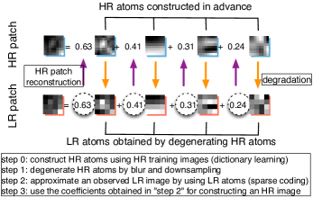
Before performing this single-frame SR, an HR dictionary has to be prepared by an appropriate dictionary learning algorithm with HR training images.
2.2 Multi-frame Super Resolution by Sparse Coding
Suppose low resolution images are observed, all of which are differently degenerated from a high resolution image . Without loss of generality, we assume that the LR image is the target for super resolution, and other LR images are called auxiliary images.
We assume that each patch is exposed by the following image degradation process: for the target patch , the image degradation is modeled by Eq. (1), and for auxiliary patch pairs , observation model
| (5) |
is assumed, where is the parallel shift and clipping operator corresponds to the -th LR patch, which is explained later. We note that can be not identical for different images , but they are assumed to be identical for the sake of simplicity, and we concentrate on estimating for different observations.
In our multi-frame SR, firstly, the target patch is extracted from the target image . Then we consider estimating the shift of the -th image . We can roughly estimate the displacement of the target patch in the auxiliary image by sub-pixel-level accuracy matching in the LR space. To avoid the negative effect at the non-overlapping region and to use the informative area only, the pixels completely included in the placed target patch is extracted as the -th LR patch . Since the target patch is represented by a vector of length , the size of patch in -dimensional expression is . On the other hand, the boundary-clipped patch is of size .
Once are estimated, the image SR based on sparse coding is straight-forward. With the shift and clipping of auxiliary patches , the LR dictionaries correspond to the observations are stacked to construct a stacked LR dictionary:
| (6) |
This dictionary is used to approximate the stacked LR patch
| (7) |
by sparse coding, namely, the HR estimate is given by
| (8) | ||||
| (9) |
Each atom in the HR dictionary is shifted and clipped to an atom of size by the action of , then blurred, down-sampled by the action of to form corresponding LR atoms . Each block of the stacked dictionary in Eq. (6) is composed of LR atoms obtained in this manner.
3 Approximation of Displacements by Pixel-Level Shifts
As discussed in the previous section, the main problem of multi-frame SR is reduced to the problem of estimating shift and clipping operators . In the following, we consider enhancing the resolution of the magnification factor . Since the LR target patch is represented by a square with pixels on a side, the corresponding HR patch is a square with pixels, namely, a vector of size .
For estimating , we consider the upper left most point of the -th auxiliary patch as the origin of the shift, which is on the grid of the -th LR image . We consider the displacement of the target LR patch with HR accuracy in order to achieve satisfactory result, that means placing the target LR patch on the LR image by using sub-pixel level matching. Let the upper left nearest grid point from the origin in the -th LR image be , and the upper left most point of the placed target patch be .
There are two cases of displacement: pixel-level parallel shifts in the HR image space, and others. In the former case where are both integers, the LR dictionary for the auxiliary patch can be simply constructed by clipping the corresponding areas from the HR dictionary and degradation with . Those LR dictionaries of pixel-level parallel shifts are denoted by , and referred to as the LR base dictionaries henceforth. In the latter case, we assume that relative displacement of the auxiliary patch is well-approximated by a linear combination of pixel-level parallel translation in the HR space. Namely, estimating shift and clipping operators is reduced to estimating the combination coefficients for possible parallel translations. The -th block of the LR dictionary in Eq. (6) is then given by
where the LR base dictionaries are common to all of LR observations, and different observation is represented by different coefficients .
In our previous work [8], we took a 2-step procedure for multi-frame SR. That is, firstly we estimate the parameters by using the 2D simultaneous block matching method proposed in [17] because of its computational efficiency. Then, we construct the stacked LR dictionary in Eq. (6) and stacked LR patches in Eq. (7), and the HR patch is obtained by sparse coding. In this work, instead of the 2-step procedure, we propose a novel approach for estimating the sub-pixel level accuracy shifts through a common optimization objective to spares coding.
4 Double Sparsity for Image Super Resolution
In this section, we formalize the proposed method for estimating both displacements of LR images and coefficients for sparse coding.
4.1 Problem Formulation
We start with showing that the stacked LR patches in Eq.(7) is approximated by a bi-linear form. This is done by expressing the stacked dictionary in Eq. (6) as
| (10) |
where is the Kronecker product, is defined by
is defined by
and is the unit matrix of an appropriate size.
Then, the approximation of an LR patch is denoted by
| (11) | ||||
| (12) | ||||
| (13) |
where is the column-span vectorization operator. In the above expression, is the coefficient vector of sparse coding, and is the shift vector of LR observations with sub-pixel level shifts in the HR space. We will estimate and from the observed LR patches. Then, the estimated coefficient is used for reconstructing the HR image as .
The optimization problem to be solved is
| (14) | |||
| (15) |
where denote the vector of all ones. The regularization term imposes sparsity for representing observed signals by linear combinations of atoms. The inequality encodes a constraint that the sum of coefficients for interpolation is less than or equal to one for each image. Here the matrix is defined by
| (16) |
Together with the non-negativity constraint , the constraints and constitute the -norm like constraints with non-negativity, which also produces sparse solutions not only for but also for .
4.2 Optimization method
We solve the optimization problem (14). Since it is intractable to find a closed-form solution for the problem (14) on both and , we alternatingly solve the problem with respect to with a fixed and with respect to with a fixed .
First of all, using only the target LR patch , we initialize the coefficient by solving the following optimization problem,
| (17) |
which is efficiently solved by using sparse coding algorithms.
By fixing the coefficient , we obtain the combination coefficient for shift operators by
| (18) |
This is a quadratic programing problem, and efficiently solved by using any off-the-shelf solver.
For optimizing with a fixed , we solve the following problem:
| (19) |
This problem is also an instance of the -norm regularized least square optimization problem, which is efficiently solved by using sparse coding algorithms. We iteratively solve these optimization problems (18) and (19) until convergence.
In Algorithm 1, we summarize the proposed algorithm with a pseudo-code. By the operation of ClipByMatching, we estimate the position of the target patch in the auxiliary image and extract the auxiliary patch of size . Also, operations of solving Eqs. (18) and (19) are denoted by SolveDisp and SolveCoeff, respectively.
4.3 Double sparsity structure
It is worth noting that the optimization problem (14) shares the same form with the formulation of double sparsity dictionary learning proposed by [10]. Double sparsity dictionary learning is proposed for bridging the gap between analytic dictionary such as wavelets [18] and learning-based dictionary such MOD [12] and K-SVD [13]. The double sparsity dictionary learning assumes that dictionary atoms themselves have some underlying sparse structure over a set of more fundamental base dictionaries. In our formulation of multi-frame super resolution, the atoms are generated from a sparse combination of fundamental atoms derived by pixel-level shifting and degenerating the HR atoms. A schematic diagram of the double sparsity structure in our formulation is shown in Fig. 2.
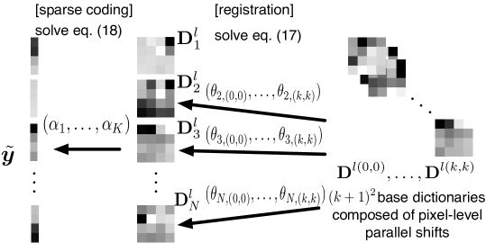
By modeling the shift operation by a set of base shift operators, we obtained a natural and simple formulation of the multi-frame super resolution based on sparse coding.
5 Experimental Results
In this section, we demonstrate the super-resolution results on some sets of still images and some sets of images from movies.
5.1 Application to still images
We suppose observed LR images are generated from an HR image through parallel translations, blurring, down-sampling, and addition of noises. The parallel translations are imitated by shifting the HR image. The degree of vertical and horizontal shifts are randomly sampled from a uniform distribution in . The blurring operation is realized by convolution of -pixel Gaussian filter with the standard deviation . The blurred and shifted images are then down-sampled by the factor three. Finally, noises sampled from are added to generate LR observation images. In our experiments, both the intensity of the blur and the noise are supposed to be given. In our proposed algorithm, we iteratively solve the quadratic programming (18) and the sparse coding problem (19). We observed that the algorithm converged in less than three iterations, hence we fix the iteration number to three in all of the experiments. In our experiments, we magnify the input LR images by a factor of three for all cases. We used five LR images to estimate an HR images, i.e., .
We compare the proposed method to seven conventional methods. The first method is bi-cubic interpolation. This method is simple and regarded as a baseline for SR. The second and third methods are Single-Frame Joint Dictionary Learning (SF-JDL; [6]) and Adaptive Sparse Domain Selection (ASDS; [19]). These methods are considered as state-of-the-art single-frame SR methods with publicly available software implementations. The fourth method is the one proposed by [20], which is a multi-frame SR method based on joint dictionary learning. We refer to this method as MF-JDL (Multi-Frame super resolution based on Joint Dictionary Learning). The other two methods are representative methods in reconstruction-based SR in the literature. In [21], a multi-frame SR method based on regularization in the form of Bilateral Total Variation (BTV) is proposed. Because of its performance and simplicity, the method have become one of the most commonly cited papers in the field of multi-frame SR. BTV is further improved in [22], in which the method based on regularization by Locally Adaptive Bilateral Total Variation (LABTV) is proposed. In this paper, these two reconstruction-based methods are referred to as BTV and LABTV, respectively. Finally, we also use the multi-frame SR method based on sparse coding proposed in our previous paper [8], which is referred to as MF-SC.
There are several tuning parameters for each SR methods. To make fair comparison, we first optimize the parameters of each method to maximize PSNR of the image Lena, which is one of the most commonly used benchmark images in the field of image processing. Then, for all other images, we keep using the same parameters which are optimized for Lena.
We use two different gray-scale images (Lena and Cameraman), and three color images (Flower, Girl, and Parthenon) for evaluating the performance of SR methods. When we deal with color images, we first convert the image into YCbCr format, then apply SR methods only to luminance channel (Y). Values of other channels Cb and Cr are simply expanded by bi-cubic interpolation.
We show the experimental results in Fig. 3-Fig. 7. To focus on the difference between our previous method and the newly proposed method, we only show the original images, degraded images, images obtained by MF-SC and those obtained by our proposed method. These figures indicate that the proposed method can generate comparable or better images compared to MF-SC.

|

|
| (a) Observed LR image | (b) Original HR image |

|

|
| (c) MF-SC | (d) Proposed |

|

|
| (a) Observed LR image | (b) Original HR image |

|

|
| (c) MF-SC | (d) Proposed |

|

|
| (a) Observed LR image | (b) Original HR image |

|

|
| (c) MF-SC | (d) Proposed |

|

|
| (a) Observed LR image | (b) Original HR image |

|

|
| (c) MF-SC | (d) Proposed |

|

|
| (a) Observed LR image | (b) Original HR image |

|

|
| (c) MF-SC | (d) Proposed |
For quantitative comparison of SR methods, we use the Peak Signal to Noise Ratio (PSNR) defined as
| (20) |
where MSE is the mean squared error between the original HR image and the estimated HR image, and the higher PSNR indicates the better SR performance. We show PSNR values obtained by various methods in Table 1. For evaluating the PSNR values, we randomly generated sets of shift operators and generated degraded images by adding random observation noises. From each set of observed images, we randomly choose one target image. The only target image is used for single-frame SR, while in multi-frame SR, the remaining images are used as auxiliary LR images. The means and standard deviations of PSNR values are calculated using SR results by each methods. The best and the second best results are shown in bold and underlined styles, respectively.
| Image | Bicubic | SF-JDL | ASDS | MF-JDL | BTV | LABTV | MF-SC | Proposed |
|---|---|---|---|---|---|---|---|---|
| Lena | ||||||||
| Cameraman | ||||||||
| Flower | ||||||||
| Girl | ||||||||
| Parthenon |
As shown in Table 1, the proposed method outperforms other conventional methods in two out of five images ( Cameraman and Flower), and be the second best for Lena. It improved the previous method in two images, being the same in one image, and slightly worth in two images.
5.2 Application to motion pictures
We show experimental results on LR images sequentially captured from movies. From five consecutive LR images, the middle (third in the temporal sequence) image is selected as the target image, and other four are considered as auxiliary images.
The obtained HR images using MF-SC and the proposed method are shown in Fig. 8 and Fig. 9. We also show the obtained PSNR in Table 2 for all methods.

|

|
| (a) Observed LR image | (b) Original HR image |

|

|
| (c) MF-SC | (d) Proposed |

|

|
| (a) Observed LR image | (b) Original HR image |

|

|
| (c) MF-SC | (d) Proposed |
| Bicubic | SF-JDL | ASDS | MF-JDL | BTV | LABTV | MF-SC | Proposed | |
|---|---|---|---|---|---|---|---|---|
| MacArthur | 34.11 | 34.33 | 35.63 | 35.18 | 34.39 | 34.40 | 34.79 | 35.63 |
| (2.69) | (178.08) | (133.78) | (61.72) | (96.17) | (27.70) | (61.74) | ||
| Samurai | 25.36 | 25.97 | 26.66 | 26.12 | 26.16 | 26.07 | 25.90 | 26.49 |
| (2.50) | (211.65) | (138.38) | (62.13) | (96.24) | (30.75) | (59.86) |
From Fig. 8 and Fig. 9, the HR images obtained by the proposed method are clear and have distinct edges compared to the images obtained by MF-SC. From Table 2, PSNRs of the proposed method are the same or lower than ASDS. However, the computational costs of the proposed method are lower than ASDS and other multi-frame SR methods. Although the proposed method requires about double computational cost to our previous method (MF-SC), it significantly improves the quality of reconstructed image in PSNR.
6 Conclusion
In this paper, we discussed multi-frame image super resolution as a combination of distinct problems of image registration and sparse coding. Main contribution of this work is formulating these two problems within a framework of double sparsity dictionary learning. Image registration and sparse coding problems are unified in a single objective function, then registration coefficients and sparse coding coefficients are alternatingly optimized with quadratic programming and l1-norm constraint least squares, respectively, both of which lead sparse estimation of the coefficients. The proposed method improved our previous formulation of multi-frame super resolution for some images. Particularly, images from movies are significantly improved. We mainly explained the proposed super resolution method with an application to image resolution enhancement, however, we consider that our double-sparsity formulation is applicable to enhancement or refinement of multiple observations from a number of inaccurate sensors with appropriate base dictionaries, such as information integration from observations by autonomous mobile robots. Our future work includes application of the proposed method to other signal resolution enhancement, and further improvement of computational efficiency by adopting or developing optimization methods for sparse coding and shift estimation.
Acknowledgment
Part of this work was supported by JSPS KAKENHI No. 25120009 and 26120504.
References
- [1] B. A. Olshausen and D. J. Field. Emergence of simple-cell receptive field properties by learning a sparse code for natural images. Nature, 381:607–609, 1996.
- [2] B. A. Olshausen and D. J. Field. How Close Are We to Understanding V1? Neural Computation, 17:1665–1699, 2005.
- [3] Balas Kausik Natarajan. Sparse approximate solutions to linear systems. SIAM journal on computing, 24(2):227–234, 1995.
- [4] M. Elad. Sparse and Redundant Representations: From Theory to Applications in Signal and Image Processing. Springer, 2010.
- [5] Jianchao Yang, J. Wright, T. Huang, and Yi Ma. Image super-resolution as sparse representation of raw image patches. In Proceedings of the 2008 IEEE Computer Society Conference on Computer Vision and Pattern Recognition (CVPR’08), pages 1–8, 2008.
- [6] Jianchao Yang, John Wright, Tohmas S. Huang, and Yi Ma. Image super-resolution via sparse representation. IEEE Transactions on Image Processing, 19(11):2861–2873, November 2010.
- [7] Roman Zeyde, Michael Elad, and Matan Protter. On single image scale-up using sparse-representations. In Proceedings of the 7th international conference on Curves and Surfaces, pages 711–730, 2010.
- [8] Toshiyuki Kato, Hideitsu Hino, and Noboru Murata. Multi-frame image super resolution based on sparse coding. Neural Networks, 66:64–78, 2015.
- [9] Barbara Zitova and Jan Flusser. Image registration methods: a survey. Image and Vision Computing, 21(11):977 – 1000, 2003.
- [10] Ron Rubinstein, Michael Zibulevsky, and Michael Elad. Double sparsity: Learning sparse dictionaries for sparse signal approximation. Signal Processing, IEEE Transactions on, 58(3):1553–1564, 2010.
- [11] Xin Zhan, Rong Zhang, Dong Yin, Anzhou Hu, and Wenlong Hu. Remote sensing image compression based on double-sparsity dictionary learning and universal trellis coded quantization. In IEEE International Conference on Image Processing, ICIP 2013, Melbourne, Australia, September 15-18, 2013, pages 1665–1669. IEEE, 2013.
- [12] K. Engan, S. O. Aase, and J. Hakon Husoy. Method of optimal directions for frame design. In Proceedings of the Acoustics, Speech, and Signal Processing, 1999. on 1999 IEEE International Conference - Volume 05, ICASSP ’99, pages 2443–2446, Washington, DC, USA, 1999. IEEE Computer Society.
- [13] M. Aharon, M. Elad, and A. Bruckstein. K-SVD: An Algorithm for Designing Overcomplete Dictionaries for Sparse Representation. IEEE Transactions on Signal Processing, 54(11):4311–4322, 2006.
- [14] Y. C. Pati R. Rezaiifar and P. S. Krishnaprasad. Orthogonal matching pursuit: Recursive function approximation with applications to wavelet decomposition. In Proceedings of the 27 th Annual Asilomar Conference on Signals, Systems, and Computers, pages 40–44, 1993.
- [15] Robert Tibshirani. Regression shrinkage and selection via the lasso. Journal of the Royal Statistical Society, Series B, 58:267–288, 1996.
- [16] Honglak Lee, Alexis Battle, Rajat Raina, and Andrew Y. Ng. Efficient sparse coding algorithms. In NIPS, pages 801–808, 2006.
- [17] M. Shimizu and M. Okutomi. Multi-parameter simultaneous estimation on area-based matching. In International Journal of Computer Vision, vol. 67, no. 3, pp. 327-342, May, 2006.
- [18] Ingrid Daubechies. Ten lectures on wavelets. Society for Industrial and Applied Mathematics, Philadelphia, PA, USA, 1992.
- [19] Weisheng Dong, D. Zhang, Guangming Shi, and Xiaolin Wu. Image Deblurring and Super-Resolution by Adaptive Sparse Domain Selection and Adaptive Regularization. IEEE Transactions on Image Processing, 20(7):1838–1857, 2011.
- [20] Peng Wang, Xiyuan Hu, Bo Xuan, Jiancheng Mu, and Silong Peng. Super Resolution Reconstruction via Multiple Frames Joint Learning. In International Conference on Multimedia and Signal Processing (CMSP), volume 1, pages 357–361, 2011.
- [21] S. Farsiu, M.D. Robinson, M. Elad, and P. Milanfar. Fast and Robust Multiframe Super Resolution. IEEE Transactions on Image Processing, 13(10):1327–1344, Oct 2004.
- [22] Xuelong Li, Yanting Hu, Xinbo Gao, Dacheng Tao, and Beijia Ning. A multi-frame image super-resolution method. Signal Process., 90(2):405–414, February 2010.