Distributed Real-Time Power Balancing
in Renewable-Integrated Power Grids
with Storage and Flexible Loads

Abstract

The large-scale integration of renewable generation directly affects the reliability of power grids. We investigate the problem of power balancing in a general renewable-integrated power grid with storage and flexible loads. We consider a power grid that is supplied by one conventional generator (CG) and multiple renewable generators (RGs) each co-located with storage, and is connected with external markets. An aggregator operates the power grid to maintain power balance between supply and demand. Aiming at minimizing the long-term system cost, we first propose a real-time centralized power balancing solution, taking into account the uncertainty of the renewable generation, loads, and energy prices. We then provide a distributed implementation algorithm, significantly reducing both computational burden and communication overhead. We demonstrate that our proposed algorithm is asymptotically optimal as the storage capacity increases and the CG ramping constraint loosens. Moreover, the distributed implementation enjoys a fast convergence rate, and enables each RG and the aggregator to make their own decisions. Simulation shows that our proposed algorithm outperforms alternatives and can achieve near-optimal performance for a wide range of storage capacity.

I Introduction

With increasing environmental concerns, more and more renewable energy sources such as wind and solar are expected to be integrated into the power grids. Renewable generation is often intermittent with limited dispatchability. Thus, its large-scale integration could upset the balance between supply and demand, and affect the system reliability[1].

To mitigate the randomness of renewable generation, one can employ fast-responsive generators such as natural gas, whose services are nevertheless expensive. Alternative solutions include energy storage and flexible loads, which may be less costly and meanwhile more environmentally friendly[2][3]. In particular, storage can be exploited to shift energy across time; many loads, such as thermostatically controlled loads, electric vehicles, and other smart appliances, can be controlled through curtailment or time shift. Together, storage and flexible loads enable adaptive energy absorption and buffering to counter the fluctuation in renewable generation.

In this paper, we investigate the problem of power balancing in a general renewable-integrated power grid with storage and flexible loads, through the coordination of supply, demand, and storage. Practical power systems are typically operated under multiple time scales. To model this, we consider power balancing for each time scale separately (e.g., [4]). More precisely, we focus on energy management within a single time scale and aim at proposing a distributed real-time algorithm for power balancing. Real-time control is mainly motivated by the unpredictability of renewable sources, which can potentially render off-line algorithms inefficient. The distributed implementation is to reduce the computational burden of the system operator and also to limit the communication requirement.

TABLE I: Comparison with existing works

[5]

[6]

[7]

[8]

[9]

[4]

[10]

[11]

[12]

[13]

[14]

[15]

[16]

Proposed

Supply management

Y

Y

Y

Y

Y

Y

Y

Demand management

Y

Y

Y

Y

Y

Y

Y

Y

Storage management

Y

Y

Y

Y

Y

Y

Y

Y

Y

Y

Uncertainty/dynamics

Y

Y

Y

Y

Y

Y

Y

Y

Y

Y

Y

Y

Y

Y

Ramping constraint

Y

Y

Y

Y

Y

Real-time algorithm

Y

Y

Y

Y

Y

Y

Y

Y

Y

Y

Y

Y

Y

Distributed algorithm

Y

Y

Y

Y

Y

Earlier works on power balancing commonly ignore system uncertainty by considering a deterministic operational environment. There are many recent works explicitly incorporating system uncertainty into energy management of power grids. Due to page limitation, we are only able to select some representative papers that are more related to our work. These works emphasize on various issues of the system in energy management (see Table I for a summary). For example, the authors of [5] and [6] consider supply side management by assuming that all loads are uncontrollable, the authors of [7] study demand side management by optimally scheduling non-interruptible and deferrable loads of individual users, and the authors of [4, 8], and [9] propose to employ energy storage to clear power imbalance. In some other works, the authors combine supply side and demand side managements [10], or supply side and storage managements [11], or demand side and storage managements [12, 13, 14].

Among existing works, [15] and [16] are mostly related to our work, in which all three types of energy management (i.e., supply, demand, and storage) are jointly considered for power balancing. However, in [15], although the uncertainty of the renewable generation is considered and characterized by a polyhedral set, the uncertainty of the loads and energy prices is ignored. Moreover, the algorithm is designed for off-line use such as in day-ahead scheduling, and therefore cannot be implemented in real time. In [16], a real-time algorithm is proposed to minimize the cost of a conventional generator (CG) only. Furthermore, the ramping constraint of the CG is not considered in the algorithm design. As we will see in this paper, the incorporation of such a constraint can significantly complicate the analysis of the real-time algorithm. In addition, the energy management there is performed centrally by a system operator.

In this paper, we include all issues listed in Table I when studying the problem of power balancing. In particular, we consider a general power grid supplied by a CG and multiple RGs, and each RG is co-located with an energy storage unit. An aggregator operates the grid by coordinating supply, demand, and storage units to maintain the power balancing. Our goal is to minimize the long-term system cost subject to the operational constraints and the quality-of-service requirement of flexible loads.

Our formulated optimization problem is stochastic in nature, and is technically challenging especially for real-time control. First, owing to the practical operational constraints, such as the finite storage capacity and the CG ramping constraint, the control actions are coupled over time, which complicates the real-time decision making. Second, centralized control of a potentially large number of RGs by the aggregator may lead to large communication overhead and heavy computation. To overcome the first difficulty, we leverage Lyapunov optimization[17] and develop special techniques to tackle our problem. To address the second challenge, we exploit the structure of the optimization problem and employ the alternating direction method of multipliers (ADMM)[18] to offer a distributed algorithm. Our main contribution is summarized as follows.

• We formulate a stochastic optimization problem for power balancing by taking into account all design issues listed in Table I.

• We propose a distributed real-time algorithm for the power balancing optimization problem. We characterize the performance gap of the proposed algorithm away from an optimal algorithm, and show that the proposed algorithm is asymptotically optimal as the storage capacity increases and the CG ramping constraint loosens. The algorithm can be implemented in a distributed way, by which each RG and the aggregator can make their own decisions. The distributed implementation enjoys a fast convergence rate and requires limited communication between the aggregator and each RG.

• We compare the proposed algorithm with alternative algorithms by simulation. We show that our proposed algorithm outperforms the alternatives and is near-optimal even with small energy storage.

Energy storage has been used widely in power grids for combating the variability of renewable generation. A large amount of works have been reported in literature on storage control and the assessment of its role in renewable integration (e.g., [19, 20, 21, 22, 23]). Compared with these references, this paper focuses on the problem of power balancing, and additionally includes the control of flexible loads in energy management. A traditional approach for storage control is to formulate the problem as a linear-quadratic regulator (LQR) (e.g., [20]). Compared with the Lyapunov optimization approach employed in this paper, the LQR approach is different in terms of its application and the derivation of the control action at each time step. Specifically, the LQR approach applies when the system states evolve according to a set of linear equations and the objective function is quadratic. Obtaining the optimal control action analytically is generally hard and requires system statistics. In contrast, the Lyapunov optimization approach has no such requirements on the problem structure, and can additionally deal with long-term time-averaged constraints. Furthermore, in the Lyapunov optimization approach, the control action at each time step is derived by solving an optimization problem with no need for system statistics.

A preliminary version of this work has been presented in [24]. In this paper, we significantly extend [24] in two ways: first, we offer a distributed algorithm for practical implementation; second, we provide more in-depth performance analysis of the proposed algorithm both theoretically and numerically, and reveal insights into the interactions of supply, demand and storage units in maintaining the power balancing of a grid.

The remainder of this paper is organized as follows. In Section II, we describe the system model and formulate the problem of power balancing. In Section III, we propose a real-time algorithm and analyze its performance theoretically. In Section IV, we provide a distributed algorithm for solving the real-time problem. In Section V, we present simulation results. Finally, we conclude and discuss some future directions in Section VI. The main symbols used in this paper are summarized in Table II.

TABLE II: List of Main Symbols

$N$	number of RGs
$l_{b,t}$	requested amount of base loads during time slot $t$
$l_{f,t}$	requested amount of flexible loads during time slot $t$
$l_{m,t}$	total amount of satisfied loads during time slot $t$
$\alpha$	portion of unsatisfied flexible loads
$a_{i}$	renewable generation amount of the $i$-th RG during time slot $t$
$a_{i,\max}$	maximum amount of renewable generation of the $i$-th RG during each time slot
$x_{i,t}$	charging/discharging amount of the $i$-th storage unit during time slot $t$
$|x_{i,\min}|$	maximum discharging amount
$x_{i,\max}$	maximum charging amount
$b_{i,t}$	contributed energy amount by the $i$-th RG during time slot $t$
$s_{i,t}$	energy state of the $i$-th storage unit at the beginning of time slot $t$
$D_{i}(\cdot)$	degradation cost function of the $i$-th storage unit
$g_{t}$	output of the CG during time slot $t$
$g_{\max}$	maximum output of the CG during each time slot
$r$	ramping coefficient
$C(\cdot)$	generation cost function of the CG
$p_{b,t}$	unit buying price of external energy markets at time slot $t$
$p_{s,t}$	unit selling price of external energy markets at time slot $t$
$e_{b,t}$	amount of energy bought from external energy markets during time slot $t$
$e_{s,t}$	amount of energy sold to external energy markets during time slot $t$
$\mathbf{q}_{t}$	system states at time slot $t$
$\mathbf{u}_{t}$	control actions at time slot $t$
$w_{t}$	system cost at time slot $t$

II System Model and Problem Statement

II-A System Model

As shown in Fig. 1, we consider a power grid supplied by one CG (e.g., nuclear, coal-fired, or gas-fired generator) and $N$ RGs (e.g., wind or solar generators). Each RG is co-located with one on-site energy storage unit. The grid is connected to external energy markets and is operated by an aggregator, who is responsible for satisfying the loads by managing energy from various sources. The information flow and the energy flow are also depicted in Fig. 1. Assume that the system operates in discrete time with time slot $t\in\{0,1,2,\cdots\}$. For notational simplicity, throughout the paper we work with energy units instead of power units. The details of each component in the power grid are described below.

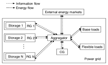
Figure 1: Schematic representation of the considered power grid.

II-A1 Loads

The loads include base loads and flexible loads. The base loads represent critical energy demands such as lighting, which must be satisfied once requested. The flexible loads here represent some controllable energy requests that can be partly curtailed if the energy provision cost is high. At time slot $t$, denote the amount of the total requested base loads by $l_{b,t}\in[l_{b,\min},l_{b,\max}],$ and the amount of the total requested flexible loads by $l_{f,t}\in[l_{f,\min},l_{f,\max}]$. The amounts $l_{b,t}$ and $l_{f,t}$ are generated by users based on their own needs and are considered random. Let the amount of the total satisfied loads be $l_{m,t}$, which should satisfy

$$l_{b,t}\leq l_{m,t}\leq l_{b,t}+l_{f,t}.$$ (1)

The control of flexible loads needs to meet certain quality-of-service requirement. In this work, we impose an upper bound on the portion of unsatisfied flexible loads. Formally, we introduce a long-term time-averaged constraint

$$\limsup_{T\to\infty}\frac{1}{T}\sum_{t=0}^{T-1}\mathbb{E}\left[\frac{l_{b,t}+l_{f,t}-l_{m,t}}{l_{f,t}}\right]\leq\alpha$$ (2)

where $\alpha\in[0,1]$ is a pre-designed threshold with a small value indicating a tight quality-of-service requirement.

II-A2 RG and On-Site Storage

At the $i$-th RG, denote the amount of the renewable generation during time slot $t$ by $a_{i,t}\in[0,a_{i,\max}]$, where $a_{i,\max}$ is the maximum generated energy amount. Due to the stochastic nature of renewable sources, $a_{i,t}$ is random.

We assume that each RG is co-located with one on-site energy storage unit capable of charging and discharging. Denote the charging or discharging energy amount of the $i$-th storage unit during time slot $t$ by $x_{i,t}$, with $x_{i,t}>0$ (resp. $x_{i,t}<0$) indicating charging (resp. discharging). Because of the battery design and hardware constraints, the value of $x_{i,t}$ is bounded as follows:

$$x_{i,\min}\leq x_{i,t}\leq x_{i,\max},\quad(x_{i,\min}<0<x_{i,\max})$$ (3)

where $|x_{i,\min}|$ and $x_{i,\max}$ represent the maximum discharging and charging amounts, respectively. For the $i$-th storage unit, denote its energy state at the beginning of time slot $t$ by $s_{i,t}$. Due to charging and discharging operations, the evolution of $s_{i,t}$ is given by

$$s_{i,t+1}=s_{i,t}+x_{i,t}.$$ (4)

Furthermore, the battery capacity and operational constraints require the energy state $s_{i,t}$ be bounded as follows:

$$s_{i,\min}\leq s_{i,t}\leq s_{i,\max}$$ (5)

where $s_{i,\min}$ is the minimum allowed energy state, and $s_{i,\max}$ is the maximum allowed energy state and can be interpreted as the storage capacity. It is known that fast charging or discharging can cause battery degradation, which shortens battery lifetime [25]. To model this cost on storage, we use $D_{i}(\cdot)$ to represent the degradation cost function associated with the charging or discharging amount $x_{i,t}$.

During every time slot, the RG supplies energy to the aggregator. Denote the amount of the contributed energy by the $i$-th RG during time slot $t$ by $b_{i,t}$. Since the energy flows of the RG should be balanced, we have

$$b_{i,t}=a_{i,t}-x_{i,t},\quad b_{i,t}\geq 0.$$ (6)

In particular, if $x_{i,t}>0$ (charging), the contributed energy $b_{i,t}$ directly comes from the renewable generation; if $x_{i,t}<0$ (discharging), $b_{i,t}$ comes from both the renewable generation and the storage unit.

II-A3 CG

Different from the RGs, the energy output of the CG is controllable. Denote $g_{t}$ as the energy output of the CG during time slot $t$, satisfying

$$0\leq g_{t}\leq g_{\max}$$ (7)

where $g_{\max}$ is the maximum amount of the energy output. Due to the operational limitations of the CG, the change of the outputs in two consecutive time slots is bounded. This is typically reflected by a ramping constraint on the CG outputs [26]. Assuming that the ramp-up and ramp-down constraints are identical, we express the overall ramping constraint as

$$|g_{t}-g_{t-1}|\leq rg_{\max}$$ (8)

where the coefficient $r\in[0,1]$ indicates the tightness of the ramping requirement. In particular, for $r=0$, the CG produces a fixed output over time, while for $r=1$, the ramping requirement becomes non-effective. Furthermore, we denote the generation cost function of the CG by $C(\cdot)$.

II-A4 External Energy Markets

In addition to the internal energy resources, the aggregator can resort to the external energy markets if needed. For example, the aggregator can buy energy from the external energy markets in the case of energy deficit, or sell energy to the markets in the case of energy surplus. At time slot $t$, denote the unit prices of the external energy markets for buying and selling energy by $p_{b,t}\in[p_{b,\min},p_{b,\max}]$ and $p_{s,t}\in[p_{s,\min},p_{s,\max}]$, respectively. To avoid energy arbitrage, the buying price is assumed to be strictly greater than the selling price, i.e., $p_{b,t}>p_{s,t}$. The prices $p_{b,t}$ and $p_{s,t}$ are typically random due to unexpected market behaviors. Denote

$$e_{b,t}\geq 0,\quad e_{s,t}\geq 0$$ (9)

as the amounts of the energy bought from and sold to the external energy markets during time slot $t$, respectively. The overall system balance requirement is

$$\textstyle{g_{t}+e_{b,t}+\sum_{i=1}^{N}b_{i,t}=e_{s,t}+l_{m,t}.}$$ (10)

II-B Problem Statement

The aggregator operates the power grid and aims to minimize the long-term time-averaged system cost by jointly managing supply, demand, and storage units. With an increasing integration of renewable generation and energy storage into power grids, the business models of electric utilities are evolving. From the study in [27], one suggested model of future electric utilities is termed as “energy services utility.” Such utilities are expected to provide similar services as those described in Section II-A. Precisely, besides serving loads, these utilities would actively provide a platform for demand response, manage generation assets, and coordinate energy sales with external energy markets.

We define the control actions at time slot $t$ by

$$\mathbf{u}_{t}{\triangleq}\left[\mathbf{b}_{t},\mathbf{x}_{t},l_{m,t},g_{t},e_{b,t},e_{s,t}\right]$$

where $\mathbf{b}_{t}{\triangleq}[b_{1,t},\cdots,b_{N,t}]$ and $\mathbf{x}_{t}{\triangleq}[x_{1,t},\cdots,x_{N,t}]$. The system cost at time slot $t$ includes the costs of all RGs and the CG, and the cost for exploiting the external energy markets, given by:

$$w_{t}{\triangleq}C(g_{t})+p_{b,t}e_{b,t}-p_{s,t}e_{s,t}+\sum_{i=1}^{N}D_{i}(x_{i,t}).$$

Based on the system model described in Section II-A, we formulate the problem of power balancing as a stochastic optimization problem below.

$$\textbf{P1}:\;\min_{\{\mathbf{u}_{t}\}}\quad \limsup_{T\to\infty}\;\frac{1}{T}\sum_{t=0}^{T-1}\mathbb{E}[w_{t}]\quad\textrm{s.t.}\quad\eqref{conl}-\eqref{conmbl}$$

where the expectations in the objective and (2) are taken over the randomness of the system states $\mathbf{q}_{t}{\triangleq}[\mathbf{a}_{t},l_{b,t},l_{f,t},p_{b,t},p_{s,t}]$ where $\mathbf{a}_{t}{\triangleq}[a_{1,t},\cdots,a_{N,t}]$, and the possible randomness of the control actions.

To keep mathematical exposition simple, we assume that the cost functions $C(\cdot)$ and $D_{i}(\cdot)$ are continuously differentiable and convex. This assumption is mild since many practical costs can be well approximated by such functions. Denote the derivatives of $C(\cdot)$ and $D_{i}(\cdot)$ by $C^{\prime}(\cdot)$ and $D^{\prime}_{i}(\cdot)$, respectively. Based on the assumption, we have the derivative $C^{\prime}(g_{t})\in[C^{\prime}_{\min},C^{\prime}_{\max}],\forall g_{t}\in[0,g_{\max}]$, and $D_{i}^{\prime}(x_{i,t})\in[D^{\prime}_{i,\min},D^{\prime}_{i,\max}],\forall x_{i,t}\in[x_{i,\min},x_{i,\max}]$.

Remarks: Compared to a practical power system, the model considered in Section II-A is simplified, in which power losses, network constraints, and some other practical operational constraints are ignored. Despite the simplifications, we will show that the proposed formulation leads to an implementable control algorithm with a provable performance bound on suboptimality. For future work, we will consider incorporating more practical power system constraints into the problem formulation.

III Real-Time Algorithm for Power Balancing

Solving P1 is challenging, due to the stochastic nature of the system, as well as constraints (2), (5), and (8), resulting in coupled control actions over time. In this section, we propose a real-time algorithm for P1 and analyze its performance theoretically.

III-A Description of Real-Time Algorithm

To propose a real-time algorithm, we employ the Lyapunov optimization approach[17]. Lyapunov optimization can be used to transform some long-term time-averaged constraints such as (2) into queue stability constraints, and to provide efficient real-time algorithms for complex dynamic systems. Unfortunately, the time-coupled constraints (5) and (8) are not time-averaged constraints, but are hard constraints required at each time slot. Therefore, the Lyapunov optimization framework cannot be directly applied. To overcome this difficulty, we take a relaxation step and propose the following relaxed problem:

$$\textbf{P2}:\;\min_{\{\mathbf{u}_{t}\}}\quad \limsup_{T\to\infty}\;\frac{1}{T}\sum_{t=0}^{T-1}\mathbb{E}[w_{t}]$$

s.t. $$\eqref{conl}-\eqref{conx},\eqref{conb},\eqref{cong},\eqref{cone},\eqref{conmbl},$$

$$\lim_{T\to\infty}\;\frac{1}{T}\sum_{t=0}^{T-1}\mathbb{E}[x_{i,t}]=0,\quad\forall i.$$ (11)

Compared with P1, in P2 the energy state constraints (4) and (5) are replaced with a new time-averaged constraint (11), and the ramping constraint (8) is removed. It can be shown that P2 is indeed a relaxation of P1 (see Appendix A).

The above relaxation step is crucial and enables us to work under the standard Lyapunov optimization framework. However, we emphasize that, giving solution to P2 is not our purpose. Instead, the significance of proposing P2 is to facilitate the design of a real-time algorithm for P1 and the performance analysis. Note that due to this relaxation, the solution to P2 may be infeasible to P1. Motivated by this concern, we next provide a real-time algorithm which can guarantee that all constraints of P1 are satisfied.

To meet constraint (2), we introduce a virtual queue backlog $J_{t}$ evolving as follows:

$$J_{t+1}=\max\{J_{t}-\alpha,0\}+\frac{l_{b,t}+l_{f,t}-l_{m,t}}{l_{f,t}}.$$ (12)

From (12), the virtual queue $J_{t}$ accumulates the portion of unsatisfied flexible loads. It can be shown that maintaining the stability of $J_{t}$ is equivalent to satisfying constraint (2) [17]. We initialize $J_{t}$ as $J_{0}=0$.

At time slot $t$, define a vector $\mathbf{\Theta}_{t}{\triangleq}[s_{1,t},\ldots,s_{N,t},J_{t}]$, which consists of the energy states of all storage units and the virtual queue backlog $J_{t}$. Using $\mathbf{\Theta}_{t}$, we define a Lyapunov function $L(\mathbf{\Theta}_{t}){\triangleq}\frac{1}{2}J_{t}^{2}+\frac{1}{2}\sum_{i=1}^{N}(s_{i,t}-\beta_{i})^{2},$ where $\beta_{i}$ is a perturbation parameter designed for ensuring the boundedness of the energy state, i.e., constraint (5). In addition, we define the one-slot conditional Lyapunov drift as $\Delta(\mathbf{\Theta}_{t}){\triangleq}\mathbb{E}\left[L(\mathbf{\Theta}_{t+1})-L(\mathbf{\Theta}_{t})|\mathbf{\Theta}_{t}\right]$. Instead of directly minimizing the system cost objective, we consider the drift-plus-cost function given by $\Delta(\mathbf{\Theta}_{t})+V\mathbb{E}[w_{t}|\mathbf{\Theta}_{t}]$. It is a weighted sum of $\Delta(\mathbf{\Theta}_{t})$ and the system cost at time slot $t$ with $V$ serving as the weight.

In our algorithm design, we first consider an upper bound on the drift-plus-cost function (see Appendix B for the upper bound), and then formulate a real-time optimization problem to minimize this upper bound at every time slot $t$. As a result, at each time slot $t$, we have the following optimization problem:

$$\textbf{P3}:\;\min_{\mathbf{u}_{t}}\quad \left[\sum_{i=1}^{N}VD_{i}(x_{i,t})+(s_{i,t}-\beta_{i})x_{i,t}\right]+VC(g_{t})$$

$$+Vp_{b,t}e_{b,t}-Vp_{s,t}e_{s,t}-\frac{J_{t}}{l_{f,t}}l_{m,t}$$

s.t. $$\eqref{conl},\eqref{conx},\eqref{conb}-\eqref{conmbl}.$$

We will show in Section III-B that the design of the real-time problem P3 can lead to some analytical performance guarantee. Moreover, to ensure the feasibility of $g_{t}$, we take a natural step and move the ramping constraint (8) back into P3.

Since $D_{i}(\cdot)$ and $C(\cdot)$ are convex, P3 is a convex optimization problem and can be efficiently solved by standard convex optimization software packages. Denote an optimal solution of P3 at time slot $t$ by $\mathbf{u}_{t}^{*}{\triangleq}\left[\mathbf{b}_{t}^{*},\mathbf{x}_{t}^{*},l_{m,t}^{*},g_{t}^{*},e_{b,t}^{*},e_{s,t}^{*}\right]$. At each time slot, after obtaining $\mathbf{u}_{t}^{*}$, we update $s_{i,t},\forall i$, and $J_{t}$ based on their evolution equations.

In the following proposition we prove that, despite the relaxation to P2, by appropriately designing the perturbation parameter $\beta_{i}$ we can ensure the boundedness of the energy states and hence the feasibility of the control actions $\{\mathbf{u}_{t}^{*}\}$ to P1.

Proposition 1

For the $i$-th storage unit, set the perturbation parameter $\beta_{i}$ as

$$\beta_{i}{\triangleq}V(p_{b,\max}+D^{\prime}_{i,\max})-x_{i,\min}+s_{i,\min}$$ (13)

where $V\in(0,V_{\max}]$ with

$$V_{\max}{\triangleq}\min_{1\leq i\leq N}\left\{\frac{s_{i,\max}-s_{i,\min}+x_{i,\min}-x_{i,\max}}{p_{b,\max}-p_{s,\min}+D^{\prime}_{i,\max}-D^{\prime}_{i,\min}}\right\}.$$ (14)

Then the control actions $\{\mathbf{u}_{t}^{*}\}$ derived by solving P3 at each time $t$ are feasible to P1.

Proof:

See Appendix C. ∎

Remarks: For $V_{\max}$ in (14) to be positive, the range of the energy state should be larger than the sum of the maximum charging and discharging amounts. This is generally true if the length of each time interval is not too long, for example, up to several minutes.

We summarize the proposed real-time algorithm in Algorithm 1. We can see that, Algorithm 1 is simple and does not require any statistics of the system states. The latter feature is especially desirable in practice, where accurate statistics of the system states are difficult to obtain but instantaneous observations are readily available.

Initialize $J_{0}=0$. At each time slot $t$, the aggregator executes the following steps sequentially.

1. Observe the system states $\mathbf{q}_{t}$, energy states $s_{i,t},\forall i,$ and queue backlog $J_{t}$.

2. Solve P3 and obtain an optimal solution $\mathbf{u}_{t}^{*}$.

3. Use $\mathbf{u}_{t}^{*}$ to update $s_{i,t},\forall i,$ and $J_{t}$ based on (4) and (12), respectively.

Algorithm 1 Real-time algorithm for power balancing.

III-B Performance Analysis

We now analyze the solution provided by Algorithm 1 with respect to P1. Under Algorithm 1, to emphasize the dependency of the cost objective value on the ramping coefficient $r$ and the control parameter $V$, we denote the achieved cost objective value by $w^{*}(r,V)$. Denote the minimum cost objective value of P1 by $w^{\textrm{opt}}(r)$, which only depends on $r$. The main results are summarized in the following theorem.

Theorem 1

Assume that the random system states $\mathbf{q}_{t}$ of the grid are i.i.d. over time. Then under Algorithm 1 we have

1. $\textstyle{w^{*}(r,V)-w^{\textrm{opt}}(r)\leq(1-r)g_{\max}\max\{p_{b,\max},C^{\prime}_{\max}\}}$ $+B/V$, where $B$ is a constant defined by $B{\triangleq}\frac{1}{2}(1+\alpha^{2})+\frac{1}{2}\sum_{i=1}^{N}\max\{x_{i,\min}^{2},x_{i,\max}^{2}\}$; and

2. $w^{\textrm{opt}}(r)\geq w^{*}(1,V)-B/V$.

Proof:

See Appendix D. ∎

Remarks:

• Theorem 1.1 characterizes an upper bound on the performance gap away from $w^{\textrm{opt}}(r)$. The upper bound has two terms reflecting the ramping constraint and storage capacity limitation. It indicates that Algorithm 1 provides an asymptotically optimal solution as the ramping constraint becomes loose (i.e., $r\to 1$) and the control parameter $V$ increases (or the storage capacity $s_{i,\max}$ increases based on the $V_{\max}$ expression in (14)). This is consistent with our intuition. Using this insight, in order to minimize the gap to the minimum system cost, we should set $V=V_{\max}$ in Algorithm 1.

• Theorem 1.2 provides a lower bound on $w^{\textrm{opt}}(r)$ in terms of the special case where the ramping constraint is loose, i.e., $r=1$. Since solving P1 to obtain the minimum objective value $w^{\textrm{opt}}(r)$ is difficult, we will use this lower bound as a benchmark for performance comparison in simulation. The gap between the performance under Algorithm 1 and this lower bound serves as an upper bound on the performance gap between Algorithm 1 and an optimal control algorithm.

• The i.i.d. assumption of the system states $\mathbf{q}_{t}$ can be relaxed to accommodate $\mathbf{q}_{t}$ evolving based on a finite state irreducible and aperiodic Markov chain. Similar conclusions can be shown, which are omitted for brevity.

In the above analysis, the storage capacity $s_{i,\max}$ is assumed to be fixed, so that the control parameter $V$ should be upper bounded by $V_{\max}$ in (14) for ensuring the feasibility of the solution. Alternatively, if the storage capacity can be designed, the question is what its value should be in order to achieve certain required performance. In the following proposition, we provide an answer to this question by giving an upper bound on the energy state $s_{i,t}$ (hence an upper bound on the minimum required energy capacity) for an arbitrary positive $V$ that can be greater than $V_{\max}$.

Proposition 2

For any $V>0$, the energy state $s_{i,t}$ of the $i$-th storage unit at time slot $t$ under Algorithm 1 satisfies $s_{i,t}\in[s_{i,\min},s_{i,\textrm{up}}]$ where

$$s_{i,\textrm{up}}{\triangleq} V(p_{b,\max}-p_{s,\min}+D^{\prime}_{i,\max}-D^{\prime}_{i,\min})$$

$$+x_{i,\max}-x_{i,\min}+s_{i,\min}.$$ (15)

Proof:

See Appendix E. ∎

The expression of $s_{i,\textrm{up}}$ in (15) is informative and reveals some insights into the dependency of the design of the storage capacity on some system parameters. First, $s_{i,\textrm{up}}$ increases linearly with the control parameter $V$. Second, $s_{i,\textrm{up}}$ is larger if the energy prices are more volatile or the marginal degradation cost increases fast. Third, the minimum $s_{i,\textrm{up}}$ is given by $-x_{i,\min}+x_{i,\max}+s_{i,\min}$ if we have $p_{b,\max}=p_{s,\min}$ and $D^{\prime}_{i,\max}=D^{\prime}_{i,\min}$.

Other properties regarding flexible loads and external transactions are summarized in the following proposition.

Proposition 3

Under Algorithm 1 the following results hold.

1. The queue backlog $J_{t}$ is uniformly bounded from above as $J_{t}\leq Vp_{b,\max}l_{f,\max}+1.$

2. The amounts of the external transactions $e_{b,t}^{*}$ and $e_{s,t}^{*}$ satisfy $e_{b,t}^{*}e_{s,t}^{*}=0$.

Proof:

See Appendix F. ∎

Remarks:

• In Proposition 3.1, the upper bound of $J_{t}$ is deterministic and does not change over time. Moreover, the fact that $J_{t}$ is upper bounded implies that the accumulated portion of unsatisfied flexible loads is upper bounded.

• Proposition 3.2 implies that the aggregator does not buy energy from or sell energy to the external energy markets simultaneously.

III-C Discussion on Multiple CGs

In the current system model, apart from multiple renewable generators, we incorporate one conventional generator (CG) into the supply side. If there are multiple CGs with the same characteristics, i.e., the same maximum output $g_{\max}$, ramping coefficient $r$, and cost function $C(\cdot)$, for mathematical analysis, we can combine them into one generator. In this case, the current mathematical framework and the performance analysis apply directly with the combined generator. The output of each individual CG can then be obtained by dividing the output of the combined generator equally over all individual ones. On the other hand, if these CGs have heterogeneous characteristics and therefore cannot be combined into one, the proposed algorithm can still be used. In particular, in the original problem P1, we would have constraints (7) and (8) for each individual generator; the total output of the generators in (10) is $\sum_{j=1}^{M}g_{j,t}$; and the total cost of the generators is $\sum_{j=1}^{M}C_{j}(g_{i,t})$. The resultant relaxed problem P2 would be similar to the current one, in which the ramping constraint (8) is removed for each individual CG. For the real-time algorithm, the formulation of the per-slot optimization problem follows the current mathematical framework. Moreover, distributed implementation of the algorithm (shown later in Section IV) can be developed using the same approach we propose.

IV Distributed Implementation of Real-Time Algorithm

At each time slot, our proposed algorithm (Algorithm 1) can be implemented by the aggregator centrally. However, the RGs may not be willing to relinquish direct control of storage or to offer private information to the aggregator. In addition, the computational complexity of centralized control would grow quickly as the number of RGs increases. In this section, we provide a distributed algorithm for solving P3, by which each RG and the aggregator can make their own control decisions.

IV-A Distributed Algorithm Design

To facilitate the algorithm development, we first transform P3 into an equivalent problem. For notational simplicity we drop the time index $t$. We define a new optimization vector $\mathbf{y}{\triangleq}[y_{1},\cdots,y_{N+4}]$, which relates to the optimization variables of P3 by $y_{i}=x_{i}$ for $1\leq i\leq N,y_{N+1}=l_{m},y_{N+2}=-g,y_{N+3}=-e_{b},$ and $y_{N+4}=e_{s}$. Then, the objective of P3 can be rewritten as the sum of certain functions of each $y_{i}$, which are denoted by $F_{i}(y_{i})$ but whose details are omitted for brevity. In addition, we replace $b_{i}$ in the constrains of P3 by $a_{i}-y_{i}$ for $1\leq i\leq N$ based on constraint (6). Consequently, P3 can be rewritten in a generic form P4 below.

P4: $$\min_{\mathbf{y}}\quad\sum_{i=1}^{N+4}F_{i}(y_{i})\quad\quad\textrm{s.t.}\;y_{i}\in\mathcal{Y}_{i},\forall i,\;\sum_{i=1}^{N+4}y_{i}=\sum_{i=1}^{N}a_{i}$$

where the constraint sets $\{\mathcal{Y}_{i}\}$ are derived from constraints (1), (3), and (6)-(9), given by $\mathcal{Y}_{i}{\triangleq}[x_{i,\min},\min\{a_{i},x_{i,\max}\}],i\in\{1,\cdots,N\},\mathcal{Y}_{N+1}{\triangleq}[l_{b},l_{b}+l_{f}],\mathcal{Y}_{N+2}{\triangleq}\big{[}-\min\{g_{\max},g_{t-1}+rg_{\max}\},-\max\{g_{t-1}-rg_{\max},0\}\big{]},\mathcal{Y}_{N+3}{\triangleq}(-\infty,0],$ and $\mathcal{Y}_{N+4}{\triangleq}[0,+\infty)$.

Next, we introduce an auxiliary vector $\mathbf{z}$ as a copy of $\mathbf{y}$ and further transform P4 into the following equivalent problem.

$$\textbf{P5:}\;\min_{\mathbf{y},\mathbf{z}}\quad \sum_{i=1}^{N+4}\big{[}F_{i}(y_{i})+\mathbf{1}(y_{i}\in\mathcal{Y}_{i})\big{]}+\mathbf{1}\Big{(}\sum_{i=1}^{N+4}z_{i}=\sum_{i=1}^{N}a_{i}\Big{)}$$

s.t. $$\mathbf{y}-\mathbf{z}=0$$ (16)

where $\mathbf{1}(\cdot)$ is an indicator function that equals $0$ if the enclosed event is true and infinity otherwise. Through the above transformations, the optimization problem P5 now fits the two-block form of the alternating direction method of multipliers (ADMM) [18], enabling us to develop the distributed optimization algorithm.

Following a general ADMM approach[18], we associate the equality constraint (16) in P5 with dual variables $\mathbf{d}{\triangleq}[d_{1},\cdots,d_{N+4}]$. Denote $y_{i}^{k},z_{i}^{k},$ and $d_{i}^{k}$ as the respective variable values at the $k$-th iteration. Then, based on ADMM, these values are updated as follows.

$$y_{i}^{k+1}=\arg\!\min_{y_{i}}\left\{F_{i}(y_{i})+\frac{\rho}{2}\big{(}y_{i}-z_{i}^{k}+\frac{d_{i}^{k}}{\rho}\big{)}^{2}|y_{i}\in\mathcal{Y}_{i}\right\},\forall i,$$ (17)

$$\mathbf{z}^{k+1}=\arg\!\min_{\mathbf{z}}\left\{\sum_{i=1}^{N+4}\big{(}z_{i}-\frac{d_{i}^{k}}{\rho}-y_{i}^{k+1}\big{)}^{2}|\sum_{i=1}^{N+4}z_{i}=\sum_{i=1}^{N}a_{i}\right\},$$ (18)

$$d_{i}^{k+1}=d_{i}^{k}+\rho(y_{i}^{k+1}-z_{i}^{k+1}),\forall i$$ (19)

where $\rho>0$ is a penalty parameter, which needs to be carefully adjusted for good convergence performance[18].

After further algebraic manipulation (see Appendix G), we can eliminate the vectors $\mathbf{z}$ and $\mathbf{d}$ and simplify the updates (17)-(19) as follows:

$$y_{i}^{k+1}=\arg\!\min_{y_{i}}\left\{F_{i}(y_{i})+\frac{\rho}{2}\big{(}y_{i}-v_{i}^{k})^{2}|y_{i}\in\mathcal{Y}_{i}\right\},\forall i,$$ (20)

$$d^{k+1}=d^{k}+\rho\left(\overline{y}^{k+1}-\frac{1}{N+4}\sum_{i=1}^{N}a_{i}\right).$$ (21)

In (20), we have $v_{i}^{k}{\triangleq}y_{i}^{k}-\overline{y}^{k}-\frac{d^{k}}{\rho}+\frac{1}{N+4}\sum_{i=1}^{N}a_{i}$ where $\overline{y}^{k}{\triangleq}\frac{1}{N+4}\sum_{i=1}^{N+4}y_{i}^{k}$ and $d^{k}$ is a scalar updated as in (21).

Remarks: Following the proof of Theorem 2 in [28], we can show that the above updates lead to a worst-case convergence rate $O(1/k)$. Compared with the subgradient-based algorithm, which presents a worst-case convergence rate $O(1/\sqrt{k})$, the proposed distributed algorithm is much faster and thus is well suited for real-time implementation.

IV-B Distributed Implementation

Now we discuss the implementation of the proposed distributed algorithm in terms of both computation and communication. In Fig. 2, we depict the information flow between the aggregator and the RGs for the updates in (20) and (21) at the $(k+1)$-th iteration.

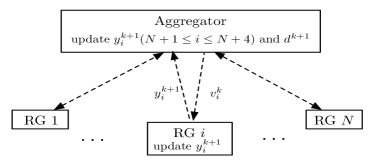
Figure 2: Information flow of distributed implementation.

Note that the minimization problems in (20) can be solved individually at each RG $i$ for $1\leq i\leq N$, and at the aggregator for $N+1\leq i\leq N+4$, while the update in (21) can be computed by the aggregator. At the initial iteration $k=0$, each RG $i$ needs to send its renewable generation amount $a_{i}$ to the aggregator. At each iteration, the aggregator sends a signal $v_{i}^{k}$ to each RG $i$. Then RG $i$ obtains the update $y_{i}^{k+1}$ and sends it back to the aggregator. We see that, the RGs do not have to release any other private information to the aggregator, and the required information exchange is limited to one variable in each direction per RG.

Note that the minimization problems in (20) are all strictly convex and admit a unique (and sometimes closed-form) solution. Furthermore, effectively, only one dual variable is required to be updated in (21). This is because the transformation from P3 to P4 by introducing the new optimization vector $\mathbf{y}$ permits all dual variables to share the same updating structure, hence reducing the number of the effective dual updates as well as simplifying the calculation.

V Simulation Results

In this section, we evaluate the proposed real-time algorithm and compare it with alternatives using an idealized but representative power grid setup.

V-A Simulation Setup

Unless otherwise specified, the following parameters are set as default. The length of each time slot is $10$ min. The amounts of the base loads $l_{b,t}$ and the flexible loads $l_{f,t}$ are uniformly distributed between $5$ and $25$ kWh, and the portion of unsatisfied flexible loads $\alpha$ is $0.5$. The aggregator is connected with $N=30$ RGs. For each on-site storage unit, we set the maximum discharging and charging amounts to be $1.1$ kWh by assuming that the discharging and charging rate is $6.6$ kW (three-phase, level II)[29]. Since the model of the degradation cost function of storage is usually proprietary and unavailable, in simulation, we set $D_{i}(x)=10x^{2}$ as an example. The renewable generation $a_{i,t}$ is uniformly distributed between $0$ and $1.1$ kWh. For the CG, we set the generation cost function to be $C(x)=8x$, the maximum output $g_{\max}=50$ kWh, and the ramping coefficient $r=0.1$. The unit buying energy price $p_{b,t}$ is uniformly distributed between $10$ and $12$ cents/kWh, which is around the current mid-peak energy price in Ontario[30]. The unit selling energy price $p_{s,t}$ is uniformly distributed between $4$ and $6$ cents/kWh, which is slightly below the current off-peak energy price in Ontario[30]. The control parameter $V$ is set to $1$, $s_{i,\min}=0$, and $s_{i,\max}$ is given by (15).

V-B Benchmark Algorithms

As discussed in Section I, compared with previous works (e.g., [5, 6, 7, 8, 9, 4, 10, 11, 12, 13, 14, 15, 16]), this paper is built on a more general system model in which all issues listed in Table I are incorporated into the problem formulation. Therefore, mathematically, the problem we study is new and different from all previous ones. As a result, the proposed algorithm cannot be directly compared with the algorithms presented in [5, 6, 7, 8, 9, 4, 10, 11, 12, 13, 14, 15, 16]. To overcome this difficulty, we employ two alternative algorithms as well as the lower bound on the minimum system cost derived in Theorem 1.2 for comparison.

The first alternative is a greedy algorithm, which only minimizes the current system cost. The optimization problem of the greedy algorithm at time slot $t$ is formulated as follows:

$$\min_{\mathbf{u}_{t}}\quad w_{t}$$

s.t. $$\eqref{conx},\eqref{conb}-\eqref{conmbl},$$

$$\textstyle{l_{b,t}+(1-\alpha)l_{f,t}\leq l_{m,t}\leq l_{b,t}+l_{f,t},}$$

$$\textstyle{-s_{i,t}\leq x_{i,t}\leq s_{i,\max}-s_{i,t}.}$$

The second alternative is suggested mainly to show the effect of the ramping constraint. In particular, at each time slot $t$, we solve an optimization problem that is the same as P3 except without the ramping constraint (8). Therefore, the resultant CG output may be infeasible to P1. To maintain feasibility, whenever the CG output violates the ramping constraint, the aggregator only uses the external energy markets to augment the CG output. We call it “naive algorithm” below.

V-C Comparison under Parameters $V$ and $\alpha$

In Fig. 5, we depict the time-averaged system cost under various values of the control parameter $V$. For the proposed algorithm, the system cost drops quickly and then remains stable as it drops close to the lower bound. This observation demonstrates the efficiency of the algorithm and implies that using small storage may be enough to achieve near-optimal performance. In contrast, the performance of the greedy algorithm barely changes with $V$. In particular, the system cost under the greedy algorithm is about $1.7$ times that under the proposed algorithm when $V\geq 0.1$.

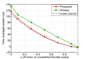
Figure 3: System cost vs. control parameter $V$.

Figure 4: System cost vs. portion of unsatisfied flexible loads $\alpha$.

Figure 5: System cost vs. ramping coefficient $r$ (small loads).

In Fig. 5, we illustrate the effect of $\alpha$, the portion of unsatisfied flexible loads. As expected, the system cost goes down as $\alpha$ rises, since less load is to be satisfied. For the proposed algorithm, the marginal system cost decreases with $\alpha$, which indicates that the benefit of curtailing loads keeps on falling. We also notice that the greedy algorithm is comparable with the proposed algorithm for $\alpha=1$. But for general cases of $\alpha$, the proposed algorithm is observed to have a noticeable advantage. In addition, the proposed algorithm is close to the minimum system cost for all cases.

V-D Effect of Ramping Constraint

In Fig. 5 we first consider a scenario with small loads. The system cost is shown to be non-increasing with respect to the ramping coefficient $r$. This is easy to understand since a looser ramping constraint implies less usage of the expensive external energy markets. Furthermore, for all algorithms, the system cost cannot be decreased any further for $r\geq 0.3$. This indicates that the CG supply is already sufficient at this point, and therefore a further relaxation of the ramping constraint is unnecessary. We observe that, the proposed algorithm outperforms both alternatives for all cases. However, the proposed and naive algorithms coincide when $r\geq 0.3$. This happens because with sufficient supply and a relaxed ramping constraint, the need for augmenting the CG output in the naive algorithm is small. That is, the control actions under the naive algorithm are consistent with those under the proposed algorithm in most cases.

In Fig. 7, we study a more stressed power grid by increasing the loads. We assume that $l_{b,t}$ and $l_{f,t}$ are distributed between $20$ and $40$ kWh. For the proposed and naive algorithms, the ramping constraint now has a more noticeable impact. First, the system cost under these two algorithms keeps on dropping for larger $r$, and second, the proposed algorithm always outperforms the naive algorithm. In addition, for small $r$, the naive algorithm is unsatisfactory as its performance is close to that of the greedy algorithm. This observation shows the importance of jointly exploiting the system resources, especially under a stressful system environment.

V-E Convergence of Distributed Implementation

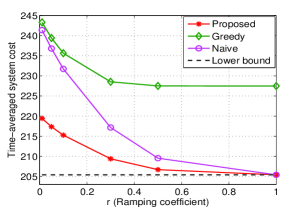
Figure 6: System cost vs. ramping coefficient $r$ (large loads).

Figure 7: Performance gap vs. number of iterations for distributed algorithm.

In Fig. 7, we exhibit the convergence of the proposed distributed algorithm for a particular system realization. The value of the penalty parameter $\rho$ needs to be adjusted for good convergence performance and is set to $5$ in our case. For comparison, we also show the convergence of a subgradient algorithm [31]. The vertical axis denotes the gap between the value of the objective function and the minimum value of the objective function of P5. We see that, the proposed algorithm converges fast and exhibits a linear convergence rate, while the subgradient algorithm is slow and exhibits a sublinear convergence rate. Moreover, the fast convergence of the proposed algorithm is observed in general, and we omit the curves of the other system realizations for brevity.

VI Conclusion and Future Work

We have investigated the problem of power balancing in a renewable-integrated power grid with storage and flexible loads. With the objective of minimizing the system cost, we have proposed a distributed real-time algorithm, which is fast converging and is asymptotically optimal as the storage capacity increases and the ramping constraint of the CG becomes loose.

There are several possible directions for the future work. For example, first, in the proposed real-time algorithm, only the current observations of the system states are employed in the algorithm design. In reality, forecasts of the system states (e.g., wind generation, loads, and electricity prices) are usually available within a certain time interval. Therefore, it would be interesting to study how to incorporate these forecasts into the algorithm design and how these forecasts could improve the algorithm performance. Second, the specific implementation of curtailing the flexible loads is not considered in this paper. How to incentivize individual customers to participate in such power balancing service and other demand response programs is currently open and worth further investigation.

Appendix A Proof of Relaxation from P1 to P2

Using the energy state update in (4) we can derive that the left hand side of constraint (11) equals the following:

$$\lim_{T\to\infty}\;\frac{1}{T}\sum_{t=0}^{T-1}\mathbb{E}[x_{i,t}]=\lim_{T\to\infty}\;\frac{\mathbb{E}[s_{i,T}]}{T}-\lim_{T\to\infty}\;\frac{\mathbb{E}[s_{i,0}]}{T}.$$ (22)

In (22), if $s_{i,t}$ is always bounded, i.e., constraint (5) holds, then the right hand side of (22) equals zero and thus constraint (11) is satisfied. Therefore, P2 is a relaxed problem of P1.

Appendix B Upper bound on drift-plus-cost function

In the following lemma, we show that the drift-plus-cost function is upper bounded.

Lemma 1

For all possible decisions and all possible values of $\mathbf{\Theta}_{t}$, in each time slot $t$, the drift-plus-cost function is upper bounded as follows:

$$\Delta(\mathbf{\Theta}_{t})+V\mathbb{E}[w_{t}|\mathbf{\Theta}_{t}]\leq B+J_{t}\mathbb{E}\left[\frac{l_{b,t}+l_{f,t}-l_{m,t}}{l_{f,t}}-\alpha\Big{|}\mathbf{\Theta}_{t}\right]$$

$$\hskip 28.45274pt+\sum_{i=1}^{N}(s_{i,t}-\beta_{i})\mathbb{E}\big{[}x_{i,t}|\mathbf{\Theta}_{t}\big{]}+V\mathbb{E}[w_{t}|\mathbf{\Theta}_{t}]$$ (23)

where $B$ is a constant and is given by $B{\triangleq}\frac{1}{2}(1+\alpha^{2})+\frac{1}{2}\sum_{i=1}^{N}\max\{x_{i,\min}^{2},x_{i,\max}^{2}\}.$

Proof:

Based on the definition of $L(\mathbf{\Theta}_{t})$, the difference

$$L(\mathbf{\Theta}_{t+1})-L(\mathbf{\Theta}_{t})$$

$$=\frac{1}{2}\left[\sum_{i=1}^{N}(s_{i,t+1}-\beta_{i})^{2}-(s_{i,t}-\beta_{i})^{2}\right]+\frac{1}{2}(J_{t+1}^{2}-J_{t}^{2}).$$ (24)

From the iteration of $J_{t}$ in (12), $(J_{t+1}^{2}-J_{t}^{2})$ in (B) can be upper bounded as

$$J_{t+1}^{2}-J_{t}^{2}\leq 2J_{t}\left(\frac{l_{b,t}+l_{f,t}-l_{m,t}}{l_{f,t}}-\alpha\right)+1+\alpha^{2}.$$ (25)

From the iteration of $s_{i,t}$ in (4), $[(s_{i,t+1}-\beta_{i})^{2}-(s_{i,t}-\beta_{i})^{2}]$ in (B) can be upper bounded as

$$(s_{i,t+1}-\beta_{i})^{2}-(s_{i,t}-\beta_{i})^{2}$$

$$\leq 2x_{i,t}(s_{i,t}-\beta_{i})+\max\{x_{i,\min}^{2},x_{i,\max}^{2}\}.$$ (26)

Applying inequalities (25) and (26) to (B), taking the conditional expectation given $\mathbf{\Theta}_{t}$, and adding the term $V\mathbb{E}[w_{t}|\mathbf{\Theta}_{t}]$ yields the upper bound in (23). ∎

Appendix C Proof of Proposition 1

To prove the feasibility under Algorithm 1, we are left to show that the long-term constraint (2) and the energy state constraint (5) are satisfied.

For constraint (2), under the Lyapunov optimization framework, it suffices to show that the virtual queue $J_{t}$ is mean rate stable, i.e., $\lim_{T\to\infty}\frac{\mathbb{E}[J_{i,T}]}{T}=0$ (see Section 4.4 in [17]). Using Proposition 3.1 that $J_{t}$ is upper bounded we can easily prove this identity.

To prove that constraint (5) is satisfied, we first show the following lemma which gives a sufficient condition for charging or discharging.

Lemma 2

1. If $s_{i,t}<-x_{i,\min}+s_{i,\min}$, then $x_{i,t}^{*}=\min\{a_{i,t},x_{i,\max}\}$.

2. If $s_{i,t}>\beta_{i}-V(p_{s,\min}+D^{\prime}_{i,\min})$, then $x_{i,t}^{*}=x_{i,\min}$.

Proof:

To show Lemma 2.1), we first transform P3 to an equivalent problem P3a) by eliminating the variables $e_{b,t}$ and $b_{i,t},\forall i$, and the constant terms.

$$\textbf{P3a)}:\min\; \textstyle{\big{[}\sum_{i=1}^{N}VD_{i}(x_{i,t})+(s_{i,t}-\beta_{i})x_{i,t}\big{]}+VC(g_{t})}$$

$$\textstyle{+Vp_{b,t}\big{(}e_{s,t}+l_{m,t}-g_{t}+\sum_{i=1}^{N}x_{i,t}\big{)}-Vp_{s,t}e_{s,t}-\frac{J_{t}}{l_{f,t}}l_{m,t}}$$

s.t. $$\eqref{conl},\eqref{cong},\eqref{congr},e_{s,t}\geq 0$$

$$x_{i,\min}\leq x_{i,t}\leq\min\{a_{i,t},x_{i,\max}\}$$ (27)

$$\textstyle{x_{i,t}\geq\sum_{i=1}^{N}a_{i,t}-\sum_{j\neq i}^{N}x_{j,t}-l_{m,t}+g_{t}-e_{s,t}}.$$ (28)

We solve P3a) by the partitioning method. Specifically, we first fix the variables $\big{(}(x_{j,t})_{j\neq i},l_{m,t},g_{t},e_{s,t}\big{)}$ and minimize P3a) over $x_{i,t}$. Since the objective function of P3a) is separable over all variables, an optimal solution of $x_{i,t}$ can be derived by the following problem:

$$\min_{x_{i,t}}\quad VD_{i}(x_{i,t})+(s_{i,t}-\beta_{i})x_{i,t}+Vp_{b,t}x_{i,t}$$

s.t. $$\eqref{xrg},\eqref{xge}.$$

Under the assumption that $s_{i,t}<\beta_{i}-V(p_{b,\max}+D^{\prime}_{i,\max})=-x_{i,\min}+s_{i,\min}$, the objective function above is strictly decreasing with respect to $x_{i,t}$. Therefore, the optimal solution of $x_{i,t}$ is $\min\{a_{i,t},x_{i,\max}\}$.

The demonstration of Lemma 2.2 is similar to that of Lemma 2.1. We first transform P3 to an equivalent problem P3b) by eliminating the variables $e_{s,t}$ and $b_{i,t},\forall i$, and the constant terms. To solve the problem, we first fix the variables $\big{(}(x_{j,t})_{j\neq i},l_{m,t},g_{t},e_{b,t}\big{)}$ and minimize P3b) over $x_{i,t}$. By some arrangement, an optimal solution of $x_{i,t}$ can be derived by the following problem:

$$\min_{x_{i,t}}\quad VD_{i}(x_{i,t})+(s_{i,t}-\beta_{i})x_{i,t}+Vp_{s,t}x_{i,t}$$

s.t. $$\eqref{xrg}$$

$$\textstyle{x_{i,t}\leq\sum_{i=1}^{N}a_{i,t}-\sum_{j\neq i}^{N}x_{j,t}-l_{m,t}+g_{t}+e_{b,t}}.$$

When $s_{i,t}>\beta_{i}-V(p_{s,\min}+D^{\prime}_{i,\min})$, the objective function above is strictly increasing with respect to $x_{i,t}$. Therefore, the optimal solution of $x_{i,t}$ is $x_{i,\min}$. ∎

Using Lemma 2, we can show that constraint (5) holds by mathematical induction.

Lemma 3

For the $i$-th storage unit, the energy state $s_{i,t}$ is bounded within the interval $[s_{i,\min},s_{i,\max}]$.

Proof:

The basis: For $t=0$, we have $s_{i,0}\in[s_{i,\min},s_{i,\max}]$ for the initial setup.

The inductive step: Assume that $s_{i,t}\in[s_{i,\min},s_{i,\max}]$. Then we need to show that $s_{i,t+1}\in[s_{i,\min},s_{i,\max}]$. In the following, we discuss three cases of $s_{i,t}$.

1. $s_{i,t}\in[s_{i,\min},-x_{i,\min}+s_{i,\min})$. Using Lemma 2.1) and the iteration of $s_{i,t}$ in (4), we have $s_{i,t+1}=s_{i,t}+\min\{a_{i,t},x_{i,\max}\}\geq s_{i,t}\geq s_{i,\min}$. Also, we have $s_{i,t+1}\leq s_{i,t}+x_{i,\max}<s_{i,\max}$ where the last inequality is derived based on the assumption of $s_{i,t}$ and $V_{\max}>0$.

2. $s_{i,t}\in[-x_{i,\min}+s_{i,\min},\beta_{i}-V(p_{s,\min}+D^{\prime}_{i,\min})]$. Based on the iteration in (4), we have $s_{i,t+1}\in[s_{i,t}+x_{i,\min},s_{i,t}+x_{i,\max}]$. By the definitions of $\beta_{i}$ and $V_{\max}$ we can derive that $s_{i,t+1}\in[s_{i,\min},s_{i,\max}]$.

3. $s_{i,t}\in(\beta_{i}-V(p_{s,\min}+D^{\prime}_{i,\min}),s_{i,\max}]$. Using Lemma 2.2) and the iterations in (4), we have $s_{i,t+1}=s_{i,t}+x_{i,\min}<s_{i,t}\leq s_{i,\max}$. Also, we have $s_{i,t+1}>s_{i,\min}$ according to the assumption of $s_{i,t}$ and the definition of $\beta_{i}$.

∎

Appendix D Proof of Theorem 1

1) Note that P2 fits the standard Lyapunov optimization format (see Section 4.3 in [17] for details of the standard format). The idea of showing performance of Algorithm 1 is to connect Algorithm 1 with the algorithm for P2 that is designed under the Lyapunov optimization framework. Before showing performance of Algorithm 1, we give two lemmas, which will be used later.

In the following lemma, we show the existence of a special algorithm for P2. Denote $\tilde{w}$ as the optimal system cost of P2.

Lemma 4

For P2, there exists a stationary and randomized solution $\mathbf{u}_{t}^{s}$ that only depends on the system states $\mathbf{q}_{t}$, and at the same time satisfies the following conditions:

$$\mathbb{E}[w_{t}^{s}]\leq\tilde{w},\quad\forall t,$$ (29)

$$\mathbb{E}[x_{i,t}^{s}]=0,\quad\forall i,t,$$ (30)

$$\mathbb{E}\left[\frac{l_{b,t}+l_{f,t}-l_{m,t}^{s}}{l_{f,t}}\right]\leq\alpha,\quad\forall t$$ (31)

where all expectations are taken over the randomness of the system state and the possible randomness of the decisions.

Proof:

The claims above can be derived from Theorem 4.5 in [17]. In particular, that theorem provides sufficient conditions for the existence of a stationary and randomized algorithm as described above. It can be checked that these sufficient conditions are all met in our problem. Therefore, the conclusion in Lemma 4 holds. ∎

By minimizing the upper bound of the drift-plus-cost function (i.e., the right hand side of (23)), the real-time sub-problem for P2 at time slot $t$ is given by

$$\textbf{P3'}:\;\min_{\mathbf{u}_{t}}\quad \left[\sum_{i=1}^{N}VD_{i}(x_{i,t})+(s_{i,t}-\beta_{i})x_{i,t}\right]+VC(g_{t})$$

$$+Vp_{b,t}e_{b,t}-Vp_{s,t}e_{s,t}-\frac{J_{t}}{l_{f,t}}l_{m,t}$$

s.t. $$\eqref{conl},\eqref{conx},\eqref{conb}-\eqref{cong},\eqref{cone},\eqref{conmbl}.$$

Note that P3’ is the same as P3 except without the ramping constraint (8). Denote the optimal objective values of P3’ and P3 as $\tilde{f}_{t}$ and $f_{t}^{*}$, respectively, and denote an optimal solution of P3’ and P3 as $\tilde{\mathbf{u}}_{t}$ and $\mathbf{u}_{t}^{*}$, respectively. In the following lemma, we characterize $f_{t}^{*}$ in terms of $\tilde{f}_{t}$.

Lemma 5

At each time slot, $f_{t}^{*}$ is bounded as $\tilde{f}_{t}\leq f_{t}^{*}\leq\tilde{f}_{t}+\epsilon$, where

$$\epsilon{\triangleq}V(1-r)g_{\max}\max\{p_{b,\max},C^{\prime}_{\max}\}.$$

Proof:

First, since P3 has more restricted constraints than P3’, there is $f_{t}^{*}\geq\tilde{f}_{t}$.

Next, we are to upper bound $f_{t}^{*}-\tilde{f}_{t}$. Comparing the solution $g_{t}^{*}$ of P3 with the solution $\tilde{g}_{t}$ of P3’ there are three possibilities:

1. $g_{t}^{*}=\tilde{g}_{t}$,

2. $g_{t}^{*}<\tilde{g}_{t}$ (less output due to constraint (8)), and

3. $g_{t}^{*}>\tilde{g}_{t}$ (more output due to constraint (8)).

For Case 1), it is easy to show that $f_{t}^{*}=\tilde{f}_{t}$. Thus, we focus on the latter two cases.

Denote a feasible solution of P3 as $\hat{\mathbf{u}}_{t}$ and its corresponding objective value as $\hat{f}_{t}$. Since characterizing the gap $f_{t}^{*}-\tilde{f}_{t}$ directly is challenging, we instead consider the gap $\hat{f}_{t}-\tilde{f}_{t}$.

For Case 2), when $g_{t}^{*}<\tilde{g}_{t}$, the effective constraint of $g_{t}$ in P3 should be $\max\{g_{t-1}-rg_{\max},0\}\leq g_{t}\leq g_{t-1}+rg_{\max}$. Set a feasible solution of P3 as $\hat{\mathbf{u}}_{t}=[\tilde{\mathbf{b}}_{t},\tilde{\mathbf{x}}_{t},\tilde{l}_{m,t},g_{t-1}+rg_{\max},\tilde{e}_{b,t}+\tilde{g}_{t}-g_{t-1}-rg_{\max},\tilde{e}_{s,t}].$ That is, $\hat{\mathbf{u}}_{t}$ is the same as $\tilde{\mathbf{u}}_{t}$ except the solutions of $g_{t}$ and $e_{b,t}$. Intuitively, we can interpret $\hat{\mathbf{u}}_{t}$ as that, due to the ramping constraint, the CG is forced to generate less energy, and the aggregator chooses to buy more from the external energy markets to balance power. The gap $\hat{f}_{t}-\tilde{f}_{t}$ is given by

$$\hat{f}_{t}-\tilde{f}_{t}$$

$$=V\big{[}C(g_{t-1}+rg_{\max})-C(\tilde{g}_{t})+p_{b,t}(\tilde{g}_{t}-g_{t-1}-rg_{\max})\big{]}$$

$$\leq Vp_{b,t}(\tilde{g}_{t}-g_{t-1}-rg_{\max})$$ (32)

$$\leq V(1-r)g_{\max}p_{b,\max}$$ (33)

where the inequality in (32) holds since $\tilde{g}_{t}>g_{t-1}+rg_{\max}$ and the function $C(\cdot)$ is non-decreasing. From (33), the gap $f_{t}^{*}-\tilde{f}_{t}$ is upper bounded by

$$f_{t}^{*}-\tilde{f}_{t}\leq\hat{f}_{t}-\tilde{f}_{t}\leq V(1-r)g_{\max}p_{b,\max}.$$ (34)

The proof for Case 3) is similar as that for Case 2). In particular, when $g_{t}^{*}>\tilde{g}_{t}$, the effective constraint of $g_{t}$ in P3 should be $g_{t-1}-rg_{\max}\leq g_{t}\leq\min\{g_{\max},g_{t-1}+rg_{\max}\}$. Set a feasible solution of P3 as $\hat{\mathbf{u}}_{t}=[\tilde{\mathbf{b}}_{t},\tilde{\mathbf{x}}_{t},\tilde{l}_{m,t},g_{t-1}-rg_{\max},\tilde{e}_{b,t},\tilde{e}_{s,t}-\tilde{g}_{t}+g_{t-1}-rg_{\max}].$ That is, $\hat{\mathbf{u}}_{t}$ is the same as $\tilde{\mathbf{u}}_{t}$ except the solutions of $g_{t}$ and $e_{s,t}$. Intuitively, we can interpret $\hat{\mathbf{u}}_{t}$ as that, due to the ramping constraint, the CG is forced to generate more energy, and the aggregator chooses to sell more to the external energy markets to balance power. The gap $\hat{f}_{t}-\tilde{f}_{t}$ is given by

$$\hat{f}_{t}-\tilde{f}_{t}$$

$$=V\big{[}C(g_{t-1}-rg_{\max})-C(\tilde{g}_{t})+p_{s,t}(\tilde{g}_{t}-g_{t-1}+rg_{\max})\big{]}$$

$$\leq V\big{[}C(g_{t-1}-rg_{\max})-C(\tilde{g}_{t})\big{]}$$ (35)

$$\leq V(g_{t-1}-rg_{\max}-\tilde{g}_{t})C^{\prime}_{\max}$$ (36)

$$\leq V(1-r)g_{\max}C^{\prime}_{\max}$$ (37)

where the inequality in (35) holds since $\tilde{g}_{t}<g_{t-1}-rg_{\max}$, and the inequality (36) is derived by the mean value theorem. From (37), we have

$$f_{t}^{*}-\tilde{f}_{t}\leq\hat{f}_{t}-\tilde{f}_{t}\leq V(1-r)g_{\max}C^{\prime}_{\max}.$$ (38)

Combining (34) and (38) yields $f_{t}^{*}\leq\tilde{f}_{t}+V(1-r)g_{\max}\max\{p_{b,\max},C^{\prime}_{\max}\}$, which completes the proof. ∎

Using Lemmas 1, 4, and 5, the drift-plus-cost function under Algorithm 1 can be upper bounded below:

$$\Delta(\mathbf{\Theta}_{t})+V\mathbb{E}[{w}_{t}^{*}|\mathbf{\Theta}_{t}]$$

$$\leq B+\epsilon+J_{t}\mathbb{E}\left[\frac{l_{b,t}+l_{f,t}-\tilde{l}_{m,t}}{l_{f,t}}-\alpha\Big{|}\mathbf{\Theta}_{t}\right]$$

$$\hskip 28.45274pt+\sum_{i=1}^{N}(s_{i,t}-\beta_{i})\mathbb{E}\big{[}\tilde{x}_{i,t}|\mathbf{\Theta}_{t}\big{]}+V\mathbb{E}[\tilde{w}_{t}|\mathbf{\Theta}_{t}]$$ (39)

$$\leq B+\epsilon+J_{t}\mathbb{E}\left[\frac{l_{b,t}+l_{f,t}-l_{m,t}^{s}}{l_{f,t}}-\alpha\Big{|}\mathbf{\Theta}_{t}\right]$$

$$\hskip 28.45274pt+\sum_{i=1}^{N}(s_{i,t}-\beta_{i})\mathbb{E}\big{[}x_{i,t}^{s}|\mathbf{\Theta}_{t}\big{]}+V\mathbb{E}[w_{t}^{s}|\mathbf{\Theta}_{t}]$$ (40)

$$\leq B+\epsilon+V\tilde{w}$$ (41)

$$\leq B+\epsilon+Vw^{\textrm{opt}}$$ (42)

where (39) is derived by Lemmas 1 and 5, (40) holds since P3’ minimizes the right hand side of (39), (41) is derived based on (29)(30)(31) in Lemma 4 and the fact that $\mathbf{u}_{t}^{s}$ is independent of $\mathbf{\Theta}_{t}$, and (42) holds since P2 is a relaxed problem of P1.

Taking expectations over $\mathbf{\Theta}_{t}$ on both sides of (42) and summing over $t\in\{0,\cdots,T-1\}$ yields

$$\mathbb{E}[L(\mathbf{\Theta}_{T})]-\mathbb{E}[L(\mathbf{\Theta}_{0})]+V\sum_{t=0}^{T-1}\mathbb{E}[{w}_{t}^{*}]\leq(B+\epsilon+Vw^{\textrm{opt}})T.$$ (43)

Since $L(\mathbf{\Theta}_{T})$ is non-negative, after some arrangement, from (43) there is

$$\frac{1}{T}\sum_{t=0}^{T-1}\mathbb{E}[{w}_{t}^{*}]\leq\frac{B+\epsilon+Vw^{\textrm{opt}}}{V}+\frac{\mathbb{E}[L(\mathbf{\Theta}_{0})]}{TV}.$$ (44)

Taking $\limsup$ on both sides of (44) and rearranging the terms gives $w^{*}-w^{\textrm{opt}}\leq B/V+(1-r)g_{\max}\max\{p_{b,\max},C^{\prime}_{\max}\}.$ To emphasize the dependence of performance on $r$ and $V$, we express $w^{*}$ as $w^{*}(r,V)$. Similarly, we express $w^{\textrm{opt}}$ as $w^{\textrm{opt}}(r)$.

2) The lower bound on $w^{\textrm{opt}}(r)$ can be derived by setting $r=1$ in Theorem 1.1 and recognizing that $w^{\textrm{opt}}(1)\leq w^{\textrm{opt}}(r)$.

Appendix E Proof of Proposition 2

Proposition 2 can be shown by mathematical induction. The proof resembles that of Lemma 3 where the energy capacity $s_{i,\max}$ is replaced by $s_{i,\textrm{up}}$. We omit the proof for brevity.

Appendix F Proof of Proposition 3

1) We prove the conclusion by mathematical induction.

The basis: For $t=0$, we have $J_{t}=0$, which is obviously upper bounded.

The inductive step: Assume that $J_{t}\leq Vp_{b,\max}l_{f,\max}+1$. Then we need to show that $J_{t+1}\leq Vp_{b,\max}l_{f,\max}+1$. Consider the following two cases of $J_{t}$.

1. $J_{t}\leq Vp_{b,\max}l_{f,\max}$. Based on the update of $J_{t}$ in (12), we have $J_{t+1}\leq\max\{J_{t}-\alpha,0\}+1\leq J_{t}+1\leq Vp_{b,\max}l_{f,\max}+1$.

2. $J_{t}\in(Vp_{b,\max}l_{f,\max},Vp_{b,\max}l_{f,\max}+1]$. For this case, we will show that the unique solution of $l_{m,t}$ to P3 is $l_{b,t}+l_{f,t}$. Hence, $J_{t+1}=\max\{J_{t}-\alpha,0\}\leq J_{t}\leq Vp_{b,\max}l_{f,\max}+1$.

   To this end, we consider the equivalent problem P3a). First fix the variables $\big{(}\mathbf{x}_{t},g_{t},e_{s,t}\big{)}$ and minimize P3a) over $l_{m,t}$. After some arrangement, an optimal solution of $l_{m,t}$ can be derived by the following problem:

   $$\min_{l_{m,t}}\quad \big{(}Vp_{b,t}-\frac{J_{t}}{l_{f,t}}\big{)}l_{m,t}$$

   s.t. $$l_{b,t}\leq l_{m,t}\leq l_{b,t}+l_{f,t},$$

   $$l_{m,t}\geq\sum_{i=1}^{N}(a_{i,t}-x_{i,t})+g_{t}-e_{s,t}.$$

   When $J_{t}>Vp_{b,\max}l_{f,\max}$, the objective function above is strictly decreasing. Therefore, the optimal solution of $l_{m,t}$ is $l_{b,t}+l_{f,t}$.

2) We prove the conclusion by contradiction. Suppose that under our algorithm the optimal solutions of $e_{b,t}$ and $e_{s,t}$ satisfy $e_{b,t}^{*}>e_{s,t}^{*}>0$. Then, we can show that there is another feasible solution $\hat{\mathbf{u}}_{t}=\left[\mathbf{b}_{t}^{*},\mathbf{x}_{t}^{*},l_{m,t}^{*},g_{t}^{*},e_{b,t}^{*}-e_{s,t}^{*},0\right]$ achieving a strictly smaller objective value, hence contradicting the fact that $\mathbf{u}_{t}^{*}$ is optimal. The proofs of the other two possible cases, i.e., $e_{b,t}^{*}=e_{s,t}^{*}>0$ and $e_{s,t}^{*}>e_{b,t}^{*}>0$, are similar, and are omitted for brevity.

Appendix G Simplification of (17)-(19)

Define $\overline{y}^{k}{\triangleq}\frac{1}{N+4}\sum_{i=1}^{N+4}y_{i}^{k}$ and $\overline{d}^{k}{\triangleq}\frac{1}{N+4}\sum_{i=1}^{N+4}d_{i}^{k}$ as the averages of $y_{i}^{k}$ and $d_{i}^{k}$ over $i$ at the $k$-th iteration, respectively. By solving the minimization problem in (18), we can get a closed-form solution of $z_{i}^{k+1}$ below:

$$z_{i}^{k+1}=\frac{d_{i}^{k}}{\rho}+y_{i}^{k+1}-\frac{\overline{d}^{k}}{\rho}-\overline{y}^{k+1}+\frac{\sum_{i=1}^{N}a_{i}}{N+4}.$$ (45)

Substituting the right hand side of (45) for $z_{i}^{k+1}$ in the $\mathbf{d}$-update (19) yields $d_{i}^{k+1}=\overline{d}^{k}+\rho(\overline{y}^{k+1}-\frac{\sum_{i=1}^{N}a_{i}}{N+4})$, which indicates that the dual variables $d_{i}^{k+1}$ are identical for all $i$ at each iteration. Therefore, we can safely drop the subscript $i$ in $d_{i}^{k+1}$ and obtain the $d$-update in (21). Meanwhile, substituting the right hand side of (45) for $z_{i}^{k}$ in the $\mathbf{y}$-update (17) and using the fact that $d_{i}^{k-1}$ are identical for all $i$ yields (20). Since the vector $\mathbf{z}$ is not employed in either $\mathbf{y}$-update or $d$-update, it can be eliminated.

Sun Sun (S’11) received the B.S. degree in Electrical Engineering and Automation from Tongji University, Shanghai, China, in 2005. From 2006 to 2008, she was a software engineer in the Department of GSM Base Transceiver Station of Huawei Technologies Co. Ltd.. She received the M.Sc. degree in Electrical and Computer Engineering from University of Alberta, Edmonton, Canada, in 2011. Now, she is pursuing her Ph.D. degree in the Department of Electrical and Computer Engineering of University of Toronto, Toronto, Canada. Her current research interest lies in the areas of stochastic optimization, distributed control, learning, and economics, with the application of renewable generation, energy storage, demand response, and power system operations.

Min Dong (S’00-M’05-SM’09) received the B.Eng. degree from Tsinghua University, Beijing, China, in 1998, and the Ph.D. degree in electrical and computer engineering with minor in applied mathematics from Cornell University, Ithaca, NY, in 2004. From 2004 to 2008, she was with Corporate Research and Development, Qualcomm Inc., San Diego, CA. In 2008, she joined the Department of Electrical, Computer and Software Engineering at University of Ontario Institute of Technology, Ontario, Canada, where she is currently an Associate Professor. She also holds a status-only Associate Professor appointment with the Department of Electrical and Computer Engineering, University of Toronto since 2009. Her research interests are in the areas of statistical signal processing for communication networks, cooperative communications and networking techniques, and stochastic network optimization in dynamic networks and systems. She served as an Associate Editor for the IEEE TRANSACTIONS ON SIGNAL PROCESSING (2010–2014), and as an Associate Editor for the IEEE SIGNAL PROCESSING LETTERS (2009–2013). She was a technical lead co-chair of the Communications and Networks to Enable the Smart Grid Symposium at the IEEE International Conference on Smart Grid Communications (SmartGridComm) in 2014. She has been an elected member of the IEEE Signal Processing Society Signal Processing for Communications and Networking (SP-COM) technical committee since 2013. She was the recipient of the Early Researcher Award from Ontario Ministry of Research and Innovation in 2012, the Best Paper Award at IEEE ICCC in 2012, and the 2004 IEEE Signal Processing Society Best Paper Award.

Ben Liang (S’94-M’01-SM’06) received honors-simultaneous B.Sc. (valedictorian) and M.Sc. degrees in Electrical Engineering from Polytechnic University in Brooklyn, New York, in 1997 and the Ph.D. degree in Electrical Engineering with Computer Science minor from Cornell University in Ithaca, New York, in 2001. In the 2001 - 2002 academic year, he was a visiting lecturer and post-doctoral research associate at Cornell University. He joined the Department of Electrical and Computer Engineering at the University of Toronto in 2002, where he is now a Professor. His current research interests are in mobile communications and networked systems. He has served as an editor for the IEEE Transactions on Wireless Communications and an associate editor for the Wiley Security and Communication Networks journal, in addition to regularly serving on the organizational or technical committee of a number of conferences. He is a senior member of IEEE and a member of ACM and Tau Beta Pi.

References

- [1] A. Meier, Electric Power Systems: A Conceptual Introduction. Wiley-IEEE Press, 2006.
- [2] P. Denholm, E. Ela, B. Kirby, and M. Milligan, “The role of energy storage with renewable electricity generation,” National Renewable Energy Laboratory, Tech. Rep., Jan. 2010.
- [3] D. Callaway and I. Hiskens, “Achieving controllability of electric loads,” Proc. IEEE, vol. 99, no. 1, pp. 184–199, Jan. 2011.
- [4] H. Su and A. Gamal, “Modeling and analysis of the role of energy storage for renewable integration: Power balancing,” IEEE Trans. Power Syst., vol. 28, no. 4, pp. 4109–4117, Nov. 2013.
- [5] L. Lu, J. Tu, C. Chau, M. Chen, and X. Lin, “Online energy generation scheduling for microgrids with intermittent energy sources and co-generation,” in Proc. ACM Sigmetrics, Jun. 2013.
- [6] B. Narayanaswamy, V. Garg and T. Jayram, “Online optimization for the smart (micro) grid,” in ACM e-Energy, May 2012.
- [7] T. Chang, M. Alizadeh, and A. Scaglione, “Real-time power balancing via decentralized coordinated home energy scheduling,” IEEE Trans. Smart Grid, vol. 4, no. 3, pp. 1490–1504, Sep. 2013.
- [8] S. Sun, M. Dong, and B. Liang, “Real-time power balancing in electric grids with distributed storage,” IEEE J. Sel. Topics Signal Process., vol. 8, no. 6, pp. 1167–1181, Dec. 2014.
- [9] ——, “Real-time welfare-maximizing regulation allocation in dynamic aggregator-EVs system,” IEEE Trans. Smart Grid, vol. 5, no. 3, pp. 1397–1409, May 2014.
- [10] L. Huang, J. Walrand, and K. Ramchandran, “Optimal power procurement and demand response with quality-of-usage guarantees,” in Proc. IEEE PESGM, Jul. 2012.
- [11] L. Xiang, D. Ng, W. Lee, and R. Schober, “Optimal storage-aided wind generation integration considering ramping requirements,” in Proc. IEEE SmartGridComm., Oct. 2013.
- [12] Y. Huang, S. Mao, and R. Nelms, “Adaptive electricity scheduling in microgrids,” in Proc. IEEE INFOCOM, Apr. 2013.
- [13] S. Chen, N. Shroff, and P. Sinha, “Heterogeneous delay tolerant task scheduling and energy management in the smart grid with renewable energy,” IEEE J. Sel. Areas Commun., vol. 31, no. 7, pp. 1258–1267, Jul. 2013.
- [14] Y. Guo, M. Pan, Y. Fang, and P. Khargonekar, “Decentralized coordination of energy utilization for residential households in the smart grid,” IEEE Trans. Smart Grid, vol. 4, no. 3, pp. 1341–1350, Sep. 2013.
- [15] Y. Zhang, N. Gatsis, and G. Giannakis, “Robust energy management for microgrids with high-penetration renewables,” IEEE Trans. Sustainable Enery, vol. 4, no. 4, pp. 944–953, Oct. 2013.
- [16] S. Salinas, M. Li, P. Li, and Y. Fu, “Dynamic energy management for the smart grid with distributed energy resources,” IEEE Trans. Smart Grid, vol. 4, no. 4, pp. 2139–2150, Dec. 2013.
- [17] M. Neely, Stochastic Network Optimization with Application to Communication and Queueing Systems. Morgan & Claypool, 2010.
- [18] S. Boyd, N. Parikh, E. Chu, B. Peleato, and J. Eckstein, Distributed Optimization and Statistical Learning via the Alternating Direction Method of Multipliers. Found. Trends Mach. Learning, 2011.
- [19] J. Qin, Y. Chow, J. Yang, and R. Rajagopal, “Distributed online modified greedy algorithm for networked storage operation under uncertainty,” Jun. 2014. [Online]. Available: http://arxiv.org/pdf/1406.4615v2.pdf
- [20] Y. Kanoria, A. Montanari, D. Tse, and B. Zhang, “Distributed storage for intermittent energy sources: Control design and performance limits.” [Online]. Available: http://arxiv.org/abs/1110.4441
- [21] J. Kim and W. Powell, “Optimal energy commitments with storage and intermittent supply,” Oper. Res., vol. 59, no. 6, p. 1347–1360, Nov.-Dec. 2011.
- [22] A. ParandehGheibi, M. Roozbehani, A. Ozdaglar, and M. Dahleh, “The reliability value of storage in a volatile environment,” in Proc. ACC, Jun. 2012.
- [23] S. Bose and E. Bitar, “Variability and the locational marginal value of energy storage,” in Proc. IEEE CDC, Dec. 2014.
- [24] S. Sun, M. Dong, and B. Liang, “Joint supply, demand, and energy storage management towards microgrid cost minimization,” in Proc. IEEE SmartGridComm, Nov. 2014.
- [25] P. Ramadass, B. Haran, R. White, and B. Popov, “Performance study of commercial LiCoO2 and spinel-based Li-ion cells,” J. Power Sources, vol. 111, no. 2, pp. 210–220, Apr. 2002.
- [26] M. Shahidehpour, H. Yamin, and Z. Li, Market Operations in Electric Power Systems: Forecasting, Scheduling, and Risk Management. Wiley-IEEE Press, 2002.
- [27] S. Nadel and G. Herndon, The Future of the Utility Industry and the Role of Energy Efficiency. Washington, DC, 2014.
- [28] H. Wang and A. Banerjee, “Online alternating direction method.” [Online]. Available: http://arxiv.org/abs/1306.3721
- [29] A. Ipakchi and F. Albuyeh, “Grid of the future,” IEEE Power Energy Mag., vol. 7, no. 2, pp. 52–62, 2009.
- [30] “Electricity prices in Ontario.” [Online]. Available: http://www.ontarioenergyboard.ca/OEB/Consumers/Electricity
- [31] T. Larsson, M. Patriksson, and A. Strömberg, “Ergodic, primal convergence in dual subgradient schemes for convex programming,” Math. Program., vol. 86, pp. 283–312, 1999.